Asymmetric inflation: exact solutions

Abstract

We provide exact solutions to the Einstein equations when the Universe contains vacuum energy plus a uniform arrangements of magnetic fields, strings, or domain walls. Such a universe has planar symmetry, i. e., it is homogeneous but, not isotropic. Further exact solutions are obtained when dust is included and approximate solutions are found for $w\not=0$ matter. These cosmologies also have planar symmetry. These results may eventually be used to explain some features in the WMAP data. The magnetic field case is the easiest to motivate and has the highest possibility of yielding reliable constraints on observational cosmology.

today

I Introduction

After many successes, standard radiation/matter dominated Big Bang cosmology was found inadequate to provide solutions to a number of problems raised when the model was studied in more detail in the light of modern data. These problems include the horizon problem, the flatness problem, the magnetic monopole problem, etc. Faced with these issues, it was clear that a departure from conventional thinking was required and initial assumptions needed to be questioned. Specifically, the cosmological constant that was for many years in disfavor, was reintroduced and gave a solution to Einstein’s equations with exponentially growing scale factor, i.e., inflation Guth:1980zm ; Linde:1981mu ; Albrecht:1982wi ; Linde:1983gd . This immediately solved the problems listed above, since it allowed the universe to be in thermal equilibrium, diluted monopoles, and flattened the curvature. Inflation also allowed quantum fluctuations in the early universe to expand to super-horizon sizes. Upon re-entry the fluctuations generate the density perturbations Guth:1982ec ; Kodama:1985bj ; Mukhanov:1990me ; Liddle:1993fq that led to structure Peebles ; Padmanabhan .

As more cosmological data became available Smoot:1992td ; Bennett:1996ce ; Kogut:1996us , more detailed inflationary models have become necessary to explain it Lyth:1998xn . In the last two decades many inflationary scenarios have been analyzed Linde ; KT ; Dodelson ; KR , but all have one feature in common: homogeneous isotropic expansion. However, before the onset of inflation, a typical region of the universe is anything but homogeneous and isotropic. It is possible that an asymmetric feature in some region could be stretched out by an asymmetric inflation, but remain imprinted through the end of inflation, or that a parameter or field initially asymmetrically distributed, is diluted to a negligible value by the end of inflation, but with an imprint left on the inflated universe. Asymmetric features could also be generated by the phase transition that is responsible for the inflation. We will investigate these possibilities in models with homogeneous but anisotropic expansions.

In a previous paper Berera:2003tf we gave exact solutions of Einstein’s equations for cases of a universe with planar symmetry. These include a universe with cosmological constant plus magnetic fields, cosmic strings or cosmic domain walls aligned uniformly throughout all space. In this paper we give exact results that include non-relativistic matter (dust). We also give approximate solutions for $w\not=0$ matter.

The first year WMAP results Bennett:2003bz ; Spergel:2003cb ; Hinshaw:2003ex contain interesting large-scale features which warrant further attention Tegmark:2003ve , deOliveira-Costa:2003pu . One glaring observational feature is the suppression of power at large angular scales ($\theta\gtrsim 60^{\circ}$), which is reflected most distinctly in the reduction of the quadrupole $C_{2}$. This effect was also seen in the COBE results Smoot:1992td ; Kogut:1996us . After the COBE experiment, Monte Carlo studies were used to cast doubt on quadrupole suppression Berera:1997wz ; Berera:2000wz , suggesting the effect could just be statistical. The WMAP analysis Bennett:2003bz ; Spergel:2003cb ; Hinshaw:2003ex ; Tegmark:2003ve ; deOliveira-Costa:2003pu have arrived at similar conclusions. Nevertheless, interesting physical effects are not ruled out, especially since the octupole also appears to be somewhat suppressed. Thus it does not seem unreasonable to try to model such behavior by altering the cosmological model from the standard big bang plus inflation scenario. Intriguingly, the more precise measurements of WMAP also showed that the quadrupole $C_{2}$ and octupole $C_{3}$ are aligned. In particular, the $\ell=2$ and $3$ powers are found to be concentrated in a plane P inclined about $30^{\circ}$ to the Galactic plane. In a coordinate system in which the equator is in the plane P, the $\ell=2$ and $3$ powers are primarily in the $m=\pm\ell$ modes. The axis of this system defines a unique ray and supports the idea of power in the axial direction being suppressed relative to the power in the orthogonal plane. These effects seem to suggest one (longitudinal) direction may have expanded differently from the other two (transverse) directions, where the transverse directions describe the equatorial plane P mentioned above. Although this effect once again could be explained away as statistical Bennett:2003bz ; Spergel:2003cb ; Hinshaw:2003ex ; Tegmark:2003ve ; deOliveira-Costa:2003pu , a realistic physical model that can explain some or all anisotropic effects in the WMAP data would be of interest.

While there are many ways to approach the issue of global anisotropy of the Universe, it would be most satisfying to explain global anisotropy by a simple modification of the conventional Friedman-Robertson-Walker (FRW) model. To achieve this, one has to consider an energy-momentum tensor which is spatially non-spherical or spontaneously becomes non-spherical at each point in space-time. Such a situation could occur when defects or magnetic fields are present. Magnetic fields Kronberg:1993vk and cosmic defects Hindmarsh:1994re can arise in various ways. Moreover, it is known that large scale magnetic fields exist in the universe, perhaps up to cosmological scales Kronberg:1993vk ; Wick:2000yc . These considerations motivate us to focus our attention on the effect magnetic fields and defects can have on the expansion of the universe.

As a modest step toward understanding the form, significance and implications of an asymmetric universe, we will modify the standard spherically symmetric FRW cosmology to a form with only planar symmetry Taub:1950ez . Our choice of the energy-momentum tensor will result in non-spherical expansion  from an initially spherical symmetric configuration: an initial co-moving sphere will evolve into a spheroid that can be either prolate or oblate depending on the choice of matter content. For the sake of clarity, we first give some general properties of cosmologies with planar symmetry. (The universe looks the same from all points but the points all have a preferred axis.) Our first example will be a universe filled with dust, uniform magnetic fields and cosmological constant. (Some aspects of cosmic magnetic fields have been previously studied; see, e. g. Ref. magnetic-fields .) This is perhaps the most easily motivated, exactly solvable case to consider and it will give us a context in which to couch the discussion of other examples with planar symmetry and cases where planar symmetry is broken. We then describe a number of other exactly solvable planar symmetric cases.

To set the stage, consider an early epoch in the universe at the onset of cosmic inflation, where strong magnetic fields have been produced in a phase transition Savvidy:1977as ; Vachaspati:1991nm ; Enqvist:1994rm ; Berera:1998hv . Assuming the magnitude of the magnetic field and vacuum energy ($\Lambda$) densities are initially about the same, we will find that eventually $\Lambda$ dominates. It was estimated Vachaspati:1991nm that the initial magnetic field energy produced in the electroweak phase transition was within an order of magnitude of the critical density. Other phase transitions may have even higher initial field values Enqvist:1994rm ; Berera:1998hv , or high densities of cosmic defects. Hence, it is not unphysical to consider a universe with magnetic fields and $\Lambda$ of comparable magnitudes. If the magnetic fields are aligned in domains, then some degree of inflation is sufficient to push all but one domain outside the horizon. (Below we also discuss the cases where there is one or only a few domains within the horizon.)

Finally, we should mention that studies of departure from spherical symmetry and/or departure from standard inflationary cosmology is an active and controversial area of study. A partial list of topics includes polarization of light from astrophysical objects and related phenomena Birch:1982 ; Nodland:1997cc ; Ralston:2003pf ; Jaffe:2005pw ; Hutsemekers:2005iz , the topology of the universe Cornish:1997ab ; Luminet:2003dx ; Cornish:2003db , and low $\ell$ mode suppression Schwarz:2004gk ; Kolb:2005me . The plan of the paper follows.

In the second section we review the generalization of a FRW universe to the case of planar symmetry. We display the Christoffel symbols, Ricci tensor, and general form of the energy-momentum tensor with the corresponding Einstein equations and the general form of energy-momentum conservation. This section sets up the basic equations to be solved and also contains a discussion of thermodynamics in a planar-symmetric universe. We find a natural splitting of the elements of $T^{\mu\nu}$ into spherically symmetric and anisotropic pieces. This procedure provides key insight needed to find exact solutions for the equations of cosmic evolution. In the third section we carry out a general analysis of the features resulting from planar symmetry, and give various relations and inequalities based on energy conditions, many of which involve the eccentricity of the expansion. Various limiting cases are also considered.

Sections 4, 5 and 6 treat a universe filled with cosmological constant, dust and either uniform magnetic fields, aligned cosmic strings, or aligned cosmic domain walls, respectively. We have given each of these exactly solvable cases a separate section so that we can systematically compare and contrast them more easily. Graphics and limiting cases are both used for this purpose. The magnetic field and aligned cosmic string cases are qualitatively similar, and both are substantially different from the case of domain walls. Section 7 contains our conclusions and a brief discussion of how one would apply our results to density perturbations EccIII . An appendix has been included to treat the case of matter with generic non-zero choice for $w$, the parameter that describes the equation of state. These results are only approximate and so they have been relegated to the appendix to avoid breaking the flow of the discussion of exact results presented in the main body of the paper.

II Universe with planar symmetry

To make the simplest directionally anisotropic universe, we modify the FRW spherical symmetry of space-time into plane symmetry. (Cylindrical symmetry is, of course, not appropriate since it introduces preferred location of the axis of symmetry.) The most general form of a plane-symmetric metric (up to a conformal transformation) is Taub:1950ez

$$(g_{\mu\nu})=\textrm{diag}{(1,-\textrm{e}^{2a},-\textrm{e}^{2a},-\textrm{e}^{2b})},$$ (1)

where $a$ and $b$ are functions of $t$ and $z$; the $xy$-plane is the plane of symmetry. We also impose translational symmetry along the $z$-axis; the functions $a$ and $b$ now depend only on $t$. (Examples of plane-symmetric spaces include space uniformly filled with either uniform magnetic fields, static aligned strings, or static stacked walls, where the defects are at rest with respect to the cosmic background frame. This situation with defects is artificial or at best contrived, but could perhaps arise in brane world physics where walls could be static or walls beyond the horizon could be connected by static strings. We will not pursue these details here. Of course, any spherically-symmetric contributions (vacuum energy, matter, radiation) can be added without altering the planar symmetry.) For the metric (1), the nonzero Christoffel symbols are

$$\Gamma^{0}_{11}=\Gamma^{0}_{22}=\dot{a}\,\textrm{e}^{2a},\ \ \ \Gamma^{0}_{33}=\dot{b}\,\textrm{e}^{2b},$$

$$\Gamma^{1}_{01}=\Gamma^{2}_{02}=\dot{a},\ \ \ \Gamma^{3}_{03}=\dot{b},$$

which results in the following nonzero-components of the Ricci tensor:

$${R^{0}}_{0}=-(2\ddot{a}+\ddot{b}+2\dot{a}^{2}+\dot{b}^{2}),$$

$${R^{1}}_{1}={R^{2}}_{2}=-(\ddot{a}+2\dot{a}^{2}+\dot{a}\dot{b}),$$

$${R^{3}}_{3}=-(\ddot{b}+\dot{b}^{2}+2\dot{a}\dot{b}).$$

To support a symmetry of space-time, the energy-momentum tensor for the matter has to have the same symmetry. In the case of planar symmetry this requires

$$({T^{\mu}}_{\nu})=(8\pi G)^{-1}\textrm{diag}(\xi,\eta,\eta,\zeta).$$ (2)

Here the energy density $\xi$, transverse $\eta$ and longitudinal $\zeta$ tension densities are functions only of time. The corresponding Einstein equations are

$$\dot{a}^{2}+2\dot{a}\dot{b}=\xi,$$ (3)

$$\ddot{a}+\ddot{b}+\dot{a}^{2}+\dot{a}\dot{b}+\dot{b}^{2}=\eta,$$ (4)

$$2\ddot{a}+3\dot{a}^{2}=\zeta.$$ (5)

We also need the equation expressing covariant conservation of the energy-momentum [a direct consequence of Eqs. (3)–(5)]:

$$\dot{\xi}+2\dot{a}(\xi-\eta)+\dot{b}(\xi-\zeta)=0.$$ (6)

Table 1: The components of the energy momentum (2) for various contributions to the matter. In the text, tables and figure captions we use the labels $\Lambda$, $w$, M, S, and W to represent cosmological constant, matter with equation of state $\rho=wp$, magnetic fields, strings, and walls, respectively. Occasionally we label dust with the symbol $0$.

		$\xi$		$\eta$		$\zeta$
vacuum energy ($\Lambda$)		$\lambda$		$\lambda$		$\lambda$
matter ($w$)		$\rho$		$-w\rho$		$-w\rho$
magnetic field (M)		$\epsilon$		$-\epsilon$		$\epsilon$
strings (S)		$\epsilon$		$0$		$\epsilon$
walls (W)		$\epsilon$		$\epsilon$		$0$

We consider now the thermodynamics of cosmological models evolving anisotropically. Energy density $\rho$ and pressure $p$ correspond to the spherically-symmetric part of the energy-momentum tensor, $\xi=\lambda+\rho+\tilde{\xi}$, $\eta=\lambda-p+\tilde{\eta}$, $\zeta=\lambda-p+\tilde{\zeta}$, where we have written tildes on the anisotropic parts of the energy-momentum tensor. As in the isotropic case Weinberg , we have

$$T\textrm{d}p/\textrm{d}T=\rho+p,$$ (7)

where $T$ is the temperature. Up to an additive constant, the entropy in a volume $V$ is

$$S=(\rho+p)V/T.$$ (8)

Taking $V=V_{\textrm{i}}\,\mathrm{e}^{2a+b}$ we find

$$\dot{S}/S=2\dot{a}+\dot{b}+\dot{\rho}/(\rho+p).$$ (9)

For an adiabatic process, the entropy in a comoving volume is conserved; thus the right-hand side of Eq. (9) vanishes,

$$\dot{\rho}+(2\dot{a}+\dot{b})(\rho+p)=0.$$ (10)

For matter with the equation of state $p=w\rho$, Eq. (10) gives

$$\rho=\rho_{\textrm{i}}\,\textrm{e}^{-(1+w)(2a+b)}.$$ (11)

Eq. (10) expresses covariant conservation of the isotropic part of the energy-momentum. Since the total energy-momentum is conserved locally [Eq. (6)], the same holds for its anisotropic part,

$$\dot{\tilde{\xi}}+2\dot{a}(\tilde{\xi}-\tilde{\eta})+\dot{b}(\tilde{\xi}-\tilde{\zeta})=0.$$ (12)

Eq. (12) will be the key to finding our exact solutions.

III General properties

Before considering specific models for the energy-momentum, we first establish several general features of an anisotropic universe described by Eqs. (3)–(6). These results will be important for conceptual understanding of solutions and asymptotics bounding the effects caused by asymmetry and comparing the results for various types of asymmetric components.

• We assume that before anisotropic effects became important, the universe had expanded isotropically. During the initial phase of anisotropic expansion, when anisotropic contributions to the energy-momentum are significant, different tension densities in the longitudinal and transverse directions cause comoving spheres to evolve into spheroids. At a later phase, when all contributions except for the vacuum energy fade away, longitudinal and transverse expansion rates become equal and the expansion proceeds isotropically. Thus, in this universe, each initial sphere develops an eccentricity; whether the resulting spheroid is oblate or prolate depends on which tension dominated during the initial phase of deformation.

• We assume that initially  space is isotropic, $a_{\textrm{i}}=b_{\textrm{i}}$, and is expanding isotropically, $\dot{a}_{\textrm{i}}=\dot{b}_{\textrm{i}}>0$. Without loss of generality we set $a_{\textrm{i}}=0$, which is equivalent to a simple rescaling of scale factors $\textrm{e}^{a}$ and $\textrm{e}^{b}$. For expansion in some direction to change into contraction we need to cross the point where the expansion rate in this direction becomes zero. Since the energy density is positive, from Eq. (3) it follows that there can be no contraction in the transverse direction, $\dot{a}>0$. (See Figs. 1, 9, 17.)

• If the transverse tension is always smaller (larger) than the longitudinal tension, then initially spherical region of space-time has expanded asymptotically to the shape of an oblate (prolate) spheroid. Indeed, if $\eta<\zeta$, then Eqs. (4) and (5) give $\ddot{a}-\ddot{b}<-2\dot{a}^{2}+\dot{a}\dot{b}+\dot{b}^{2}$. Consider two cases: (i) when $\dot{a}\leq\dot{b}$, we arrive at $\ddot{a}-\ddot{b}>0$, which upon integration leads to a contradiction, $\dot{a}-\dot{b}>0$; (ii) when $\dot{a}>\dot{b}$, we find $\dot{a}-\dot{b}>2\int_{t_{\textrm{i}}}^{t}\textrm{d}t(\dot{b}^{2}-\dot{a}^{2})$, which is allowed. Similarly, if $\eta>\zeta$, then $\dot{a}\geq\dot{b}$ leads to a contradiction, while $\dot{a}<\dot{b}$ is allowed. In the allowed cases, further integration leads to the result: $a>b$ when $\eta<\zeta$, and $a<b$ when $\eta>\zeta$. (See Figs. 5, 6, 13, 14, 21, 22 for examples of different cases.)

• On the other hand, longitudinal contraction is possible. To find a moment $t=t_{*}$ when longitudinal expansion changes into contraction, we set $\dot{b}_{*}=0$ in Eqs. (3)–(5) and find $\ddot{b}_{*}=\eta_{*}+{\textstyle{\frac{1}{2}}}(\xi_{*}-\zeta_{*})$. Examining entries in Table 1 we see that, except for the case when the magnetic field dominates , $\ddot{b}_{*}$ is positive. It follows that only in the magnetic-field-dominating case, can space contract in the longitudinal direction; see Figs. 2, 10, 18 for examples of the different cases. If the initial magnetic field is sufficiently strong, the longitudinal size can become smaller then its initial value (curves with $b<0$ in Fig. 2). However, no matter how strong the initial field is, after a sufficiently long period of time contraction turns into expansion following the correct asymptotic behavior.

• For all known forms of matter the components of the energy-momentum tensor satisfy the dominant energy condition energy-momentum ; nec ; in our case it says $\xi\geq 0$, $\xi\geq\eta$, and $\xi\geq\zeta$ (see Table 1 for examples). Evaluating Eq. (6) at the initial time, we find $\dot{\xi}_{\textrm{i}}=-\dot{a}_{\textrm{i}}(3\xi_{\textrm{i}}-2\eta_{\textrm{i}}-\zeta_{\textrm{i}})$; from the energy conditions it now follows that the energy density does not increase initially, $\dot{\xi}_{\textrm{i}}\leq 0$. Let us investigate whether the energy can increase at a later time. For this to happen, we need to have $\dot{\xi}_{*}=0$ for some $t=t_{*}$; Eqs. (3) and (6) then give $\dot{a}_{*}^{2}(4\eta_{*}-3\xi_{*}-\zeta_{*})=\xi_{*}(\xi_{*}-\zeta_{*})$. This equation has a real solution for $\dot{a}_{*}$ only when the wall contribution dominates; see Table 1. However, even in the worst case, with only the wall contribution, the energy density cannot increase. Indeed, using $\xi=\eta$, we find $\dot{a}_{*}^{2}=\xi_{*}$. Since $\dot{a}>0$ by 2, Eq. (3) gives $\dot{b}_{*}=0$. In 4 we found that, unless magnetic field contribution dominates, $\ddot{b}_{*}>0$ and thus for walls $\dot{b}$ cannot become zero if initially $\dot{b}_{\textrm{i}}>0$. This proves that $\dot{\xi}\leq 0$ in all cases.

• Let us prove that the transverse expansion rate has its maximum at $t=t_{\textrm{i}}$. First, from Eqs. (3) and (5) it follows that $\ddot{a}_{\textrm{i}}={\textstyle{\frac{1}{2}}}(\zeta_{\textrm{i}}-\xi_{\textrm{i}})$ and so $\ddot{a}_{\textrm{i}}\leq 0$ because of the energy conditions in 5. It follows that $\dot{a}$ initially decreases with time. Suppose, however, that $\dot{a}$ starts increasing and reaches its initial value $\dot{a}_{\textrm{i}}$ for the first time at the moment $t_{*}$. Equation (5) then gives $\ddot{a}_{*}={\textstyle{\frac{1}{2}}}(\zeta_{*}-\xi_{\textrm{i}})$ and $\xi_{\textrm{i}}\geq\xi_{*}\geq\zeta_{*}$ from 5 leads to $\ddot{a}_{*}\leq 0$. This is impossible since to reach the first point at which $\dot{a}_{*}=\dot{a}_{\textrm{i}}$ we need to have $\ddot{a}_{*}>0$. We thus conclude $\dot{a}\leq\dot{a}_{\textrm{i}}$, which was to be demonstrated. (See Figs. 1, 9, 17.)

• Consider now longitudinal expansion. From Eqs. (3)–(5) we have $\ddot{b}_{\textrm{i}}=\eta_{\textrm{i}}-{\textstyle{\frac{1}{2}}}(\xi_{\textrm{i}}+\zeta_{\textrm{i}})$. Examining entries in Table 1 we see that $\ddot{b}_{\textrm{i}}\leq 0$ except for the case when the wall contribution dominates. Excluding this case, we repeat the argument in 6 and for the point at which $\dot{b}_{*}=\dot{b}_{\textrm{i}}$ we find $\ddot{b}_{*}=\eta_{*}-{\textstyle{\frac{1}{2}}}(\xi_{*}+\zeta_{*})+\dot{a}_{*}^{2}-\dot{a}_{\textrm{i}}^{2}$. Using the result in 6, we have $\ddot{b}_{*}\leq\eta_{*}-{\textstyle{\frac{1}{2}}}(\xi_{*}+\zeta_{*})\leq 0$, which contradicts $\ddot{b}_{*}>0$ that we need to make $\dot{b}_{*}=\dot{b}_{\textrm{i}}$. We thus conclude that, except when walls contribution dominates, the longitudinal expansion rate has its maximum at $t=t_{\textrm{i}}$. (See Figs. 2, 10, 18.)

• Next we derive a bound on the spacial volume. Consider two cases: (i) when $\dot{a}\leq\dot{b}$, Eq. (3), $\dot{\xi}\leq 0$ in 5, and $\dot{a}>0$ in 2 lead to $\ddot{a}(1+\dot{b}/\dot{a})+\ddot{b}\leq 0$ and so $2\ddot{a}+\ddot{b}\leq 0$; (ii) when $\dot{a}\geq\dot{b}$, Eq. (3), $\dot{\xi}\leq 0$ in 5, and $\dot{b}>0$ in 4 (which is true unless magnetic field contribution dominates) lead to $\ddot{a}(1+\dot{a}/\dot{b})+\ddot{b}\dot{a}/\dot{b}\leq 0$ and so $2\ddot{a}+\ddot{b}\leq 0$ again. In both cases integration gives the following bound for the volume of space:

  $$2a+b\leq(3\xi_{\textrm{i}})^{\frac{1}{2}}(t-t_{\textrm{i}}).$$ (13)

• The energy condition $\xi\geq\zeta$ bounds the eccentricity from above. Indeed, from Eqs. (3) and (5) follows $\dot{a}-\dot{b}=(\zeta-\xi-2\ddot{a})/2\dot{a}$. Integrating and using $\dot{a}>0$ from 2 and $\xi\geq\zeta$ from 5 we arrive at the following bound:

  $$\textrm{e}^{a-b}\leq\dot{a}_{\textrm{i}}/\dot{a}.$$ (14)

  From 6 we have $\dot{a}_{\textrm{i}}/\dot{a}\geq 1$ and so Eq. (14) allows $a>b$. Solving Eq. (5) asymptotically for large $t$, we find $\dot{a}\sim(\zeta/3)^{\frac{1}{2}}$, which turns Eq. (14) into an asymptotic bound

  $$\textrm{e}^{a-b}\lesssim(\xi_{\textrm{i}}/\zeta)^{\frac{1}{2}}.$$ (15)

  Since $\textrm{e}^{a-b}$ is a convenient variable, we define it to be the “pseudo-eccentricity” .

• When $\xi=\zeta$ (the vacuum energy with any combination of magnetic fields and strings aligned in the same direction), similarly to 9 we find

  $$\textrm{e}^{a-b}\sim(\xi_{\textrm{i}}/\zeta)^{\frac{1}{2}}.$$ (16)

• We consider here the case when neither the magnetic field nor the wall contribution dominates. Using $\dot{b}>0$ from 4 and $\dot{b}\leq\dot{a}_{\textrm{i}}$ from 7, Eqs. (3) and (4) together with the condition $\xi\geq\eta$ from 5 lead to $\dot{a}-\dot{b}\geq(\ddot{a}+\ddot{b})/\dot{b}$, and integration gives the bound

  $$\textrm{e}^{a-b}\geq(\dot{b}/\dot{a}_{\textrm{i}})\,\textrm{e}^{\dot{a}/\dot{a}_{\textrm{i}}-1}.$$ (17)

  The right-hand side of Eq. (17) does not exceed unity, so $a<b$ is allowed. Using now asymptotic expressions for $\dot{a}$ and $\dot{b}$ (which are obtained from Eqs. (3) and (5)), we find

  $$\textrm{e}^{a-b}\gtrsim\left[\frac{3\xi-\zeta}{2(\xi_{\textrm{i}}\zeta)^{\frac{1}{2}}}\right]\,\exp{\left[(\zeta/\xi_{\textrm{i}})^{\frac{1}{2}}-1\right]}.$$ (18)

  Asymptotically $\xi,\zeta\sim\lambda$, and so the bounds (15) and (18) bracket the pseudo-eccentricity as follows:

  $$(\lambda/\xi_{\textrm{i}})^{\frac{1}{2}}\,\exp{\left[(\lambda/\xi_{\textrm{i}})^{\frac{1}{2}}-1\right]}\lesssim\textrm{e}^{a-b}\lesssim(\xi_{\textrm{i}}/\lambda)^{\frac{1}{2}}.$$ (19)

  The two bounds in Eq. (19) do not contradict each other since $\xi_{\textrm{i}}\geq\lambda$.

• When $\xi=\eta$ (the vacuum energy with walls) we have $\dot{a}-\dot{b}=(\ddot{a}+\ddot{b})/\dot{b}$. Using now $\ddot{a}\leq-{\textstyle{\frac{1}{2}}}\ddot{b}$ from 8 and integrating we find $\textrm{e}^{a-b}\leq(\dot{b}/\dot{a}_{\textrm{i}})^{\frac{1}{2}}$. Asymptotically, comoving spheres evolve into prolate ellipsoids,

  $$\textrm{e}^{a-b}\lesssim(\lambda/\xi_{\textrm{i}})^{\frac{1}{4}}.$$ (20)

• By 6, the transverse expansion rate has its maximum at $t=t_{\textrm{i}}$. Also, for all physical matter contributions, the energy density exceeds the vacuum energy (see Table 1). From Eq. (3) we then have $\dot{a}+2\dot{b}\geq\lambda/\dot{a}$, and thus

  $$a+2b\geq\lambda(3/\xi_{\textrm{i}})^{\frac{1}{2}}(t-t_{\textrm{i}}).$$ (21)

• Except when contribution of matter with $w>0$ dominates, the longitudinal tension exceeds the vacuum energy. Equation (5) together with the condition $\dot{a}\leq\dot{a}_{\textrm{i}}$ from 6 then gives

  $$a\geq\lambda(3\xi_{\textrm{i}})^{-\frac{1}{2}}(t-t_{\textrm{i}}).$$ (22)

• When $\lambda>0$, we have asymptotics $\xi$, $\eta$, $\zeta\sim\lambda$ and $\dot{a}$, $\dot{b}\sim({\textstyle{\frac{1}{3}}}\lambda)^{\frac{1}{2}}$. In order to find asymptotics when $\lambda=0$, we first observe that all quantities have power law behavior: $\xi\sim C_{\xi}t^{-s_{\xi}}$, etc. Equation (5) gives $s_{\zeta}=2$, $s_{\dot{a}}=1$. From Eqs. (4) and (5) we then have either $s_{\dot{b}}\geq 1$, $s_{\xi}=s_{\eta}=2$ or $s_{\dot{b}}<1$, $s_{\xi}=s_{\dot{b}}+1$, $s_{\xi}=2s_{\dot{b}}$. Examining entries in Table 1, we conclude that from $s_{\zeta}=2$ it follows that $\min(s_{\epsilon},s_{\rho})=2$; if there is more than one anisotropic component, then $s_{\epsilon}$ is the smallest anisotropic exponent. This results in $s_{\xi}=s_{\eta}=2$, $s_{\dot{b}}\geq 1$. (See Table 3 for examples.)

• Let us find how asymptotics for $\lambda>0$ in 15 approach their limiting values. From Eq. (6) we have

  $${(\delta\xi)}\,\dot{}+\left({\textstyle{\frac{1}{3}}}\lambda\right)^{\frac{1}{2}}(3-2n_{\eta}-n_{\zeta})\delta\xi=0,$$ (23)

  where $n_{\eta}=\delta\eta/\delta\xi$ and $n_{\zeta}=\delta\zeta/\delta\xi$. When $n_{\eta}$ and $n_{\zeta}$ are constants (for example, when, besides the vacuum energy, there is only one other contribution from Table 1) or slowly varying functions, Eq. (23) gives $\delta\xi\propto\textrm{e}^{-t/t_{\xi}}$ with characteristic time

  $$t_{\xi}=({\textstyle{\frac{1}{3}}}\lambda)^{-\frac{1}{2}}(3-2n_{\eta}-n_{\zeta})^{-1}.$$ (24)

  For the cases $\Lambda\text{M}$, $\Lambda\text{S}$ and $\Lambda\text{W}$, $({\textstyle{\frac{1}{3}}}\lambda)^{\frac{1}{2}}t_{\xi}$ equals ${\textstyle{\frac{1}{4}}}$, ${\textstyle{\frac{1}{2}}}$, and $1$, respectively. Similarly, from Eqs. (3)–(5) we obtain

  $${(\delta\dot{a})}\,\dot{}+\left({\textstyle{\frac{1}{3}}}\lambda\right)^{\frac{1}{2}}\left[(3-4n_{\zeta})\delta\dot{a}-2n_{\zeta}\delta\dot{b}\right]=0,$$ (25)

  $${(\delta\dot{b})}\,\dot{}+\left({\textstyle{\frac{1}{3}}}\lambda\right)^{\frac{1}{2}}\left[(4n_{\zeta}-4n_{\eta})\delta\dot{a}+(3-2n_{\eta}+2n_{\zeta})\delta\dot{b}\right]=0,$$ (26)

  Solving these equations and keeping only the leading terms, we find $\delta\dot{a}\propto t\textrm{e}^{-t/t_{\dot{a}}}$, $\delta\dot{b}\propto t\textrm{e}^{-t/t_{\dot{b}}}$ for the case $\Lambda\text{M}$ with $({\textstyle{\frac{1}{3}}}\lambda)^{\frac{1}{2}}t_{\dot{a}}=({\textstyle{\frac{1}{3}}}\lambda)^{\frac{1}{2}}t_{\dot{b}}={\textstyle{\frac{1}{3}}}$, and $\delta\dot{a}\propto t\textrm{e}^{-t/t_{\dot{a}}}$, $\delta\dot{b}\propto t\textrm{e}^{-t/t_{\dot{b}}}$ for the cases $\Lambda\text{S}$ and $\Lambda\text{W}$ with $({\textstyle{\frac{1}{3}}}\lambda)^{\frac{1}{2}}t_{\dot{a}}$ equal to $1$ and ${\textstyle{\frac{1}{3}}}$, respectively, with $({\textstyle{\frac{1}{3}}}\lambda)^{\frac{1}{2}}t_{\dot{b}}$ equal to $1$ in both cases. (See Figs. 1, 2, 9, 10, 17, 18.)

For the reader’s convenience we have collected in Table 2 many of the general results proved in 1–16, conditions of their applicability, and examples of matter content when the results can be used.

Table 2: Summary of general results concerning the system described by Eqs. (3)–(6). Initially, space is assumed to be isotropic, $a_{\textrm{i}}=b_{\textrm{i}}=0$, and expanding isotropically, $\dot{a}_{\textrm{i}}=\dot{a}_{\textrm{i}}>0$. In derivations of some of the results the energy conditions, $\xi\geq 0$, $\xi\geq\eta$, $\xi\geq\zeta$, were assumed. The symbols in the last column indicate the matter content types for which the corresponding result in the second column is applicable. If there are more than two components, then their arbitrary combination is allowed. Also, the result can be extended to matter content which is not indicated in the forth column provided that it does not exceed the indicated components.

No.		Result		Conditions		Applicable to
2		$\dot{a}>0$				$\Lambda$, M, S, W, $w$
3a		$a>b$		$\eta<\zeta$		M, S
3b		$a<b$		$\eta>\zeta$		W
4		$\dot{b}>0$		$\xi+2\eta-\zeta\geq 0$		$\Lambda$, S, W, $w$
5		$\dot{\xi}\leq 0$				$\Lambda$, M, S, W, $w$
6		$\dot{a}\leq\dot{a}_{\textrm{i}}$				$\Lambda$, M, S, W, $w$
7		$\dot{b}\leq\dot{a}_{\textrm{i}}$		$\xi-2\eta+\zeta\geq 0$		M, S, $w$
8		$\max{(2a+b)}$		$\xi+2\eta-\zeta\geq 0$		$\Lambda$, S, W, $w$
9		$\max{(a-b)}$				$\Lambda$, M, S, W, $w$
10		$a-b$		$\xi=\zeta$		$\Lambda$, M, S
11		$\min{(a-b)}$		$\xi-2\eta+\zeta\geq 0$, $\xi+2\eta-\zeta\geq 0$		S, $w$
12		$\max{(a-b)}$		$\xi=\eta$		$\Lambda$, W
13		$\min{(a+2b)}$				$\Lambda$, M, S, W, $w$
14		$\min{a}$		$\zeta\geq\lambda$		$\Lambda$, M, S, W

IV Magnetic fields

We are now in a position to extend the analysis of a universe with cosmological constant plus magnetic fields of Ref. Berera:2003tf to the more general case that also includes dust. The analysis is similar to the case without dust, but adds to it a new variable and requires the use of Eq. (10). We will find exact solutions in this case, and in the cases where magnetic field is replaced by strings or walls. Lest the reader become complacent with the ease at which these solutions have been found, we will show that if we have instead $\Lambda+\text{M/S/W}+w$, the resulting differential equations are much more complicated and difficult to solve. Numerical techniques are still available by which we will solve these equations and present the results graphically.

In the case of cosmological constant, magnetic fields and $w\not=0$ matter, Eqs. (3), (5) and (12) with the corresponding entries from Table 1 give

$$\dot{a}^{2}+2\dot{a}\dot{b}=\lambda+\rho+\epsilon,$$ (27)

$$2\ddot{a}+3\dot{a}^{2}=\lambda-w\rho+\epsilon,$$ (28)

$$\dot{\epsilon}+4\dot{a}\epsilon=0.$$ (29)

From the conservation of the anisotropic part of the energy-momentum, Eq. (29), we find

$$a={\textstyle{\frac{1}{4}}}\ln{(\epsilon_{\textrm{i}}/\epsilon)}.$$ (30)

Substituting this result into Eq. (28), we arrive at

$$\epsilon\ddot{\epsilon}-{\textstyle{\frac{11}{8}}}\dot{\epsilon}^{2}+2\epsilon^{2}(\lambda-w\rho+\epsilon)=0.$$ (31)

Eq. (31) does not explicitly involve the independent variable $t$. To use this fact, we let $\epsilon$ be the independent variable and introduce a new dependent variable $f={\textstyle{\frac{1}{2}}}\dot{\epsilon}^{2}$. After this change Eq. (31) becomes

$$\epsilon f^{\prime}-{\textstyle{\frac{11}{4}}}f+2\epsilon^{2}(\lambda-w\rho+\epsilon)=0;$$ (32)

here the prime means differentiation with respect to $\epsilon$. Solving Eq. (27) for $\dot{b}$ and substituting it into Eq. (10) we find (after some algebra)

$$\epsilon f\rho^{\prime}-(1+w)\rho\left[{\textstyle{\frac{3}{8}}}f+\epsilon^{2}(\lambda+\rho+\epsilon)\right]=0.$$ (33)

The system of coupled differential equations (32) and (33) can be replaced by the following system of coupled integral equations:

$$f={\textstyle{\frac{8}{3}}}\lambda\epsilon^{2}+{\textstyle{\frac{8}{3}}}\epsilon_{\textrm{i}}^{-\frac{3}{4}}(\rho_{\textrm{i}}+4\epsilon_{\textrm{i}})\epsilon^{\frac{11}{4}}-8\epsilon^{3}-2w\epsilon^{\frac{11}{4}}\int_{\epsilon}^{\epsilon_{\textrm{i}}}\textrm{d}\epsilon\,\rho\epsilon^{-\frac{7}{4}}.$$ (34)

$$\rho=\rho_{\textrm{i}}(\epsilon/\epsilon_{\textrm{i}})^{\frac{3}{8}(1+w)}\psi\left[1+(1+w)\rho_{\textrm{i}}\epsilon_{\textrm{i}}\int_{\epsilon}^{\epsilon_{\textrm{i}}}\textrm{d}\epsilon\,(\epsilon/\epsilon_{\textrm{i}})^{1+\frac{3}{8}(1+w)}\psi f^{-1}\right]^{-1},$$ (35)

where

$$\psi=\exp{\left[-(1+w)\int_{\epsilon}^{\epsilon_{\textrm{i}}}\textrm{d}\epsilon\,\epsilon(\lambda+\epsilon)f^{-1}\right]}.$$ (36)

We were not able to find the exact solution to the coupled system of Eqs. (32) and (33) for arbitrary $w$. Instead, in the remainder of this section we derive the exact solution for $w=0$ and defer derivation of an approximate solution for arbitrary $w$ until Appendix A. (Another exactly solvable case $w=-1$ is not really a separate case since it can be obtained from the solution for $w=0$ by setting $\rho=0$ and redefining $\lambda$.)

For $w=0$, Eqs. (32) and (33) give

$$f={\textstyle{\frac{8}{3}}}\lambda\epsilon^{2}+{\textstyle{\frac{8}{3}}}\epsilon_{\textrm{i}}^{-\frac{3}{4}}(\rho_{\textrm{i}}+4\epsilon_{\textrm{i}})\epsilon^{\frac{11}{4}}-8\epsilon^{3},$$ (37)

$$\rho=\rho_{\textrm{i}}(\epsilon/\epsilon_{\textrm{i}})^{\frac{3}{4}}\left[1+F(\epsilon/\epsilon_{\textrm{i}})\right]^{-1}\left[\frac{\lambda+(\rho_{\textrm{i}}+4\epsilon_{\textrm{i}})(\epsilon/\epsilon_{\textrm{i}})^{\frac{3}{4}}-3\epsilon}{\lambda+\rho_{\textrm{i}}+\epsilon_{\textrm{i}}}\right]^{-\frac{1}{2}},$$ (38)

where

$$F(\epsilon/\epsilon_{\textrm{i}})={\textstyle{\frac{3}{8}}}(\rho_{\textrm{i}}/\epsilon_{\textrm{i}})[1+(\lambda+\rho_{\textrm{i}})/\epsilon_{\textrm{i}}]^{\frac{1}{2}}\int_{\epsilon/\epsilon_{\textrm{i}}}^{1}\textrm{d}x\,x^{-\frac{1}{4}}\left\{\lambda/\epsilon_{\textrm{i}}+(4+\rho_{\textrm{i}}/\epsilon_{\textrm{i}})x^{\frac{3}{4}}-3x\right\}^{-\frac{3}{2}}.$$ (39)

From Eqs. (11), (30) and (38) we find

$$b={\textstyle{\frac{1}{2}}}\ln\frac{\lambda+(\rho_{\textrm{i}}+4\epsilon_{\textrm{i}})(\epsilon/\epsilon_{\textrm{i}})^{\frac{3}{4}}-3\epsilon}{\lambda+\rho_{\textrm{i}}+\epsilon_{\textrm{i}}}-{\textstyle{\frac{1}{4}}}\ln{(\epsilon/\epsilon_{\textrm{i}})}+\ln\left[1+F(\epsilon/\epsilon_{\textrm{i}})\right].$$ (40)

Finally, time dependence of the above functions $\rho(\epsilon)$, $a(\epsilon)$ and $b(\epsilon)$ can be deduced from the function $\epsilon(t)$, which is given implicitly by

$$t-t_{\textrm{i}}={\textstyle{\frac{1}{4}}}\int^{\epsilon_{\textrm{i}}}_{\epsilon}\textrm{d}\epsilon\left[{\textstyle{\frac{1}{3}}}\lambda\epsilon^{2}+{\textstyle{\frac{1}{3}}}\epsilon_{\textrm{i}}^{-\frac{3}{4}}(4\epsilon_{\textrm{i}}+\rho_{\textrm{i}})\epsilon^{\frac{11}{4}}-\epsilon^{3}\right]^{-\frac{1}{2}}$$ (41)

as it follows from $f={\textstyle{\frac{1}{2}}}\dot{\epsilon}^{2}$ and Eq. (37).

From a physical point of view, the value of $\textrm{e}^{a-b}$ is the largest for the most anisotropic case; for fixed $\epsilon_{\textrm{i}}$, this is achieved for $\rho_{\textrm{i}}=0$ when $\textrm{e}^{a-b}\sim(1+\epsilon_{\textrm{i}}/\lambda)^{\frac{1}{2}}\geq 1$. The case of infinitely large $\rho_{\textrm{i}}$ corresponds to the most isotropic case when $\textrm{e}^{a-b}=1$. It follows that $\textrm{e}^{a-b}\geq 1$ for any $\rho_{\textrm{i}}$. A careful inspection of the solution embodied in Eqs. (30), (40) and (41) confirms this and shows that the space is oblate and its pseudo-eccentricity monotonically increases from its initial value (unity) to its asymptotic value. More magnetic field increases the anisotropy; more matter reduces anisotropy, but neither can change an oblate ellipsoid into a prolate one.

In the case $w=0$, asymptotics from Appendix A simplify as follows:

$$\epsilon\sim\epsilon_{\textrm{i}}\,\exp\left[-4(\lambda/3)^{\frac{1}{2}}(t-t_{\textrm{i}}+\tau)\right],$$ (42)

$$a\sim(\lambda/3)^{\frac{1}{2}}(t-t_{\textrm{i}}+\tau),$$ (43)

$$b\sim(\lambda/3)^{\frac{1}{2}}(t-t_{\textrm{i}}+\tau)-{\textstyle{\frac{1}{2}}}\ln{\left[1+(\rho_{\textrm{i}}+\epsilon_{\textrm{i}})/\lambda\right]}+\ln{[1+F(0)]},$$ (44)

$$\rho\sim\rho_{\textrm{i}}\left[1+(\lambda+\rho_{\textrm{i}})/\epsilon_{\textrm{i}}\right]^{\frac{1}{2}}[1+F(0)]^{-1}\exp\left[-(3\lambda)^{\frac{1}{2}}(t-t_{\textrm{i}}+\tau)\right],$$ (45)

where

$$\tau={\textstyle{\frac{1}{4}}}\int_{0}^{\epsilon_{\textrm{i}}}\textrm{d}\epsilon\left\{\left({\textstyle{\frac{1}{3}}}\lambda\epsilon^{2}\right)^{-\frac{1}{2}}-\left[{\textstyle{\frac{1}{3}}}\lambda\epsilon^{2}+{\textstyle{\frac{1}{3}}}\epsilon_{\textrm{i}}^{-\frac{3}{4}}(\rho_{\textrm{i}}+4\epsilon_{\textrm{i}})\epsilon^{\frac{11}{4}}-\epsilon^{3}\right]^{-\frac{1}{2}}\right\}.$$ (46)

The corresponding asymptotic for pseudo-eccentricity is

$$\textrm{e}^{a-b}\sim\left[1+(\rho_{\textrm{i}}+\epsilon_{\textrm{i}})/\lambda\right]^{\frac{1}{2}}\left[1+F(0)\right]^{-1}.$$ (47)

This form agrees with the general result expressed in Eq. (16). In addition, the lower bound for pseudo-eccentricity can be derived: replacing the expression in the braces in Eq. (39) by its bound, $\lambda/\epsilon_{\textrm{i}}+(1+\rho_{\textrm{i}}/\epsilon_{\textrm{i}})x^{\frac{3}{4}}$, and integrating, we find

$$\textrm{e}^{a-b}\gtrsim\left[\frac{\rho_{\textrm{i}}}{\rho_{\textrm{i}}+\epsilon_{\textrm{i}}}+\frac{\epsilon_{\textrm{i}}}{\rho_{\textrm{i}}+\epsilon_{\textrm{i}}}\left(1+\frac{\rho_{\textrm{i}}+\epsilon_{\textrm{i}}}{\lambda}\right)^{-\frac{1}{2}}\right]^{-1}\geq 1.$$ (48)

Hence, the asymmetric expansion is always oblate in this case.

We finally note that in the case of zero vacuum energy, the exact solution derived above simplifies significantly since integrals in both Eqs. (39) and (41) are elementary functions:

$$F(\epsilon/\epsilon_{\textrm{i}}) = (\rho_{\textrm{i}}/\epsilon_{\textrm{i}})\frac{(1+\rho_{\textrm{i}}/\epsilon_{\textrm{i}})^{\frac{1}{2}}}{(4+\rho_{\textrm{i}}/\epsilon_{\textrm{i}})^{3}}\left\{\frac{108-(10+\rho_{\textrm{i}}/\epsilon_{\textrm{i}})^{2}}{(1+\rho_{\textrm{i}}/\epsilon_{\textrm{i}})^{\frac{1}{2}}}\right.$$ (49)

$$\hskip 86.11084pt\left.-\frac{108(\epsilon/\epsilon_{\textrm{i}})^{\frac{1}{2}}-\left[4+\rho_{\textrm{i}}/\epsilon_{\textrm{i}}+6(\epsilon/\epsilon_{\textrm{i}})^{\frac{1}{4}}\right]^{2}}{(\epsilon/\epsilon_{\textrm{i}})^{\frac{3}{8}}\left[4+\rho_{\textrm{i}}/\epsilon_{\textrm{i}}-3(\epsilon/\epsilon_{\textrm{i}})^{\frac{1}{4}}\right]^{\frac{1}{2}}}\right\},$$

$$t-t_{\textrm{i}} = 2(3\epsilon_{\textrm{i}})^{-\frac{1}{2}}\left\{\frac{\left[4+\rho_{\textrm{i}}/\epsilon_{\textrm{i}}+6(\epsilon/\epsilon_{\textrm{i}})^{\frac{1}{4}}\right]\left[4+\rho_{\textrm{i}}/\epsilon_{\textrm{i}}-3(\epsilon/\epsilon_{\textrm{i}})^{\frac{1}{4}}\right]^{\frac{1}{2}}}{(\epsilon/\epsilon_{\textrm{i}})^{\frac{3}{8}}(4+\rho_{\textrm{i}}/\epsilon_{\textrm{i}})^{2}}\right.$$ (50)

$$\hskip 47.36096pt\left.-\frac{(10+\rho_{\textrm{i}}/\epsilon_{\textrm{i}})(1+\rho_{\textrm{i}}/\epsilon_{\textrm{i}})^{\frac{1}{2}}}{(4+\rho_{\textrm{i}}/\epsilon_{\textrm{i}})^{2}}\right\}.$$

The resulting form of the solution is then given by Eqs. (30), (38), (40), (49), (50). Using this solution we find the following large-time asymptotics:

$$\epsilon\sim\epsilon_{\textrm{i}}\left[{\textstyle{\frac{1}{2}}}(4+\rho_{\textrm{i}}/\epsilon_{\textrm{i}})^{\frac{1}{2}}(3\epsilon_{\textrm{i}})^{\frac{1}{2}}t\right]^{-\frac{8}{3}},$$ (51)

$$a\sim{\textstyle{\frac{2}{3}}}\ln{\left[{\textstyle{\frac{1}{2}}}(4+\rho_{\textrm{i}}/\epsilon_{\textrm{i}})^{\frac{1}{2}}(3\epsilon_{\textrm{i}})^{\frac{1}{2}}t\right]},$$ (52)

$$b\sim{\textstyle{\frac{2}{3}}}\ln{\left[{\textstyle{\frac{1}{2}}}(\rho_{\textrm{i}}/\epsilon_{\textrm{i}})^{\frac{3}{2}}(4+\rho_{\textrm{i}}/\epsilon_{\textrm{i}})^{-1}(3\epsilon_{\textrm{i}})^{\frac{1}{2}}(t-t_{\textrm{i}})\right]},$$ (53)

$$\rho\sim{\textstyle{\frac{4}{3}}}t^{-2}.$$ (54)

The pseudo-eccentricity becomes

$$\textrm{e}^{a-b}\sim 1+4\epsilon_{\textrm{i}}/\rho_{\textrm{i}}.$$ (55)

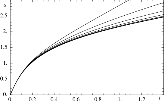
Figure 1: Expansion parameter $a$ as a function of $t$ for the case $\text{M}\Lambda w$ with $\lambda=1$, $\rho_{\text{i}}=10$, $\epsilon_{\text{i}}=200$. Curves are for $w$ from $-1$ to $1$ with step $0.2$ from top to bottom.

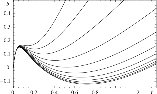
Figure 2: Expansion parameter $b$ as a function of $t$ for the case $\text{M}\Lambda w$ with $\lambda=1$, $\rho_{\text{i}}=10$, $\epsilon_{\text{i}}=200$. Curves are for $w$ from $-1$ to $1$ with step $0.2$ from top to bottom.

Figure 3: Matter density $\rho$ as a function of $t$ for the case $\text{M}\Lambda w$ with $\lambda=1$, $\rho_{\text{i}}=10$, $\epsilon_{\text{i}}=200$. Curves are for $w$ from $-1$ to $1$ with step $0.2$ from top to bottom.

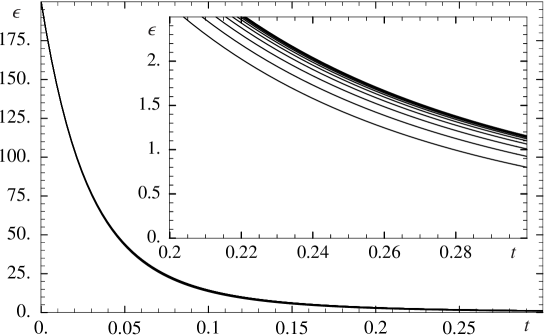
Figure 4: Magnetic field density $\epsilon$ as a function of $t$ for the case $\text{M}\Lambda w$ with $\lambda=1$, $\rho_{\text{i}}=10$, $\epsilon_{\text{i}}=200$. Curves are for $w$ from $-1$ to $1$ with step $0.2$ from bottom to top.

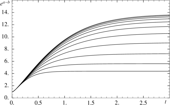
Figure 5: Pseudo-eccentricity $e^{a-b}$ for the case $\text{M}\Lambda w$ with $\lambda=1$, $\rho_{\text{i}}=10$, $\epsilon_{\text{i}}=200$. Curves are for $w$ from $-1$ to $1$ with step $0.2$ from bottom to top.

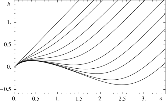
Figure 6: Expansion parameters $a$ and $b$ for the case $\text{M}\Lambda$ with $\lambda=1$, $\rho_{\text{i}}=0$. Curves are for $\epsilon_{\text{i}}=0,1,2,5,10,20,50,100,200,500,1000$ from top to bottom.

Figure 7: Asymptotic value of the pseudo-eccentricity for the case $\text{M}\Lambda w$ with $\lambda=1$ as a function of $\rho_{\text{i}}$ and $\epsilon_{\text{i}}$. Sets of curves are for $\textrm{e}^{a-b}$ equal to $20,15,10,5$ from top to bottom; the abscissa corresponds to $\textrm{e}^{a-b}=1$. Curves in each set are for $w$ equal to $-0.5,-0.25,0,0.25,0.5$ from top to bottom.

Figure 8: Asymptotic value of the pseudo-eccentricity for the case $\text{M}\Lambda w$ with $\lambda=1$ as a function of $w$ and $\rho_{\text{i}}$ for $\epsilon_{\text{i}}=200$. Curves are for $\textrm{e}^{a-b}$ from $4$ to $22$ with step $2$ from top to bottom.

In the following, we will refer to the parameters $a$ and $b$ as planar and axial expansion parameters. Note that in order to generate the figures, we have used large values for the initial matter density, $\rho_{\textrm{i}}$ and the magnetic field energy density $\epsilon_{\textrm{i}}$ relative to the cosmological constant $\lambda$ in order to make the effects of their contributions to the stress energy tensor stand out in the graphics. We will do this throughout the paper, but caution the reader that we are not implying these are realistic choices of parameters. A realistic choice of initial conditions would probably be $\lambda$, $\rho_{\textrm{i}}$, and $\epsilon_{\textrm{i}}$ all of the same order of magnitude, but in this case we would need to plot small differences of parameters instead of plotting them directly. Recall that the $\delta\rho/\rho$ effects found in the cosmic microwave background density perturbations are of order $10^{-5}$, so observationally one is typically, but not always, looking for small effects.

Figure 1 gives the expansion parameter $a$ as a function of time in a universe filled with aligned magnetic fields, cosmological constant, and matter. Each curve corresponds to matter with a different equation of state parameter $w$.

Each curve in Figure 2 plots the axial expansion parameter $b$ with time in a universe filled with aligned magnetic fields and cosmological constant for matter with a variety of choices for $w$. Comparing Figs. 1 and 2 shows $a$ grows faster than $b$. This implies the expansion is oblate, i. e., an initial spherical region expands to an oblate spheroid.

Figures 3 and 4 show the decay of the matter density and of the magnetic field energy respectively, with time using the same initial parameters that were used to generate Figs. 1 and 2. Figure 5 shows the behavior of the pseudo-eccentricity with time, again for the same initial parameters which were used in the previous figures.

In Fig. 6 we have plotted the axial expansion parameter versus the planar expansion parameter. Each curve is for a different value of initial magnetic field energy density. Time increases along each curve from left to right. Note that $a$ always increases, but for sufficiently strong initial magnetic fields, after an initial increase, $b$ reaches a maximum, then decreases for a time, reaches a minimum, and then increases thereafter. Figure 7 shows the asymptotic values of the pseudo-eccentricity as a function of magnetic field energy density and initial matter density for various fixed values of $w$. As expected, stronger $\epsilon_{\textrm{i}}$ leads to higher eccentricity, but increasing $\rho_{\textrm{i}}$, the spherically symmetric component of ${T^{\mu}}_{\nu}$ tends to dampen the effect. As with previous figures, the parameters in Figs. 6 and 7 were chosen to enhance the visualization, not for physical reasons. Finally, Fig. 8 is a contour plot of the asymptotic value of the pseudo-eccentricity (the curves are lines of equal asymptotic value of $e^{a-b}$) for a range of initial matter densities and equations of state.

V Strings

In a somewhat artificial case of cosmological constant plus strings plus matter, the equations to solve are

$$\dot{a}^{2}+2\dot{a}\dot{b}=\lambda+\rho+\epsilon,$$ (56)

$$2\ddot{a}+3\dot{a}^{2}=\lambda-w\rho+\epsilon,$$ (57)

$$\dot{\epsilon}+2\dot{a}\epsilon=0.$$ (58)

From the conservation of the anisotropic part of the energy-momentum, Eq. (58), we find

$$a={\textstyle{\frac{1}{2}}}\ln{(\epsilon_{\textrm{i}}/\epsilon)}.$$ (59)

Proceeding with the analysis in a matter similar to Sec. IV, we arrive at the following system of equations:

$$\epsilon f^{\prime}-{\textstyle{\frac{7}{2}}}f+\epsilon^{2}(\lambda-w\rho+\epsilon)=0,$$ (60)

$$\epsilon f\rho^{\prime}-(1+w)\rho\left[{\textstyle{\frac{3}{4}}}f+{\textstyle{\frac{1}{2}}}\epsilon^{2}(\lambda+\rho+\epsilon)\right]=0,$$ (61)

or equivalently

$$f={\textstyle{\frac{2}{3}}}\lambda\epsilon^{2}+2\epsilon^{3}+{\textstyle{\frac{2}{3}}}\epsilon_{\textrm{i}}^{-\frac{3}{2}}(\rho_{\textrm{i}}-2\epsilon_{\textrm{i}})\epsilon^{\frac{7}{2}}-w\epsilon^{\frac{7}{2}}\int_{\epsilon}^{\epsilon_{\textrm{i}}}\textrm{d}\epsilon\,\rho\epsilon^{-\frac{5}{2}},$$ (62)

$$\rho=\rho_{\textrm{i}}(\epsilon/\epsilon_{\textrm{i}})^{\frac{3}{4}(1+w)}\psi\left[1+{\textstyle{\frac{1}{2}}}(1+w)\rho_{\textrm{i}}\epsilon_{\textrm{i}}\int_{\epsilon}^{\epsilon_{\textrm{i}}}\textrm{d}\epsilon\,(\epsilon/\epsilon_{\textrm{i}})^{1+\frac{3}{4}(1+w)}\psi f^{-1}\right]^{-1},$$ (63)

where

$$\psi=\exp{\left[-{\textstyle{\frac{1}{2}}}(1+w)\int_{\epsilon}^{\epsilon_{\textrm{i}}}\textrm{d}\epsilon\,\epsilon(\lambda+\epsilon)f^{-1}\right]}.$$ (64)

As in the magnetic field case, we can find the exact solution to the coupled system of equations only for non-relativistic matter ($w=0$), which we present below. An approximate solution for arbitrary $w$ together with large $t$ asymptotics are given in Appendix B. Setting $w=0$, Eqs. (62) and (63) reduce to

$$f={\textstyle{\frac{2}{3}}}\lambda\epsilon^{2}+2\epsilon^{3}+{\textstyle{\frac{2}{3}}}\epsilon_{\textrm{i}}^{-\frac{3}{2}}(\rho_{\textrm{i}}-2\epsilon_{\textrm{i}})\epsilon^{\frac{7}{2}},$$ (65)

$$\rho=\rho_{\textrm{i}}(\epsilon/\epsilon_{\textrm{i}})^{\frac{3}{2}}\left[1+F(\epsilon/\epsilon_{\textrm{i}})\right]^{-1}\left[\frac{\lambda+3\epsilon+(\rho_{\textrm{i}}-2\epsilon_{\textrm{i}})(\epsilon/\epsilon_{\textrm{i}})^{\frac{3}{2}}}{\lambda+\rho_{\textrm{i}}+\epsilon_{\textrm{i}}}\right]^{-\frac{1}{2}},$$ (66)

where

$$F(\epsilon/\epsilon_{\textrm{i}})={\textstyle{\frac{3}{4}}}(\rho_{\textrm{i}}/\epsilon_{\textrm{i}})[1+(\lambda+\rho_{\textrm{i}})/\epsilon_{\textrm{i}}]^{\frac{1}{2}}\int_{\epsilon/\epsilon_{\textrm{i}}}^{1}\textrm{d}x\,x^{\frac{1}{2}}\left\{\lambda/\epsilon_{\textrm{i}}+3x+(\rho_{\textrm{i}}/\epsilon_{\textrm{i}}-2)x^{\frac{3}{2}}\right\}^{-\frac{3}{2}}.$$ (67)

Equations (11), (59) and (66) give

$$b={\textstyle{\frac{1}{2}}}\ln\frac{\lambda+3\epsilon+(\rho_{\textrm{i}}-2\epsilon_{\textrm{i}})(\epsilon/\epsilon_{\textrm{i}})^{\frac{3}{2}}}{\lambda+\rho_{\textrm{i}}+\epsilon_{\textrm{i}}}-{\textstyle{\frac{1}{2}}}\ln{(\epsilon/\epsilon_{\textrm{i}})}+\ln\left[1+F(\epsilon/\epsilon_{\textrm{i}})\right].$$ (68)

The time dependences of the above functions $\rho(\epsilon)$, $a(\epsilon)$ and $b(\epsilon)$ are found from the function $\epsilon(t)$ which is given implicitly by

$$t-t_{\textrm{i}}={\textstyle{\frac{1}{2}}}\int^{\epsilon_{\textrm{i}}}_{\epsilon}\textrm{d}\epsilon\left[{\textstyle{\frac{1}{3}}}\lambda\epsilon^{2}+\epsilon^{3}+{\textstyle{\frac{1}{3}}}\epsilon_{\textrm{i}}^{-\frac{3}{2}}(\rho_{\textrm{i}}-2\epsilon_{\textrm{i}})\epsilon^{\frac{7}{2}}\right]^{-\frac{1}{2}}.$$ (69)

There is a substantial analogy with the magnetic field case: all the statements in the paragraph following Eq. (41) in Sec. IV are also correct for the case of strings if one replaces the magnetic field density with the string density.

In the case $w=0$, asymptotics from Appendix B simplify as follows:

$$\epsilon\sim\epsilon_{\textrm{i}}\,\exp\left[-2(\lambda/3)^{\frac{1}{2}}(t-t_{\textrm{i}}+\tau)\right],$$ (70)

$$a\sim(\lambda/3)^{\frac{1}{2}}(t-t_{\textrm{i}}+\tau),$$ (71)

$$b\sim(\lambda/3)^{\frac{1}{2}}(t-t_{\textrm{i}}+\tau)-{\textstyle{\frac{1}{2}}}\ln{\left[1+(\rho_{\textrm{i}}+\epsilon_{\textrm{i}})/\lambda\right]}+\ln{[1+F(0)]},$$ (72)

$$\rho\sim\rho_{\textrm{i}}\left[1+(\lambda+\rho_{\textrm{i}})/\epsilon_{\textrm{i}}\right]^{\frac{1}{2}}[1+F(0)]^{-1}\exp\left[-(3\lambda)^{\frac{1}{2}}(t-t_{\textrm{i}}+\tau)\right],$$ (73)

where

$$\tau={\textstyle{\frac{1}{2}}}\int_{0}^{\epsilon_{\textrm{i}}}\textrm{d}\epsilon\left\{\left({\textstyle{\frac{1}{3}}}\lambda\epsilon^{2}\right)^{-\frac{1}{2}}-\left[{\textstyle{\frac{1}{3}}}\lambda\epsilon^{2}+\epsilon^{3}+{\textstyle{\frac{1}{3}}}\epsilon_{\textrm{i}}^{-\frac{3}{2}}(\rho_{\textrm{i}}-2\epsilon_{\textrm{i}})\epsilon^{\frac{7}{2}}\right]^{-\frac{1}{2}}\right\}.$$ (74)

The corresponding asymptotic for the pseudo-eccentricity is

$$\textrm{e}^{a-b}\sim\left[1+(\rho_{\textrm{i}}+\epsilon_{\textrm{i}})/\lambda\right]^{\frac{1}{2}}\left[1+F(0)\right]^{-1}.$$ (75)

To find the lower bound for this quantity, we replace the expression in the braces in Eq. (67) by its bound, $\lambda/\epsilon_{\textrm{i}}+(1+\rho_{\textrm{i}}/\epsilon_{\textrm{i}})x^{\frac{3}{2}}$, integrate, and find

$$\textrm{e}^{a-b}\gtrsim\left[\frac{\rho_{\textrm{i}}}{\rho_{\textrm{i}}+\epsilon_{\textrm{i}}}+\frac{\epsilon_{\textrm{i}}}{\rho_{\textrm{i}}+\epsilon_{\textrm{i}}}\left(1+\frac{\rho_{\textrm{i}}+\epsilon_{\textrm{i}}}{\lambda}\right)^{-\frac{1}{2}}\right]^{-1}\geq 1.$$ (76)

This is the same bound we found for the magnetic field case [Eq. (48)], and we see the expansion is again of the oblate form.

Again, for the case $\lambda=0$, the above solution is given in terms of elementary functions. We find

$$F(\epsilon/\epsilon_{\textrm{i}}) = (\rho_{\textrm{i}}/\epsilon_{\textrm{i}})\theta(1)\left\{\frac{1}{\theta(1)}-\frac{1}{\theta(\epsilon/\epsilon_{\textrm{i}})}-\textrm{\,arctanh\,}{\theta(1)}+\textrm{\,arctanh\,}{\theta(\epsilon/\epsilon_{\textrm{i}})}\right\}$$ (77)

$$t-t_{\textrm{i}} = \epsilon_{\textrm{i}}^{-\frac{1}{2}}\left\{{\textstyle{\frac{1}{3}}}(\rho_{\textrm{i}}/\epsilon_{\textrm{i}}-2)\left[\textrm{\,arctanh\,}{\theta(1)}-\textrm{\,arctanh\,}{\theta(\epsilon/\epsilon_{\textrm{i}})}\right]\right.$$ (78)

$$\hskip 21.52771pt\left.-\theta(1)+(\epsilon/\epsilon_{\textrm{i}})^{-\frac{1}{2}}\theta(\epsilon/\epsilon_{\textrm{i}})\right\},$$

where

$$\theta(x)=\left[1+{\textstyle{\frac{1}{3}}}\left(\rho_{\textrm{i}}/\epsilon_{\textrm{i}}-2\right)x^{\frac{1}{2}}\right]^{\frac{1}{2}}.$$ (79)

The large-time asymptotics are

$$\epsilon\sim\epsilon_{\textrm{i}}f^{-2}(t),$$ (80)

$$a\sim f(t),$$ (81)

$$b\sim-f(t),$$ (82)

$$\rho\sim\rho_{\textrm{i}}\textrm{e}^{-f(t)},$$ (83)

where $f(t)=t\epsilon_{\textrm{i}}^{\frac{1}{2}}+{\textstyle{\frac{1}{6}}}(\rho_{\textrm{i}}/\epsilon_{\textrm{i}}-2)\ln{(t\epsilon_{\textrm{i}}^{\frac{1}{2}})}$. The pseudo-eccentricity becomes

$$\textrm{e}^{a-b}\sim\textrm{e}^{2f(t)}.$$ (84)

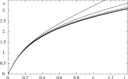
Figure 9: Expansion parameter $a$ as a function of $t$ for the case $\text{S}\Lambda w$ with $\lambda=1$, $\rho_{\text{i}}=10$, $\epsilon_{\text{i}}=200$. Curves are for $w$ from $-1$ to $1$ with step $0.2$ from top to bottom.

Figure 10: Expansion parameter $b$ as a function of $t$ for the case $\text{S}\Lambda w$ with $\lambda=1$, $\rho_{\text{i}}=10$, $\epsilon_{\text{i}}=200$. Curves are for $w$ from $-1$ to $1$ with step $0.2$ from top to bottom.

Figure 11: Matter density $\rho$ as a function of $t$ for the case $\text{S}\Lambda w$ with $\lambda=1$, $\rho_{\text{i}}=10$, $\epsilon_{\text{i}}=200$. Curves are for $w$ from $-1$ to $1$ with step $0.2$ from top to bottom.

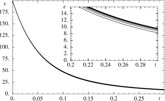
Figure 12: Magnetic field density $\epsilon$ as a function of $t$ for the case $\text{S}\Lambda w$ with $\lambda=1$, $\rho_{\text{i}}=10$, $\epsilon_{\text{i}}=200$. Curves are for $w$ from $-1$ to $1$ with step $0.2$ from bottom to top.

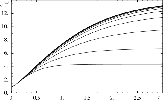
Figure 13: Pseudo-eccentricity $e^{a-b}$ for the case $\text{S}\Lambda w$ with $\lambda=1$, $\rho_{\text{i}}=10$, $\epsilon_{\text{i}}=200$. Curves are for $w$ from $-1$ to $1$ with step $0.2$ from bottom to top.

Figure 14: Expansion parameters $a$ and $b$ for the case $\text{S}\Lambda$ with $\lambda=1$, $\rho_{\text{i}}=0$. Curves are for $\epsilon_{\text{i}}=0,1,2,5,10,20,50,100,200,500,1000$ from top to bottom.

Figure 15: Asymptotic value of the pseudo-eccentricity for the case $\text{S}\Lambda w$ with $\lambda=1$ as a function of $\rho_{\text{i}}$ and $\epsilon_{\text{i}}$. Sets of curves are for $\textrm{e}^{a-b}$ equal to $20,15,10,5$ from top to bottom; the abscissa corresponds to $\textrm{e}^{a-b}=1$. Curves in each set are for $w$ equal to $-0.5,-0.25,0,0.25,0.5$ from top to bottom.

Figure 16: Asymptotic value of the pseudo-eccentricity for the case $\text{S}\Lambda w$ with $\lambda=1$ as a function of $w$ and $\rho_{\text{i}}$ for $\epsilon_{\text{i}}=200$. Curves are for $\textrm{e}^{a-b}$ from $4$ to $22$ with step $2$ from top to bottom.

Figures 9 and 10 plot $a$ and $b$ as a function of time for a range of $w$ values. While Fig. 9 is qualitatively similar to Fig. 1, Fig. 10 shows only a monotonic increase in $b$, unlike Fig. 2. (See 2, 4 in Sec. III.) Figures 11 and 12 show the matter density and string density as a function of time. These figures are qualitatively similar to Figs. 3 and 4 for the magnetic field case, but the curves in the string case are somewhat more compressed. Figure 13 is the plot of the pseudo-eccentricity with time for strings. Figure 14 plots $a$ versus $b$ for a variety of values of initial string density. The monotonic increase of $b$ is again apparent, in contrast to the results for magnetic fields shown in Fig. 6.

Figure 15 gives contours of asymptotic values of the pseudo-eccentricity as a function of matter density and string density. The results are similar, but somewhat milder than the magnetic case, Fig. 7. Finally, Fig. 16. shows a dependence of the asymptotic value of the pseudo-eccentricity on the equation of state. The effect is again similar to, but milder than, the magnetic field case.

VI Walls

If we replace magnetic fields or cosmic strings from the previous two sections by a uniform stack of cosmic domain walls, we arrive at another solvable model described by the following equations:

$$\dot{a}^{2}+2\dot{a}\dot{b}=\lambda+\rho+\epsilon,$$ (85)

$$2\ddot{a}+3\dot{a}^{2}=\lambda-w\rho,$$ (86)

$$\dot{\epsilon}+\dot{b}\epsilon=0.$$ (87)

Again, we were not able to solve the above equations exactly for arbitrary $w$; also, it appears to be much harder to arrive at a simple and accurate approximation similar to the approximations for the cases of magnetic fields and strings (see Appendices A and B for details). We reluctantly restrict ourselves only to the case $w=0$. Somewhat surprisingly, the analysis will need to be substantially different from the magnetic fields and strings cases.

To proceed, it is convenient to use the substitution $a=\frac{2}{3}\ln{u}$, which transforms the Riccati Eq. (86) into an easily solvable linear equation $\ddot{u}={\textstyle{\frac{3}{4}}}\lambda u$. This results in

$$a={\textstyle{\frac{2}{3}}}\ln\frac{\gamma^{3}-\sigma}{1-\sigma}-\ln{\gamma},$$ (88)

where $\gamma=\exp\left[(\lambda/3)^{\frac{1}{2}}(t-t_{\textrm{i}})\right]$ and

$$\sigma=\frac{\left[1+(\rho_{\textrm{i}}+\epsilon_{\textrm{i}})/\lambda\right]^{\frac{1}{2}}-1}{\left[1+(\rho_{\textrm{i}}+\epsilon_{\textrm{i}})/\lambda\right]^{\frac{1}{2}}+1}.$$ (89)

Energy-momentum conservation, Eq. (87), gives

$$b=\ln{(\epsilon_{\textrm{i}}/\epsilon)}.$$ (90)

Using Eqs. (11), (85), (88), and (90), we find

$$\epsilon=\epsilon_{\textrm{i}}\gamma\frac{1+\sigma}{\gamma^{3}+\sigma}\left(\frac{\gamma^{3}-\sigma}{1-\sigma}\right)^{\frac{1}{3}}\left\{1+\frac{3\epsilon_{\textrm{i}}}{2\lambda}\frac{1+\sigma}{(1-\sigma)^{\frac{1}{3}}}F(\gamma)+\frac{\rho_{\textrm{i}}}{2\lambda}(1-\sigma)\frac{\gamma^{3}-1}{\gamma^{3}+\sigma}\right\}^{-1},$$ (91)

where

$$F(\gamma)=\int_{1}^{\gamma}\textrm{d}x\,\frac{(x^{3}-\sigma)^{\frac{4}{3}}}{(x^{3}+\sigma)^{2}}.$$ (92)

The function $F(\gamma)$ can be written in terms of the hypergeometric functions, but the expression is complicated and not illuminating, so we will not give it here.

In the case $\lambda=0$, the above exact solution simplifies significantly. Instead of Eq. (88) we now have

$$a={\textstyle{\frac{2}{3}}}\ln(1-C+Ct),$$ (93)

where $C=1-{\textstyle{\frac{1}{2}}}[3(\rho_{\textrm{i}}+\epsilon_{\textrm{i}})]^{\frac{1}{2}}$, and Eq. (91) becomes

$$\epsilon=\epsilon_{\textrm{i}}(1-C+Ct)^{\frac{1}{3}}\left\{1+\frac{3\rho_{\textrm{i}}}{4C}(t-t_{\textrm{i}})+\frac{9\epsilon_{\textrm{i}}}{28C^{2}}\left[(1-C+Ct)^{\frac{7}{3}}-1\right]\right\}^{-1},$$ (94)

Returning to the case of $\lambda\not=0$, the large $t$ wall energy density is

$$\epsilon\sim\epsilon_{\textrm{i}}\,\textrm{e}^{-(\lambda/3)^{\frac{1}{2}}(t-t_{\textrm{i}})}\left[\frac{(1-\sigma)^{\frac{1}{3}}}{1+\sigma}+\frac{3\epsilon_{\textrm{i}}}{2\lambda}F(\infty)+\frac{\rho_{\textrm{i}}}{2\lambda}\frac{(1-\sigma)^{\frac{4}{3}}}{1+\sigma}\right]^{-1},$$ (95)

the transverse scale factor is

$$a\sim(\lambda/3)^{\frac{1}{2}}(t-t_{\textrm{i}})-{\textstyle{\frac{2}{3}}}\ln{(1-\sigma)},$$ (96)

the longitudinal scale factor is

$$b\sim(\lambda/3)^{\frac{1}{2}}(t-t_{\textrm{i}})+\ln\left[\frac{(1-\sigma)^{\frac{1}{3}}}{1+\sigma}+\frac{3\epsilon_{\textrm{i}}}{2\lambda}F(\infty)+\frac{\rho_{\textrm{i}}}{2\lambda}\frac{(1-\sigma)^{\frac{4}{3}}}{1+\sigma}\right],$$ (97)

and the matter density is

$$\rho\sim\textrm{e}^{-(3\lambda)^{\frac{1}{2}}(t-t_{\textrm{i}})}\left[\frac{(1-\sigma)^{\frac{5}{3}}}{1+\sigma}+\frac{3\epsilon_{\textrm{i}}}{2\lambda}(1-\sigma)^{\frac{4}{3}}F(\infty)+\frac{\rho_{\textrm{i}}}{2\lambda}\frac{(1-\sigma)^{\frac{8}{3}}}{1+\sigma}\right]^{-1}.$$ (98)

From Eqs. (96) and (97) the pseudo-eccentricity is

$$\textrm{e}^{a-b}\sim\left[\frac{1-\sigma}{1+\sigma}+\frac{3\epsilon_{\textrm{i}}}{2\lambda}(1-\sigma)^{\frac{2}{3}}F(\infty)+\frac{\rho_{\textrm{i}}}{2\lambda}\frac{(1-\sigma)^{2}}{1+\sigma}\right]^{-1}.$$ (99)

In the case of zero vacuum energy, the asymptotics read:

$$\epsilon\sim\text{const}\ t^{-2},$$ (100)

$$a\sim{\textstyle{\frac{2}{3}}}\ln{t}+\text{const},$$ (101)

$$b\sim 2\ln{t}+\text{const},$$ (102)

$$\rho\sim\text{const}\ t^{-\frac{10}{3}}.$$ (103)

As opposed to the cases of magnetic fields and strings, the pseudo-eccentricity vanishes for large $t$, since $\textrm{e}^{a-b}\sim t^{-\frac{4}{3}}$.

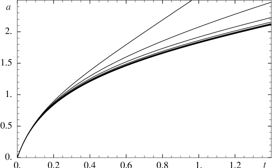
Figure 17: Expansion parameter $a$ as a function of $t$ for the case $\text{W}\Lambda w$ with $\lambda=1$, $\rho_{\text{i}}=10$, $\epsilon_{\text{i}}=200$. Curves are for $w$ from $-1$ to $1$ with step $0.2$ from top to bottom.

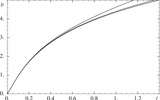
Figure 18: Expansion parameter $b$ as a function of $t$ for the case $\text{W}\Lambda w$ with $\lambda=1$, $\rho_{\text{i}}=10$, $\epsilon_{\text{i}}=200$. Curves are for $w$ from $-1$ to $1$ with step $0.2$ from top to bottom.

Figure 19: Matter density $\rho$ as a function of $t$ for the case $\text{W}\Lambda w$ with $\lambda=1$, $\rho_{\text{i}}=10$, $\epsilon_{\text{i}}=200$. Curves are for $w$ from $-1$ to $1$ with step $0.2$ from top to bottom.

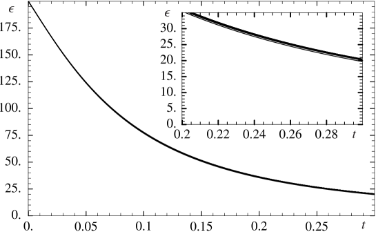
Figure 20: Magnetic field density $\epsilon$ as a function of $t$ for the case $\text{W}\Lambda w$ with $\lambda=1$, $\rho_{\text{i}}=10$, $\epsilon_{\text{i}}=200$. Curves are for $w$ from $-1$ to $1$ with step $0.2$ from bottom to top.

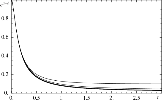
Figure 21: Pseudo-eccentricity $e^{a-b}$ for the case $\text{W}\Lambda w$ with $\lambda=1$, $\rho_{\text{i}}=10$, $\epsilon_{\text{i}}=200$. Curves are for $w$ from $-1$ to $1$ with step $0.2$ from top to bottom.

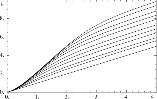
Figure 22: Expansion parameters $a$ and $b$ for the case $\text{W}\Lambda$ with $\lambda=1$, $\rho_{\text{i}}=0$. Curves are for $\epsilon_{\text{i}}=0,1,2,5,10,20,50,100,200,500,1000$ from bottom to top.

Figure 23: Asymptotic value of the pseudo-eccentricity for the case $\text{W}\Lambda w$ with $\lambda=1$ as a function of $\rho_{\text{i}}$ and $\epsilon_{\text{i}}$. Sets of curves are for $\textrm{e}^{a-b}$ equal to $0.02,0.03,0.04,0.05$ from top to bottom; the abscissa corresponds to $\textrm{e}^{a-b}=1$. Curves in each set are for $w$ equal to $-0.5,-0.25,0,0.25,0.5$ from top to bottom.

Figure 24: Asymptotic value of the pseudo-eccentricity for the case $\text{W}\Lambda w$ with $\lambda=1$ as a function of $w$ and $\rho_{\text{i}}$ for $\epsilon_{\text{i}}=200$. Curves are for $\textrm{e}^{a-b}$ from $0.0115$ to $0.0120$ with step $0.0001$ from bottom to top.

The plots for walls shows a number of qualitative differences with the previous cases of magnetic fields and strings. The expansion parameters $a$ and $b$ change with time (see Figs. 17 and 18) more like the string case, where both grow monotonically; but note that now $b$ grows faster than $a$, which is the reverse of the behavior seen for strings. This means the expansion for walls is always prolate, unlike the expansions for strings and magnetic fields which are always oblate.

For walls, the matter density, Fig. 19, falls faster with time than its string and magnetic field counterparts due to the fact that the overall expansion, and therefore density dilution, is faster for walls. On the other hand, due to the nature of its contribution to the stress energy tensor, the wall energy density, Fig. 20, falls more slowly than the magnetic field and string energy densities.

Figure 21 for the pseudo-eccentricity provides another way of visualizing the prolateness of the wall expansion, since $e^{a-b}$ is always less than one in this case. Figure 22 for $a$ versus $b$ represents the degree of prolateness for wall expansion for a variety of initial conditions. Figure 23 shows asymptotic pseudo-eccentricity contours for walls as a function of initial matter and wall energy densities, and Fig. 24 gives asymptotic pseudo-eccentricity contours for walls as a function of matter density and equation of state parameter $w$.

VII Conclusions

Einstein’s equations for magnetic fields that extend across the Universe have been considered elsewhere. Examples include cylindrically symmetric magnetic geons, exact solutions for planar geometry with magnetic fields and dust, and asymptotics magnetic-fields . None of these studies contain exact solutions with cosmological constant and magnetic fields ($\Lambda\text{M}$). We have not only given exact solutions to the $\Lambda\text{M}$ case, but also have found exact $\Lambda\text{M}$ plus dust solutions. In addition we have exact solutions when the magnetic fields are replaced by uniform arrangements of cosmic strings or cosmic domain walls. Finally we have given approximate solutions in all these cases where dust can be replaced by matter with an arbitrary value of $w$ in its equation of state. All our solutions have planar symmetry.

The cosmic microwave background (CMB) and other modern cosmological data are of such high quality that it is now possible to study aspects of the Universe that were previously completely out of reach. In order to carry out these investigations, it may be necessary to go beyond the homogeneous isotropic big bang/inflationary cosmology and compare the data with less symmetric but perhaps more realistic models. In the case of planar symmetry studied here, an understanding of the density perturbations and structure formation requires perturbing around planar symmetric solutions. Here we have taken a step in that direction by considering a planar symmetric universe with eccentric expansion, and have shown exact solutions can be obtained even when the eccentricity is large. This will allow a density perturbation analysis to be carried out in these cosmologies, which in turn can be compared with CMB data and galaxy structure and correlation data EccIII .

It is not just a mathematical exercise to consider planar symmetry. We know that magnetic fields and cosmic defects can be produced in the early universe. In the case of magnetic fields, their energy density $\epsilon$ at its production epoch can be a substantial fraction of the matter density $\rho$, and this can cause spherical symmetry to be lost in a cosmology. If the typical magnetic domain size $D$ is small compared to $H^{-1}$, then the local expansion is eccentric, while the average global expansion remains spherical, while if $D\geq H^{-1}$, then the whole universe expands eccentrically until $D$ comes within the horizon. Also, if $D\leq H^{-1}$ initially, a period of inflation can push regions of size $D$ outside the horizon, and we are again in a situation of eccentric expansion.

The planar symmetric cases of cosmic strings and domain walls are somewhat more artificial, since they are assumed to be static and aligned. However, this may not be totally unrealistic when considered from the perspective of more fundamental theories. For instance, certain AdS/CFT theories derived from string theory have parallel walls, and other theories with branes can have strings connecting them. If two parallel walls, both outside the horizon, were connected by strings, then the strings would be expected to be parallel on average even if they had some dynamics. Based on the above remarks, and with the knowledge of the fact that aligned walls and strings both produce planar symmetry, we have given exact solutions for these cases as well.

Even though magnetic fields, string, and wall systems all have planar symmetry, the form of their energy momentum tensors differ. For magnetic fields, ${T^{\mu}}_{\nu}$ is traceless, and so this case has similarities with a radiation filled universe. For strings and walls, the trace of ${T^{\mu}}_{\nu}$ does not vanish, so there are some similarities with the non-relativistic matter component. Strings and walls are under tension, so they also have some similarities with vacuum energy. To see all these properties, we have solved the equations of motion exactly for many cases of interest. The large-time behaviors of these solutions are summarized in Table 3.

Table 3: Summary of large-time behavior for various quantities for ten different cases of universe content. For each choice of an anisotropic component, magnetic fields (M), strings (S) or walls (W), matter with $w=0$ or with $0<w<1$ is included and cosmological constant is either present ($\Lambda$) or absent. Only the leading terms in asymptotics are given and $\tilde{t}=(\lambda/3)^{\frac{1}{2}}t$.

	$\epsilon$	$\rho$	$\textrm{e}^{a}$	$\textrm{e}^{b}$	$\textrm{e}^{a-b}$
$\text{M}\Lambda w$	$\textrm{e}^{-4\tilde{t}}$	$\textrm{e}^{-3(1+w)\tilde{t}}$	$\textrm{e}^{\tilde{t}}$	$\textrm{e}^{\tilde{t}}$	$\geq 1$
$\text{M}\Lambda 0$	$\textrm{e}^{-4\tilde{t}}$	$\textrm{e}^{-3\tilde{t}}$	$\textrm{e}^{\tilde{t}}$	$\textrm{e}^{\tilde{t}}$	$\geq 1$
$\text{M}w$	$t^{-\frac{8}{3}}$	$t^{-2}$	$t^{\frac{2}{3}}$	$t^{\frac{2(1-2w)}{3(1+w)}}$	$t^{\frac{2w}{1+w}}$
$\text{M}0$	$t^{-\frac{8}{3}}$	$t^{-2}$	$t^{\frac{2}{3}}$	$t^{\frac{2}{3}}$	$\geq 1$
$\text{S}\Lambda w$	$\textrm{e}^{-2\tilde{t}}$	$\textrm{e}^{-3(1+w)\tilde{t}}$	$\textrm{e}^{\tilde{t}}$	$\textrm{e}^{\tilde{t}}$	$\geq 1$
$\text{S}\Lambda 0$	$\textrm{e}^{-2\tilde{t}}$	$\textrm{e}^{-3\tilde{t}}$	$\textrm{e}^{\tilde{t}}$	$\textrm{e}^{\tilde{t}}$	$\geq 1$
$\text{S}w$	$t^{-2}$	$t^{-2}$	$t$	$t^{-\frac{2w}{1+w}}$	$t^{\frac{1+3w}{1+w}}$
$\text{S}0$	$t^{-2}$	$t^{-2}$	$t$	$t^{-2}$	$\geq 1$
$\text{W}\Lambda 0$	$\textrm{e}^{-\tilde{t}}$	$\textrm{e}^{-3\tilde{t}}$	$\textrm{e}^{\tilde{t}}$	$\textrm{e}^{\tilde{t}}$	$\leq 1$
$\text{W}0$	$t^{-2}$	$t^{-\frac{10}{3}}$	$t^{\frac{2}{3}}$	$t^{2}$	$t^{-\frac{4}{3}}$

In all these cases, the universe undergoes eccentric expansion and in some instances eccentric inflation. Our analysis is completely general, and in order to apply these results, more input is necessary, e. g., initial conditions need to be specified, perhaps as derived from a model with early universe phase transitions. Time scales need to be fixed, e. g., when did the phase transition take place? For instance, for magnetic field production, a phase transition not far above the electroweak scale may be effective in producing eccentric effects and at the same time remaining compatible with other requirements on the cosmological model, e. g., successful baryogeneses. If the magnetic field production scale were too high, then there is a danger that all the eccentric effects could be washed out.

As stated above, with exact planar symmetric solutions at hand, we are now in a position to begin density perturbations analysis EccIII . To apply the results of this paper, it will be necessary to consider how the spectrum of density perturbations are effected by asymmetric expansion. Since perturbations get laid down by quantum fluctuations and then asymmetrically expanded in our models, any initial spherical perturbation becomes ellipsoidal. After a while, the expansion becomes spherically symmetric again, but as long as perturbations remain outside the horizon they stay ellipsoidal. Only after they reenter our horizon will they be able to adjust (they will probably start to oscillate between prolate and oblate with frequency that depends on size and overdensity). So if the perturbations are just entering at last scattering they should be ellipsoidal. The smaller they are at last scattering, the more they have oscillated and if damped, the closer to spherical they should be. Hence, the larger scale perturbations (corresponding to smaller $\ell$) will have a better memory of the eccentric phase. This would appear to agree with what seems to be hinted at in the WMAP observations: more distortion of the low $\ell$ modes. However, a detailed phenomenological analysis needs to be carried out to confirm these facts.

To summarize, what we need are modes that expanded eccentrically to be entering the horizon at the time of last scattering and then to feed this information into a Sachs-Wolfe type of calculation. This is a most interesting and challenging calculation, since it requires a full reanalysis of the density perturbations in eccentric geometry. In this paper we have moved toward this goal. We have carried out exact calculations of the evolution of a variety of Universes with asymmetric matter content. In some cases, namely when $w$ is neither zero nor minus one, we have been forced to use approximate methods. We have explored the asymptotic behavior of both the exact and approximate cases. Our results provide a starting point for the analysis of density perturbations in asymmetric cosmologies. WMAP and its successors will be able to either bound or detect effects of asymmetric inflation and we have taken the first steps in the theoretical exploration in that direction.

Finally, we make a few comments about the case where there are multiple magnetic domains within the cosmological horizon. (A similar discussion would apply to strings and walls.) If the domains are randomly oriented then what one should expect is eccentric expansion within each domain, with dependence on the local value of the cosmological constant, magnetic field strength, and matter content. Locally there is planar symmetry, but globally the Universe would look isotropic if averaged over many domains. One effect of the averaging would be an alteration of the power spectrum on scales of order of the domain size. This assumes the domains have a preferred size, that is probably on order of the horizon size when they were produced, if the associated phase transition was second order, or on the size of the correlation length at production, if the associated phase transition was first order. This is in contrast to the density perturbations produced in inflation that typically have a flat power spectrum. One would also expect to see polarization effects to survive in the CMB in an isotropic average of magnetic domains. A detailed analysis of these effects would take dedicated numerical studies.

Appendix A Approximate solutions for $\bm{\Lambda}+\text{M}+\text{MATTER}$ with arbitrary $w$

We develop a simple approximation by expanding around $\epsilon=0$. Eliminating $\rho$ in Eqs. (32) and (33), we find

$$2wf\frac{\epsilon^{2}f^{\prime\prime}-\frac{15}{4}\epsilon f^{\prime}+\frac{11}{2}f+2\epsilon^{3}}{\epsilon f^{\prime}-{\textstyle{\frac{11}{4}}}f+2\epsilon^{2}(\lambda+\epsilon)}=(1+w)\left[\epsilon f^{\prime}-{\textstyle{\frac{1}{4}}}(11-3w)f+2(1+w)\epsilon^{2}(\lambda+\epsilon)\right].$$ (104)

A power series solution in $\epsilon$ to this equation is

$$f\approx{\textstyle{\frac{8}{3}}}\lambda\epsilon^{2}+{\textstyle{\frac{8}{3}}}\epsilon_{\textrm{i}}^{-\frac{3}{4}}\left[\rho_{\textrm{i}}(\epsilon/\epsilon_{\textrm{i}})^{\frac{3}{4}w}+4\epsilon_{\textrm{i}}\right]\epsilon^{\frac{11}{4}}-8\epsilon^{3}+{\cal O}\left[\epsilon^{\frac{1}{4}(15+3w)}\right].$$ (105)

The approximate solution for $\rho(\epsilon)$ can then be found from Eqs. (35) and (36). [A much faster way to calculate $\rho$ is to use Eq. (32) directly. The result, $\rho\approx\rho_{\textrm{i}}(\epsilon/\epsilon_{\textrm{i}})^{\frac{3}{4}(1+w)}$, is unacceptably inaccurate as is clear from both the exact solution (38) for $w=0$ and the asymptotic form (109) below for arbitrary $w$.] The functions $a(\epsilon)$ and $b(\epsilon)$ are given by Eqs. (30) and (11). Finally, time dependence of the above functions $\rho(\epsilon)$, $a(\epsilon)$ and $b(\epsilon)$ can be deduced from the function $\epsilon(t)$, which is given implicitly by

$$t-t_{\textrm{i}}\approx{\textstyle{\frac{1}{4}}}\int^{\epsilon_{\textrm{i}}}_{\epsilon}\textrm{d}\epsilon\left\{{\textstyle{\frac{1}{3}}}\lambda\epsilon^{2}+{\textstyle{\frac{1}{3}}}\epsilon_{\textrm{i}}^{-\frac{3}{4}}\left[\rho_{\textrm{i}}(\epsilon/\epsilon_{\textrm{i}})^{\frac{3}{4}w}+4\epsilon_{\textrm{i}}\right]\epsilon^{\frac{11}{4}}-\epsilon^{3}\right\}^{-\frac{1}{2}}$$ (106)

as it follows from $f={\textstyle{\frac{1}{2}}}\dot{\epsilon}^{2}$ and Eq. (105).

Comparing Eqs. (37) and (105), we notice that the above approximate solution becomes exact for $w=0$. In addition, being an expansion in small $\epsilon$, the approximate solution gives correct asymptotics for large $t$. To find the behavior of various quantities for large $t$, we need the corresponding asymptotic of the integral in Eq. (106). When $\lambda>0$, the integral diverges for small $\epsilon$, and so we extract this divergent part first; this results in

$$t-t_{\textrm{i}}\approx{\textstyle{\frac{1}{4}}}(3/\lambda)^{\frac{1}{2}}\ln{(\epsilon_{\textrm{i}}/\epsilon)}-\tau,$$ (107)

where

$$\tau={\textstyle{\frac{1}{4}}}\int_{0}^{\epsilon_{\textrm{i}}}\textrm{d}\epsilon\left\{\left({\textstyle{\frac{1}{3}}}\lambda\epsilon^{2}\right)^{-\frac{1}{2}}-\left[{\textstyle{\frac{1}{3}}}\lambda\epsilon^{2}+{\textstyle{\frac{1}{3}}}\epsilon_{\textrm{i}}^{-\frac{3}{4}}(\rho_{\textrm{i}}(\epsilon/\epsilon_{\textrm{i}})^{\frac{3}{4}w}+4\epsilon_{\textrm{i}})\epsilon^{\frac{11}{4}}-\epsilon^{3}\right]^{-\frac{1}{2}}\right\}.$$ (108)

Similarly extracting the divergent part of $\psi$ for small $\epsilon$, we find

$$\rho\sim(\epsilon/\epsilon_{\textrm{i}})^{\frac{3}{8}(1+w)}\textrm{e}^{(1+w)\phi}\left[1+F(0)\right]^{-1},$$ (109)

where

$$\phi=-{\textstyle{\frac{3}{8}}}(\epsilon_{\textrm{i}}/\lambda)+\int_{0}^{\epsilon_{\textrm{i}}}\textrm{d}\epsilon\,\epsilon(\lambda+\epsilon)\left\{\left({\textstyle{\frac{8}{3}}}\lambda\epsilon^{2}\right)^{-1}-f^{-1}\right\},$$ (110)

$$F(0)=(1+w)\rho_{\textrm{i}}\epsilon_{\textrm{i}}\int_{0}^{\epsilon_{\textrm{i}}}\textrm{d}\epsilon\,(\epsilon/\epsilon_{\textrm{i}})^{1+\frac{3}{8}(1+w)}\psi f^{-1}.$$ (111)

Finally, this results in the following asymptotics:

$$\epsilon\sim\epsilon_{\textrm{i}}\,\textrm{e}^{-4\sigma},$$ (112)

$$a\sim\sigma,$$ (113)

$$b\sim\sigma-\phi+(1+w)^{-1}\ln\left[1+F(0)\right],$$ (114)

$$\rho\sim\rho_{\textrm{i}}[1+F(0)]^{-1}\exp\left[-(1+w)(3\sigma-\phi)\right],$$ (115)

where $\sigma(t)=(\lambda/3)^{\frac{1}{2}}(t-t_{\textrm{i}}+\tau)$. For large $t$, both scale factors grow linearly (as in the isotropic case driven by the cosmological constant only). Due to anisotropy introduced by the magnetic fields, however, the space has expanded more transversally than longitudinally. This difference is characterized by the pseudo-eccentricity whose asymptotic form in this case is

$$\textrm{e}^{a-b}\sim\textrm{e}^{\phi}\left[1+F(0)\right]^{-1/(1+w)}.$$ (116)

When $\lambda=0$, the asymptotics depend on the range of the parameter $w$; in the most interesting case, $0<w<1$, they are:

$$\epsilon\sim 3^{-\frac{4}{3}}\epsilon_{\textrm{i}}^{-\frac{1}{3}}t^{-\frac{8}{3}},$$ (117)

$$a\sim{\textstyle{\frac{2}{3}}}\ln{(\epsilon_{\textrm{i}}^{\frac{1}{2}}t)},$$ (118)

$$b\sim\frac{2(1-2w)}{3(1+w)}\ln{(\epsilon_{\textrm{i}}^{\frac{1}{2}}t)},$$ (119)

$$\rho\sim\frac{4(1-w)}{3(1+w)}t^{-2}.$$ (120)

Thus, in the absence of constant negative pressure from the cosmological constant, anisotropy causes the space to infinitely expand in the transverse directions and infinitely contract in the longitudinal direction. This results in pseudo-eccentricity diverging for large $t$: $\textrm{e}^{a-b}\sim(\epsilon_{\textrm{i}}^{\frac{1}{2}}t)^{2w/(1+w)}$. In the case of dust ($w=0$), the asymptotic value for the pseudo-eccentricity is finite, in agreement with Eq. (55).

Appendix B Approximate solutions for $\bm{\Lambda}+\text{S}+\text{MATTER}$ with arbitrary $w$

Eliminating $\rho$ in Eqs. (60) and (61), we find

$$2wf\frac{\epsilon^{2}f^{\prime\prime}-{\textstyle{\frac{9}{2}}}\epsilon f^{\prime}+7f+\epsilon^{3}}{\epsilon f^{\prime}-{\textstyle{\frac{7}{2}}}f+\epsilon^{2}(\lambda+\epsilon)}=(1+w)\left[\epsilon f^{\prime}-{\textstyle{\frac{1}{2}}}(7-3w)f+(1+w)\epsilon^{2}(\lambda+\epsilon)\right].$$ (121)

A power series solution to this equation is

$$f={\textstyle{\frac{2}{3}}}\lambda\epsilon^{2}+2\epsilon^{3}+{\textstyle{\frac{2}{3}}}\epsilon_{\textrm{i}}^{-\frac{3}{2}}\left[\rho_{\textrm{i}}(\epsilon/\epsilon_{\textrm{i}})^{\frac{3}{2}w}-2\epsilon_{\textrm{i}}\right]\epsilon^{\frac{7}{2}}+{\cal O}\left[\epsilon^{\frac{1}{2}(9+3w)}\right]$$ (122)

The approximate solution for $\rho$ can then be found from Eqs. (63) and (64). [As in the previous section, a simple expression $\rho\approx\rho_{\textrm{i}}(\epsilon/\epsilon_{\textrm{i}})^{\frac{3}{2}(1+w)}$, which follows directly from Eq. (32), is a poor approximation.] Similar to the case of magnetic fields, the approximate solution (122) becomes exact for $w=0$.

Proceeding similarly to Appendix A, we find the following large-time asymptotics:

$$\epsilon\sim\epsilon_{\textrm{i}}\,\textrm{e}^{-2\sigma},$$ (123)

$$a\sim\sigma,$$ (124)

$$b\sim\sigma-\phi+(1+w)^{-1}\ln\left[1+F(0)\right],$$ (125)

$$\rho\sim\rho_{\textrm{i}}[1+F(0)]^{-1}\exp\left[-(1+w)(3\sigma-\phi)\right],$$ (126)

$$\textrm{e}^{a-b}\sim\textrm{e}^{\phi}\left[1+F(0)\right]^{-1/(1+w)},$$ (127)

where $\sigma(t)=(\lambda/3)^{\frac{1}{2}}(t-t_{\textrm{i}}+\tau)$ and

$$\tau={\textstyle{\frac{1}{2}}}\int_{0}^{\epsilon_{\textrm{i}}}\textrm{d}\epsilon\left\{\left({\textstyle{\frac{1}{3}}}\lambda\epsilon^{2}\right)^{-\frac{1}{2}}-\left[{\textstyle{\frac{1}{3}}}\lambda\epsilon^{2}+\epsilon^{3}+{\textstyle{\frac{1}{3}}}\epsilon_{\textrm{i}}^{-\frac{3}{2}}(\rho_{\textrm{i}}(\epsilon/\epsilon_{\textrm{i}})^{\frac{3}{2}w}-2\epsilon_{\textrm{i}})\epsilon^{\frac{7}{2}}\right]^{-\frac{1}{2}}\right\},$$ (128)

$$\phi=-{\textstyle{\frac{3}{4}}}(\epsilon_{\textrm{i}}/\lambda)+{\textstyle{\frac{1}{2}}}\int_{0}^{\epsilon_{\textrm{i}}}\textrm{d}\epsilon\,\epsilon(\lambda+\epsilon)\left\{\left({\textstyle{\frac{2}{3}}}\lambda\epsilon^{2}\right)^{-1}-f^{-1}\right\},$$ (129)

$$F(0)={\textstyle{\frac{1}{2}}}(1+w)\rho_{\textrm{i}}\epsilon_{\textrm{i}}\int_{0}^{\epsilon_{\textrm{i}}}\textrm{d}\epsilon\,(\epsilon/\epsilon_{\textrm{i}})^{1+\frac{3}{4}(1+w)}\psi f^{-1}.$$ (130)

In the case of zero vacuum energy, the asymptotics depend on the range of the parameter $w$; in the most interesting case, $0<w<1$, they are:

$$\epsilon\sim t^{-2},$$ (131)

$$a\sim\ln{(\epsilon_{\textrm{i}}^{\frac{1}{2}}t)},$$ (132)

$$b\sim-\frac{2w}{1+w}\ln{(\epsilon_{\textrm{i}}^{\frac{1}{2}}t)},$$ (133)

$$\rho\sim\frac{2(1-w)}{1+w}t^{-2}.$$ (134)

As in the magnetic field case, the pseudo-eccentricity diverges for large $t$: $\textrm{e}^{a-b}\sim(\epsilon_{\textrm{i}}^{\frac{1}{2}}t)^{(1+3w)/(1+w)}$.

References

- (1) A. H. Guth, Phys. Rev. D 23, 347 (1981).
- (2) A. D. Linde, Phys. Lett. B 108, 389 (1982).
- (3) A. Albrecht and P. J. Steinhardt, Phys. Rev. Lett. 48, 1220 (1982).
- (4) A. D. Linde, Phys. Lett. B 129, 177 (1983).
- (5) A. R. Liddle and D. H. Lyth, Phys. Rept. 231, 1 (1993) [arXiv:astro-ph/9303019].
- (6) A. H. Guth and S. Y. Pi, Phys. Rev. Lett. 49, 1110 (1982).
- (7) H. Kodama and M. Sasaki, Prog. Theor. Phys. Suppl. 78 (1984) 1.
- (8) V. F. Mukhanov, H. A. Feldman and R. H. Brandenberger, Phys. Rept. 215, 203 (1992).
- (9) P. J. E. Peebles, The large-scale structure of the universe, Princeton University Press, Princeton, 1980.
- (10) T. Padmanabhan, Structure formation in the universe, Cambridge University Press, Cambridge, 1993.
- (11) G. F. Smoot et al., Astrophys. J. 396, L1 (1992).
- (12) C. L. Bennett et al., Astrophys. J. 464, L1 (1996) [arXiv:astro-ph/9601067].
- (13) A. Kogut et. al, arXiv:astro-ph/9601060.
- (14) D. H. Lyth and A. Riotto, Phys. Rept. 314, 1 (1999) [arXiv:hep-ph/9807278].
- (15) A. D. Linde, Particle physics and inflationary cosmology, Harwood Academic Publishers, Chur, Switzerland, 1990 [arXiv:hep-th/0503203]
- (16) E. W. Kolb and M. S. Turner, The early universe, Addison-Wesley, Reading, MA, 1990.
- (17) S. Dodelson, Modern cosmology, Academic Press, San Diego, 2003.
- (18) M. Yu. Khlopov and S. G. Rubin, Cosmological Pattern of Microphysics in the Inflationary Universe, Springer, 2004.
- (19) A. Berera, R. V. Buniy and T. W. Kephart, JCAP 10, 016 (2004).
- (20) C. L. Bennett et al., Astrophys. J. Suppl. 148, 1 (2003).
- (21) D. N. Spergel et al., Astrophys. J. Suppl. 148, 175 (2003).
- (22) G. Hinshaw et al., Astrophys. J. Suppl. 148, 135 (2003) [arXiv:astro-ph/0302217].
- (23) M. Tegmark, A. de Oliveira-Costa and A. Hamilton, Phys. Rev. D 68, 123523 (2003) [arXiv:astro-ph/0302496].
- (24) A. de Oliveira-Costa, M. Tegmark, M. Zaldarriaga and A. Hamilton, arXiv:astro-ph/0307282.
- (25) A. Berera, L. Z. Fang and G. Hinshaw, Phys. Rev. D 57, 2207 (1998) [arXiv:astro-ph/9703020].
- (26) A. Berera and A. F. Heavens, Phys. Rev. D 62, 123513 (2000) [arXiv:astro-ph/0010366].
- (27) P. P. Kronberg, Rept. Prog. Phys. 57, 325 (1994).
- (28) M. B. Hindmarsh and T. W. B. Kibble, Rept. Prog. Phys. 58, 477 (1995) [arXiv:hep-ph/9411342].
- (29) S. D. Wick, T. W. Kephart, T. J. Weiler and P. L. Biermann, Astropart. Phys. 18, 663 (2003) [arXiv:astro-ph/0001233].
- (30) A. H. Taub, Annals Math. 53, 472 (1951).
- (31) M. A. Melvin, Phys. Lett. 8, 65 (1964); Ya. B. Zeldovich and I. D. Novikov, Relativistic astrophysics, vol. 2, University of Chicago Press, Chicago (1983); J. D. Barrow and R. Maartens, Phys. Rev. D 59, 043502 (1999) [arXiv:astro-ph/9808268].
- (32) G. K. Savvidy, Vacuum State Of Gauge Theories And Asymptotic Lett. B 71, 133 (1977).
- (33) T. Vachaspati, Phys. Lett. B 265, 258 (1991).
- (34) K. Enqvist and P. Olesen, Phys. Lett. B 329, 195 (1994) [arXiv:hep-ph/9402295].
- (35) A. Berera, T. W. Kephart and S. D. Wick, Phys. Rev. D 59, 043510 (1999) [arXiv:hep-ph/9809404].
- (36) P. Birch, Nature, 298, 451 (1982)
- (37) B. Nodland and J. P. Ralston, Phys. Rev. Lett. 78, 3043 (1997) [arXiv:astro-ph/9704196].
- (38) J. P. Ralston and P. Jain, Int. J. Mod. Phys. D 13, 1857 (2004) [arXiv:astro-ph/0311430].
- (39) T. R. Jaffe, A. J. Banday, H. K. Eriksen, K. M. Gorski and F. K. Hansen, arXiv:astro-ph/0503213.
- (40) D. Hutsemekers, R. Cabanac, H. Lamy and D. Sluse, arXiv:astro-ph/0507274.
- (41) N. J. Cornish, D. N. Spergel and G. D. Starkman, Class. Quant. Grav. 15, 2657 (1998) [arXiv:astro-ph/9801212].
- (42) J. P. Luminet, J. Weeks, A. Riazuelo, R. Lehoucq and J. P. Uzan, Nature 425, 593 (2003) [arXiv:astro-ph/0310253].
- (43) N. J. Cornish, D. N. Spergel, G. D. Starkman and E. Komatsu, Phys. Rev. Lett. 92, 201302 (2004) [arXiv:astro-ph/0310233].
- (44) D. J. Schwarz, G. D. Starkman, D. Huterer and C. J. Copi, Phys. Rev. Lett. 93, 221301 (2004) [arXiv:astro-ph/0403353].
- (45) D. H. Coule, Class. Quant. Grav. 22, R125 (2005) [arXiv:gr-qc/0412026]; E. W. Kolb, S. Matarrese, A. Notari and A. Riotto, arXiv:hep-th/0503117; L. Knox, arXiv:astro-ph/0503405; D. f. Zeng and Y. h. Gao, arXiv:hep-th/0503154; D. L. Wiltshire, arXiv:gr-qc/0503099; G. Geshnizjani, D. J. H. Chung and N. Afshordi, arXiv:astro-ph/0503553; E. E. Flanagan, Phys. Rev. D 71, 103521 (2005) [arXiv:hep-th/0503202]; C. M. Hirata and U. Seljak, arXiv:astro-ph/0503582; A. Notari, arXiv:astro-ph/0503715; J. W. Moffat, arXiv:astro-ph/0504004; S. Rasanen, arXiv:astro-ph/0504005. B. M. N. Carter, B. M. Leith, S. C. C. Ng, A. B. Nielsen and D. L. Wiltshire, arXiv:astro-ph/0504192; S. P. Patil, arXiv:hep-th/0504145; E. R. Siegel and J. N. Fry, arXiv:astro-ph/0504421; A. A. Coley, N. Pelavas and R. M. Zalaletdinov, arXiv:gr-qc/0504115. P. Martineau and R. H. Brandenberger, perturbations,” arXiv:astro-ph/0505236; J. W. Moffat, arXiv:astro-ph/0505326; M. Giovannini, arXiv:hep-th/0505222; D. f. Zeng and Y. h. Gao, arXiv:gr-qc/0506054; V. F. Cardone, A. Troisi and S. Capozziello, arXiv:astro-ph/0506371; H. Alnes, M. Amarzguioui and O. Gron, arXiv:astro-ph/0506449; E. W. Kolb, S. Matarrese and A. Riotto, arXiv:astro-ph/0506534; D. f. Zeng and H. j. Zhao, arXiv:gr-qc/0506115; M. Giovannini, arXiv:astro-ph/0506715; M. Jankiewicz and T. W. Kephart, arXiv:hep-ph/0510009.
- (46) A. Berera, R. V. Buniy and T. W. Kephart, “The eccentric universe: density perturbations,” in preparation.
- (47) S. W. Hawking and G. F. R. Ellis, The Large Scale Structure of Space-Time, Cambridge University Press, Cambridge, 1973.
- (48) The dominant energy condition (DEC) states that and is timelike or null for all timelike . The null energy condition (NEC) states that for all null . Clearly, if the NEC is violated, than the DEC is also violated. It can be shown that for a broad class of models, violation of the NEC leads to instability; see R. V. Buniy and S. D. H. Hsu, arXiv:hep-th/0502203; to appear in Phys. Lett. B.
- (49) S. Weinberg, Gravitation and Cosmology: Principles and Applications of the General Theory of Relativity, John Wiley and Sons, New York, 1972.
- (50) L. D. Landau and E. M. Lifshitz, Quantum Mechanics: Non-relativistic Theory, Pergamon Press, Oxford, 1977.