Emergent geometry from $q$-deformations of ${\cal N}=4$ super Yang-Mills

Abstract:

We study BPS states in a marginal deformation of super Yang-Mills on ${\mathbb{R}}\times S^{3}$ using a quantum mechanical system of $q$-commuting matrices. We focus mainly on the case where the parameter $q$ is a root of unity, so that the AdS dual of the field theory can be associated to an orbifold of $AdS_{5}\times S^{5}$. We show that in the large $N$ limit, BPS states are described by density distributions of eigenvalues and we assign to these distributions a geometrical spacetime interpretation. We go beyond BPS configurations by turning on perturbative non-$q$-commuting excitations. Considering states in an appropriate BMN limit, we use a saddle point approximation to compute the BMN energy to all perturbative orders in the ’t Hooft coupling. We also examine some BMN like states that correspond to twisted sector string states in the orbifold and we show that our geometrical interpretation of the system is consistent with the quantum numbers of the corresponding states under the quantum symmetry of the orbifold.

1 Introduction

The AdS/CFT correspondence, in the most celebrated and understood example, states the equivalence between the dynamics of type IIB string theory on $AdS_{5}\times S^{5}$ and ${\cal N}=4$ super Yang-Mills theory in four dimensions [1]. According to the correspondence, classical gravitational physics should be somehow present in the strong ’t Hooft coupling regime of the dual gauge field theory. This means that one should be able to see the emergence of the $AdS_{5}\times S^{5}$ geometry and locality in the strong ’t Hooft coupling regime and large $N$ limit of ${\cal N}=4$ super Yang-Mills.

A first step towards the emergence of locality in the $S^{5}$ was taken in [2], by studying the dynamics of 1/2 BPS configurations of ${\cal N}=4$ SYM. This problem in the field theory side is reduced to a matrix model quantum mechanics for a single normal matrix and with first order dynamics. This system is characterized by the matrix eigenvalues of this holomorphic matrix, that turns out to be normal, and one is led to the study of $N$ free two-dimensional fermions in a lowest Landau level system, perturbed by a harmonic oscillator potential. Different 1/2 BPS configurations are accounted for by different incompressible fermion droplets in a two-dimensional phase space. The ground state of this system, i.e. the circular droplet, is associated to the $AdS_{5}\times S^{5}$ background. In this picture, eigenvalues separated from the droplet and holes in the droplet are supposed to represent D-branes in $AdS_{5}\times S^{5}$. Separating several eigenvalues together from the droplet corresponds to placing several D-branes on top of each other. The stack of a large number of D-branes should be represented by a supergravity solution.

An impressive and surprising confirmation of this picture was presented in [3], where all regular 1/2 BPS solutions of type IIB supergravity are constructed from some boundary conditions in a two-dimensional section that coincides with the picture of fermion droplets in a two-dimensional space. We mentioned that one can start to see the emergence of locality in the $S^{5}$ in this picture. In this regard, the edge of the circular droplet is identified with an equatorial circle of the $S^{5}$, and for more general solutions, the plane that describes the fermion droplet configurations is a submanifold of the supergravity solution.

Similar ideas were put forward in [4], but in this case 1/4 and 1/8 BPS configurations of ${\cal N}=4$ SYM were considered instead. For 1/8 BPS configurations, the field theory problem is reduced to a matrix model quantum mechanics for three commuting normal matrices. This model is arrived at by realizing that the BPS configurations of the field theory on $S^{3}$ are related to the moduli space of vacua of the field theory. For ${\cal N}=4$ SYM this means that one has to consider systems that satisfy the $F$-term and $D$-term constraints, and this leads us to the study of six hermitian commuting matrices, that are paired into three normal matrices once a choice of a particular ${\cal N}=1$ supersymmetry has been made.

Again the dynamics is described in terms of the eigenvalues of matrices, but they cannot be accounted for as free fermions anymore. Instead one ends up describing the system by holomorphic wave functions of $N$ six-dimensional bosons in a harmonic oscillator potential, subject to a repulsive interaction. This effective repulsion arises from measure terms in the transformation from general commuting matrices to diagonal matrices and it is the usual repulsion of eigenvalues that arises from the Vandermonde determinant in matrix models. In the large $N$ limit, one can think of the system as a thermodynamic system and obtain a density distribution of eigenvalues in a six-dimensional phase space. For the ground state, the eigenvalues are uniformly distributed in a round hollow $S^{5}$. This was argued to correspond exactly to the $S^{5}$ near horizon factor in the dual geometry.

If non-BPS modes of finite energy are turned on, they are associated to off-diagonal modes of the matrices. These off-diagonal modes to a first approximation can be treated perturbatively and they become bi-local in this $S^{5}$ geometry. This is because they can be drawn as an arrow connecting two different eigenvalues, that become associated geometrically with points on the sphere (the sphere depicts the distribution of eigenvalues after all). In this setup they can be interpreted as bits of massive strings and the $S^{5}$ can be directly identified with the $S^{5}$ of the geometry $AdS_{5}\times S^{5}$ that sits at the center of AdS space in global coordinates. This picture can be used to successfully reproduce geometrical calculations for some moving strings. For instance, the energy of BMN string states [5] can be obtained in this picture by a simple saddle point approximation [6]. This formalism for doing calculations presents a new viewpoint of how the AdS spacetime geometry is encoded in the dual CFT for the particular case of $N=4$ SYM on $S^{3}\times{\mathbb{R}}$.

It is natural to ask if this description of the emergence of geometry and gravity from SYM is unique to ${\cal N}=4$ SYM or not. In this paper we show that the emergence of gravity from the matrix model describing the BPS configurations of the field theory can be extended to other realizations of the AdS/CFT correspondence. What changes with respect to ${\cal N}=4$ is that the set of matrices that we need to consider do not commute any longer. However, they do not differ significantly from commuting matrices, so that one can still talk about distributions of eigenvalues that are given by block diagonal sets of matrices describing the scalar fields of the theory. This is related to the notions of geometry arising from describing moduli spaces of D-branes at Calabi-Yau singularities, as explained in [7].

Clearly, the simplest examples of such geometries are orbifolds of ${\cal N}=4$ SYM [8], and one would want to study the dynamics of branes at these singularities with the techniques developed in [4].

Some of these orbifolds give very simple theories that have the same field content as ${\cal N}=4$ SYM and are natural candidates to investigate. These turn out to be field theories on the moduli space of marginal deformations of ${\cal N}=4$ SYM, preserving ${\cal N}=1$ supersymmetry [9]. These particular deformations of ${\cal N}=4$ SYM have a surprisingly rich dynamics and have been extensively studied in the past. The gravity duals for those deformations with $U(1)^{3}$ global symmetry were recently constructed [10], and this has sparked new interest in the study of these field theories. Also, when the deformation parameter $q$ takes special values, the gravity dual is simply the near horizon of D-branes in orbifolds with discrete torsion [11, 12, 13], which is simply $AdS_{5}\times S^{5}/\Gamma$, where $\Gamma$ is a particular discrete symmetry group ${\mathbb{Z}}_{n}\times{\mathbb{Z}}_{n}$ for $q$ given as an $n$-th root of unity.

We will consider these deformations in the particular case where $q$ is a root of unity and we will show the emergence of the orbifolded geometry from a matrix model, in a similar vein to the derivation of the geometry of the five sphere in the $AdS_{5}\times S^{5}$ case. We also obtain within this picture the all loop anomalous dimension of the BMN limit of states in the Lunin-Maldacena background and the orbifold geometries, plus we show that some peculiarities of the saddle point evaluation of energies of these states are required for consistency of the geometric interpretation as string states in $AdS_{5}\times S^{5}/\Gamma$ with some fixed quantum numbers with respect to the quantum symmetry of the orbifold.

The paper is organized as follows. In section 2 we derive a matrix model of $q$-commuting matrices describing the BPS configurations of a special deformation of ${\cal N}=4$ SYM and show the emergence of the orbifolded $S^{5}$ as a density distribution of eigenvalues. In section 3 we show that non-BPS modes in this setup are localized in the orbifolded $S^{5}$ and interpreted as massive string bits. In section 4 we compute the energy of BMN states to all perturbative orders, and find that similar states that are in the twisted sector correspond to certain non-trivial loops in the orbifold geometry that lift to open paths in the covering space. In section 5 we discuss and summarize the results of this paper.

2 Quantum mechanics for $q$-commuting matrices

To begin, we will study a one parameter set of marginal deformations of ${\cal N}=4$ SYM that has $U(1)^{3}$ global symmetry. These were originally shown to be conformal by Leigh and Strassler [9]. These depend on a complex parameter $q$, that we will further specialize to be a root of unity, and they present the following superpotential for the three adjoint superfields $X$, $Y$ and $Z$,

$$W_{q}={\rm tr}(XYZ)-q{\rm tr}(XZY)\,.$$ (1)

When the deformation parameter $q=r\exp(2\pi i\beta)$ takes the special values $r=1$ and $\beta$ rational, the CFT is related to geometries of orbifolds with discrete torsion [11, 12, 13]. For simplicity we will focus exactly on these deformations such that $q$ is a primitive $n$-th root of unity, and we will try to see how our calculations depend on $q$. Our goal is to be able to say that the ground state of the CFT dual of these theories is given geometrically by $AdS_{5}\times S^{5}/\Gamma$ and that we can reproduce part of the spectrum of strings on this geometry from our considerations. Our ultimate goal is to show that the techniques developed in [4, 6] can be applied in a broad class of examples and are not restricted to having a quantum system with 32 supersymmetries.

The line of thought explored in [4] begins by considering the chiral ring of the field theory on Euclidean space, and trying to understand what states are associated to the operators in the chiral ring under the operator state correspondence. Chiral ring operators preserve some of the supersymmetries, so the dual states are BPS states. Therefore, in the AdS/CFT correspondence we want to consider BPS configurations of the field theory on $S^{3}$, that are dual to the set of chiral primary operators. These operators, in the free field limit can only be built from the constant modes of the fields on the $S^{3}$. One can additionally make some other such states by turning on some of the fermion fields. However these are zero in a naive semiclassical treatment, so we will ignore them for the purposes of this paper. From these considerations we get an effective dimensional reduction to a matrix model whose degrees of freedom are the constant scalar modes of the fields on the $S^{3}$. Focusing on these modes alone, we get the following effective action

$$S=\pi^{2}\!\int dt\,{\rm tr}\left(|D_{t}X|^{2}+|D_{t}Y|^{2}+|D_{t}Z|^{2}-|X|^{2}-|Y|^{2}-|Z|^{2}-V_{D}-V_{F}\right)\,,$$ (2)

where $V_{D}$ and $V_{F}$ are the potentials resulting from integrating out the auxiliary D-terms and F-terms in the ${\cal N}=1$ lagrangian. The factors of $\pi$ result from integration over the volume of the $S^{3}$. Moreover, the BPS constraint is of the form

$$\Delta=J$$ (3)

where $\Delta$ is the Hamiltonian of the field theory (and also the generator of dilatations of the Euclidean field theory under the operator-state correspondence map), while $J$ is the generator of the R charge with a slightly different normalization that matches the BMN conventions [5]. In the free field limit we satisfy this constraint by taking positive frequency solutions of the holomorphic fields of the ${\cal N}=1$ theory and in this limit we ignore $V_{D}$ and $V_{F}$ terms in the action. With the normalizations above we get that the solutions have the following time dependence

$$X(t) = X(0)\exp(it)$$ (4)

$$Y(t) = Y(0)\exp(it)$$ (5)

$$Z(t) = Z(0)\exp(it)$$ (6)

To consider classical solutions of the BPS constraints in the interacting case, we notice that the solutions above satisfy $\Delta=J$ if one also imposes the constraints $V_{D}=V_{F}=0$. In the usual ${\cal N}=1$ supersymmetric field theories, this corresponds to the classical moduli space problem of finding the supersymmetric vacua of the supersymmetric field theory. For theories associated to D-brane actions, this can be solved in two steps. First solve the $F$-terms, that are given by matrix equations, and afterwards on the set of these solutions one does complexified gauge transformations to try solve the $D$-term constraints.

For this particular field theory, the characterization of the moduli space of supersymmetric vacua of these marginal deformations have been studied in [13, 14]. The classical moduli space is determined by solutions of the $F$-terms constraints, up to $GL(N,{\mathbb{C}})$ equivalence (the complexification of the gauge group, as is familiar in supersymmetric theories)

$$XY-qYX = 0\,,$$

$$YZ-qZY = 0\,,$$

$$ZX-qXZ = 0\,.$$ (7)

This means that we have to look for $N\times N$ $q$-commuting matrices. We are considering the special case $q=\exp(2\pi i/n)$. For this case, an $n$-dimensional representation of the algebra (7) can be obtained in terms of the clock and shift matrices $P$ and $Q$

$$P=\left(\begin{array}[]{cccc}1&0&\ldots&0\\ 0&q&\ldots&0\\ \vdots&\vdots&\ddots&\vdots\\ 0&0&\ldots&q^{n-1}\\ \end{array}\right)\,,~{}~{}~{}Q=\left(\begin{array}[]{cccc}0&0&\ldots&1\\ 1&0&\ldots&0\\ \vdots&\ddots&\ddots&\vdots\\ 0&0&1&0\\ \end{array}\right)\,.$$ (8)

The algebra (7) is solved by the following representation: simply take $X\sim P$, $Y\sim Q$ and $Z\sim P^{n-1}Q^{n-1}$, and this is an $n$-dimensional irreducible representation of the algebra. Noticing that $X^{n},Y^{n},Z^{n},XYZ$ are proportional to the identity on these representations, one can identify these as coordinates of a commutative geometry, that turns out to be exactly the ring of holomorphic functions on the orbifold ${\mathbb{C}}^{3}/{\mathbb{Z}}_{n}\times{\mathbb{Z}}_{n}$.

There are also branches of fractional branes where two out of the three matrices are zero $X=Y=0$ lets say [13, 14]. These can have more moduli associated to them as the eigenvalues of $Z$ become unrelated to each other .

However, it is easy to show that their orbits in the configuration space of matrices (ignoring the equivalence of representations under $GL(N,{\mathbb{C}})$) always have higher codimension than the matrices shown above. Since we are trying to understand the ground state of the matrix model we discussed, one can argue that these branches are less important because they have higher codimension on the set of allowed matrix configurations. We will ignore these branches in what follows, assuming that for the ground state wave function, the other branch made only of branes in the bulk dominates. This will be shown to be self-consistent later on in the paper. Moreover, these extra fractional brane branches are only present for singular three dimensional CY spaces where the singularity at which the branes are placed is not isolated, so they are not relevant for isolated singularities.

Let us now also assume for simplicity that the rank of the gauge group is $N=mn$. In this case, it is straightforward to construct an $N$-dimensional representation of the same algebra, with tensor products of matrices [15],

$$X = \frac{1}{\sqrt{2\pi^{2}n}}\ \Lambda^{1}\otimes P\,,$$ (9)

$$Y = \frac{1}{\sqrt{2\pi^{2}n}}\ \Lambda^{2}\otimes Q\,,$$ (10)

$$Z = \frac{1}{\sqrt{2\pi^{2}n}}\ \Lambda^{3}\otimes P^{n-1}Q^{n-1}\,,$$ (11)

where $\Lambda^{1}$, $\Lambda^{2}$ and $\Lambda^{3}$ are three commuting holomorphic $m\times m$ matrices. These solutions are just direct sums of the irreducible representations found above, and they solve the $F$-term equations automatically. Indeed, one can show that the generic representation of $m$ D-branes in the bulk away from the singularities of the geometry corresponds exactly with such a representation, and that any other general solution can be transformed into this form by a gauge transformation. This is explained in detail in [13, 7]. Here we will just use these results. In [13, 7] was also noted that there are special solutions of representations where two of $X,Y,Z$ are zero and the third is a c-number. These correspond to fractional branes at the singular locus. These solutions are ignored above.

The normalization factor above for the parametrization of the matrices was included for later convenience (this normalization guarantees that the action for the matrices $\Lambda^{i}$ has a canonical normalization when the theory is compactified on the sphere).

Now, the moduli space of supersymmetric vacua is parametrized by $3m$ eigenvalues of the commuting matrices $\Lambda^{1}$, $\Lambda^{2}$ and $\Lambda^{3}$. We should notice that, if we call this representation $R(\Lambda^{1},\Lambda^{2},\Lambda^{3})$, representations $R(q\Lambda^{1},q^{-1}\Lambda^{2},\Lambda^{3})$ and $R(q\Lambda^{1},\Lambda^{2},q^{-1}\Lambda^{3})$ are equivalent under similarity transformations. This is, these configurations are equivalent under gauge transformations. Imposing this equivalence, the eigenvalues parametrizing the moduli space take values in the orbifold ${\mathbb{C}}^{3}/{\mathbb{Z}}_{n}\times{\mathbb{Z}}_{n}$. This procedure can be implemented at the level of wave functions for the matrices by requiring that the wave function is invariant under these identifications of configurations.

We can now obtain a matrix model from the scalar sector of the ${\cal N}=1$ marginal deformation of ${\cal N}=4$ SYM action in question. We define the field theory in ${\mathbb{R}}\times S^{3}$ and study BPS configurations keeping only the $s$-waves modes of the $q$-commuting scalar fields (10). This follows the techniques used in [4], where these classical states satisfying the $F$-term constraints on the $S^{3}$ are related to operators on the chiral ring of the field theory.

To obtain the matrix model we write an ansatz with spherical symmetry for the fields that respect these $F$-term constraints into the effective action of the field theory on $S^{3}$. For solutions with this ansatz, that moreover satisfy the $D$-term constraints as well, the $D$-term and $F$-term potential term in the SYM action on $S^{3}$ vanishes. The solutions as written above satisfy all the necessary constraints, provided that the $\Lambda^{i}$ matrices are normal matrices and that they commute with each other. These fields are still massive in the reduced matrix model because these scalars are conformally coupled to the round metric on the $S^{3}$. We then perform the integral over the $S^{3}$ and we get a quantum mechanics matrix model with a quadratic potential,

$$S = 2\pi^{2}\int\,dt\,\frac{1}{2}{\rm tr}\left(|D_{t}X|^{2}+|D_{t}Y|^{2}+|D_{t}Z|^{2}-|X|^{2}-|Y|^{2}-|Z|^{2}\right)$$ (12)

$$= \int\,dt\,\frac{1}{2}{\rm tr}\left(|D_{t}\Lambda^{1}|^{2}+|D_{t}\Lambda^{2}|^{2}+|D_{t}\Lambda^{3}|^{2}-|\Lambda^{1}|^{2}-|\Lambda^{2}|^{2}-|\Lambda^{3}|^{2}\right)\,.$$

The normalization of the matrices cancels factors of $n$ from the trace of the identity on the set of $P,Q$ matrices. Since the $\Lambda^{i}$ matrices are mutually commuting, and normal, we can diagonalize them simultaneously with a unitary transformation, together with ${\bar{\Lambda}}^{i}$.

This is a gauge transformation on the set of configurations. This reduces the degrees of freedom from generic commuting matrices to their eigenvalues. Classically, the system is reduced to $m$ decoupled harmonic oscillators in three dimensions.

However, the emergence of gravity as detailed in [4] takes place in the quantum mechanical matrix model. The reduction of degrees of freedom to the eigenvalues of the $\Lambda^{i}$ matrices is valid only if we include the measure factors coming from the volume of the gauge orbit. Because of this measure, the harmonic oscillators will no longer be decoupled. Since there are global transformations that permute the eigenvalues, the wave functions also have to be symmetric under these permutations. As done in [4], this system will be interpreted as a set of $m$ interacting bosons in a 6 dimensional phase space. This requires looking at the BPS constraint, that only keeps the positive frequency modes of the $\Lambda^{i}$ matrices. This procedure effectively converts the classical moduli space into a symplectic geometry, because for these solutions $\pi_{X,Y,Z}\sim{\bar{X},\bar{Y},\bar{Z}}$ and one has an effective magnetic field on the moduli space that makes the problem similar to a quantum hall system: we want to quantize only the lowest Landau level problem.

Describing the $q$-commuting matrices as (10) with diagonal $\Lambda^{i}$ is a gauge choice. The quantum modifications of the free Hamiltonian that we need arise from computing measure effects from changes of variables. In the original variables, the Laplacian of the Hamiltonian has a cartesian coordinate form. Taking into consideration measure effects is very similar to the problem of writing the Laplacian of Euclidean flat space in spherical coordinates, using the integration measure of spherical coordinates.

The measure terms we are after come from calculating the volume of the gauge orbits in question. To compute this volume we set matrices in the form (10) with diagonal $\Lambda^{i}$ and perform an infinitesimal gauge transformation with the broken generators, i.e. transformations that turn on off-diagonal components in matrices $\Lambda$ and give rise to general combinations $P^{\alpha}Q^{\beta}$ in the tensor products . These variations are

$$\delta X = q^{-\beta}\theta^{\alpha\beta}_{ab}(\lambda_{b}^{1}-q^{\beta}\lambda_{a}^{1})\Gamma_{ab}\otimes P^{\alpha+1}Q^{\beta}\,,$$

$$\delta Y = \theta^{\alpha\beta}_{ab}(\lambda_{b}^{2}-q^{-\alpha}\lambda_{a}^{2})\Gamma_{ab}\otimes P^{\alpha}Q^{\beta+1}\,,$$

$$\delta Z = q^{\beta}\theta^{\alpha\beta}_{ab}(\lambda_{b}^{3}-q^{\alpha-\beta}\lambda_{a}^{3})\Gamma_{ab}\otimes P^{\alpha-1}Q^{\beta-1}\,,$$ (13)

where $\theta^{\alpha\beta}_{ab}$ parametrize the transformations generated by $\Gamma_{ab}\otimes P^{\alpha}Q^{\beta}$ and $\Gamma_{ab}$ is a $m\times m$ matrix whose components are $(\Gamma_{ab})_{cd}=\delta_{ac}\delta_{bd}$.

As we said, the vectors of complex eigenvalues $\vec{\lambda}_{a}=(\lambda^{1}_{a},\lambda^{2}_{a},\lambda^{3}_{a})$ take values in the complex orbifold ${\mathbb{C}}^{3}/{\mathbb{Z}}_{n}\times{\mathbb{Z}}_{n}$ because of gauge identifications between different configurations. Roughly, we could plot all these eigenvalues in a $n^{2}$-th wedge of the whole ${\mathbb{C}}^{3}$. For expressing the measure, it is convenient to distinguish among the $n^{2}$ images in the complete ${\mathbb{C}}^{3}$. So, we define $\vec{\lambda}_{a}^{\alpha,\beta}=(\lambda^{1}_{a}q^{\alpha+\beta},\lambda^{2}_{a}q^{-\alpha},\lambda^{3}_{a}q^{-\beta})$. The volume associated to the variation $\theta^{\alpha\beta}_{ab}$ is equal to the length of the vector $(\vec{\lambda}_{a}-\vec{\lambda}_{b})^{\alpha,\beta}$. Then, the measure turns out to be

$$\mu^{2}={\prod_{\alpha,\beta}}^{\prime}\prod_{a}|\vec{\lambda}_{a}-\vec{\lambda}_{a}^{\alpha,\beta}|\cdot\prod_{\alpha,\beta}\prod_{a<b}|\vec{\lambda}_{a}-\vec{\lambda}_{b}^{\alpha,\beta}|^{2}\;.$$ (14)

The prime in the first product is to remark that the case $\alpha=\beta=n$ is excluded. At this point, we can define new indices $A,B,\ldots$ running from 1 to $mn^{2}$. We also call $\vec{\lambda}_{A}$ the $mn^{2}$ vectors $\vec{\lambda}_{a}^{\alpha,\beta}$. Moreover, the measure (14) resembles the vectorial generalization of the Vandermonde determinant that appeared in [4], evaluated for the $mn^{2}$ vectors $\vec{\lambda}_{A}$. However, many $|\vec{\lambda}_{A}-\vec{\lambda}_{B}|^{2}$ are missing. In the complete Vandermonde determinant factors are repeated because only $m$ of the $mn^{2}$ vectors $\vec{\lambda}_{a}^{\alpha,\beta}$ are arbitrary, while the rest are the images under the action of ${\mathbb{Z}}_{n}\times{\mathbb{Z}}_{n}$. Measure (14) does not present such a repetition of factors and coincides exactly with the $n^{2}$-th root of this determinant, where each different length is counted only once

$$\mu^{2}=\left(\prod_{A<B}\!|\vec{\lambda}_{A}-\vec{\lambda}_{B}|^{2}\right)^{1/n^{2}}\;.$$ (15)

We could have guessed this form of the measure by using the method of images on the covering space and taking the $n^{2}$-th root of the result to avoid over-counting of states.

Now, we use this measure factor to define the reduced Hamiltonian in the eigenvalue basis

$$H=\sum_{a}-\frac{1}{2\mu^{2}}\nabla_{a}\mu^{2}\nabla_{a}+\frac{1}{2}|\vec{\lambda}_{a}|^{2}\;.$$ (16)

We will look for the ground state wave function of Hamiltonian (16) and give a probabilistic interpretation of its square modulus as a Boltzman distribution in the limit of large $m$. As in the undeformed case [4], we can show that the ground state for $m$ decoupled harmonic oscillators,

$$\psi_{0}\sim\exp(-\sum|\vec{\lambda}_{a}|^{2}/2)\;,$$ (17)

is an exact eigenfunction of (16) that has the correct symmetry under exchange of particles and also under the discrete group orbit $\Gamma$. In what follow, and to simplify the notation, we write the vectors of 3 complex dimensions $\vec{\lambda}_{a}$ as vectors of 6 real dimensions $\vec{x}_{a}$. Moreover, the vector gradient $\vec{\nabla}_{a}$ now refers to the gradient associated to the 6 real coordinates. Using that $\vec{\nabla}_{a}\psi_{0}=-\vec{x}_{a}\psi_{0}$, we have

$$H\psi_{0} = \sum_{a}\frac{1}{2\mu^{2}}\vec{\nabla}_{a}(\mu^{2}\vec{x}_{a}\psi_{0})+\frac{1}{2}|\vec{x}_{a}|^{2}\psi_{0}$$ (18)

$$= \sum_{a}\frac{1}{2\mu^{2}}(\vec{x}_{a}\vec{\nabla}_{a}\mu^{2})\psi_{0}+6m\psi_{0}\;.$$

As in the undeformed case, following [4], the measure is a homogeneous function, now of degree $m(mn^{2}-1)$. Then, $\mu^{2}$ is an eigenfunction of the operator $\sum\vec{x}_{a}\vec{\nabla}_{a}$ and $\psi_{0}$ is an eigenfunction of the reduced Hamiltonian. Since, $\psi_{0}$ is real and positive one expects this eigenfunction to be the ground state of the system. The states dual to primary fields should arise from multiplying the above ground state by holomorphic polynomials in the $X,Y,Z$ fields, subject to the moduli space constraints. This effectively results in a subset of the polynomials of the $\Lambda^{i}$, because the traces also include traces over the $P,Q$ matrices part. These vanish unless the corresponding trace is proportional to the identity.

Orthogonality relations with another eigenfunction and expectation values of observables have to be computed using the integration measure $\mu^{2}$ we have found. For that reason, it is convenient to absorb a $\mu$ factor into the definition of the wave function,

$$\hat{\psi}=\mu\psi\;.$$ (19)

Then, after this similarity transformation, we get the usual integration measure $\prod d^{6}x_{a}$ associated to wave functions $\hat{\psi}$. The factor $\mu$ is also symmetric under the exchange of all the vectors $\vec{x}_{a}$ and under the discrete identifications of eigenvalues. So the particles are also $m$ identical bosons with respect to the new measure. To consider the emergence of geometry, we are instructed to place the $m$ bosons in the same phase space and study the density distributions of particles for the given wave-functions described by the $\hat{\psi}$. We can consider the modulus square of a given wave function as a probability distribution of the $m$ bosons in the 6 dimensional space ${\mathbb{C}}^{3}/{\mathbb{Z}}_{n}\times{\mathbb{Z}}_{n}$. For the wave function $\psi_{0}$ we have

$$|\hat{\psi}_{0}^{2}|\sim\exp\left(-\sum_{a}\left(|\vec{x}_{a}|^{2}-{\sum_{\alpha,\beta}}^{\prime}\log|\vec{x}_{a}-\vec{x}_{a}^{\alpha,\beta}|\right)+2\sum_{a<b}\sum_{\alpha,\beta}\log|\vec{x}_{a}-\vec{x}_{b}^{\alpha,\beta}|\right)\;.$$ (20)

The computation of position observables from the square of the wave function is equivalent to a statistical mechanics problem of calculating the partition function for $m$ bosons in an external quadratic potential. These bosons are subject to a logarithmic repulsion between them and with respect to their images through the action of ${\mathbb{Z}}_{n}\times{\mathbb{Z}}_{n}$. We consider the thermodynamic limit $m\to\infty$, where the bosons form some continuous and positive distribution density $\rho$ on the phase space of a single particle and look for the most probable $\rho$. In this continuous limit, sums over $a$ are converted into integrals over ${\mathbb{C}}^{3}/{\mathbb{Z}}_{n}\times{\mathbb{Z}}_{n}$, or integrals over ${\mathbb{C}}^{3}$ if we take care of normalizing the density at a point and its images properly.

$$\sum_{a}(\ldots)~{} \to ~{}\int_{{\mathbb{C}}^{3}/{\mathbb{Z}}_{n}\times{\mathbb{Z}}_{n}}\!\!\!\!\!\!\!\!\!\!\!\!\!\!\!\!d^{6}x\ \rho(x)(\ldots)$$ (21)

$$m = \int_{{\mathbb{C}}^{3}/{\mathbb{Z}}_{n}\times{\mathbb{Z}}_{n}}\!\!\!\!\!\!\!\!\!\!\!\!\!\!\!\!d^{6}x\ \rho(x)$$ (22)

The probability distribution in terms of the density $\rho$ is

$$|\hat{\psi}_{0}^{2}| \sim \exp\left(-\int_{{\mathbb{C}}^{3}/{\mathbb{Z}}_{n}\times{\mathbb{Z}}_{n}}\!\!\!\!\!\!\!\!\!\!\!\!\!\!\!\!\!\!d^{6}x\rho(x)\vec{x}^{2}+\int_{{\mathbb{C}}^{3}/{\mathbb{Z}}_{n}\times{\mathbb{Z}}_{n}}\!\!\!\!\!\!\!\!\!\!\!\!\!\!\!\!\!\!d^{6}xd^{6}y\rho(x)\rho(y){\sum_{\alpha,\beta}}\log|\vec{x}-\vec{y}^{\alpha,\beta}|\right)\;.$$ (23)

Maximizing the probability density (23) we can find the most likely boson distribution, exactly as in [4]. Varying the argument of the exponential we obtain the following integral equation for $\rho(x)$

$$\vec{x}^{2}+C=2\int_{{\mathbb{C}}^{3}/{\mathbb{Z}}_{n}\times{\mathbb{Z}}_{n}}\!\!\!\!\!\!\!\!\!\!\!\!\!\!\!\!\!\!d^{6}y\ \rho_{0}(y){\sum_{\alpha,\beta}}\log|\vec{x}_{a}-\vec{y}_{a}^{\alpha,\beta}|\;.$$ (24)

The constant $C$ is a Lagrange multiplier enforcing the constraint in the total number of bosons (22). In 6 dimensions the function $\log|\vec{x}-\vec{y}|$ is proportional to the Green’s function for the operator $(\nabla^{2})^{3}$. If we operate naively on both sides of (24) with this operator we obtain $\rho_{0}=0$ . From this expression we conclude that the distribution $\rho_{0}$ has singular support, because the naive manipulations are only valid in the case that $\rho$ is differentiable. In the covering space of the orbifold, we see a spherically symmetric Boltzman gas of particles, identical in nature to that one found in [4].

Because of symmetry, the simplest ansatz for $\rho_{0}$ we can make is a singular spherically symmetric distribution at radius $r_{0}$ on ${\mathbb{C}}^{3}/{\mathbb{Z}}_{n}\times{\mathbb{Z}}_{n}$. So, the eigenvalues of the ground state are uniformly distributed in an orbifolded 5-sphere $S^{5}/{\mathbb{Z}}_{n}\times{\mathbb{Z}}_{n}$,

$$\rho_{0}=m\frac{\delta(|\vec{x}|-r_{0})}{r_{0}^{5}{\rm Vol}(S^{5}/{\mathbb{Z}}_{n}\times{\mathbb{Z}}_{n})}\;,$$ (25)

where the normalization was chosen so that the constraint (22) is fulfilled. It is expected that this is the unique saddle point for the distribution of the density of eigenvalues (this has not been proved yet for this problem).

This $S^{5}/{\mathbb{Z}}_{n}\times{\mathbb{Z}}_{n}$ can be identified with the compact factor of $AdS_{5}\times S^{5}/{\mathbb{Z}}_{n}\times{\mathbb{Z}}_{n}$, which is the geometrical background of the string theory dual to the $q$-deformation of SYM we are considering [13, 14]. In the next section, we will show how the energy of simple non-BPS excitations are localized in the $S^{5}/{\mathbb{Z}}_{n}\times{\mathbb{Z}}_{n}$ and we will be able to interpret them in terms of bits of massive strings.

Now we substitute this ansatz into the argument of the exponential (we call it ${\cal H}$) in (23), and minimize with respect to $r_{0}$. Since the distribution is supported at $r_{0}$ and uniformly distributed in the angular variables, it is easy to isolate the $r_{0}$ dependence. We obtain,

$${\cal H}=mr_{0}^{2}-m^{2}n^{2}\log r_{0}+\kappa\,,$$ (26)

where $\kappa$ is a very complicated integral on the angles of the $S^{5}/{\mathbb{Z}}_{n}\times{\mathbb{Z}}_{n}$ but independent of $r_{0}$. Now, minimizing ${\cal H}$ with respect to $r_{0}$ we easily find the critical radius

$$r_{0}=\sqrt{\frac{mn^{2}}{2}}=\sqrt{\frac{nN}{2}}\;.$$ (27)

This result is relevant for the computation of BMN excitation energies we will carry through in section 4. At first sight it seems that this result depends on $n$. However, this is an artifact of the normalization factor of $n$ used in (11). If we restore the standard matrix normalization, we find that the radius of this sphere is independent of $n$ (this translates into the radius being independent of $q$, for $q$ unitary). However, some of the intermediate steps to derive the result would involve factors of $n$ in various other places (the Hamiltonian and the wave function for example). This result is crucial for us. This is what ensures that calculations can be analytic functions of $q$. For analytic functions, knowing the rational values of the function lets us find the result for arbitrary values of the phase of $q$ by continuity. This is what will let us extend some of our analysis to the non-BPS case and to explore states in the Lunin-Maldacena background [10].

Most of the other BPS wave functions of the system are given by holomorphic functions of the $\Lambda$ multiplying $\hat{\psi}_{0}$ that satisfy the boson statistics and that are invariant under the identifications produced by $\Gamma$. These symmetries are all required from the residual gauge identification of configurations. In general, one obtains in this way the chiral ring associated to gravity modes in the bulk of the spacetime (untwisted states in the chiral ring). These can also be interpreted as wave functions in the covering space. If one follows the gravity interpretation of these states in the $AdS_{5}\times S^{5}$ case, one finds that coherent states of single trace operators correspond to deformations of the $S^{5}$ geometry that respect the discrete symmetries of the orbifold, and hence they correspond to supergravity solutions that deform the shape of the $S^{5}/\Gamma$.

To include also the twisted sector BPS states, one also needs to consider having some small fraction of the eigenvalues to be located in the fractional brane branches. Understanding exactly how this works is beyond the scope of the present paper, but it is a very interesting problem to consider, as these deformations smooth out the singularities of the $S^{5}/\Gamma$ space. Some progress for solutions with branes on the Coulomb branch of the field theory has been made at the level of supergravity solutions with Lunin-Maldacena boundary conditions in [18, 19], but these preserve many symmetries that make the configurations non-generic.

3 String bits

In this section, we want to describe the emergence of massive stringy modes in the CFT as in [6], see also [20] for an alternative viewpoint on some of these computations. The first thing to do is to go beyond BPS configurations. So, let us include in the action the potential $D$-terms and $F$-terms and consider situations where we are in a near BPS state. The action for the $s$-wave scalar modes is

$$S=\pi^{2}\!\int dt\,{\rm tr}\left(|D_{t}X|^{2}+|D_{t}Y|^{2}+|D_{t}Z|^{2}-|X|^{2}-|Y|^{2}-|Z|^{2}-V_{D}-V_{F}\right)\,,$$ (28)

where

$$V_{D} = \frac{g_{YM}^{2}}{8}{\rm tr}\left(|[X,\bar{X}]+[Y,\bar{Y}]+[Z,\bar{Z}]|^{2}\right)\,,$$ (29)

$$V_{F} = \frac{g_{YM}^{2}}{2}{\rm tr}\left(|[X,Y]_{q}|^{2}+|[Y,Z]_{q}|^{2}+|[Z,X]_{q}|^{2}\right)\,.$$ (30)

Being near BPS, means that we can attempt to treat the degrees of freedom that take us away from being BPS as a perturbation. These should be given by infinitesimal deformations of BPS configurations. These configurations result from turning on the other matrix components of the fields $X,Y,Z$ that can not be turned on in a BPS configuration. In perturbation theory we treat these non-BPS modes as fast degrees of freedom attached to pairs of eigenvalues. For a non-BPS component in the matrix position $a,b$, one can associate the infinitesimal matrix component to the eigenvalues of the matrix in the diagonal components $a$ and $b$. The eigenvalues in this setup are treated as slow degrees of freedom. As a first approximation, we treat the off-diagonal modes as free fields coupled to a background of eigenvalues, and we ignore the back-reaction of the eigenvalues to the string bits.

In order turn on a non-BPS mode we should include in at least one of the holomorphic fields $X,Y,Z$ an off-diagonal component in the matrices $\Lambda^{1},\Lambda^{2},\Lambda^{3}$ and/or a general $P^{\alpha}Q^{\beta}$ matrix in the second factor of the tensor product. Let us consider, for instance,

$$X^{\prime}=X+\delta X^{(\alpha,\beta)}_{(a,b)}$$ (31)

where $X$ is the same as in (10) and the non-BPS piece is

$$\delta X^{(\alpha,\beta)}_{(a,b)}=\frac{1}{\sqrt{2\pi^{2}n}}\ \Lambda^{1,\alpha\beta}_{ab}\otimes P^{1+\alpha}Q^{\beta}\,,$$ (32)

where the matrix $\Lambda^{1,\alpha\beta}_{ab}$ has components $(\Lambda^{1,\alpha\beta}_{ab})_{cd}=\lambda^{1,\alpha\beta}_{ab}\delta_{ac}\delta_{bd}$. This mode is off-diagonal, unless $a=b$ and $\alpha=\beta=n$. It is considered to be off-diagonal with respect to the eigenvalue decomposition of $X$ if the $P,Q$ matrix component does not commute with $X$, or does not $q$-commute with $Y$ and $Z$ according to the $F$-terms of the field theory. Because in general the modes $\delta X$, $\delta Y$, $\delta Z$ can mix, the problem of finding the correct modes can be complicated. However, we can use the fact that this theory is obtained from an orbifold of the ${\cal N}=4$ SYM theory to diagonalize the problem. It turns out that after mixing is taken into account, the Hamiltonian associated to these non-BPS modes is

$$H^{1,\alpha\beta}_{ab}=\frac{1}{2}|\Pi_{ab}^{1,\alpha\beta}|^{2}+\frac{1}{2}\left(\omega_{ab}^{1,\alpha\beta}\right)^{2}|\lambda_{ab}^{1,\alpha\beta}|^{2}\;,$$ (33)

where the frequency of the mode turns out to be

$$\left(\omega_{ab}^{1,\alpha\beta}\right)^{2}=1+\frac{g_{YM}^{2}}{2\pi^{2}n}|\vec{x}_{a}-\vec{x}_{b}^{-\alpha,\alpha-\beta}|\;,$$ (34)

In the end, we have to evaluate these energies using the distribution of eigenvalues obtained in the previous section. The $n^{2}$ non-BPS modes for two given points in the orbifold can be seen as the $n^{2}$ possible straight lines connecting the first point with the $n^{2}$ images of the second. This can be easily visualized in the cone ${\mathbb{C}}^{2}/{\mathbb{Z}}_{2}$. In the Figure 1 we draw the two possible straight lines connecting two points on the cone.

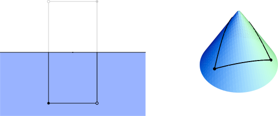
Figure 1: Straight lines between two points on ${\mathbb{C}}^{2}/{\mathbb{Z}}_{2}$.

The interpretation of these modes as bits of massive strings goes exactly as in the undeformed case [4]. According to the AdS/CFT correspondence, in the limit of large ’t Hooft coupling $\lambda$, the system should be described in terms of classical gravity with some string probes on the background. In this regime, using normalized distances $r$, the energies of the non-BPS modes are order

$$E_{ab}^{\alpha\beta}\sim\lambda^{1/2}|r_{a}-r_{b}^{-\alpha,\alpha-\beta}|\,.$$ (35)

where we have used the radius normalization found in the previous section to rewrite the mass terms in terms of the ’t Hooft coupling, and unit vectors on the sphere $r_{a}$. At strong coupling, the distance between the points dominates the energy of the string bits. Finite small energy string bits (energy of order one) require very small $|r_{a}-r_{b}^{-\alpha,\alpha-\beta}|$ and the segments between $r_{a}$ and $r_{b}^{-\alpha,\alpha-\beta}$ become tangent to the 5-sphere. These segments have to be joined into closed loops because we need to make a gauge invariant state.

We can consider these small segments as short bits of strings localized on the geometrical $S^{5}/{\mathbb{Z}}_{n}\times{\mathbb{Z}}_{n}$. In the case of strings on $AdS_{5}\times S^{5}$, it was shown in [6] that this description in terms of free short string bits was useful for the BMN limit, but longer string bits should be treated as interacting fields. Even though long string bits are interacting, the leading order perturbative evaluation of their energies gives the correct order of magnitude estimates for string energies and one can also use them to get some intuition on the eigenvalue geometry they are associated with.

4 Energy for BMN states

In this section we repeat a similar analysis to that of [6] to obtain an all-loop expression for the BMN operators energy in the $q$-deformed theory. To do that, we compute the approximate energy of the state resulting when we excite the ground state (17) with a BMN or BMN-like operator. BMN operators in marginal deformations of ${\cal N}=4$ SYM have been already studied in the literature [23, 24, 25], by considering appropriate deformations of the usual spin chain describing the dilatation operator. For instance, consider the dilatation operator in the two spin sector, at the 1-loop approximation, and with a deformation parameter $q=r\exp(2\pi i\beta)$. For a real deformation $q=r$, the dilatation operator turns out to be a periodic XXZ spin chain [23, 24]. The anisotropy parameter is a function of the deformation parameter such that $\Delta(r)\leq 1$ and then the spin chain is always ferromagnetic. When the deformation parameter presents a non-trivial phase, it is possible to perform a position dependent change of basis. In this particular new basis the Hamiltonian of an XXZ spin chain is recovered and the phase of the deformation is totally encoded in some twisted boundary conditions and a deformation in the cyclicity condition [24]. Moreover, in the case we are interested in, i.e. when the deformation parameter is a pure phase $q=\exp(2\pi i\beta)$, the chain becomes an XXX spin chain with twisted boundary conditions. The twisting factor is $q^{J}$ where $J$ is the length of the spin chain.

It turns out that BMN-like operators with two different holomorphic impurities are essentially identical to those of the undeformed theory [25] and the momentum numbers in the 1-loop energy are shifted $k/J\to k/J\pm\beta$. A consistent BMN limit for this spin chain requires that $k\pm\beta J$ should be kept finite in the $J\to\infty$ limit. In our case, it means that $k\pm J/n$ should be finite. So, we will consider the following BMN-like operator for exciting the ground state (17),

$$O_{k}\sim\sum_{l=0}^{J}\exp(i\varphi l){\rm tr}(Z^{l}XZ^{J-l}Y)\;,$$ (36)

where $\varphi$ is the usual BMN phase $\varphi=\frac{2\pi k}{J}$. We take $Z$ to be of the form (11) and the corresponding eigenvalues $\lambda^{3}_{a}$ given by the distribution obtained in section 3. On the other hand, fields $Y$ and $X$ include non-BPS modes, that can be treated as creation operators in a quantum system like (33). We will refer to them as $\lambda^{\!1\ \alpha\beta\dagger}_{ab}$ and $\lambda^{\!2\ \alpha\beta\dagger}_{ab}$. They satisfy the usual creation-annihilation algebra

$$[\lambda^{\alpha\beta}_{ab},\lambda^{\gamma\delta\dagger}_{cd}]=\delta_{ad}\delta_{bc}\delta^{\alpha\gamma}\delta^{\beta\delta}\,.$$ (37)

The above operator is represented by the following state

$$|\psi_{k}\rangle\sim\sum_{l=0}^{J}e^{i\varphi l}\sum_{\alpha,\beta}\sum_{a,b}q^{l(\alpha-\beta+1)+(\alpha+1)(\beta-s)}(\lambda^{3}_{a})^{l}(\lambda^{3}_{b})^{J-l}\lambda^{\!2\ \alpha\beta\dagger}_{ab}\lambda^{\!1\ s-\alpha-1,s-\beta-1\dagger}_{ba}\hat{\psi}_{0}{|0\rangle}\;.$$ (38)

The integer $s$ is the reduction modulo $n$ of the number of sites $J$. We have written the wave function $\hat{\psi}_{0}$ in the coordinate basis and the non-BPS modes as creation operators acting on the vacuum ${|0\rangle}$ of non-BPS modes.

We compute the energy of the above state, as an expectation value,

$$E\sim\frac{\langle\psi_{k}|H^{total}|\psi_{k}\rangle}{\langle\psi_{k}|\psi_{k}\rangle}\;.$$ (39)

The Hamiltonian (33) tells us that the oscillators carry an energy

$$E^{\alpha,\beta}_{ab}=\omega_{ab}^{1,\alpha\beta}+\omega_{ba}^{2,r-\alpha-1,r-\beta-1}\;.$$ (40)

Including the energy of the diagonal piece the total energy is

$$E^{total}=J+\langle E^{osc}\rangle\;.$$ (41)

Then, we have to compute the average energy of the oscillators (40) for the wave function (38). This results in the following integral

$$\langle E^{osc}\rangle=\frac{\int\prod dx^{c}|\hat{\psi}_{0}|^{2}\sum_{a,b,\alpha,\beta}|\sum_{l}e^{il\varphi}q^{l(\alpha-\beta+1)}(\lambda^{3}_{a})^{l}(\lambda^{3}_{b})^{J-l}|^{2}\left(\omega_{ab}^{1,\alpha\beta}+\omega_{ba}^{2,r-\alpha-1,r-\beta-1}\right)}{\int\prod dx^{c}|\hat{\psi}_{0}|^{2}\sum_{a,b,\alpha,\beta}|\sum_{l}e^{il\varphi}q^{l(\alpha-\beta+1)}(\lambda^{3}_{a})^{l}(\lambda^{3}_{b})^{J-l}|^{2}}$$ (42)

As it was done in the undeformed case [6], we can compute this average by a saddle point approximation. The first thing to notice is that both integral, in the denominator and in the numerator are dominated by the configurations that maximize $|\psi_{0}|^{2}$. This means that $\vec{\lambda}_{a}$ and $\vec{\lambda}_{b}$ should be located exactly on the orbifolded sphere $\tilde{\Omega}_{5}={S}^{5}/{\mathbb{Z}}_{n}\times{\mathbb{Z}}_{n}$. More precisely, in the thermodynamic limit sums $\sum_{a}$ are converted into integrals over the complex orbifold ${\mathbb{C}}^{3}/{\mathbb{Z}}_{n}\times{\mathbb{Z}}_{n}$ which, using the distribution $\rho_{0}(x)$, are reduced to integrals over $\tilde{\Omega}_{5}$.

$$\langle E^{osc}\rangle\simeq\frac{\int d\tilde{\Omega}_{5}d{\tilde{\Omega}^{\prime}}_{5}\sum_{\alpha,\beta}|\sum_{l}e^{il\varphi}q^{l(\alpha-\beta+1)}(\lambda^{3})^{l}({\lambda^{3}}^{\prime})^{J-l}|^{2}\left(\omega_{(\lambda\lambda^{\prime})}^{2,\alpha\beta}+\omega_{(\lambda^{\prime}\lambda)}^{1,r-\alpha-1,r-\beta-1}\right)}{\int d\tilde{\Omega}_{5}d{\tilde{\Omega}^{\prime}}_{5}\sum_{\alpha,\beta}|\sum_{l}e^{il\varphi}q^{l(\alpha-\beta+1)}(\lambda^{3})^{l}({\lambda^{3}}^{\prime})^{J-l}|^{2}}$$ (43)

Using $\lambda^{3}=r_{0}\cos\theta\exp(i\phi)$, the square of the sum can be rephrased as

$$\left|\sum_{l}e^{il\varphi}q^{l(\alpha-\beta-1)}(\lambda^{3})^{l}({\lambda^{3}}^{\prime})^{J-l}\right|^{2} = r_{0}^{2J}\sum_{l}\sum_{l^{\prime}}(\cos\theta)^{l+l^{\prime}}(\cos\theta^{\prime})^{2J-l-l^{\prime}}\times$$

$$~{}~{}~{}\exp\left[i(l-l^{\prime})\left(\varphi+\phi-\phi^{\prime}+\frac{2\pi}{n}(\alpha-\beta+1)\right)\right]$$

The BMN limit requires $J\to\infty$. This serves for improving the saddle point approximation thanks to the extra powers of $\cos\theta$ and $\cos\theta^{\prime}$ in the angular integrals. They are maximized when $|\lambda^{3}|$ and $|{\lambda^{3}}^{\prime}|$ take their maximum value on $\tilde{\Omega}_{5}$, i.e. when $\cos\theta=\cos\theta^{\prime}=1$. This corresponds to a geometrical localization for the string with large angular momentum $J$ around a null geodesic. Because of this localization the distances in the frequencies of the non-BPS modes are simplified. For instance,

$$|\vec{x}-\vec{x^{\prime}}^{-\alpha,\alpha-\beta}|^{2}~{}\to~{}|\lambda^{3}-q^{\beta-\alpha}{\lambda^{3}}^{\prime}|^{2}=4r_{0}^{2}\sin^{2}\left(\frac{1}{2}\left(\phi-\phi^{\prime}+{2\pi}(\alpha-\beta)/n\right)\right)\,.$$ (45)

A similar simplification takes place for the other frequency, leading to the same value (45). Moreover, in the large $J$ limit, we can approximate the sum over relative phases in (4) by a delta function and compute easily the remaining angular integrals. The result is that the amount $\phi-\phi^{\prime}+{2\pi}(\alpha-\beta)/n$ is sharply peaked at the value $\varphi+2\pi/n$, and the energy of the oscillators is

$$\langle E^{osc}\rangle=2\sqrt{1+\frac{2g^{2}_{YM}r_{0}^{2}}{n\pi^{2}}\sin^{2}\left(\frac{\varphi+2\pi/n}{2}\right)}\;,$$ (46)

Using the value we obtained $r_{0}=\sqrt{\frac{mn^{2}}{2}}$ in the section 3., $\varphi=\frac{2\pi k}{J}$ and taking the large $J$ limit, the energy for the oscillators reduces to

$$\langle E^{osc}\rangle=2\sqrt{1+g^{2}_{YM}N\left(\frac{k}{J}+\frac{1}{n}\right)^{2}}\;.$$ (47)

which is exactly the energy of BMN string excitations, with the appropriate normalization $g_{YM}^{2}=4\pi g_{s}$. From the gauge theory side it corresponds to an all orders result in perturbation theory. This all loop gauge theory result has been already reported in [21]. To obtain this result the authors of [21], extended the arguments used in [22] for the undeformed case. This includes using the equations of motion, but it is not clear if contact terms could spoil the use of these relations. Also, string states in the Lunin-Maldacena background have been considered by many authors [25, 26, 27, 28, 29]

We can also study in the same approximation BMN like states that are not reduced to the BMN limit. For example, we can consider the operator ${\rm tr}(Z^{J}Y)$. These operators have also been considered in [30, 31] (our results agree with those calculations). It is easy to see that this trace is zero on BPS states. In this case, we interpret $Y$ as the off-diagonal mode. Doing the same analysis as above, we also localize on the circle where $|z|=1$, and it turns out that the angle between the two eigenvalues that $Y$ connects is exactly given by the argument of $q$. This means that in the covering space, the mode $Y$ goes between an eigenvalue of $\Lambda_{Z}$ and a particular one of it’s images. At first sight one might think that one is violating the Gauss’ law for the corresponding state, because it seems as if the string state is an open string. However, this is a non-trivial loop in the orbifold geometry, so the correct interpretation is that the associated closed string state is actually in the twisted sector of the orbifold. This is exactly as should be. Twisted states of an abelian orbifold have non-trivial quantum symmetry quantum numbers. These discrete quantum numbers of the states can be calculated counting powers of $X,Y,Z$ modulo $n$ [13, 14]. It is easy to see that these jump assignments between images are all consistent with the quantum symmetry quantum numbers of states in these papers. Moreover, we can ask now under what conditions do some of these states survive in the BMN limit. It’s easy to show that if we take the BMN limit along $Z$, we need the state to be built only of small bits, and that forces us to have $\#Y-\#X=0\mod(n)$. This reproduces the BMN set of states of the orbifold ${\mathbb{C}}^{2}/{\mathbb{Z}}_{n}$, exactly as one would have expected from spin chain model considerations [24].

5 Discussion

In this paper we studied BPS configurations in some marginal deformations of SYM preserving ${\cal N}=1$ supersymmetry. We focused our attention to the case in which the commutator in the superpotential is deformed to a $q$-commutator, with $q$ being an $n$-th root of unity. In those cases, the gauge theory is dual to the near horizon geometry of $N$ D-branes in the complex orbifold ${\mathbb{C}}^{3}/{\mathbb{Z}}_{n}\times{\mathbb{Z}}_{n}$. The moduli space is described in terms of quantum mechanical $q$-commuting matrices. In the large $N$ limit, this is reduced to the study of density distributions of particles (interacting bosons) in a 6-dimensional phase space, that results from studying the moduli space of vacua of D-branes in the bulk. The ground state corresponds to a spherical distribution of bosons in ${\mathbb{C}}^{3}/{\mathbb{Z}}_{n}\times{\mathbb{Z}}_{n}$ and we identified this distribution as the compact factor of the dual geometry. Moreover, we considered non-BPS configurations by turning on non-trivial $q$-commutators. We argued that, as in the undeformed pure ${\cal N}=4$ SYM case, the energy of non-BPS modes is localized in this density distribution identified with the compact factor of the geometry, and they are considered as bits of massive strings. Thus, one of the accomplishment of this paper is that we have an explicit example of the extension of qualitative picture [4] for the appearance of spacetime geometry and locality in the strong ’t Hooft coupling regime beyond the standard $AdS_{5}\times S^{5}$/${\cal N}=4$ SYM.

Then, we proceeded as in [6] to compute the BMN energies to all orders in perturbation theory. The agreement with the string theory computation is complete where it is expected. This computation shows that the geometrical interpretation of the density distribution of boson is not just a qualitative picture, but that it can be used to reproduce concrete string theory calculations. We want to emphasize that the approximations we made are good only in the strict BMN limit. If we were interested in near-BMN corrections, we would have to deal with string bits of finite length and their interactions. The energies of these string states are analytic functions of the phase of $q$ (for $q$ unitary), so we can extend them to non-rational values of $q$ and we get agreement with other calculation of the corresponding energies.

Moreover, we have seen that the geometric picture given by this distribution of eigenvalues accounts correctly for discrete quantum numbers of string states, related to being in the twisted sector of the orbifold. This is a necessary step to claim that we understand the origin of geometry in a string theory setup that is not just supergravity.

Obviously, since we have succeeded in showing that for certain orbifolds of ${\cal N}=4$ SYM theory we are able to find the correct non-spherical horizon of the geometry, it is easy to conjecture that it will work the same way for all such supersymmetric orbifolds. Some recent progress in the better understanding of the structure of the field theory at orbifolds has been made recently in [32, 33] It would be interesting to show that this procedure works for other cases as well, such as the field theory obtained by placing D3-branes at a conifold singularity [34]. There is some preliminary evidence that this is possible in a large class of examples [35].

References

- [1] J. M. Maldacena, “The large N limit of superconformal field theories and supergravity,” Adv. Theor. Math. Phys. 2, 231 (1998) [Int. J. Theor. Phys. 38, 1113 (1999)] [arXiv:hep-th/9711200].
- [2] D. Berenstein, “A toy model for the AdS/CFT correspondence,” JHEP 0407, 018 (2004) [arXiv:hep-th/0403110].
- [3] H. Lin, O. Lunin and J. Maldacena, ‘Bubbling AdS space and 1/2 BPS geometries,” JHEP 0410, 025 (2004) [arXiv:hep-th/0409174].
- [4] D. Berenstein, “Large N BPS states and emergent quantum gravity,” arXiv:hep-th/0507203.
- [5] D. Berenstein, J. M. Maldacena and H. Nastase, “Strings in flat space and pp waves from N = 4 super Yang Mills,” JHEP 0204, 013 (2002) [arXiv:hep-th/0202021].
- [6] D. Berenstein, D. H. Correa and S. E. Vazquez, “All loop BMN state energies from matrices,” arXiv:hep-th/0509015.
- [7] D. Berenstein and R. G. Leigh, “Resolution of stringy singularities by non-commutative algebras,” JHEP 0106, 030 (2001) [arXiv:hep-th/0105229]. D. Berenstein, “Reverse geometric engineering of singularities,” JHEP 0204, 052 (2002) [arXiv:hep-th/0201093].
- [8] S. Kachru and E. Silverstein, “4d conformal theories and strings on orbifolds,” Phys. Rev. Lett. 80, 4855 (1998) [arXiv:hep-th/9802183].
- [9] R. G. Leigh and M. J. Strassler, “Exactly marginal operators and duality in four-dimensional N=1 supersymmetric gauge theory,” Nucl. Phys. B 447, 95 (1995) [arXiv:hep-th/9503121].
- [10] O. Lunin and J. Maldacena, “Deforming field theories with U(1) x U(1) global symmetry and their gravity duals,” JHEP 0505, 033 (2005) [arXiv:hep-th/0502086].
- [11] M. R. Douglas, “D-branes and discrete torsion,” arXiv:hep-th/9807235.
- [12] M. R. Douglas and B. Fiol, “D-branes and discrete torsion. II,” JHEP 0509, 053 (2005) [arXiv:hep-th/9903031].
- [13] D. Berenstein and R. G. Leigh, “Discrete torsion, AdS/CFT and duality,” JHEP 0001, 038 (2000) [arXiv:hep-th/0001055].
- [14] D. Berenstein, V. Jejjala and R. G. Leigh, “Marginal and relevant deformations of N = 4 field theories and non-commutative moduli spaces of vacua,” Nucl. Phys. B 589, 196 (2000) [arXiv:hep-th/0005087].
- [15] N. Dorey, T. J. Hollowood and S. P. Kumar, “S-duality of the Leigh-Strassler deformation via matrix models,” JHEP 0212, 003 (2002) [arXiv:hep-th/0210239].
- [16] N. Dorey, “S-duality, deconstruction and confinement for a marginal deformation of N = 4 SUSY Yang-Mills,” JHEP 0408, 043 (2004) [arXiv:hep-th/0310117].
- [17] G. Bertoldi and N. Dorey, “Non-critical superstrings from four-dimensional gauge theory,” arXiv:hep-th/0507075.
- [18] C. h. Ahn and J. F. Vazquez-Poritz, “Deformations of flows from type IIB supergravity,” arXiv:hep-th/0508075.
- [19] R. Hernandez, K. Sfetsos and D. Zoakos, “Gravity duals for the Coulomb branch of marginally deformed N = 4 Yang-Mills,” arXiv:hep-th/0510132.
- [20] J. P. Rodrigues, “Large N Spectrum of two Matrices in a Harmonic Potential and BMN energies,” arXiv:hep-th/0510244.
- [21] V. Niarchos and N. Prezas, “BMN operators for N = 1 superconformal Yang-Mills theories and associated string backgrounds,” JHEP 0306, 015 (2003) [arXiv:hep-th/0212111].
- [22] A. Santambrogio and D. Zanon, “Exact anomalous dimensions of N = 4 Yang-Mills operators with large R charge,” Phys. Lett. B 545, 425 (2002) [arXiv:hep-th/0206079].
- [23] R. Roiban, “On spin chains and field theories,” JHEP 0409, 023 (2004) [arXiv:hep-th/0312218].
- [24] D. Berenstein and S. A. Cherkis, “Deformations of N = 4 SYM and integrable spin chain models,” Nucl. Phys. B 702, 49 (2004) [arXiv:hep-th/0405215].
- [25] S. A. Frolov, R. Roiban and A. A. Tseytlin, “Gauge - string duality for superconformal deformations of N = 4 super Yang-Mills theory,” arXiv:hep-th/0503192.
- [26] S. Frolov, “Lax pair for strings in Lunin-Maldacena background,” JHEP 0505, 069 (2005) [arXiv:hep-th/0503201].
- [27] N. Beisert and R. Roiban, “Beauty and the twist: The Bethe ansatz for twisted N = 4 SYM,” JHEP 0508, 039 (2005) [arXiv:hep-th/0505187].
- [28] R. de Mello Koch, J. Murugan, J. Smolic and M. Smolic, “Deformed PP-waves from the Lunin-Maldacena background,” JHEP 0508, 072 (2005) [arXiv:hep-th/0505227].
- [29] T. Mateos, “Marginal deformation of N = 4 SYM and Penrose limits with continuum spectrum,” JHEP 0508, 026 (2005) [arXiv:hep-th/0505243].
- [30] S. Penati, A. Santambrogio and D. Zanon, “Two-point correlators in the beta-deformed N = 4 SYM at the next-to-leading order,” JHEP 0510, 023 (2005) [arXiv:hep-th/0506150].
- [31] A. Mauri, S. Penati, A. Santambrogio and D. Zanon, “Exact results in planar N = 1 superconformal Yang-Mills theory,” arXiv:hep-th/0507282.
- [32] N. Beisert and R. Roiban, “The Bethe ansatz for Z(S) orbifolds of N = 4 super Yang-Mills theory,” arXiv:hep-th/0510209.
- [33] D. Sadri and M. M. Sheikh-Jabbari, “Integrable spin chains on the conformal moose,” arXiv:hep-th/0510189.
- [34] I. R. Klebanov and E. Witten, “Superconformal field theory on threebranes at a Calabi-Yau singularity,” Nucl. Phys. B 536, 199 (1998) [arXiv:hep-th/9807080].
- [35] D. Berenstein and R. Corrado, work in progress.