February 2006

OCHA-PP-256   

hep-th/0511085

^† Department of Mathematics, Faculty of Science and Technology, Keio University
3-14-1 Hiyoshi, Kohoku-ku, Yokohama 223-8522, Japan
 
^§ Department of Physics, Faculty of Engineering, Musashi Institute of Technology
1-28-1 Tamazutsumi, Setagaya-ku, Tokyo 158-8557, Japan
^∗ Department of Physics, Faculty of Science, Ochanomizu University
2-1-1 Otsuka, Bunkyo-ku, Tokyo 112-8610, Japan
  ^† sako@math.keio.ac.jp
                 ^∗ tsuzuki@phys.ocha.ac.jp

Dimensional Reduction of Seiberg-Witten Monopole Equations, ${\cal N}=2$ Noncommutative Supersymmetric Field Theories and Young Diagrams

Akifumi Sako^†  ,  Toshiya Suzuki${}^{\S}{}^{\ast}$

1 Introduction

The Seiberg-Witten theory causes a revolution of nonperturbative analysis for ${\cal N}=2$ supersymmetric Yang-Mills theories [1, 2]. In the Seiberg-Witten theory, the instanton effects of ${\cal N}=2$ supersymmetric Yang-Mills theories are encoded in the pre-potential, which is defined by using the Seiberg-Witten curve. (See, for example, [3] and references there in.) The Seiberg-Witten theory also provides a powerful tool, the monopole equation, to investigate the topology of $4$ dimensional manifolds [4, 5]. The monopole equations are more tractable than the instanton equation, and yield many results in mathematics as well as physics.

Meanwhile, instanton calculus has developed by using ADHM data or D-instanton. (See, for example, [6].) Particularly, an important calculation technology for ${\cal N}=2$ supersymmetric Yang-Mills theories is brought by Nekrasov [7]. After [7], many related works have been made [8]-[38]. In [7] and so on, the localization theorem plays an essential role [39]-[42]. (See also [43, 44].) The localization theorem is valid when the theory has symmetries which correspond to some group action and the group action has isolated fixed points. It is expected that many kinds of calculations of ${\cal N}>1$ supersymmetric gauge theory are carried out by using this theorem.

It is shown that partition functions of ${\cal N}>1$ supersymmetric gauge theories on noncommutative (N.C.) ${\mathbb{R}}^{2D}$ are invariant under the N.C. parameter change [45]. Therefore we can perform the calculation at the large N.C. parameter limit. As discussed in [45]-[48], taking this limit causes dimensional reduction, and we can calculate the partition functions by using the theory after dimensional reduction. For this reason, it is important to investigate the dimensional reduction.

In this article, we will study a $0$ dimensional model given by dimensional reduction of Seiberg-Witten monopole equations derived from ${\cal N}=2$ supersymmetric $U(1)$ theory on N.C. ${\mathbb{R}}^{4}$. The equations are equivalent to the ADHM equations and the Dirac equation reduced to $0$ dimension. The equations are also equivalent to the dimensional reduction of non-Abelian $U(N)$ Seiberg-Witten monopole equations on commutative ${\mathbb{R}}^{4}$ at the large $N$ limit. In this paper, we investigate both cases of finite $N$ and infinite $N$. The finite $N$ case is not only the toy model, but also the model that is possible to be implanted into the $N=\infty$ theory and the results are valid for some special cases of $N=\infty$ model. We will find that the solutions of the equations are also interpreted as a configuration of brane anti-brane system. The theory has global symmetries under torus actions originated in space rotations and gauge symmetries. The torus actions define their fixed point equations. We will investigate the fixed point equations and the dimensional reduction of the Seiberg-Witten monopole equations. We will show that the Dirac equation is trivial when the fixed point equations and the ADHM equations are satisfied. For finite $N$ case, it is known that solutions satisfying the fixed point equations and the ADHM equations are isolated and classified by the Young diagrams [49]. We will give a new proof of this statement by solving the ADHM equations and the fixed point equations concretely and by giving graphical interpretation of the field components and these equations.

Here is the organization of this article. In section 2, we review the ${\cal N}=2$ supersymmetric gauge theory on ${\mathbb{R}}^{4}$ and N.C. ${\mathbb{R}}^{4}$ with a hypermultiplet. In section 3, a D-brane interpretation is discussed. In section4, we deform the BRS transformation by using the global symmetries of the theory. In section 5, we solve the Seiberg-Witten monopole equations reduced to $0$ dimension and the fixed point equations, and show our main claims. In section 6, we briefly comment on the localization theorem. Section 7 is summary of this article.

2 ${\cal N}=2$ Supersymmetric $U(1)$ Theory on N.C. ${\mathbb{R}}^{4}$

In this section we review ${\cal N}=2$ supersymmetric theory and its topological twist on ${\mathbb{R}}^{4}$ and N.C. ${\mathbb{R}}^{4}$. We consider the case with hypermultiplet [50]-[54]. For conventions in this article, see appendix A.

At first, we set up the model of the ${\cal N}=2$ supersymmetric theory on ${\mathbb{R}}^{4}$. $SO(4)$ spacetime rotation of $4$ dimensional Euclidean space is locally equivalent to $SU(2)_{L}\otimes SU(2)_{R}$. ${\cal N}=2$ supersymmetric theories have $SU(2)_{I}$ R-Symmetry. The supersymmetry generators $Q_{\alpha i}$, $\bar{Q}_{\dot{\alpha}i}$ have indices $i=1,2$ for the R-symmetry. ${\cal N}=2$ supersymmetric theories on ${\mathbb{R}}^{4}$ have following symmetry;

$$H=SU(2)_{L}\otimes SU(2)_{R}\otimes SU(2)_{I}\ .$$ (1)

The supersymmetric gauge multiplet is given by

$$\begin{array}[]{ccc}&A_{\mu}&{}\hfil\\ \psi^{1}&\phantom{\psi^{q}}&\psi^{2}\ \ .\\ &\phi&{}\hfil\end{array}$$ (5)

Here $\psi^{1}$,$\psi^{2}$ and $\bar{\psi}^{1}$,$\bar{\psi}^{2}$ are Weyl spinors and their CPT conjugate. $\phi$ and $\bar{\phi}$ are scalar fields. Their quantum number of $H$ are assigned as

$$\begin{array}[]{ccc}\psi^{1}=(1/2,0,1/2),&\psi^{2}=(1/2,0,1/2),&\phi=(0,0,0),\\ \bar{\psi}^{1}=(0,1/2,1/2),&\bar{\psi}^{2}=(0,1/2,1/2),&\bar{\phi}=(0,0,0).\end{array}$$ (8)

The action functional is given by

$$L= -\frac{1}{4}F_{\mu\nu}^{a}F^{\mu\nu}_{a}-i\bar{\psi}_{\dot{\alpha}i}^{a}\bar{\sigma}^{\mu\dot{\alpha}\alpha}D_{\mu}\psi_{\alpha a}{}^{i}-D_{\mu}\bar{\phi}^{a}D^{\mu}\phi_{a}$$ (9)

$$-\frac{i}{\sqrt{2}}\psi^{\alpha ia}[\bar{\phi},\psi_{\alpha i}]_{a}-\frac{i}{\sqrt{2}}\bar{\psi}_{\dot{\alpha}}{}^{ia}[\phi,\bar{\psi}^{\dot{\alpha}}{}_{i}]_{a}-\frac{1}{2}[\bar{\phi},\phi]^{2},\ .$$ (10)

The supersymmetric transformation with parameter $\xi$ and ${\bar{\xi}}$ are written as

$$\delta A_{\mu} = i\xi^{\alpha i}\sigma_{\mu\alpha\dot{\alpha}}\bar{\psi}^{\dot{\alpha}}{}_{i}-i\psi^{\alpha i}\sigma_{\mu\alpha\dot{\alpha}}\bar{\xi}^{\dot{\alpha}}{}_{i},$$

$$\delta\psi_{\alpha}{}^{i} = \sigma^{\mu\nu\,\beta}_{\,\,\alpha}\xi_{\beta}{}^{i}F_{\mu\nu}+\sqrt{2}i\sigma^{\mu}_{\alpha\dot{\alpha}}D_{\mu}\phi\bar{\xi}^{\dot{\alpha}i}+[\phi,\bar{\phi}]\xi_{\alpha}{}^{i},$$

$$\delta\bar{\psi}_{\dot{\alpha}i} = -\bar{\xi}_{\dot{\beta}i}\bar{\sigma}^{\mu\nu\dot{\beta}}_{\quad\,\dot{\alpha}}F_{\mu\nu}+\sqrt{2}i\xi^{\alpha i}\sigma^{\mu}_{\alpha\dot{\alpha}}D_{\mu}\bar{\phi}-[\phi,\bar{\phi}]\bar{\xi}_{\dot{\alpha}i},$$

$$\delta\phi = \sqrt{2}\xi^{\alpha i}\psi_{\alpha i},$$

$$\delta\bar{\phi} = \sqrt{2}\bar{\xi}^{\dot{\alpha}}_{i}\bar{\psi}_{\dot{\alpha}}{}^{i}.$$ (11)

To classify the solutions of BPS equations by equivariant cohomology, let us introduce topological twist here [55, 56]. We use a diagonal subgroup $SU(2)_{R^{\prime}}$ in $SU(2)_{R}\otimes SU(2)_{I}$ of $H$. We redefine the spacetime rotation group by

$$K^{\prime}:=SU(2)_{L}\otimes SU(2)_{R^{\prime}},$$ (12)

Then combinations of spinors whose quantum number of $H$ are $(1/2,0,1/2)\oplus(0,1/2,1/2)$ have quantum number $(1/2,1/2)\oplus(0,1)\oplus(0,0)$ of $K^{\prime}$. Particularly $(0,0)$ is scalar and $Q=\epsilon^{\dot{\alpha}i}\bar{Q}_{\dot{\alpha}i}$ is a BRS operator. Fermionic fields are similarly topological twisted as $\psi^{i}\ (\frac{1}{2},0,\frac{1}{2})\rightarrow\psi_{\mu}\ (\frac{1}{2},\frac{1}{2})\$ and $\bar{\psi}^{i}\ (0,\frac{1}{2},\frac{1}{2})\rightarrow\chi_{\mu\nu}\ (0,1)\ \oplus\ \eta\ (0,0)$. BRS transformations are given as

$${\hat{\delta}}A_{\mu} =i\psi_{\mu},\ \ \ \ \ {\hat{\delta}}\psi_{\mu} =-D_{\mu}\phi,\ \ \ \ \ {\hat{\delta}}\phi=0,$$

$${\hat{\delta}}\chi_{\mu\nu} =H_{\mu\nu},\ \ \ \ \ {\hat{\delta}}\bar{\phi} =i\eta,$$

$${\hat{\delta}}H_{\mu\nu} =i[\phi,\chi_{\mu\nu}],\ \ \ \ \ {\hat{\delta}}\eta =[\phi,\bar{\phi}]\ .$$ (13)

Here we introduce auxiliary field $H_{\mu\nu}$.

Next step, let us introduce hypermultiplets. ${\cal N}=2$ hypermultiplet consists from two Weyl fermions $\lambda_{\!q}$ and $\lambda_{\!\tilde{q}}^{\dagger}$ and two complex scalar boson ; $q$ and $\tilde{q}^{\dagger}$

$$\lambda_{q}$$

$$q\quad {\tilde{q}}^{\dagger}\ .$$

$${\lambda}_{\tilde{q}}^{\dagger}\quad$$

The definition of the symbol $\dagger$ is seen in appendix A. Their supersymmetric transformations are given by

$$\delta q^{i} = -\sqrt{2}\xi^{\alpha i}\lambda_{q\alpha}+\sqrt{2}\bar{\xi}_{\dot{\alpha}}{}^{i}\bar{\lambda}_{\tilde{q}}^{\dot{\alpha}},$$

$$\delta\lambda_{q\alpha} = -\sqrt{2}i\sigma^{\mu}_{\alpha\dot{\alpha}}D_{\mu}q^{i}\bar{\xi}^{\dot{\alpha}}{}_{i}-2T_{a}q^{i}\bar{\phi}^{a}\xi_{\alpha i},$$

$$\delta\bar{\lambda}_{\tilde{q}}^{\dot{\alpha}} = -\sqrt{2}i\bar{\sigma}^{\mu\dot{\alpha}\alpha}D_{\mu}q^{i}\xi_{\alpha i}+2T_{a}q^{i}\phi^{a}\bar{\xi}^{\dot{\alpha}}{}_{i},$$ (14)

where $T_{a}$ is a generator of gauge group. In the following, we consider the case that representation of the gauge group of the hypermultiplet is fundamental representation. After topological twisting, BRS transformations are given by

$${\hat{\delta}}q^{\dot{\alpha}} = {\psi}_{\!q}^{\dot{\alpha}},\ \ {\hat{\delta}}q_{\dot{\alpha}}^{\dagger}={\psi}^{\dagger}_{\!q\dot{\alpha}},$$

$${\hat{\delta}}{\psi}_{\!q}^{\dot{\alpha}} = -i\phi^{a}T_{a}q^{\dot{\alpha}},\ \ {\hat{\delta}}{\psi}^{\dagger}_{\!q\dot{\alpha}}=iq_{\dot{\alpha}}^{\dagger}\phi^{a}T_{a},$$

$${\hat{\delta}}\chi_{q\alpha} = H_{q\alpha},\ \ {\hat{\delta}}\chi^{{\dagger}\alpha}_{q}=H^{{\dagger}\alpha}_{q}$$

$${\hat{\delta}}H_{q\alpha} = -i\phi^{a}T_{a}\chi_{q\alpha},\ \ {\hat{\delta}}H^{{\dagger}\alpha}_{q}=i\chi^{{\dagger}\alpha}_{q}\phi^{a}T_{a},$$ (15)

where fields are rescaled and also auxiliary field $H_{q\alpha}$ is introduced. After topological twisting, we rename the fermions as $\lambda_{q}\rightarrow\chi_{q}$ and $\bar{\lambda}_{q}\rightarrow\psi_{q}$.

Using these field contents, let us construct the action of Seiberg-Witten theory. The action with fundamental hypermultiplet terms are defined by

$$S=k-\hat{\delta}\Psi$$ (16)

where $k$ is instanton number

$$k=\frac{1}{8\pi^{2}}\int{\hbox{\rm Tr}}(F_{A}\wedge F_{A}),$$ (17)

and $\Psi$ is a gauge fermion;

$$\Psi = -\chi^{\mu\nu a}_{+}\{H^{a}_{+\mu\nu}-s_{+\mu\nu}^{a}\}-\chi^{\dagger\alpha}_{q}\{H_{q\alpha}-s_{\alpha}\}-\{H^{\dagger\alpha}_{q}-s^{\dagger\alpha}\}\chi_{q\alpha}$$ (18)

$$+i[\phi,{\bar{\phi}}]^{a}\eta^{a}+D_{\mu}{\bar{\phi}}^{a}\psi^{\mu a}-(-iq^{\dagger}_{\dot{\alpha}}{\bar{\phi}})\psi^{\dot{\alpha}}_{q}-\psi^{\dagger}_{q\dot{\alpha}}(i{\bar{\phi}}q^{\dot{\alpha}})\ ,$$

Here

$$s^{\mu\nu}(A,q,q^{\dagger}) = F^{+\mu\nu}_{a}+q^{\dagger}\bar{\sigma}^{\mu\nu}T_{a}q.$$

$$s^{\alpha}(A,q) = \sigma^{\mu}D_{\mu}q=\ooalign{\hfil$/$\hfil\crcr$D$}q\ .$$ (21)

After integration of the auxiliary fields $H_{+\mu\nu}$ and $H_{q}$, the bosonic action are given as

$$S_{B} = \int\!d^{4}\!x\sqrt{g}\biggl{[}\frac{1}{4}|s^{\mu\nu}|^{2}+\frac{1}{2}|s^{\alpha}|^{2}\biggl{]}+\cdots\ .$$ (22)

Notice that when the gauge group is $U(1)$ and the theory is defined on simple type commutative manifolds we get the Seiberg-Witten invariants as the partition function of this model [4, 5, 50, 51]. From (22) we get the BPS equations,

$$s^{\mu\nu}(A,q,q^{\dagger})=0\ ,\ s^{\alpha}(A,q)=0\ ,$$ (23)

which is known as the non-Abelian Seiberg-Witten monopole equations.

In the following, we investigate some properties of ${\cal N}=2$ supersymmetric gauge theory on N.C. ${\mathbb{R}}^{4}$ whose noncommutativity is defined as

$$[x^{\mu},x^{\nu}]=i\theta^{\mu\nu}\ ,$$ (24)

where the $\theta^{\mu\nu}$ is an element of an antisymmetric matrix and called N.C. parameter. For simplicity, we take

$$(\theta^{\mu\nu})=\left(\begin{array}[]{cc|cc}0&\theta^{1}&0&0\\ -\theta^{1}&0&0&0\\ \hline\cr 0&0&0&\theta^{2}\\ 0&0&-\theta^{2}&0\end{array}\right)\ \ .$$ (29)

In the following, we only use operator formalisms to describe the N.C. field theory, therefore the fields are operators acting on the Hilbert space ${\cal H}$. Then differential operators $\partial_{\mu}$ are expressed by using commutation brackets $-i\theta^{-1}_{\mu\nu}[x^{\nu},\ *]\equiv[\hat{\partial}_{\mu},*]$ and $\int d^{2D}x$ is replaced with $det(\theta)^{1/2}Tr_{\cal H}$.

When we consider only the case of N.C. ${\mathbb{R}}^{4}$, field theories are expressed by the Fock space formalism. (See appendix in [45].) In the Fock space representation, fields are expressed as $A_{\mu}=\sum{A_{\mu}}^{n_{1}n_{2}}_{m_{1}m_{2}}|n_{1},n_{2}\rangle\langle m_{1},m_{2}|$ , $\psi_{\mu}=\sum{\psi_{\mu}}^{n_{1}n_{2}}_{m_{1}m_{2}}|n_{1},n_{2}\rangle\langle m_{1},m_{2}|$ , etc. Therefore, the above BRS transformations are expressed as

$$\hat{\delta}{A_{\mu}}^{n_{1}n_{2}}_{m_{1}m_{2}}={\psi_{\mu}}^{n_{1}n_{2}}_{m_{1}m_{2}}\ \ ,\ \ \hat{\delta}{\psi_{\mu}}^{n_{1}n_{2}}_{m_{1}m_{2}}=(D_{\mu}\phi)^{n_{1}n_{2}}_{m_{1}m_{2}}\ \ ,\ \ \cdots\ \ .$$ (30)

where the covariant derivative is defined by $D_{\mu}\ *:=[\hat{\partial}_{\mu}+iA_{\mu}\ ,\ *\ ]$ with $\hat{\partial}_{\mu}:=-i\theta^{-1}_{\mu\nu}x^{\nu}$. The action functional is given by

$$S = Tr_{\cal H}\ L(A_{\mu},\dots;\hat{\partial}_{z_{i}},\hat{\partial}_{\bar{z}_{i}})$$ (31)

$$= Tr_{\cal H}tr\hat{\delta}\Psi\ .$$

Let us change the dynamical variables as

$$A_{\mu}\rightarrow\frac{1}{\sqrt{\theta}}\tilde{A}_{\mu},\ \ \psi_{\mu}\rightarrow\frac{1}{\sqrt{\theta}}\tilde{\psi}_{\mu},\ \ \bar{\phi}\rightarrow\frac{1}{\theta}\tilde{\bar{\phi}},\ \ \eta\rightarrow\frac{1}{\theta}\tilde{\eta},\ \ q\rightarrow\frac{1}{\sqrt{\theta}}\tilde{q},\ \ q^{\dagger}\rightarrow\frac{1}{\sqrt{\theta}}\tilde{q}^{\dagger}$$

$$\chi_{\mu\nu}^{+}\rightarrow\frac{1}{\theta}\tilde{\chi}_{\mu\nu}^{+},\ \ H_{\mu\nu}^{+}\rightarrow\frac{1}{\theta}\tilde{H}_{\mu\nu}^{+},\ \ \phi\rightarrow\tilde{\phi}\ \ \psi_{q}\rightarrow\frac{1}{\sqrt{\theta}}\tilde{\psi_{q}},\ \ \psi^{\dagger}_{q}\rightarrow\frac{1}{\sqrt{\theta}}\tilde{\psi}^{\dagger}_{q},$$

$$\chi_{q}\rightarrow\frac{1}{{\theta}}\tilde{\chi_{q}},\ \ \chi_{q}^{\dagger}\rightarrow\frac{1}{{\theta}}\tilde{\chi_{q}}^{\dagger},\ \ H_{q}\rightarrow\frac{1}{\theta}\tilde{H}_{q},\ \ H_{q}^{\dagger}\rightarrow\frac{1}{\theta}\tilde{H}_{q}^{\dagger}.$$ (32)

Note that this changing does not cause nontrivial Jacobian from the path integral measure because of the BRS symmetry. Then, the action is rewritten as

$$S\rightarrow\frac{1}{\theta^{2}}\tilde{S}\ \ \ ,\ \ \ L(A_{\mu},\dots;\hat{\partial}_{z_{i}},\hat{\partial}_{\bar{z}_{i}})\rightarrow\frac{1}{\theta^{2}}L(\tilde{A}_{\mu},\dots;-a_{i}^{\dagger},a_{i})\ \ .$$ (33)

Here the action in LHS depends on $\theta$ because the derivative is given by $\partial_{z_{i}}=-\sqrt{\theta^{-1}}[a_{i}^{\dagger},\ ]$ and so on. In contrast, the action $\tilde{S}$ in RHS does not depend on $\theta$ because all $\theta$ parameters are factorized out. Using the BRS symmetry, it is proved that the partition function is invariant under the deformation of $\theta$, because $\delta_{\theta}Z=-2(\delta\theta)\theta^{-3}\langle\tilde{S}\rangle=0$. As discussed in [45], the partition function of this theory is possible to be determined by using a lower dimension theory that is given by dimensional reduction. Therefore, the investigation of the dimensional reduction of the theories is important.

The dimensional reduction of Seiberg-Witten monopole equations (21) are expressed as

$$P^{\mu\nu\rho\tau}_{+}[A_{\rho},A_{\tau}]+q\bar{\sigma}^{\mu\nu}q^{\dagger}=0\ ,$$ (34)

$$\sigma^{\mu}A_{\mu}q=0\ ,$$ (35)

where $P^{\mu\nu\rho\tau}_{+}$ is a selfdual projection operator. These expressions are valid for the dimensional reduction of the non-Abelian theory on commutative ${\mathbb{R}}^{4}$. Using $q_{+}:=(q_{\dot{1}}+q_{\dot{2}})/{\sqrt{2}}$ and $q_{-}:=(q_{\dot{1}}-q_{\dot{2}})/{\sqrt{2}}$, if we start from the $U(1)$ theory on N.C.${\mathbb{R}}^{4}$, the equation (34) is rewritten as ADHM equations :

$$[A_{z_{1}},A_{z_{1}}^{\dagger}]+[A_{z_{2}},A_{z_{2}}^{\dagger}]+q_{-}q_{-}^{*T}-q_{+}q_{+}^{*T} = 0\ ,$$

$${}[A_{z_{1}},A_{z_{2}}]+q_{-}q_{+}^{*T} = 0\ .$$ (36)

Note that these operators in (36) are expressed by infinite dimensional matrices and the ADHM equations correspond to the instanton of $U(N)$ gauge group with instanton number $N$ at the large $N$ limit. We consider the finite $N$ situation in the next section.

3 D-brane Interpretation

In this article, we study detail of the solution of (34) and (35). On the N.C. ${\mathbb{R}}^{4}$ the fields appearing in (34) and (35) is infinite dimensional matrix acting on Hilbert space. But the equations are important even if the dimension of the matrix is finite, because there is a corresponding physical model. In this section, we consider the correspondence between Seiberg-Witten monopole equations, D-brane picture and (34) (35) [57].

At first, we construct the physical model by using the similar manner of the article [57]. (See also [58]-[65].)

The generalized second order effective action of $N$ $D3$-brane $N$ $\bar{D}3$-brane system without topological terms are given by

$$\int tr\left\{\frac{1}{4}F_{\mu\nu}^{(N)}F^{(N){\mu\nu}}+\frac{1}{4}F_{\mu\nu}^{(\bar{N})}F^{(\bar{N}){\mu\nu}}+|D^{\mu}\phi|^{2}+\frac{1}{2}(\tau^{2}-\phi\bar{\phi})^{2}\right\}\ .$$ (37)

Here the $F_{\mu\nu}^{(N)}$ and $F_{\mu\nu}^{(\bar{N})}$ are the curvature of the $A^{(N)}$ and $A^{(\bar{N})}$ , respectively, where $A^{(N)}$ and $A^{(\bar{N})}$ correspond to open strings attached on $D3$-brane and $\bar{D}3$-brane. Up to topological terms, we can rewrite this action as

$$\int tr\left\{\frac{1}{4}F_{\mu\nu}^{(\bar{N})}F^{(\bar{N}){\mu\nu}}+\frac{1}{2}|F_{{z}^{1}\bar{z}^{1}}^{(N)}+F_{{z}^{2}\bar{z}^{2}}^{(N)}+(\phi\bar{\phi}-\tau^{2})|^{2}+8|F_{{z}^{1}{z}^{2}}|^{2}+2|D_{\bar{z}_{\bar{1}}}\phi|^{2}+2|D_{\bar{z}_{\bar{2}}}\phi|^{2}\right\}\ .$$ (38)

From this action, considering the case of $A_{\mu}^{(\bar{N})}=0$, stationary points are given by

$$F_{{z}^{1}\bar{z}^{1}}^{(N)}+F_{{z}^{2}\bar{z}^{2}}^{(N)}+q_{-}q_{-}^{*T} = \zeta\ \ ,$$ (39)

$$F_{{z}^{1}{z}^{2}}^{(N)} = 0\ \ ,$$ (40)

$$D_{\bar{z}^{1}}q_{-} = 0\ \ ,$$ (41)

$$D_{\bar{z}^{2}}q_{-} = 0\ ,$$ (42)

where we replace $\phi$ by $q_{-}$ and $\tau^{2}$ by $\zeta$. Then, this is the Seiberg-Witten monopole equations with $q_{+}=0$ condition and back ground constant field $\zeta$. (See also the next section.) This case corresponds to the $\zeta>0$ as we will see in section 5. Note that $q_{-}$ can be regarded as a complex scalar field when we consider ${\mathbb{R}}^{4}$ case.

The solution of (34),(35) of finite matrix model is realized as some $D3$-$\bar{D}3$ configuration.

4 Deformed BRS Transformation

In this section, we will investigate the symmetry of the dimension reduction of (31) to $0$ dimension, and deform the BRS symmetry as ${\cal G}\otimes T^{N+2}$ equivariant derivative, where ${\cal G}$ is the gauge transformation group of $U(N)$ and $T^{N+2}$ is the torus action, in order to derive the fixed point equations. Note that the $U(N)$ symmetry is caused from the $U(1)$ symmetry if we consider the N.C. theory. As explained in section 2, the action functional is defined by infinite dimensional matrices when we start from N.C. theories, then N.C.$U(1)$ gauge symmetry is expressed by $U(\infty)$ symmetry. For simplicity, in some discussions of this paper, we restrict our analysis to the finite dimensional, $N\times N$, matrix case. ( Only proof of the theorem 3 in section 5 and the calculations of the partition function of a toy model in section 6 are based on discussions of finite $N$.) All of the fields contents , $A_{\mu},q$, etc, are given by $N\times N$ matrices. Then the $U(\infty)$ symmetry is also truncated to $U(N)$. From the viewpoint of N.C.field theory, there might be another type of solutions which is not studied in this article, and the following analysis might not be completed. On the other hand, as discussed in the previous section, the finite $N\times N$ theory has a $D3$-${\bar{D}}3$ brane interpretation, then it has physical applications.

The path integral for cohomological field theories reduced to the integral over the moduli space of vacuum. In our case, the moduli space is defined by solutions of (34),(35). As demonstrated in [7], the localization theorem is a powerful tool for path integrals of cohomological field theories. The localization theorem is valid when a theory under consideration has symmetries under some group actions, and the group actions have isolated fixed points. (For the localization theorem, see also section 6.) Therefore, to investigate solutions of the fixed point equation is important. This is the main subject of this paper.

Adding to the $U(N)$ gauge symmetry and the Lorentz symmetry $SO(4)=SU(2)_{L}\otimes SU(2)_{R}$, the action reduced to $0$ dimension has the next extra unitary symmetry, denoted by ${\tilde{U}}(N)$,

$$\delta^{{\tilde{U}}(N)}q_{\dot{\alpha}}=iq_{\dot{\alpha}}b,$$ (43)

where $b$ is a generator of ${\tilde{U}}(N)$. Recall that $q$ and $q^{\dagger}$ are fundamental representation of the gauge group. The gauge transformation of $q$ is defined by left action of the $U(N)$. Notice that if we define the gauge transformation by using right action, we can define another gauge symmetry with the corresponding gauge field. We do not introduce this gauge field, then the symmetry appears only after the dimensional reduction. This is the origin of ${\tilde{U}}(N)$.

Now we use the Abelian subgroup $U(1)^{2}\otimes U(1)^{N}$ of $SO(4)\otimes{\tilde{U}}(N)$. That is, we consider the following symmetry of the action.

$$\delta^{U(1)^{2}\otimes U(1)^{N}}A_{z_{i}} = -i\epsilon_{i}A_{z_{i}},$$ (45)

$$\delta^{U(1)^{2}\otimes U(1)^{N}}q_{\dot{\alpha}} = +i{{M_{R}}_{\dot{\alpha}}}^{\dot{\beta}}q_{\dot{\beta}}+iq_{\dot{\alpha}}b,$$ (46)

where $b=\mbox{diag.}(b_{1},\cdots,b_{N})$ is a generator of an Abelian subgroup $U(1)^{N}$ of ${\tilde{U}}(N)$, and $\epsilon_{i}\ (i=1,2)$ is a generator of an Abelian subgroup $U(1)^{2}$ of $SO(4)$, defined by

$$\delta A_{\mu}={M_{\mu}}^{\nu}A_{\nu}\ \ \ ,\ \ \ {M_{\mu}}^{\nu}=\left(\begin{array}[]{cccc}0&-\epsilon_{1}&&\\ +\epsilon_{1}&0&&\\ &&0&-\epsilon_{2}\\ &&-\epsilon_{2}&0\end{array}\right).$$ (47)

Also ${{M_{R}}_{\dot{\alpha}}}^{\dot{\beta}}$ is the generator of $U(1)\subset SU(2)_{R}$,

$${{M_{R}}_{\dot{\alpha}}}^{\dot{\beta}}=\left(\begin{array}[]{cc}0&\epsilon_{+}\\ \epsilon_{+}&0\end{array}\right)\ \ \ ,\ \ \ \epsilon_{+}=\frac{\epsilon_{1}+\epsilon_{2}}{2}.$$ (48)

By using above $U(1)^{2}\otimes U(1)^{N}$, let us deform the BRS symmetry from $\hat{\delta}$ to $\tilde{\delta}$. We define the deformation by replacing $\hat{\delta}^{2}=\delta^{U(N)gauge}_{(-\phi)}$ to

$${\tilde{\delta}}^{2}=\delta^{U(N)gauge}_{(-\phi)}+\delta^{U(1)^{N}}_{(b)}+\delta^{U(1)^{2}}_{(\epsilon_{1},\epsilon_{2})}.$$ (49)

Here $\delta^{G}_{(\Delta)}$ is a gauge transformation operator with the group $G$ and the transformation parameter $\Delta$. Then, for $\psi_{z_{i}}$ and $\psi_{q{\dot{\alpha}}}$, the BRS transformation rules are given by,

$${\tilde{\delta}}^{2}A_{z_{i}} = {\tilde{\delta}}\psi_{z_{i}}=i[A_{z_{i}},\phi]-i\epsilon_{i}A_{z_{i}},$$ (50)

$${\tilde{\delta}}^{2}q_{\dot{\alpha}} = {\tilde{\delta}}\psi_{q{\dot{\alpha}}}=-i\phi q_{\dot{\alpha}}+{{M_{R}}_{\dot{\alpha}}}^{\dot{\beta}}q_{\dot{\beta}}+iq_{\dot{\alpha}}b,$$ (51)

$${\tilde{\delta}}^{2}q^{{\dagger}{\dot{\alpha}}} = {\tilde{\delta}}{\psi_{q}}^{{\dagger}\dot{\alpha}}=q^{{\dagger}{\dot{\alpha}}}i\phi-{{M_{R}}^{\dot{\alpha}}}_{\dot{\beta}}q^{{\dagger}{\dot{\beta}}}-ibq^{{\dagger}{\dot{\alpha}}}.$$ (52)

Now we list the equations, solutions of which we will investigate. Some of them are the equations of motion, often called BPS equations. They are the same as (34) or (36),(35). However we take some deformation of them, to remove singular solutions. We introduce a nonzero number $\zeta$, and take

$$i([A_{z_{1}},A_{{\bar{z}}_{1}}]+[A_{z_{2}},A_{{\bar{z}}_{2}}])+q({\bar{\sigma}}_{z_{1}{\bar{z}}_{1}}+{\bar{\sigma}}_{z_{2}{\bar{z}}_{2}})q^{{\dagger}}=i\zeta,$$ (53)

$$i[A_{z_{1}},A_{z_{2}}]+q{\bar{\sigma}}_{z_{1}z_{2}}q^{{\dagger}}=0,$$ (54)

$$(A_{z_{1}}\sigma^{z_{1}}+A_{{\bar{z}}_{1}}\sigma^{{\bar{z}}_{1}}+A_{z_{2}}\sigma^{z_{2}}+A_{{\bar{z}}_{2}}\sigma^{{\bar{z}}_{2}})q=0.$$ (55)

(53),(54) are realized by the redefinition of $s^{\mu\nu}(A,q,q^{\dagger})$

$$s^{\mu\nu}(A,q,q^{\dagger})\rightarrow F^{+\mu\nu}+q\bar{\sigma}^{\mu\nu}q^{\dagger}-\zeta^{+}_{\mu\nu},$$

$$\zeta_{z_{1}{\bar{z}_{1}}}+\zeta_{z_{2}{\bar{z}_{2}}}=i\zeta\ ,\ \zeta_{z_{1}z_{2}}=0.$$ (56)

This constant $\zeta$ is considered as a back ground field and we define its BRS transformation by $\tilde{\delta}\zeta=0$. Then, we find that all of the above discussions in previous sections are valid although we add this back ground field. For later use, we rewrite them into

$$[A_{z_{1}},A_{{\bar{z}}_{1}}]+[A_{z_{2}},A_{{\bar{z}}_{2}}]-(q_{\dot{2}}q_{\dot{1}}^{*T}+q_{\dot{1}}q_{\dot{2}}^{*T})=\zeta,$$ (57)

$$[A_{z_{1}},A_{z_{2}}]+\frac{1}{2}(q_{\dot{1}}q_{\dot{1}}^{*T}-q_{\dot{2}}q_{\dot{2}}^{*T})+\frac{1}{2}(q_{\dot{1}}q_{\dot{2}}^{*T}-q_{\dot{2}}q_{\dot{1}}^{*T})=0,$$ (58)

$$(A_{{\bar{z}}_{1}}-A_{z_{2}})q_{\dot{2}}-(A_{{\bar{z}}_{1}}+A_{z_{2}})q_{\dot{1}}=0,$$ (59)

$$(A_{{\bar{z}}_{2}}+A_{z_{1}})q_{\dot{2}}-(A_{{\bar{z}}_{2}}-A_{z_{1}})q_{\dot{1}}=0.$$ (60)

The rest of the equations to be investigated are the fixed point equations of the deformed BRS transformation (50) - (52). They are given by

$$i[A_{z_{i}},\phi]-i\epsilon_{i}A_{z_{i}}=0,$$ (61)

$$-i\phi q_{\dot{\alpha}}+{{M_{R}}_{\dot{\alpha}}}^{\dot{\beta}}q_{\dot{\beta}}+iq_{\dot{\alpha}}b=0.$$ (62)

In the next section, we will investigate solutions of (53),(54),(55),(61),(62), and will show that they have isolated solutions. This fact guarantees that the localization theorem is valid to our case.

5 Solutions of (53),(54),(55),(61),(62)

In this section, we solve (53),(54)(55),(61),(62), and show that these equations have only isolated solutions and the solutions are expressed by the Young diagrams. Notice that our analysis is also valid to a case where $q_{\alpha}$’s are $N\times k,(k\neq N)$ matrices, though we will treat $q_{\alpha}$ as $N\times N$ matrices in this section. If we take $q_{\dot{\alpha}}$ to be $N\times k$, $q_{\dot{\alpha}}^{*T}$ to be $k\times N$ and $b\in u(k)$, our proof in this section includes a new proof for Prop.5.6. in [49].

First of all, we diagonalize $\phi$ by using the $U(N)$ gauge symmetry,

$$\phi=\mbox{diag.}(\phi_{1},\phi_{2},\cdots,\phi_{N}).$$ (63)

Next we tackle (61) and (62). From (61) we see immediately that if and only if,

$$\phi_{J}-\phi_{I}=\epsilon_{i},$$ (64)

$A_{z_{i}\ IJ}$ could be non-zero,

$$A_{z_{i}\ IJ}\neq 0.$$ (65)

Also from (62) we see that if and only if,

$$\phi_{I}=b_{J}\pm\epsilon_{+},$$ (66)

$q_{\dot{1}\ IJ}$ and $q_{\dot{2}\ IJ}$ could be non-zero,

$$q_{\dot{1}\ IJ}=\pm q_{\dot{2}\ IJ}\neq 0.$$ (67)

Notice $q_{\dot{1}\ IJ}$ and $q_{\dot{2}\ IJ}$ are not independent from one another.

These observations lead us to the following proposition.

Lemma 1

If (53),(61),(62) have a solution, then $\phi_{I}$ takes any of $\varphi_{[x_{\hat{I}}]}^{(n_{1},n_{2})}$, given by

$$\varphi_{[x_{\hat{I}}]}^{(n_{1},n_{2})}=x_{\hat{I}}+n_{1}\epsilon_{1}+n_{2}\epsilon_{2}\ \ \ ,\ \ \ n_{1},n_{2}\in{\mathbb{Z}}$$ (68)

where

$$x_{\hat{I}}\in\{b_{I}^{(-)}\in{\mathbb{R}},I=1,\cdots,N|b_{I}^{(-)}:=b_{I}-\epsilon_{+}\},$$ (69)

or

$$x_{\hat{I}}\in\{y_{\bar{I}}\in{\mathbb{R}},{\bar{I}}=1,\cdots,{\bar{N}}|\forall I,n_{1},n_{2},\ y_{\bar{I}}\neq b_{I}^{(-)}+n_{1}\epsilon_{1}+n_{2}\epsilon_{2}\}.$$ (70)

(proof)
Suppose that $\phi_{I}$ does not take any of $\varphi_{[x_{\hat{I}}]}^{(n_{1},n_{2})}$ given above. This implies that $\exists I,\forall J,\ q_{\dot{\alpha}\ IJ}=0,A_{z_{i}\ IJ}=A_{z_{i}\ JI}=0$. Consider (53). It is easy to see that the $(I,I)$ component of LHS of (53) is $0$, whereas the $(I,I)$ component of RHS of (53) is $i\zeta\neq 0$. Therefore no solution to (53),(61),(62) is allowed. $\blacksquare$

For a set of all $\{\varphi_{[x_{\hat{I}}]}^{(n_{1},n_{2})}|x_{\hat{I}}\ \mbox{is given}\}$, assign a graph $P_{[x_{\hat{I}}]}$. See Fig.1.

Figure 1: $P_{[{\hat{x}}_{I}]}$

In Fig.1, the origin, denoted by the black square, corresponds to the eigenvalue $\varphi_{[x_{\hat{I}}]}^{(0,0)}=x_{\hat{I}}$, and other lattice points $(n_{1},n_{2})$, denoted by black dots, correspond to eigenvalues $\varphi_{[x_{\hat{I}}]}^{(n_{1},n_{2})}$. For given a set of $P_{[x_{\hat{I}}]}$, $\phi$ is written as

$$\phi = \bigoplus_{I}\left(\begin{array}[]{cccc}\varphi_{[b_{I}^{(-)}]}^{(n_{1},n_{2})}{\bf 1}_{N_{[b_{I}^{(-)}]}^{(n_{1},n_{2})}}&&&\\ &\varphi_{[b_{I}^{(-)}]}^{(n^{\prime}_{1},n^{\prime}_{2})}{\bf 1}_{N_{[b_{I}^{(-)}]}^{(n^{\prime}_{1},n^{\prime}_{2})}}&&\\ &&\varphi_{[b_{I}^{(-)}]}^{(n^{\prime\prime}_{1},n^{\prime\prime}_{2})}{\bf 1}_{N_{[b_{I}^{(-)}]}^{(n^{\prime\prime}_{1},n^{\prime\prime}_{2})}}&\\ &&&\ddots\end{array}\right)$$ (80)

$$\bigoplus_{\bar{I}}\left(\begin{array}[]{cccc}\varphi_{[y_{\bar{I}}]}^{(n_{1},n_{2})}{\bf 1}_{N_{[y_{\bar{I}}]}^{(n_{1},n_{2})}}&&&\\ &\varphi_{[y_{\bar{I}}]}^{(n^{\prime}_{1},n^{\prime}_{2})}{\bf 1}_{N_{[y_{\bar{I}}]}^{(n^{\prime}_{1},n^{\prime}_{2})}}&&\\ &&\varphi_{[y_{\bar{I}}]}^{(n^{\prime\prime}_{1},n^{\prime\prime}_{2})}{\bf 1}_{N_{[y_{\bar{I}}]}^{(n^{\prime\prime}_{1},n^{\prime\prime}_{2})}}&\\ &&&\ddots\end{array}\right).$$

In each ${I}$-th or ${\bar{I}}$-th block, we suppose that eigenvalues $\varphi_{[b_{I}^{(-)}]}^{(n_{1},n_{2})}$ or $\varphi_{[y_{\bar{I}}]}^{(n_{1},n_{2})}$ are arranged by order,

$$\varphi_{[b_{I}^{(-)}]}^{(n_{1},n_{2})}<\varphi_{[b_{I}^{(-)}]}^{(n^{\prime}_{1},n^{\prime}_{2})}<\varphi_{[b_{I}^{(-)}]}^{(n^{\prime\prime}_{1},n^{\prime\prime}_{2})}<\cdots,$$

$$\varphi_{[y_{\bar{I}}]}^{(n_{1},n_{2})}<\varphi_{[y_{\bar{I}}]}^{(n^{\prime}_{1},n^{\prime}_{2})}<\varphi_{[y_{\bar{I}}]}^{(n^{\prime\prime}_{1},n^{\prime\prime}_{2})}<\cdots.$$ (81)

The index $I$ is mapped to the triad of indices $({\hat{I}},(n_{1},n_{2}))$,

$$I\mapsto({\hat{I}},(n_{1},n_{2})).$$ (82)

We denote the degeneracy of $\varphi_{[x_{\hat{I}}]}^{(n_{1},n_{2})}$ as $N_{[x_{\hat{I}}]}^{(n_{1},n_{2})}$,

$${}^{\#}\{\phi_{I}|\phi_{I}=\varphi_{[x_{\hat{I}}]}^{(n_{1},n_{2})}\}=N_{[x_{\hat{I}}]}^{(n_{1},n_{2})}\geq 0,$$ (83)

$$\sum_{\hat{I}}\sum_{(n_{1},n_{2})}N_{[x_{\hat{I}}]}^{(n_{1},n_{2})}=N.$$ (84)

$A_{z_{i}}$ takes a similar block structure,

$$A_{z_{i}} = \bigoplus_{I}\left(\begin{array}[]{ccc}&\vdots&\\ \cdots&A_{z_{i}\ (I,(n_{1},n_{2})),(I,(m_{1},m_{2}))}&\cdots\\ &\vdots&\end{array}\right)$$ (92)

$$\bigoplus_{\bar{I}}\left(\begin{array}[]{ccc}&\vdots&\\ \cdots&E_{z_{i}\ ({\bar{I}},(n_{1},n_{2})),({\bar{I}},(m_{1},m_{2}))}&\cdots\\ &\vdots&\end{array}\right),$$

where

$$A_{z_{i}\ (I,(n_{1},n_{2})),(I,(m_{1},m_{2}))} \mbox{ is a }N_{[b_{I}^{(-)}]}^{(n_{1},n_{2})}\times N_{[b_{I}^{(-)}]}^{(m_{1},m_{2})}\ \mbox{complex matrix , and }$$

$$E_{z_{i}\ ({\bar{I}},(n_{1},n_{2})),({\bar{I}},(m_{1},m_{2}))} \mbox{ is a }N_{[y_{\bar{I}}]}^{(n_{1},n_{2})}\times N_{[y_{\bar{I}}]}^{(m_{1},m_{2})}\ \mbox{complex matrix}.$$

A non-trivial component of $A_{z_{1}}$ appears in $\{({\hat{I}},(n_{1},n_{2}))\ ,\ ({\hat{I}},(n_{1}-1,n_{2}))\}$-th block and, that of $A_{z_{2}}$ appears in $\{({\hat{I}},(n_{1},n_{2}))\ ,\ ({\hat{I}},(n_{1},n_{2}-1))\}$-th block,

$$A_{z_{1}\ (I,(n_{1},n_{2})),(I,(n_{1}-1,n_{2}))}\neq 0 E_{z_{1}\ ({\bar{I}},(n_{1},n_{2})),({\bar{I}},(n_{1}-1,n_{2}))}\neq 0$$ , (93)

$$A_{z_{2}\ (I,(n_{1},n_{2})),(I,(n_{1},n_{2}-1))}\neq 0 E_{z_{2}\ ({\bar{I}},(n_{1},n_{2})),({\bar{I}},(n_{1},n_{2}-1))}\neq 0\ .$$ , (94)

By adding left-arrows connecting $(n_{1},n_{2})$ and $(n_{1}-1,n_{2})$ and down-arrows connecting $(n_{1},n_{2})$ and $(n_{1},n_{2}-1)$ to the graph $P_{[x_{\hat{I}}]}$, we obtain a graph $G_{[x_{\hat{I}}]}$. For example, see Fig.2. The left-arrow corresponds to $A_{z_{1}}$’s non-trivial component, and the down-arrow corresponds to $A_{z_{2}}$’s non-trivial component.

Figure 2: $G_{[{\hat{x}}_{I}]}$

Also the non-trivial components of $q_{\dot{\alpha}}$ are

$$q_{{\dot{1}}\ (I,(0,0)),J}=-q_{{\dot{2}}\ (I,(0,0)),J}\neq 0 \mbox{for}\ I,J,\ \mbox{s.t.}\ \phi_{I}=b_{J}+\epsilon_{+},$$ , (95)

$$q_{{\dot{1}}\ (I,(1,1)),J}=+q_{{\dot{2}}\ (I,(1,1)),J}\neq 0 \mbox{for}\ I,J,\ \mbox{s.t.}\ \phi_{I}=b_{J}-\epsilon_{+}.$$ , (96)

From (92),(95),(96), we obtain the next proposition.

Lemma 2

If $\phi_{I}$ takes any of $\varphi_{[{y_{\bar{I}}}]}^{(n_{1},n_{2})}=y_{\bar{I}}+n_{1}\epsilon_{1}+n_{2}\epsilon_{2}$, then (53),(61),(62) have no solution.

(proof)
Suppose that some $\phi_{I}$ are given by

$$\phi_{I}=\varphi_{[y_{\bar{I}}]}^{(n_{1},n_{2})}.$$ (97)

Then, LHS of (57), equivalent to (53), is given by

$$\mbox{LHS of (\ref{eq1r})}=\sum_{i=1,2}[A_{z_{i}},A_{{\bar{z}}_{i}}]-(q_{\dot{2}}q_{\dot{1}}^{*T}+q_{\dot{1}}q_{\dot{2}}^{*T})$$ (100)

$$= \left(\begin{array}[]{cc}\bigoplus_{I}\sum_{i=1,2}[A^{I}_{z_{i}},A^{I}_{{\bar{z}}_{i}}]-(q_{\dot{2}}q_{\dot{1}}^{*T}+q_{\dot{1}}q_{\dot{2}}^{*T})&0\\ 0&\bigoplus_{\bar{I}}\sum_{i=1,2}[E^{\bar{I}}_{z_{i}},E^{\bar{I}}_{{\bar{z}}_{i}}]\end{array}\right),$$

because the non-trivial components of $q_{\dot{\alpha}}$ are given by (95),(96). On the other hand, RHS of (57) is proportional to a unit matrix,

$$\mbox{RHS of (\ref{eq1r})}=\zeta\left(\begin{array}[]{cc}\bigoplus_{I}{\bf 1}^{I,I}&0\\ 0&\bigoplus_{\bar{I}}{\bf 1}^{{\bar{I}},{\bar{I}}}\end{array}\right).$$ (101)

The $({\bar{I}}\ ,\ {\bar{I}})$ block of (100) is a traceless matrix, whereas the $({\bar{I}}\ ,\ {\bar{I}})$ block of (101) has a non-zero trace. These are mutually exclusive. $\blacksquare$
When we consider the case of $N=\infty$, we can not use the nature that the commutator is traceless, then this proof is not correct. But we can prove this statement even if $N=\infty$. Because, if $[E^{\bar{I}}_{z_{i}},E^{\bar{I}}_{{\bar{z}}_{i}}]$ is not traceless, we can show that the curvature $F$ does not converge to zero at infinity. This means that if the set of the gauge fields is $\{A|\lim_{x\rightarrow\infty}|F(x)|=0\}$, then this theorem still holds. By the same reason, the theorem 1 in this section is valid for $N=\infty$ case. That is why, all theorems in this section without the theorem 3 holds for $N=\infty$ case.

Corollary 1

(53),(61),(62) can have a solution, if and only if $\phi$ is given by

$$\phi=\bigoplus_{I}\bigoplus_{(n_{1},n_{2})\in G_{[b^{(-)}_{I}]}}\varphi_{[b_{I}^{(-)}]}^{(n_{1},n_{2})}{\bf 1}_{N_{[b^{(-)}_{I}]}^{(n_{1},n_{2})}},$$ (102)

$$\varphi_{[b_{I}^{(-)}]}^{(n_{1},n_{2})}=b^{(-)}_{I}+n_{1}\epsilon_{1}+n_{2}\epsilon_{2},$$ (103)

and $A_{z_{i}}$ is given by

$$A_{z_{i}}=\bigoplus_{I}A^{I}_{z_{i}}.$$ (104)

From now on, we suppose that the parameter $\zeta$ is a positive number,

$$\zeta>0.$$ (105)

(If we assume $\zeta<0$, we have to change some statements in the following theorems, but essentially same theorems hold.) Then we obtain the next theorem.

Theorem 1

Let $G_{[b_{I}^{(-)}]}$ be a graph defined from the eigenvalues $\varphi_{[b_{I}^{(-)}]}^{(n_{1},n_{2})}$ given by (102). Also let $\zeta$ be positive. The following three conditions are necessary for a solution of (53),(61) and (62) to exist.
(1) $G_{[b_{I}^{(-)}]}$ consists of one connected part.
(2) $G_{[b_{I}^{(-)}]}$ includes the origin $(0,0)$.
(3) All points $(n_{1},n_{2})$ in $G_{[b_{I}^{(-)}]}$ must be in $n_{1}\leq 0\ ,\ n_{2}\leq 0$.

(proof)
First of all, notice that $A^{I}_{z_{i}}$ is a direct sum of upper triangle (block) matrices and $A^{I}_{{\bar{z}}_{i}}$ is of lower triangle (block) matrices, (remember (81),)

$$A^{I}_{z_{i}}=\bigoplus_{a}A^{I\ (a)}_{z_{i}}=\bigoplus_{a}\left(\begin{array}[]{ccccc}0&*&\cdots&*&*\\ 0&0&\cdots&*&*\\ \vdots&\vdots&\ddots&\vdots&\vdots\\ 0&0&\cdots&0&*\\ 0&0&\cdots&0&0\end{array}\right),$$ (111)

$$A^{I}_{{\bar{z}}_{i}}=\bigoplus_{a}A^{I\ (a)}_{{\bar{z}}_{i}}=\bigoplus_{a}\left(\begin{array}[]{ccccc}0&0&\cdots&0&0\\ &0&\cdots&0&0\\ \vdots&\vdots&\ddots&\vdots&\vdots\\ &*&\cdots&0&0\\ &*&\cdots&*&0\end{array}\right),$$ (117)

where the index $a$ labels connected diagrams $G_{[b_{I}^{(-)}]}^{(a)}$ in $G_{[b_{I}^{(-)}]}$. See Fig.3.

Figure 3: $G_{[b_{I}^{(-)}]}$ consists of connected graphs $G_{[b_{I}^{(-)}]}^{(a)}$

From (111) and (117), we obtain

$$[A^{I\ (a)}_{z_{i}},A^{I\ (a)}_{{\bar{z}}_{i}}]=\left(\begin{array}[]{ccc}M_{min}&*&0\\ &M_{int}&*\\ 0&*&M_{max}\end{array}\right),$$ (118)

where

$$M_{min}=+\sum_{(m_{1},m_{2})}A^{I\ (a)}_{z_{i}\ (n_{1}^{min},n_{2}^{min}),(m_{1},m_{2})}A^{I\ (a)}_{{\bar{z}}_{i}\ (m_{1},m_{2}),(n_{1}^{min},n_{2}^{min})},$$ (119)

$$M_{max}=-\sum_{(m_{1},m_{2})}A^{I\ (a)}_{{\bar{z}}_{i}\ (n_{1}^{max},n_{2}^{max}),(m_{1},m_{2})}A^{I\ (a)}_{z_{i}\ (m_{1},m_{2}),(n_{1}^{max},n_{2}^{max})},$$ (120)

and

$$M_{int}=\left(\begin{array}[]{cccc}M_{int}^{(n_{1},n_{2})}&*&*&\\ &M_{int}^{(n^{\prime}_{1},n^{\prime}_{2})}&*&\\ &*&M_{int}^{(n^{\prime\prime}_{1},n^{\prime\prime}_{2})}&\\ &&&\ddots\end{array}\right),$$ (121)

$$M_{int}^{(n_{1},n_{2})} = +\sum_{(m_{1},m_{2})}A^{I\ (a)}_{z_{i}\ (n_{1},n_{2}),(m_{1},m_{2})}A^{I\ (a)}_{{\bar{z}}_{i}\ (m_{1},m_{2}),(n_{1},n_{2})}$$ (122)

$$-\sum_{(m_{1},m_{2})}A^{I\ (a)}_{{\bar{z}}_{i}\ (n_{1},n_{2}),(m_{1},m_{2})}A^{I\ (a)}_{z_{i}\ (m_{1},m_{2}),(n_{1},n_{2})},$$

$$\ \ \ \cdots\ \ \ .$$

$(n_{1}^{min},n_{2}^{min})$ in (119) denotes the point corresponding to the lowest eigenvalue in $G_{[b_{I}^{(-)}]}^{(a)}$, and $(n_{1}^{max},n_{2}^{max})$ in (120) denotes the point corresponding to the highest eigenvalue in $G_{[b_{I}^{(-)}]}^{(a)}$. Also $(n_{1},n_{2}),\cdots$ in (121) denote other points corresponding to intermediate eigenvalues in $G_{[b_{I}^{(-)}]}^{(a)}$. Let us consider a $\{(I\ (a))\ ,\ (I\ (a))\}$ block of (57),

$$\sum_{i=1,2}[A^{I\ (a)}_{z_{i}},A^{I\ (a)}_{{\bar{z}}_{i}}]-(q_{\dot{2}}q_{\dot{1}}^{*T}+q_{\dot{1}}q_{\dot{2}}^{*T})_{\{(I\ (a))\ ,\ (I\ (a))\}}=\zeta\ {\bf 1}_{\{(I\ (a))\ ,\ (I\ (a))\}}.$$ (123)

If a connected part $G^{(a)}_{[b_{I}^{(-)}]}$ does not include $(0,0)$ or $(1,1)$, the second term in LHS of (123) vanishes, since the non-trivial components of $q_{\dot{\alpha}}$ are given by (95),(96). We have supposed $\zeta>0$, so (118)-(122) tell us that such $G^{(a)}_{[b_{I}^{(-)}]}$ does not exist.

Next, consider the $\{(I,(n_{1}^{max},n_{2}^{max}))\ ,\ (I,(n_{1}^{max},n_{2}^{max}))\}$ block of (57),

$$-\sum_{(m_{1},m_{2})}A^{I}_{{\bar{z}}_{i}\ (n_{1}^{max},n_{2}^{max}),(m_{1},m_{2})}A^{I}_{z_{i}\ (m_{1},m_{2}),(n_{1}^{max},n_{2}^{max})}$$ (124)

$$-(q_{\dot{2}}q_{\dot{1}}^{*T}+q_{\dot{1}}q_{\dot{2}}^{*T})_{\{(I,(n_{1}^{max},n_{2}^{max}))\ ,\ (I,(n_{1}^{max},n_{2}^{max}))\}}$$

$$= \zeta\ {\bf 1}_{N^{(n_{1}^{max},n_{2}^{max})}_{[b^{(-)}_{I}]}}.$$

If

$$n_{1}^{max}>1\ \ \ \mbox{or}\ \ \ n_{2}^{max}>1,$$ (125)

the second term in LHS of (124) vanishes, since the non-trivial components of $q_{\dot{\alpha}}$ are given by (95),(96), then

$$\mbox{LHS of (\ref{eq1rmax})}=-\sum_{(m_{1},m_{2})}A^{I}_{{\bar{z}}_{i}\ (n_{1}^{max},n_{2}^{max}),(m_{1},m_{2})}A^{I}_{z_{i}\ (m_{1},m_{2}),(n_{1}^{max},n_{2}^{max})}\leq 0.$$ (126)

On the other hand,

$$\mbox{RHS of (\ref{eq1rmax})}=\zeta>0.$$ (127)

These are inconsistent from each other. Then, we conclude

$$n_{1}^{max}\leq 1\ \ \ \mbox{and}\ \ \ n_{2}^{max}\leq 1.$$ (128)

Consider the maximal case, the $\{(I,(1,1))\ ,\ (I,(1,1))\}$ component of (57). The first term in LHS is

$$-\sum_{(m_{1},m_{2})}A^{I}_{{\bar{z}}_{i}\ (1,1),(m_{1},m_{2})}A^{I}_{z_{i}\ (m_{1},m_{2}),(1,1)}\leq 0,$$ (129)

and the second term is

$$-(q_{\dot{2}}q_{\dot{1}}^{*T}+q_{\dot{1}}q_{\dot{2}}^{*T})=-2q_{\dot{1}}q_{\dot{1}}^{*T}\leq 0.$$ (130)

Again, RHS is $\zeta>0$. Then we see that the $\{I(1,1)\}$ component does not exist. Repeating similar arguments, we conclude that

$$(n_{1}^{max},n_{2}^{max})=(0,0).$$ (131)

We have finished the proof of Theorem1. $\blacksquare$

Let us introduce such a map ${\cal I}$, that

$${\cal I}\ :\ \{\ l\ |\ l=1,\cdots,M\ \}\rightarrow\{\ I\ |\ I=1,\cdots,N\ \}\ ,\ M\leq N,$$ (132)

$$N_{[b_{{\cal I}(l)}]}^{(0,0)}\neq 0.$$ (133)

For each $l$, assign a connected graph $C_{{\cal I}(l)}$. For example, see Fig.4.

Figure 4: $C_{{\cal I}(l)}$

For given $C_{{\cal I}(l)}$, non-trivial components of $A_{z_{i}}$ are

$$A_{z_{1}\ \{l,(n_{1}-1,n_{2})\}\{l,(n_{1},n_{2})\}}\neq 0\ \ \ ,\ \ \ (n_{1}-1,n_{2}),(n_{1},n_{2})\in C_{{\cal I}(l)},$$ (134)

and

$$A_{z_{2}\ \{l,(n_{1},n_{2}-1)\}\{l,(n_{1},n_{2})\}}\neq 0\ \ \ ,\ \ \ (n_{1},n_{2}-1),(n_{1},n_{2})\in C_{{\cal I}(l)}.$$ (135)

Also non-trivial components of $q_{\dot{\alpha}}$ are

$$q_{\dot{1}\ I=\{l,(0,0)\},J={\cal I}(l)}=-q_{\dot{2}\ I=\{l,(0,0)\},J={\cal I}(l)}\neq 0.$$ (136)

For the non-trivial components (134) - (136), (53) and (54) are reduced to

$${\ \ }A_{z_{1}}{}_{\{l,(n_{1},n_{2})\},\{l,(n_{1}+1,n_{2})\}}A_{{\bar{z}}_{1}}{}_{\{l,(n_{1}+1,n_{2})\},\{l,(n_{1},n_{2})\}}$$

$$-A_{{\bar{z}}_{1}}{}_{\{l,(n_{1},n_{2})\},\{l,(n_{1}-1,n_{2})\}}A_{z_{1}}{}_{\{l,(n_{1}-1,n_{2})\},\{l,(n_{1},n_{2})\}}$$

$$+A_{z_{2}}{}_{\{l,(n_{1},n_{2})\},\{l,(n_{1},n_{2}+1)\}}A_{{\bar{z}}_{2}}{}_{\{l,(n_{1},n_{2}+1)\},\{l,(n_{1},n_{2})\}}$$

$$-A_{{\bar{z}}_{2}}{}_{\{l,(n_{1},n_{2})\},\{l,(n_{1},n_{2}-1)\}}A_{z_{2}}{}_{\{l,(n_{1},n_{2}-1)\},\{l,(n_{1},n_{2})\}}$$

$$+2q_{\dot{1}}{}_{\{l,(n_{1},n_{2})\},J}\ q_{\dot{1}}^{*T}{}_{J,\{l,(n_{1},n_{2})\}}$$

$$=\zeta,$$ (137)

and

$${\ \ }A_{z_{1}}{}_{\{l,(n_{1},n_{2})\},\{l,(n_{1}+1,n_{2})\}}A_{z_{2}}{}_{\{l,(n_{1}+1,n_{2})\},\{l,(n_{1}+1,n_{2}+1)\}}$$

$$-A_{z_{2}}{}_{\{l,(n_{1},n_{2})\},\{l,(n_{1},n_{2}+1)\}}A_{z_{1}}{}_{\{l,(n_{1},n_{2}+1)\},\{l,(n_{1}+1,n_{2}+1)\}}$$

$$=0.$$ (138)

On the other hand, the Dirac equation reduced to $0$ dimension (55) gives no constraint, which follows from the next theorem.

Theorem 2

If $A_{z_{i}}$ and $q_{\dot{\alpha}}$ satisfy eqs.(53),(54) and eqs.(61),(62), they satisfy the Dirac equation reduced to $0$ dimension (55) automatically.

(proof)
From (136), (55) is reduced to

$$A_{{\bar{z}}_{1}}q_{\dot{1}}=0\ ,\ A_{{\bar{z}}_{2}}q_{\dot{1}}=0.$$ (139)

Since we have taken the ordering (81), $A_{{\bar{z}}_{i}\ (l,(n_{1},n_{2})),(l,(m_{1},m_{2}))}$ and $q_{{\dot{1}}\ (l,(n_{1},n_{2})),J={\cal I}(l)}$ have the next structures,

$$A_{{\bar{z}}_{i}\ (l,(n_{1},n_{2})),(l,(m_{1},m_{2}))}=\left(\begin{array}[]{ccccc}0&0&\cdots&0&0\\ &0&\cdots&0&0\\ \vdots&\vdots&\ddots&\vdots&\vdots\\ &*&\cdots&0&0\\ &*&\cdots&*&0\end{array}\right)\ ,\ q_{{\dot{1}}\ (l,(n_{1},n_{2})),J={\cal I}(l)}=\left(\begin{array}[]{c}0\\ \vdots\\ 0\\ \end{array}\right).$$ (140)

So, (139) always holds. $\blacksquare$

The above theorem means that the solutions of the dimensional reduction of the Seiberg-Witten monopole equations with the constant back ground under the fixed point conditions of the torus actions are equivalent to the solutions of the N.C.ADHM equations with the same fixed point conditions.

The above discussions and theorems are valid for infinite $N$ as well as finite $N$. In the following, we consider only a finite $N$ case to study more details. As we saw in section 3, the finite $N$ case itself has a physical picture. Furthermore, solutions and their natures of finite $N$ models are important even if we consider the N.C. field theory, because such solutions are possible to be embedded in infinite $N$ solutions.

From now on, we suppose that $\phi_{I}$ does not degenerate,

$$N_{[b_{I}^{(-)}]}^{(n_{1},n_{2})}\leq 1.$$ (141)

The reason is as follows.
(i) The solution of (53),(54)(55),(61),(62) is clearly included in solutions of (53),(54),(61),(62). The non-degeneracy of the solutions of (53),(54),(61),(62) is the very same one considered in [49]. See the argument at the end of section 2 and above discussions. In this case, the non-degeneracy is certified.
(ii) It is clear that the degenerate solutions do not contribute to the path integral for the partition function, because the factor $\prod_{I\neq J}(\phi_{I}-\phi_{J})$ in (151) becomes zero if there are degenerate solutions of $\phi_{I}$ [7].

Let us give graphical interpretations of (134),(135),(136).

• $A_{z_{1}}\ {}_{\{l,(n_{1},n_{2})\}\{l,(n_{1}+1,n_{2})\}}$ corresponds to a left-arrow connecting $(n_{1},n_{2})$ and $(n_{1}+1,n_{2})$ in $C_{{\cal I}(l)}$. See Fig.7. The number of non-trivial real components, ${}^{\#}\{A_{z_{1}}\}$, is given by two times of the number of the left-arrows.

• $A_{z_{2}}\ {}_{\{l,(n_{1},n_{2})\}\{l,(n_{1},n_{2}+1)\}}$ corresponds to a down-arrow connecting $(n_{1},n_{2})$ and $(n_{1},n_{2}+1)$ in $C_{{\cal I}(l)}$. See Fig.7. The number of nontrivial components, ${}^{\#}\{A_{z_{2}}\}$, is given by two times of the number of the down-arrows.

• $q_{\dot{1}}\ {}_{I=\{l,(0,0)\}J={\cal I}(l)}$ corresponds to the origin $(0,0)$ in $C_{{\cal I}(l)}$. See Fig.7. The number of non-trivial components, ${}^{\#}\{q\}$, is given by $2$.

Figure 5: $A_{z_{1}}$

Figure 6: $A_{z_{2}}$

Figure 7: $q_{\dot{1}}$

The total number of undetermined real variables is ${}^{\#}\{A_{z_{1}}\}+{}^{\#}\{A_{z_{2}}\}+{}^{\#}\{q\}$.

Also graphical meanings of equations (137),(138) and the residual gauge symmetry $U(1)^{N}$ are given as follows.

• Each equation of (137) corresponds to ending points of left-arrow or down-arrow or the origin in $C_{{\cal I}(l)}$. In other words, each point $C_{{\cal I}(l)}$ corresponds to each equation of (137). See Fig.10. The number of nontrivial constraints, ${}^{\#}\{\mbox{Eq.(\ref{aarn})}\}$ is given by the number of points.

• Each equation of (138) corresponds to a hook connecting $(n_{1},n_{2})$ and $(n_{1}+1,n_{2}+1)$, which includes a intermediating point $(n_{1}+1,n_{2})$ or $(n_{1},n_{2}+1)$, in $C_{{\cal I}(l)}$. See Fig.10. The number of nontrivial constraints, ${}^{\#}\{\mbox{Eq.(\ref{aacn})}\}$, is given by two times of the number of hooks.

• Each $U(1)$ factor of the residual gauge symmetry $U(1)^{N}$ corresponds to each point $(n_{1},n_{2})$ in $C_{{\cal I}(l)}$. See Fig.10. The number of the degrees of the residual gauge symmetry $U(1)^{N}$, denoted by ${}^{\#}\{U(1)\}$, is given by the number of points.

Figure 8: Eq.(137)

Figure 9: Eq.(138)

Figure 10: $U(1)$ gauge symmetry

The total number of real constraints is ${}^{\#}\{\mbox{Eq.(\ref{aarn})}\}+{}^{\#}\{\mbox{Eq.(\ref{aacn})}\}+{}^{\#}\{U(1)\}$.

Now let us prove the next theorem.

Theorem 3

Let $N$ be a finite natural number. If and only if $C_{{\cal I}(l)}$ is a Young diagram, (53),(54),(55),(61),(62) has a solution, and the solution is an isolated one.

(proof)
From theorem 70-2, it is enough to show that if and only if $C_{{\cal I}(l)}$ is a Young diagram, (137) and (138) has only an isolated solution. Consider a graph $C_{{\cal I}(l)}$ as a quadrangulation of a $2$ dimensional surface. Here we admit quadrangulations to include some segments which do not make faces, like the graph in Fig. 11.

Figure 11: A quadrangulation may include some segments which do not make faces.

We start with cases, where $2$ dimensional surfaces have no hole. Recall the well-known formula for the Euler number $\chi$ of graphs,

$$\chi=2-2h-b={}^{\#}\{\mbox{points}\}-{}^{\#}\{\mbox{segments}\}+{}^{\#}\{\mbox{faces}\},$$ (142)

where $h$ denotes the number of handles of graphs, and $b$ denotes the number of boundaries of graphs.

In our case, $h=0$ and $b=1$. Then we obtain,

$$\chi=1={}^{\#}\{\mbox{points}\}-{}^{\#}\{\mbox{segments}\}+{}^{\#}\{\mbox{faces}\}.$$ (143)

Notice that

$${}^{\#}\{\mbox{points}\}={}^{\#}\{\mbox{Eq.(\ref{aarn})}\}={}^{\#}\{U(1)\},$$ (144)

and

$${}^{\#}\{\mbox{segments}\}=\frac{{}^{\#}\{A_{z_{1}}\}+{}^{\#}\{A_{z_{2}}\}}{2}.$$ (145)

Also one sees that

$${}^{\#}\{\mbox{faces}\}\leq\frac{{}^{\#}\{\mbox{Eq.(\ref{aacn})}\}}{2},$$ (146)

and that, in (146), the equation holds when the graph $C_{{\cal I}(l)}$ is a Young diagram. See Fig.13.

Figure 12: Young diagram and
                  variant diagram

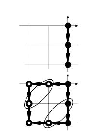
Figure 13: Graph without a hole and
                  graph with a hole

Then we obtain

$$\left({}^{\#}\{A_{z_{1}}\}+{}^{\#}\{A_{z_{2}}\}+{}^{\#}\{q\}\right)-\left({}^{\#}\{\mbox{Eq.(\ref{aarn})}\}+{}^{\#}\{\mbox{Eq.(\ref{aacn})}\}+{}^{\#}\{U(1)\}\right)$$ (147)

$$= 2{}^{\#}\{\mbox{segments}\}+2-2{}^{\#}\{\mbox{points}\}-{}^{\#}\{\mbox{Eq.(\ref{aacn})}\}$$

$$\leq -2\left({}^{\#}\{\mbox{points}\}-{}^{\#}\{\mbox{segments}\}+{}^{\#}\{\mbox{faces}\}\right)+2$$

$$= -2+2$$

$$= 0.$$

From this, we find that if and only if $C_{{\cal I}(l)}$ is a Young diagram, we can have a solution to (137),(138), and that the solution is an isolated one.

Now let us turn to a case, where $C_{{\cal I}(l)}$ has some holes. A diagrams with holes is constructed from one without holes by adding pieces of diagrams. For example, see Fig.13. In Fig.13, some white dots are added to make a hole. Under this operation, the number of undetermined variables increases by

$$\Delta\ {}^{\#}\{\mbox{undetermined variables}\}=\Delta\ {}^{\#}\{A_{z_{1}}\}+\Delta\ {}^{\#}\{A_{z_{2}}\}=2\times 4+2\times 2=12.$$ (148)

On the other hand, the number of constraints increases by

$$\Delta\ {}^{\#}\{\mbox{constraints}\}=\Delta\ {}^{\#}\{\mbox{Eq.(\ref{aarn})}\}+\Delta\ {}^{\#}\{\mbox{Eq.(\ref{aacn})}\}+\Delta\ {}^{\#}\{U(1)\}=5+2\times 2+5=14.$$ (149)

As implied by the above example, one can show that “puncture” operations make the number of constraints greater than that of undetermined variables in general. We conclude that if $C_{{\cal I}(l)}$ has some holes, then (137),(138) have no solution.

We have finished the proof for Theorem3. $\blacksquare$

As mentioned in the top of this section, we have shown that (53),(54),(55),(61),(62) have only isolated solutions, and the solutions are expressed by the Young diagrams.

At the end of this section, we comment on the case that the $q$ are not square matrices. Let us compare above cases with the case of ${\mathbb{C}}^{[n]}$ and the ADHM data for usual U(N) instanton. We have investigated the case that $q_{\dot{\alpha}}$ and $q_{\dot{\alpha}}^{\dagger}$ are $N\times N$ square matrices. It is clear that the above theorem is valid even if $q_{\dot{\alpha}}$ and $q_{\dot{\alpha}}^{\dagger}$ are $N\times k$ and $k\times N$ for arbitrary $k\in{\mathbb{Z}}$, respectively. In this case, our equations (53) - (54) are ADHM equations corresponding to U(N) instanton of $k$ instanton number with Dirac equation reduced to $0$ dimension. The Dirac equation (55) makes no nontrivial equations when we introduce $\zeta$. Then, our models are completely equivalent to the case of ADHM equations with fixed point equations of torus action, that is discussed in Nakajima’s lecture note [49] and others [7, 13, 15]. The proof for the correspondence with ADHM data and the Young diagrams is given by [49]. In this light, our proof in this section is a new version for the Nakajima’s theorem. We solved the fixed point equation of the torus action directly. By virtue of the concrete solution, the correspondence between fields components, ADHM equations and Young diagrams are clarified.

6 Localization Theorem

Though, in this paper, we does not perform the summation of the solutions nor obtain the partition function of our model, we make comment on the localization theorem [39]-[44], which is a powerful tool for the calculation of path integral of cohomological field theories, in order to explain our motivation. To carry out the calculation of infinite $N$ case, that is N.C.${\mathbb{R}}^{4}$ case, is difficult. Therefore we consider the toy model that is given by the same type Lagrangian of section 2 but its all fields are finite $N\times N$ matrices.

For our purpose, one of the most suitable expression of the localization theorem is one given in [9, 16]. This is expressed as follows.

Let ${\tilde{\delta}}$ be the deformed BRS transformation defined in section 4. As explained in section 2, the action $S$ is given by a BRS exact function. Now we redefine the action as

$$S={\tilde{\delta}}\Psi(\phi,{\cal B},{\cal F}).$$ (150)

The difference between ${\hat{\delta}}\Psi$ and ${\tilde{\delta}}\Psi$ causes no effect to the path integral, because the integral of equivariant cohomology is equal to that of original cohomology. Here we have used the notation ${\cal B},{\cal F}$ to denote the BRS doublet fields collectively. Then the localization theorem tells us that

$$Z=\int\frac{D\phi}{U(N)}D{\cal B}D{\cal F}e^{-{\tilde{\delta}}\Psi}=\int\prod_{I=1}^{N}d\phi_{I}\frac{\prod_{I\neq J}(\phi_{I}-\phi_{J})}{Sdet^{\frac{1}{2}}{\cal L}}.$$ (151)

$\phi_{I}$ are the eigenvalues of $\phi$, and the superdeterminant $Sdet{\cal L}$ is defined by

$$Sdet{\cal L}=Sdet\left(\begin{array}[]{cc}\frac{\partial(Q)_{\cal B}}{\partial{\cal F}}&\frac{\partial(Q)_{\cal B}}{\partial{\cal B}}\\ \frac{\partial(Q)_{\cal F}}{\partial{\cal F}}&\frac{\partial(Q)_{\cal F}}{\partial{\cal B}}\end{array}\right),$$ (152)

where $(Q)_{\cal B}$ and $(Q)_{\cal F}$ are defined by the representation of the deformed BRS transformation ${\tilde{\delta}}$ on the fields ${\cal B},{\cal F}$,

$$Q=(Q)_{\cal B}\frac{\partial}{\partial{\cal B}}+(Q)_{\cal F}\frac{\partial}{\partial{\cal F}}.$$ (153)

Note that this expression is analogue of

$${\tilde{d}}=d+i_{X},$$ (154)

where $X$ is a vector defining the Lie derivative ${\cal L}_{X}$ associated with ${\cal G}\otimes T^{N+2}$ action. See (50),(51),(52). In our case, we obtain

$$Z = \int\prod_{I=1}^{N}d\phi_{I}\prod_{I\neq J}(\phi_{I}-\phi_{J})\prod_{I=1}^{N}\frac{(\epsilon_{1}+\epsilon_{2})\{-(\phi_{I}-b_{I})^{2}+\epsilon_{-}^{2}\}}{\epsilon_{1}\epsilon_{2}\{-(\phi_{I}-b_{I})^{2}+\epsilon_{+}^{2}\}}$$ (155)

$$\prod_{I\neq J}\frac{\{(\phi_{I}-\phi_{J})^{2}-4\epsilon_{+}^{2}\}^{\frac{1}{2}}\{-(\phi_{I}-b_{J})^{2}+\epsilon_{-}^{2}\}}{\{-(\phi_{I}-b_{J})^{2}+\epsilon_{+}^{2}\}\{(\phi_{I}-\phi_{J})^{2}-\epsilon_{1}^{2}\}^{\frac{1}{2}}\{(\phi_{I}-\phi_{J})^{2}-\epsilon_{2}^{2}\}^{\frac{1}{2}}},$$

where $\epsilon_{-}=(\epsilon_{1}-\epsilon_{2})/2$.

Some comments might be necessary. This formula is derived by using a some version of localization theorem, which reduces the integral $\int D{\cal B}D{\cal F}$, and this is valid only if the BPS equations of the action (53),(54),(55) and the fixed point equations of the deformed BRS symmetry (61),(62) have isolated solutions for a given value of $\phi_{I}$’s. The integral $\int\prod_{I}d\phi_{I}$ is remained, and this should be understood as the contour integral. In order to define an appropriate contour, we use $\epsilon_{i}\rightarrow\epsilon_{i}+i0$ prescription. The poles correspond to the isolated solutions [39]-[42].

7 Conclusion

The solutions of the Seiberg-Witten monopole equations reduced to $0$ dimension which also satisfy the fixed point equations of torus actions were classified, where the torus action is induced from the global symmetries. More concretely speaking, we deformed the BRS transformation of the topological twisted ${\cal N}=2$ gauge theory on ${\mathbb{R}}^{4}$ with a hypermultiplet to the T-equivariant derivative by using the global symmetries. The global symmetries contain torus actions. Using these symmetries, the deformed BRS transformation was defined to satisfy the nilpotency up to the Lie derivative of the group actions. Then we classified the solutions of the fixed point equations of these deformed BRS transformations.

We showed that the Seiberg-Witten monopole equations are reduced to the ADHM equations with the Dirac equation reduced to $0$ dimension at the large N.C. parameter limit. These equations are described by using infinite dimensional matrices. We showed that the Dirac equation reduced to $0$ dimension is trivial when the ADHM equations and the fixed point equations are satisfied. It is known that the solutions of the ADHM equations with the fixed point equations are isolated ones, and are classified by the Young diagrams, when matrix size is finite. We gave a new proof of this statement, too. Then, we found that we can perform the path integral by using the localization formula, in order to get the partition functions of the finite dimensional matrix model. This finite dimensional matrix model is given as reduced theory to $0$ dimension from the topological twisted ${\cal N}=2$ non-Abelian gauge theory on ${\mathbb{R}}^{4}$ with a hypermultiplet, because the size of matrix is truncated to finite dimension from infinite dimension. We gave the result of the partition function of this toy model. The complete calculation of the partition function for the ${\cal N}=2$ $U(1)$ gauge theory on N.C. ${\mathbb{R}}^{4}$ is remained. This calculation might reveal the relation between the Seiberg-Witten monopole and the instanton. We hope to report on this task elsewhere.

Appendix A Convention

A.1 Complex coordinate

We define the complex coordinate $z^{i},{\bar{z}}^{i}\ (i=1,2)$ as

$$z^{1}=\frac{1}{\sqrt{2}}(x^{1}+ix^{2})\ ,\ {\bar{z}}^{1}=\frac{1}{\sqrt{2}}(x^{1}-ix^{2})\ \ ,$$

$$z^{2}=\frac{1}{\sqrt{2}}(x^{3}+ix^{4})\ ,\ {\bar{z}}^{2}=\frac{1}{\sqrt{2}}(x^{3}-ix^{4})\ \ .$$ (156)

Also, $\partial_{z^{i}},\partial_{{\bar{z}}^{i}}$ are given by

$$\partial_{z^{1}}=\frac{1}{\sqrt{2}}(\partial_{1}-i\partial_{2})\ ,\ \partial_{{\bar{z}}^{1}}=\frac{1}{\sqrt{2}}(\partial_{1}+i\partial_{2})\ \ ,$$

$$\partial_{z^{2}}=\frac{1}{\sqrt{2}}(\partial_{3}-i\partial_{4})\ ,\ \partial_{{\bar{z}}^{2}}=\frac{1}{\sqrt{2}}(\partial_{3}+i\partial_{4})\ \ .$$ (157)

Then, we obtain

$$\partial_{z^{i}}z^{j}=\delta_{i}^{j}\ ,\ \partial_{{\bar{z}}^{i}}{\bar{z}}^{j}=\delta_{i}^{j}\ \ .$$ (158)

A.2 Spinor index

$\epsilon^{\alpha\beta}$,$\epsilon^{{\dot{\alpha}}{\dot{\beta}}}$ and $\epsilon_{\alpha\beta}$,$\epsilon_{{\dot{\alpha}}{\dot{\beta}}}$ are defined by

$$\epsilon^{\alpha\beta}=\epsilon^{{\dot{\alpha}}{\dot{\beta}}}=\left(\begin{array}[]{cc}0&+1\\ -1&0\end{array}\right)\ ,\ \epsilon_{\alpha\beta}=\epsilon_{{\dot{\alpha}}{\dot{\beta}}}=\left(\begin{array}[]{cc}0&-1\\ +1&0\end{array}\right)\ \ .$$ (159)

In other words, $\epsilon_{\alpha\beta}$,$\epsilon_{{\dot{\alpha}}{\dot{\beta}}}$ are defined to be the inverses of $\epsilon^{\alpha\beta}$,$\epsilon^{{\dot{\alpha}}{\dot{\beta}}}$,

$$\epsilon^{\alpha\beta}\epsilon_{\beta\gamma}=\delta^{\alpha}_{\gamma}\ ,\ \epsilon^{{\dot{\alpha}}{\dot{\beta}}}\epsilon_{{\dot{\beta}}{\dot{\gamma}}}=\delta^{\dot{\alpha}}_{\dot{\gamma}}\ \ .$$ (160)

Then a spinor with upper indices and a spinor with lower indices are related as,

$$\psi^{\alpha}=\epsilon^{\alpha\beta}\psi_{\beta}\ ,\ \psi_{\alpha}=\epsilon_{\alpha\beta}\psi^{\beta}\ \ ,$$

$$\psi^{\dot{\alpha}}=\epsilon^{{\dot{\alpha}}{\dot{\beta}}}\psi_{\dot{\beta}}\ ,\ \psi_{\dot{\alpha}}=\epsilon_{{\dot{\alpha}}{\dot{\beta}}}\psi^{\dot{\beta}}\ \ .$$ (161)

We use the following definition for the $4$ dimensional Pauli matrix $\sigma^{\mu}\ (\mu=1,2,3,4)$,

$$(\sigma^{\mu})_{\alpha{\dot{\alpha}}}=\left(\sigma^{1},\sigma^{2},\sigma^{3},\sigma^{4}\right)=\left(i{\bf 1}\ ,\ -{\vec{\tau}}\right)\ ,$$

$$({\bar{\sigma}}^{\mu})^{{\dot{\alpha}}\alpha}=\left({\bar{\sigma}}^{1},{\bar{\sigma}}^{2},{\bar{\sigma}}^{3},{\bar{\sigma}}^{4}\right)=\left(i{\bf 1}\ ,\ +{\vec{\tau}}\right)\ ,$$ (162)

where

$${\vec{\tau}}=\left(\left(\begin{array}[]{cc}0&+1\\ +1&0\end{array}\right),\left(\begin{array}[]{cc}0&-i\\ +i&0\end{array}\right),\left(\begin{array}[]{cc}+1&0\\ 0&-1\end{array}\right)\right)\ .$$ (163)

We define $\sigma^{\mu\nu},{\bar{\sigma}}^{\mu\nu}$ as

$${(\sigma^{\mu\nu})_{\alpha}}^{\beta}=\frac{i}{4}{\left(\sigma^{\mu}{\bar{\sigma}}^{\nu}-\sigma^{\nu}{\bar{\sigma}}^{\mu}\right)_{\alpha}}^{\beta}\ ,$$

$${({\bar{\sigma}}^{\mu\nu})^{\dot{\alpha}}}_{\dot{\beta}}=\frac{i}{4}{\left({\bar{\sigma}}^{\mu}\sigma^{\nu}-{\bar{\sigma}}^{\nu}\sigma^{\mu}\right)^{\dot{\alpha}}}_{\dot{\beta}}\ .$$ (164)

From this definition, $\sigma^{\mu\nu}$ and ${\bar{\sigma}}^{\mu\nu}$ satisfy the anti selfdual relation and the selfdual relation respectively,

$$\sigma^{\mu\nu}=-*\sigma^{\mu\nu}\ ,\ {\bar{\sigma}}^{\mu\nu}=+*{\bar{\sigma}}^{\mu\nu}\ \ .$$ (165)

A.3 $\dagger$ symbol

For a scalar matrix $M$ and a vector matrix $M_{\mu}$, the symbol $\dagger$ denotes the usual hermite conjugation for them,

$$M^{\dagger}=M^{*T}\ ,\ {M_{\mu}}^{\dagger}={M_{\mu}}^{*T},$$ (166)

where the symbol $*$ denotes the complex conjugation and the symbol $T$ denotes the transposition. On the other hand, for an undotted spinor matrix $M_{\alpha}$ and a dotted spinor matrix $M_{\dot{\alpha}}$, ${M_{\alpha}}^{\dagger}$ and ${M_{\dot{\alpha}}}^{\dagger}$ are defined by,

$${M_{\alpha}}^{\dagger}=\epsilon^{\alpha\beta}{M_{\beta}}^{*T}\ ,\ {M_{\dot{\alpha}}}^{\dagger}=\epsilon^{{\dot{\alpha}}{\dot{\beta}}}{M_{\dot{\beta}}}^{*T}\ \ .$$ (167)

This definition makes ${M_{\alpha}}^{\dagger}$ and ${M_{\dot{\alpha}}}^{\dagger}$ to transform in the same rules as $M_{\alpha}$ and $M_{\dot{\alpha}}$ under $SU(2)_{L}$ and $SU(2)_{R(R^{\prime})}$ respectively.

References

- [1] N. Seiberg and E. Witten, Monopole Condensation, And Confinement In N=2 Supersymmetric Yang-Mills Theory, Nucl.Phys. B426 (1994) 19-52, hep-th/9407087.
- [2] N. Seiberg and E. Witten, Monopoles, Duality and Chiral Symmetry Breaking in N=2 Supersymmetric QCD, Nucl.Phys. B431 (1994) 484-550, hep-th/9408099.
- [3] W. Lerche, Introduction to Seiberg-Witten Theory and its Stringy Origin, Nucl.Phys.Proc.Suppl. 55B (1997) 83-117, Fortsch.Phys. 45 (1997) 293-340, hep-th/9611190.
- [4] E. Witten, Monopoles and Four-Manifolds, Math.Res.Lett. 1 (1994) 769-796, hep-th/9411102.
- [5] E. Witten, Yang-Mills Theory on a Four Manifolds, J.Math.Phys.35 (1994) 5101.
- [6] N. Dorey, T.J. Hollowood, V.V. Khoze and M.P. Mattis, The Calculus of Many Instantons, Phys.Rept. 371 (2002) 231-459, hep-th/0206063.
- [7] N. A. Nekrasov, Seiberg-Witten prepotential from instanton counting, Adv.Theor.Math.Phys. 7 (2004) 831-864, hep-th/0206161.
- [8] R. Flume and R. Poghossian, An Algorithm for the Microscopic Evaluation of the Coefficients of the Seiberg-Witten Prepotential, Int.J.Mod.Phys. A18 (2003) 2541, hep-th/0208176.
- [9] U. Bruzzo, F. Fucito, J. F. Morales and A. Tanzini, Multi-Instanton Calculus and Equivalent Cohomology, JHEP 0305(2003)054, hep-th/0211108.
- [10] A. Iqbal and A.-K. Kashani-Poor, Instanton Counting and Chern-Simons Theory, Adv.Theor.Math.Phys. 7 (2004) 457-497, hep-th/0212279.
- [11] A. S. Losev, A. Marshakov and N. A. Nekrasov, Small Instantons, Little Strings and Free Fermions, hep-th/0302191.
- [12] A. Iqbal and A.-K. Kashani-Poor, SU(N) Geometries and Topological String Amplitudes, hep-th/0306032.
- [13] H. Nakajima and K. Yoshioka, Instanton counting on blowup. I. 4-dimensional pure gauge theory, math.AG/0306198.
- [14] A. Hanany and D. Tong, Vortices, Instantons and Branes, JHEP 0307 (2003) 037, hep-th/0306150.
- [15] N. Nekrasov and A. Okounkov, Seiberg-Witten theory and random partitions, hep-th/0306238.
- [16] U. Bruzzo and F. Fucito, Superlocalization Formulas and Supersymmetric Yang-Mills Theories, Nucl. Phys. B 678 (2004) 638, math-ph/0310036.
- [17] T. Eguchi and H. Kanno, Topological Strings and Nekrasov’s formulas, JHEP 0312 (2003) 006, hep-th/0310235.
- [18] T. J. Hollowood, A. Iqbal and C. Vafa, Matrix Models, Geometric Engineering and Elliptic Genera, hep-th/0310272.
- [19] Y. Konishi and K. Sakai, Asymptotic Form of Gopakumar-Vafa Invariants from Instanton Counting, Nucl.Phys. B682 (2004) 465-483, hep-th/0311220.
- [20] A. Iqbal, N. Nekrasov, A. Okounkov and C. Vafa, Quantum Foam and Topological Strings, hep-th/0312022.
- [21] Y. Konishi, Topological Strings, Instantons and Asymptotic Forms of Gopakumar-Vafa Invariants, hep-th/0312090.
- [22] T. Eguchi and H. Kanno, Geometric transitions, Chern-Simons gauge theory and Veneziano type amplitudes, Phys.Lett. B585 (2004) 163-172, hep-th/0312234.
- [23] Y. Tachikawa, Five-dimensional Chern-Simons terms and Nekrasov’s instanton counting, JHEP 0402 (2004) 050, hep-th/0401184.
- [24] A. Marshakov, Strings, Integrable Systems, Geometry and Statistical Models, hep-th/0401199.
- [25] R. Flume, F. Fucito, J. F. Morales and R. Poghossian, Matone’s Relation in the Presence of Gravitational Couplings, JHEP 0404 (2004) 008, hep-th/0403057.
- [26] M. Marino and N. Wyllard, A note on instanton counting for N=2 gauge theories with classical gauge groups, JHEP 0405 (2004) 021, hep-th/0404125.
- [27] N. Nekrasov and S. Shadchin, ABCD of instantons, Commun.Math.Phys. 252 (2004) 359-391, hep-th/0404225.
- [28] G. Bertoldi, S. Bolognesi, M. Matone, L. Mazzucato and Y. Nakayama, The Liouville Geometry of N=2 Instantons and the Moduli of Punctured Spheres, JHEP 0405 (2004) 075, hep-th/0405117.
- [29] H. Fuji and S. Mizoguchi, Gravitational Corrections for Supersymmetric Gauge Theories with Flavors via Matrix Models, Nucl.Phys. B698 (2004) 53-91, hep-th/0405128.
- [30] T. Matsuo, S. Matsuura and K. Ohta, Large N limit of 2D Yang-Mills Theory and Instanton Counting, JHEP 0503 (2005) 027, hep-th/0406191.
- [31] F. Fucito, J. F. Morales and R. Poghossian, Multi instanton calculus on ALE spaces, Nucl.Phys. B703 (2004) 518-536, hep-th/0406243.
- [32] F. Fucito, J. F. Morales and R. Poghossian, Instantons on Quivers and Orientifolds, JHEP 0410 (2004) 037, hep-th/0408090.
- [33] T. Maeda, T. Nakatsu, K. Takasaki and T. Tamakoshi, Five-Dimensional Supersymmetric Yang-Mills Theories and Random Plane Partitions, JHEP 0503 (2005) 056, hep-th/0412327.
- [34] T. Maeda, T. Nakatsu, K. Takasaki and T. Tamakoshi, Free Fermion and Seiberg-Witten Differential in Random Plane Partitions, Nucl.Phys. B715 (2005) 275-303, hep-th/0412329.
- [35] H. Awata and H. Kanno, Instanton counting, Macdonald function and the moduli space of D-branes, JHEP 0505 (2005) 039, hep-th/0502061.
- [36] S. Matsuura and K. Ohta, Localization on D-brane and Gauge theory/Matrix model, hep-th/0504176.
- [37] T. Maeda, T. Nakatsu, Y. Noma and T. Tamakoshi, Gravitational Quantum Foam and Supersymmetric Gauge Theories, hep-th/0505083.
- [38] F.Fucito, J.F.Morales, R.Poghossian and A.Tanzini, N=1 Superpotentials from Multi-Instanton Calculus, hep-th/0510173.
- [39] A. Losev, N. Nekrasov and S. Shatashvili, Issues in Topological Gauge Theory, Nucl.Phys. B534 (1998) 549-611, hep-th/9711108.
- [40] G.Moore, N.Nekrasov and S.Shatashvili, Integrating Over Higgs Branches, Commun.Math.Phys. 209 (2000) 97-121, hep-th/9712241.
- [41] A. Losev, N. Nekrasov and S. Shatashvili, Testing Seiberg-Witten Solution, hep-th/9801061.
- [42] G. Moore, N. Nekrasov and S. Shatashvili, D-particle bound states and generalized instantons, Commun.Math.Phys. 209 (2000) 77-95, hep-th/9803265.
- [43] J.J. Duistermaat and G.J. Heckman, Invent. Math. 69 (1982) 259.
- [44] M. Atiyah and R. Bott, Topology 23 No 1 (1984) 1.
- [45] A.Sako and T. Suzuki, Partition functions of Supersymmetric Gauge Theories in Noncommutative and their Unified Perspective, hep-th/0503214.
- [46] A. Sako, S-I. Kuroki and T. Ishikawa, Noncommutative Cohomological Field Theory and GMS soliton, J.Math.Phys.43(2002)872-896, hep-th/0107033.
- [47] A. Sako, S-I. Kuroki and T. Ishikawa, Noncommutative-shift invariant field theory, proceeding of 10th Tohwa International Symposium on String Theory, (AIP conference proceedings 607, 340).
- [48] A.Sako, Noncommutative Cohomological Field Theories and Topological Aspects of Matrix models, hep-th/0312120.
- [49] H. Nakajima, Lectures on Hilbert Schemes of Points on Surfaces, AMS University Lectures Series, 1999.
- [50] S. Hyun, J. Park and J.-S. Park, Topological QCD, Nucl.Phys. B453 (1995) 199-224, hep-th/9503201.
- [51] S. Hyun, J. Park and J.-S. Park, N=2 Supersymmetric QCD and Four Manifolds; (I) the Donaldson and the Seiberg-Witten Invariants, hep-th/9508162.
- [52] M. Alvarez and J.M.F. Labastida, Topological Matter in Four Dimensions, Nucl. Phys. B437 (1995) 356-390, hep-th/9404115.
- [53] J.M.F. Labastida and M. Marino, A Topological Lagrangian for Monopoles on Four-Manifolds, Phys. Lett. B351 (1995) 146, hep-th/9503105.
- [54] J.M.F. Labastida and M. Marino, Non-Abelian Monopoles on Four-Manifolds, Nucl. Phys. B448 (1995) 373-398, hep-th/9504010.
- [55] E. Witten, Topological quantum field theory, Commun.Math.Phys.117 (1988) 353.
- [56] E. Witten, Introduction to cohomological field theories, Int.J.Mod.Phys.A.6 (1991) 2273.
- [57] A. D. Popov, A. G. Sergeev and M. Wolf, Seiberg-Witten Monopole Equations on Noncommutative , J.Math.Phys. 44 (2003) 4527-4554, hep-th/0304263.
- [58] O. Lechtenfeld, A. D. Popov and R. J. Szabo, Noncommutative Instantons in Higher Dimensions, Vortices and Topological K-Cycles, JHEP 0312 (2003) 022, hep-th/0310267.
- [59] L. Baulieu and H. Kanno and I. M. Singer, Special Quantum Field Theories In Eight and Other Dimensions, Commun.Math.Phys. 194 (1998) 149-175, hep-th/9704167.
- [60] I. Pesando, On the Effective Potential of the Dp- anti Dp system in type II theories, Mod.Phys.Lett. A14 (1999) 1545-1564, hep-th/9902181.
- [61] C. Kennedy and A. Wilkins, Ramond-Ramond Couplings on Brane-Antibrane Systems, Phys.Lett. B464 (1999) 206-212, hep-th/9905195.
- [62] T. Takayanagi, S. Terashima and T. Uesugi, Brane-Antibrane Action from Boundary String Field Theory, JHEP 0103 (2001) 019, hep-th/0012210.
- [63] M. Alishahiha, H. Ita and Y. Oz, On Superconnections and the Tachyon Effective Action, Phys.Lett. B503 (2001) 181-188, hep-th/0012222.
- [64] T. Suyama, BPS Vortices in Brane-Antibrane Effective Theory, hep-th/0101002.
- [65] R. J. Szabo, Superconnections, Anomalies and Non-BPS Brane Charges, J.Geom.Phys. 43 (2002) 241-292, hep-th/0108043.