Abstract

This note is based on a talk given by one of the authors at the ”Rencontres Mathématiques de Glanon”, held in Glanon in July 2004. We will first introduce the BTZ black hole, solution of Einstein’s gravity in 2+1 dimensions, and emphasize some remarkable properties of its geometry. We will essentially pay attention to the non-rotating black hole, whose structure is significantly different to the generic case. We will then turn the some aspects of string theory, namely the emergence of non-commutative geometry and the embedding of the BTZ black hole as an exact string background using the Wess-Zumino-Witten (WZW) model. We will show the existence of winding symmetric WZW D1-branes in this space-time from the geometrical properties of the non-rotating black hole. Finally, we will introduce strict deformations of these spaces, yielding an example of non-commutative lorentzian non-compact space, with non-trivial causal structure.

1 Geometry of the BTZ black holes

Vacuum Einstein’s equations in 2+1 dimensions with negative cosmological constant admit black hole solutions, as first quoted in [1]. A remarkable property of these solutions lies in the fact that they arise from identifications of points of $AdS_{3}$ by a discrete subgroup of its isometry group, as shown by Bañados, Henneaux, Teitelboim and Zanelli [2, 3]. They are therefore usually referred to as BTZ black holes in the physics literature. According to the type of subgroup, the vacuum, extremal or generic (rotating or non-rotating) massive black holes are obtained.

1.1 Three-dimensional anti-de Sitter space

The three dimensional anti de-Sitter space ($AdS_{3}$) is the maximally symmetric solution of vacuum Einstein’s equation in 2+1 dimensions with negative cosmological constant $\Lambda$. It is defined as the hyperboloid

$$u^{2}+t^{2}-x^{2}-y^{2}=-1/\Lambda\quad,$$ (1.1)

embedded in the four dimensional flat space with metric $ds^{2}=-du^{2}-dt^{2}+dx^{2}+dy^{2}$. The Ricci tensor of this solution satisfies $R_{\mu\nu}=2\Lambda g_{\mu\nu}$ and the scalar curvature is $R=6\Lambda$. Hereafter, we will set $\Lambda=-1$.

It follows from (1.1) that $AdS_{3}$ can equivalently by defined as the (universal covering of) the simple Lie group $\mbox{SL}(2,\mathbb{R})$ :

$$AdS_{3}\cong\mbox{SL}(2,\mathbb{R})=\{g=\left(\begin{array}[]{cc}u+x&y+t\\ y-t&u-x\end{array}\right)|x,y,u,t\in\mathbb{R},\ \det g=1\}\qquad.$$ (1.2)

We endow $\mbox{SL}(2,\mathbb{R})$ with its bi-invariant Killing metric, defined at the identity $e$ using the Killing form $B$ of its Lie algebra $sl(2,\mathbb{R})$, identified with the tangent space at the identity:

$$\beta_{e}(X,Y)=B(X,Y)=\frac{1}{2}\mbox{Tr}(X.Y)\quad,X,Y\in sl(2,\mathbb{R})\quad,$$ (1.3)

where the last equality holds because we are dealing with a matrix group, the trace being understood as the usual matricial one (i.e. in the fundamental representation). It can be checked, given a parametrization $g(X^{\mu})$ of the group manifold , that the invariant metric $\mbox{Tr}(g^{-1}dgg^{-1}dg)$ actually coincides with the $AdS_{3}$ metric (see sect.1.1.2). The Lie algebra

$$sl(2,\mathbb{R})=\{\left(\begin{array}[]{cc}z^{H}&z^{E}\\ z^{F}&-z^{H}\end{array}\right):=z^{H}\,{\bf H}+z^{E}\,{\bf E}+z^{F}\,{\bf F}\}\qquad,$$ (1.4)

is expressed in terms of the generators $\{\,{\bf H},\,{\bf E},\,{\bf F}\}$ satisfying the commutation relations:

$$[\,{\bf H},\,{\bf E}]=2\,{\bf E}\quad,\quad[\,{\bf H},\,{\bf F}]=-2\,{\bf F}\quad,\quad[\,{\bf E},\,{\bf F}]=\,{\bf H}\quad.$$ (1.5)

For later purpose, we also define the one-parameter subgroups of $\mbox{SL}(2,\mathbb{R})$ :

$$A=\exp(\mathbb{R}\,\,{\bf H})\ ,\quad N=\exp(\mathbb{R}\,\,{\bf E})\ ,\quad K=\exp(\mathbb{R}\,\,{\bf T})\ ,\ \qquad,$$ (1.6)

which are the building blocks of its Iwasawa decomposition (see [5, 6]) :

$$K\times A\times N\rightarrow\mbox{SL}(2,\mathbb{R})(2,\mathbb{R}):(k,a,n)\rightarrow kan\,\,\mbox{or}\,\,ank\,,\,k\in K,\,a\in A,\,n\in N\quad,$$ (1.7)

the mapping being an analytic diffeomorphism of the product manifold $K\times A\times N$ onto Sl$(2,\mathbb{R})$ (see [6], p.234)

1.1.1 Isometry group of $AdS_{3}$

By construction, the isometry group of $AdS_{3}$, denoted by $Iso(AdS_{3})$, is the four-dimensional Lorentz group $O(2,2)$ (see (1.1)). It is constituted by four connected parts, whose identity component is $SO(2,2)$. The other components can always be reached using a parity ($x\rightarrow-x$) and/or time reversal ($t\rightarrow-t$) transformation. In terms of the coordinates of (1.1), the Killing vector fields are expressed as $J_{ij}=x_{j}\partial_{i}-x_{i}\partial_{j}$, where $x^{i}=(u,t,x,y)$. Now, because of (1.2) and due to the bi-invariance of the Killing metric, $SO(2,2)$ is locally isomorphic to $\mbox{SL}(2,\mathbb{R})\times\mbox{SL}(2,\mathbb{R})$ (they share the same Lie algebra) , the action being given by

$$(\mbox{SL}(2,\mathbb{R})\times\mbox{SL}(2,\mathbb{R}))\times\mbox{SL}(2,\mathbb{R})\rightarrow\mbox{SL}(2,\mathbb{R}):((g_{L},g_{R}),z)\rightarrow g_{L}\,z\,g_{R}^{-1}\quad.$$ (1.8)

This action clearly corresponds to the component of $Iso(AdS_{3})$ connected to the identity transformation (because $\mbox{SL}(2,\mathbb{R})$ is connected). The full action of $Iso(AdS_{3})$ (including the components not connected to the identity) can be obtained by considering the parity and time reversal transformations

$${\cal P}(g) = \left(\begin{array}[]{cc}u-x&y+t\\ y-t&u+x\end{array}\right)\quad,$$ (1.11)

$${\cal T}(g) = \left(\begin{array}[]{cc}u+x&y-t\\ y+t&u-x\end{array}\right)\quad.$$ (1.14)

There exists a Lie algebra isomorphism between $sl(2,\mathbb{R})\times sl(2,\mathbb{R})$ and $iso(AdS_{3})\equiv Lie(Iso(AdS_{3}))$. It is given by

$$\Phi:sl(2,\mathbb{R})\times sl(2,\mathbb{R})\rightarrow iso(AdS_{3}):(X,Y)\rightarrow\overline{X}-\underline{Y}\quad,$$ (1.15)

where $\overline{X}$ (resp. $\underline{Y}$) denotes the right-invariant (resp. left-invariant) vector field on $\mbox{SL}(2,\mathbb{R})$ associated to the element $X$ (resp. $Y$) of its Lie algebra, that is

$$\overline{X}_{g} = \frac{d}{dt}_{|0}L_{\exp tX}\,g=\frac{d}{dt}_{|0}\exp(tX)\,g=Xg\quad,$$ (1.16)

$$\underline{Y}_{g} = \frac{d}{dt}_{|0}R_{\exp tX}\,g=\frac{d}{dt}_{|0}g\,\exp(tY)=gY\quad,$$ (1.17)

where $L_{g}$ and $R_{g}$ denote the left and right translations on the group manifold. The two last equalities hold because $\mbox{SL}(2,\mathbb{R})$ is a matrix group.

Thus, to the generator $(X,Y)\in sl(2,\mathbb{R})\times sl(2,\mathbb{R})$, we associate the one-parameter subgroup of (the connected part of) $Iso(AdS_{3})$

$$\Psi_{t}(g)=\exp(tX)\,g\,\exp(-tY)\quad,\quad g\in\mbox{SL}(2,\mathbb{R}),t\in\mathbb{R}\quad.$$ (1.18)

The classification, up to conjugation, of the one-parameter subgroups of $\mbox{SL}(2,\mathbb{R})\times\mbox{SL}(2,\mathbb{R})$ has been achieved in [3, 7]. Two subgroups $(G_{L},G_{R})$ and $(G^{\prime}_{L},G^{\prime}_{R})$ are said to be conjugated if

(i) they can be related by combinations of transformations $\cal P$ and $\cal T$;

(ii) there exists $g_{L}$ and $g_{R}$ $\in\mbox{SL}(2,\mathbb{R})$ such that $G_{i}=g_{i}\,G^{\prime}_{i}\,g_{i}^{-1}$, for $i=L,R$. Note that (ii) corresponds to a conjugation by an element of $SO(2,2)$, while (i) corresponds to an element not connected to the identity. The Killing vectors of $AdS_{3}$ (i.e. the generators of the one-parameter subgroups of $\mbox{SL}(2,\mathbb{R})\times\mbox{SL}(2,\mathbb{R})$) are then all of the form

$$(aX,bY),\quad a,b\in\mathbb{R}\quad,\quad X,Y=\{\,{\bf H},\,{\bf T},\,{\bf E},\,{\bf F}\}\quad.$$ (1.19)

1.1.2 Conformal structure/representation

A system of coordinates covering the whole of the $AdS_{3}$ manifold (up to trivial polar singularities) may be introduced by setting

$$u=l\cosh\xi\,\cos\lambda\qquad, t=l\cosh\xi\,\sin\lambda\qquad,$$

$$x=l\sinh\xi\,\cos\varphi\qquad, y=l\sinh\xi\,\sin\varphi\quad,$$ (1.20)

in which the invariant metric on $AdS_{3}$ reads

$$ds^{2}=l^{2}(-\cosh^{2}\xi\,d\lambda^{2}+d\xi^{2}+\sinh^{2}\xi\,d\varphi^{2})\qquad,$$ (1.21)

with $l^{2}=-\frac{1}{\Lambda}$. The further change of radial coordinate:

$$\tanh\xi=\sin r\hskip 28.45274ptr\in[0,\pi/2[\qquad,$$ (1.22)

yields a conformal embedding of $AdS_{3}$ in the Einstein static space [8]:

$$ds^{2}=\frac{l^{2}}{\cos^{2}r}\left(-d\lambda^{2}+dr^{2}+\sin^{2}r\,d\varphi^{2}\right)\qquad.$$ (1.23)

1.2 BTZ black holes

1.2.1 General construction

Einstein gravity with negative cosmological constant in 2+1 dimensions admits axially symmetric and static black hole solutions, characterized by their mass $M$ and angular momentum $J$. One distinguishes between the extremal ($|J|=Ml$), massless ($J=M=0$), non-rotating massive ($J=0$,$\,M>0$) and generic ($0<|J|<Ml$) black holes. These solutions share many common properties with their 3+1 dimensional counterparts. Bañados, Henneaux, Teitelboim and Zanelli observed [3] that all of these solutions could be obtained by performing identifications in $AdS_{3}$ space by means of a discrete subgroup of its isometry group, which we described in section 1.1.1. According to the choice of Killing vector $\Xi=(X_{L},X_{R})$, the different black holes can be obtained by the quotient procedure. The mass and the angular momentum of the solution will be related to $\Xi$ via

$$M(\Xi) = \frac{1}{2}\left(\|X_{L}\|^{2}+\|X_{R}\|^{2}\right)\qquad,$$ (1.24)

$$J(\Xi) = \frac{1}{2}\left(\|X_{L}\|^{2}-\|X_{R}\|^{2}\right)\qquad,$$ (1.25)

where $\|X\|^{2}$ is the square of the Killing norm $\beta_{e}(X,X)$.

In the following, we will focus on the non-rotating massive black hole. In this situation, because of (1.24) and (1.25), $X_{L}$ and $X_{R}$ must belong to the same space-like adjoint orbit.

In this case, we define the BHTZ subgroup as the one-parameter subgroup of $\mbox{SL}(2,\mathbb{R})\times\mbox{SL}(2,\mathbb{R})$ generated by the Killing vector $\Xi=a(\overline{\,{\bf H}}-\underline{\,{\bf H}})=(a\,{\bf H},a\,{\bf H})$ :

$$\psi_{t}(z)=\exp(ta\,{\bf H})\,z\,\exp(-ta\,{\bf H})\,,\quad z\in\mbox{SL}(2,\mathbb{R}).$$ (1.26)

A non-rotating massive BTZ black hole is then obtained as the quotient $\mbox{SL}(2,\mathbb{R})/\psi_{\mathbb{Z}}$ by an isometric action of $\mathbb{Z}$, that is, by performing the following identifications :

$$z\sim\exp(na\,{\bf H})\,z\,\exp(-na\,{\bf H})\quad,\quad n\in\mathbb{Z}\quad.$$ (1.27)

The resulting space-time displays a black hole structure [3]. Namely, it exhibits horizons, i.e. light-like surfaces separating two regions, one of which can be causally connected to the space-like infinity (the exterior region), and another one causally disconnected from it (the interior region). Inside the horizon, any light-ray necessarily ends on the singularity.

Note that, to avoid closed time-like curves in the quotient space, the regions of $AdS_{3}$ where the orbits of the BHTZ action (1.26) are time-like ,or equivalently where $\beta_{z}(\Xi,\Xi)<0$, must be excluded. We will henceforth consider an open and connected domain ${\cal U}\subseteq AdS_{3}$ where $\beta_{z}(a\,{\bf H},a\,{\bf H})>0\quad,\forall z\in{\cal U}$. The black holes singularities ${\cal S}$ are defined as the surfaces where the identifications becomes light-like :

$${\cal S}=\{z\in AdS_{3}\,\,|\,\,\beta_{z}(\Xi,\Xi)=0\}\quad.$$ (1.28)

1.2.2 Massless non-rotating BTZ as twisted bi-quotient space/Global structure

We would now like to focus on the global geometry of the non-rotating massive BTZ black hole [7]. The aim is essentially to reduce ourselves to a two-dimensional problem by finding a foliation of $AdS_{3}$ whose leaves are stable under the BHTZ action, and are all isomorphic (so that we can restrict ourselves to the leaf through the identity). Let us first introduce an external automorphism of ${\mathfrak{sl}(2,\mathbb{R})}{}$, which can be chosen as

$$\sigma(\,{\bf H})=\,{\bf H},\ \sigma(\,{\bf E})=-\,{\bf E},\ \sigma(\,{\bf F})=-\,{\bf F}\qquad.$$ (1.29)

Viewing $\mbox{SL}(2,\mathbb{R})$ as a subgroup of ${GL(2,\mathbb{R})}$, one may express the automorphism $\sigma$ as:

$$\sigma=Ad(\,{\bf H})\qquad\mbox{where}\qquad\,{\bf H}=\left(\begin{array}[]{cc}1&0\\ 0&-1\end{array}\right)\in GL(2,\mathbb{R})\qquad.$$ (1.30)

The corresponding external automorphism of $\mbox{SL}(2,\mathbb{R})$ (which we again denote by $\sigma$) is $\sigma(g)=\,{\bf H}\,g\,{\bf H}$ (note that $\,{\bf H}=\,{\bf H}^{-1}$). We then consider the following twisted action of $\mbox{SL}(2,\mathbb{R})\subset SO(2,2)$ on itself :

$$\mbox{SL}(2,\mathbb{R})\times\mbox{SL}(2,\mathbb{R})\rightarrow\mbox{SL}(2,\mathbb{R}):(g,z)\rightarrow\tau_{g}(z)=g\,z\,\sigma(g^{-1})\quad.$$ (1.31)

The fundamental vector field associated to this action is given by :

$$X^{*}_{z}=\frac{d}{dt}_{|t=0}\tau_{\exp(-tX)}(z)=-Xz+z\sigma(X)\quad,$$ (1.32)

by noting that $\sigma(\exp(tX))=\exp(t\,\sigma(X))$, with an evident abuse of notation. We note that the BHTZ action $\mathbb{Z}\times\mbox{SL}(2,\mathbb{R})$ ( eq.(1.26)) can equivalently be written as

$$\psi_{t}(z)=\tau_{\exp(a\,t\,\,{\bf H})}(z)\quad.$$ (1.33)

The orbit of a point $z$ under this action is

$${\cal O}_{z}=\{\,\,\tau_{g}(z)\quad,\,g\in\mbox{SL}(2,\mathbb{R})\}\quad$$ (1.34)

and is usually referred to as a twisted conjugacy class. This particular structure will become important in section 2 where we will discuss D-branes in Wess-Zumino-Witten models. Using the matrix representation of (1.2), we find that ${\cal O}_{z}$ is constituted by the elements $g\in\mbox{SL}(2,\mathbb{R})$ such that $x(g)=x(z)=cst$. We see from (1.1) that the orbits are two-dimensional one-sheet hyperboloids in flat four-dimensional space. We won’t make use of this representation, but adopt a more convenient one.

The global description of the black hole relies on the following proposition. Consider the application :

$$\phi:K\times A\times N\rightarrow\mbox{SL}(2,\mathbb{R}):(k,a,n)\rightarrow\phi(k,a,n)=\tau_{kn}(a)\quad.$$ (1.35)

This application is a global diffeomorphism. Furthermore, we observe, by letting $g=kna^{\prime}\in\mbox{SL}(2,\mathbb{R})$ that

$$\tau_{g}(a)=\phi(a,n,k)\quad\forall a\in A.$$ (1.36)

Therefore, the orbit of $a\in A$ under the twisted bi-action is given by

$${\cal O}_{a}=\phi(a,N,K)\cong NK=G/A\quad,$$ (1.37)

where the last equality holds because of the Iwasawa decomposition of $G=\mbox{SL}(2,\mathbb{R})$ (1.7). The application can be rewritten as

$$\phi:A\times G/A\rightarrow G:(a,[g])\rightarrow g\,a\,\sigma(g^{-1})\quad,$$ (1.38)

where $[g]=\{gA,\,g\in G\}\in G/A.$ This is exactly the decomposition we needed to reduce the geometrical description of $AdS_{3}$ and the black hole from three to two dimensions. Indeed, it provides us with a foliation (a trivial fibration) of $AdS_{3}$ over $A\simeq\mathbb{R}$ whose leaves are two-dimensional orbits of the action (1.31). Each of the leaves is stable under the BHTZ subgroup, that is, $z\in{\cal O}_{a}\Rightarrow\psi_{t}(z)\in{\cal O}_{a},\,a\in A\,,z\in\mbox{SL}(2,\mathbb{R})$. Moreover, the BHTZ action is fiberwise , which means that

$$\tau_{h}(\phi(a,[g]))=\phi(a,h.[g])=\phi(a,[hg])\quad.$$ (1.39)

This, with the fact that the orbits are all diffeomorphic, allow us to restrict ourselves to the study of the leaf through the identity and focus on the space $G/A$. This space can be realized as the adjoint orbit of $\,{\bf H}$ in ${\mathfrak{sl}(2,\mathbb{R})}{}$. Indeed, consider the application

$$\Upsilon:G/A\rightarrow Ad(G)\,{\bf H}:[g]\rightarrow\Upsilon([g])=Ad(g)\,{\bf H}\quad.$$ (1.40)

Because $Ker\Upsilon=\{[e],[-e]\}$, $G/A$ is a $\mathbb{Z}_{2}$ covering of $Ad(G)\,{\bf H}$. It is well defined because $Ad(a)\,{\bf H}=\,{\bf H}\,\forall a\in A$.

With $A\cong\mathbb{R}$ and using the application $\Upsilon$, $\phi$ can further be rewritten as

$$\phi:\mathbb{R}\times Ad(G)\,{\bf H}\rightarrow G:(\rho,Ad(kn)\,{\bf H})\rightarrow\phi(\rho,Ad(kn)\,{\bf H})=\tau_{kn}(\exp(\rho\,{\bf H}))\quad.$$ (1.41)

Restricting $\phi$ to the leaf at identity ${\cal O}_{e}$ (for which $\rho=0$) , we define the application

$$\iota:Ad(G)\,{\bf H}\rightarrow{\cal O}_{e}:Ad(kn)\,{\bf H}\rightarrow\tau_{kn}(e)\quad,$$ (1.42)

and consider the adjoint orbit of $\,{\bf H}$, which corresponds to a one-sheet hyperboloid in ${\mathfrak{sl}(2,\mathbb{R})}{}$

The orbit of a point $X$ in the hyperboloid (i.e. corresponding to a point $x$ in the leaf at the identity) under the BHTZ subgroup are the intersections of the planes perpendicular to the $\,{\bf H}$-axis, passing through $X$. Indeed, let $X=Ad(kn)\,{\bf H}$, corresponding to the point $x=\tau_{kn}(e)\in{\cal O}_{e}$. The orbit of $x$ under the BHTZ subgroup is

$$\psi_{n}(x)=\tau_{\exp(n\,{\bf H}a)}(x)=\tau_{\exp(n\,{\bf H}a)kn}(e)\quad,$$ (1.43)

corresponding to the curve $Ad(\exp(n\,{\bf H}a))X$ on $Ad(G)\,{\bf H}$. One then checks, using the $Ad$-invariance of the Killing form, that

$$\beta_{e}(\,{\bf H},Ad(\exp(n\,{\bf H}a)X-X)=0\quad.$$ (1.44)

Let us summarize. To obtain the non-rotating massive BTZ black hole space-time, we have to perform discrete identifications in $AdS_{3}$ along the orbits of the BHTZ action, or equivalently of a twisted bi-action (see eq.(1.33)). We know from (1.39) that the identifications can be performed ”leaf by leaf”, all the leaves being diffeomorphic. We also know that, in order to avoid closed time-like curves in the quotient space, we have to restrict ourselves to an open and connected domain ${\cal U}\subseteq AdS_{3}$ where $\beta_{z}(\Xi,\Xi)>0\quad,\forall z\in{\cal U}$. Therefore we have to identify the corresponding region in $Ad(G)\,{\bf H}$. It can be seen that the region where the orbits of the BHTZ action are space-like corresponds to

$$\{X=x^{\,{\bf H}}\,{\bf H}+x^{\,{\bf E}}\,{\bf E}+x^{\,{\bf F}}\,{\bf F}\in Ad(G)\,{\bf H}\quad|\quad-1<x^{\,{\bf H}}<1\}\quad.$$ (1.45)

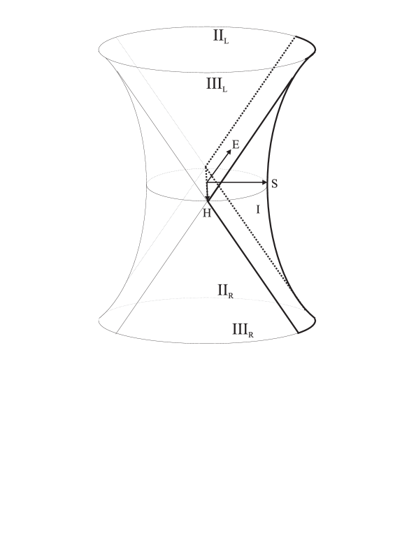
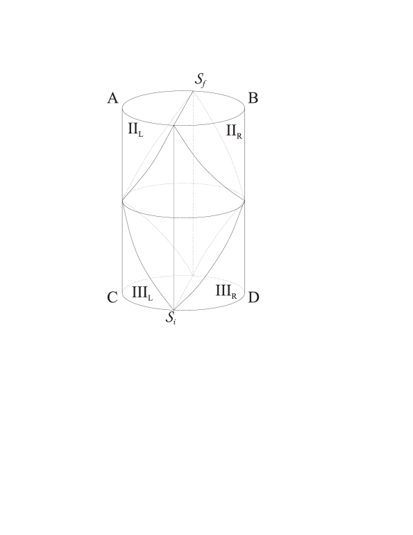
Figure 1: An adjoint orbit of $\,{\bf H}$ under $\mbox{SL}(2,\mathbb{R})$, identified to a leaf of the foliation.The region $I$ corresponds to one region where the BHTZ orbits are space-like.

Figure 2: A conformal picture of $AdS_{3}$, seen as an Einstein cylinder (see eq. (1.23) ). A region where $\Xi$ is space-like (a black hole region) is represented between four light-like surfaces.

One of these regions in represented in figure 2 and labelled $I$. It can be parameterized as

$$X=Ad\left(\exp(\frac{\theta}{2}\,{\bf H})\,\exp(-\frac{\tau}{2}\,{\bf T})\right)\,\,{\bf H}\quad,\,0<\tau<\pi\,,\,-\infty<\theta<+\infty.$$ (1.46)

In this parameterization, the orbits of the BHTZ action are the lines $\tau=cst.$. Using (1.42), any point $x\in{\cal O}_{e}$ belonging to ${\cal U}$ can be parameterized by the two coordinates $(\theta,\tau)$ via

$$z(\theta,\tau)=\tau_{\exp(\frac{\theta}{2})\,{\bf H}\,\exp(-\frac{\tau}{2})\,{\bf T}}(e)$$ (1.47)

Note that $e$ and $-e$ belong to the boundary of ${\cal U}$. Finally, we obtain a global parameterization of points in ${\cal U}$ with the help of (1.38), as

$$z(\rho,\theta,\tau)=\tau_{\exp(\frac{\theta}{2}\,{\bf H})\,\exp(-\frac{\tau}{2}\,{\bf T})}(\exp(\rho\,{\bf H}))\quad.$$ (1.48)

The action of the BHTZ reads in these coordinates

$$(\tau,\rho,\theta)\rightarrow(\tau,\rho,\theta+2na)\quad.$$ (1.49)

Eq. (1.48) allows to derive a global expression for the metric of the black hole :

$$ds^{2}=d\rho^{2}+\cosh^{2}\rho(-d\tau^{2}+\sin^{2}\tau d\theta^{2})\quad,\quad-\infty<\rho<+\infty,\,0<\tau<\pi,\,0<\theta<2a\quad.$$ (1.50)

The black hole has topology $S^{1}\times\mathbb{R}^{2}$.

Let us turn to some pictures displaying the global structure of the black hole. Recall from section 1.1.2 that $AdS_{3}$ is conformal to the three-dimensional Einstein static space. The time axis $\lambda$ (see eq.(1.23)). Fig.2, displays the region ${\cal U}$ where the Killing vector $\Xi$ is space-like, which is comprise between the four light-like surfaces.

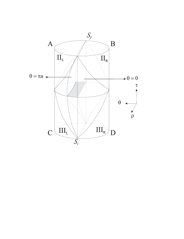
Figure 3: Foliation of $AdS_{3}$ in twisted conjugacy classes ($\rho=cst$ surfaces).

Figure 4: Dynamical evolution of the black hole, from its initial singularity ${\cal S}_{i}$ to the final singularity ${\cal S}_{f}$. The shaded region represents a timelike section of a fundamental domain of the BHTZ action.

The next one (Fig.4) represents the foliation of $AdS_{3}$ by the two-dimensional space-like $\rho=cst.$ leaves.

Figure 4 represents the dynamical evolution of the black hole, from its initial to its final singularity (denoted ${\cal S}_{i}$ and ${\cal S}_{i}$) , using the global coordinates $(\tau,\rho,\theta)$. The shaded region is a fundamental domain of the BHTZ action.

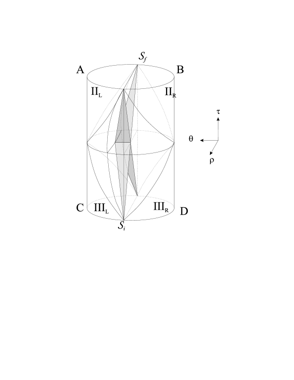
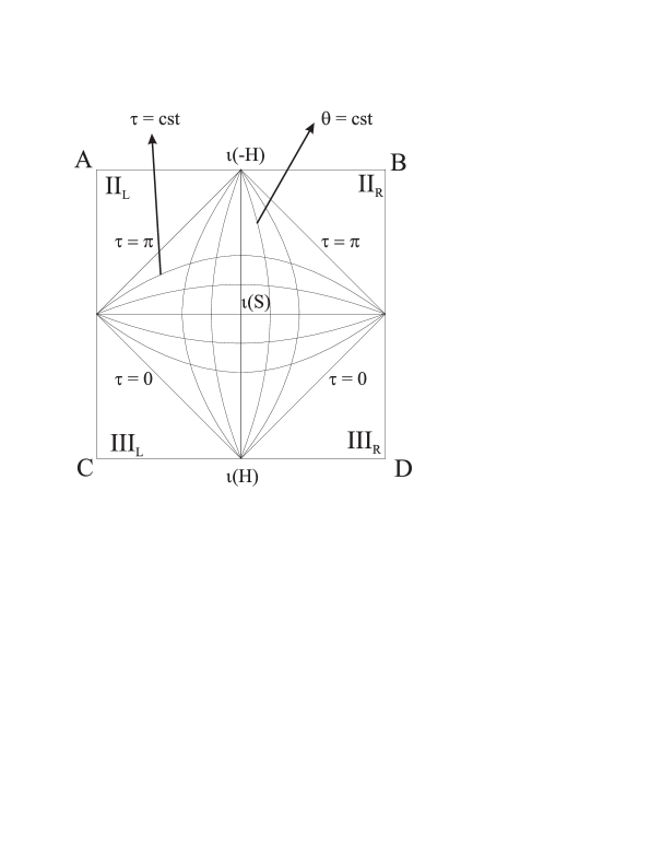
Figure 5: Representation of the black hole’s horizons. These are light-like surfaces separating two regions, one of which can be causally connected to the space-like infinity (the exterior region), and another one causally disconnected from it (the interior region).

Figure 6: A $\rho=0$ section of Fig.2, where the coordinate lines are represented. The orbits of the BHTZ subgroup correspond to $\tau=cst$.

In Fig. 6, the black hole horizons are drawn.

From these three-dimensional pictures, we can also go to two different two-dimensional visions. Fig.(6) is a section of Fig.(2) by the $\rho=0$ surface. We represented the coordinate lines $\theta=cst.$ and $\tau=cst.$ (the latter corresponding to orbits of the BHTZ subgroup). On the straight lines, the identifications become light-like. Note that, after identifications, the manifold structure is destroyed at $e=\iota(\,{\bf H})$ and $-e=\iota(-\,{\bf H})$, which are fixed points of the BHTZ action (see sect.$5.8$ of [8], and [3]). Everywhere else in $I$, the action of the BHTZ subgroup is properly discontinuous.

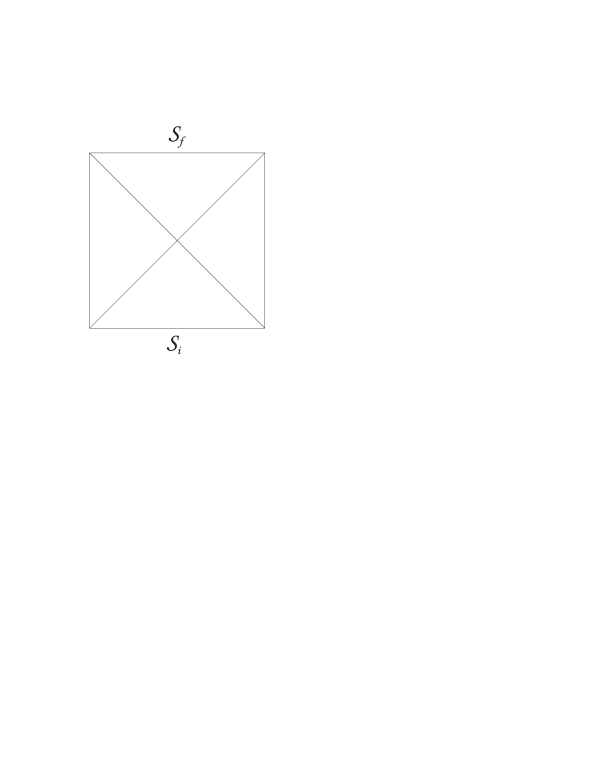
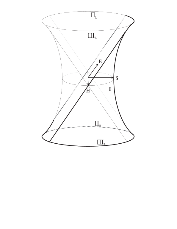
Figure 7: A $\theta=0$ section of Fig.2, yielding a Penrose diagram of the black hole. The oblique lines represent the black hole’s horizons.

Figure 8: The extension we consider, consisting in each leaf in half a hyperboloid. This region exactly coincides with the orbits of an $AN$ subgroup of $\mbox{SL}(2,\mathbb{R})$.

One can also look at the section by the $\theta=0$ surface. One then gets an usual two-dimensional Penrose diagram, where the singularities and horizons are drawn, as displayed in Fig. 8.

1.2.3 Extended BTZ black holes

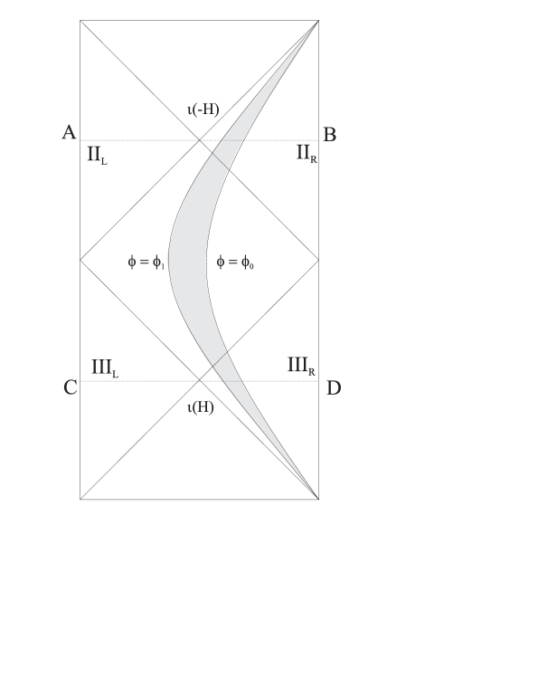
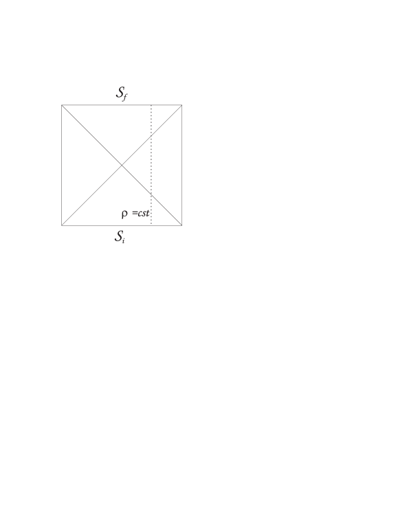
Figure 9: Same section as Fig.6, for the extension we considered. The shaded region corresponds to a section of a fundamental domain of the BHTZ action.

Figure 10: A $\rho=cst.$ D1-brane is represented in this Penrose diagram of the non-rotating massive BTZ black hole, where each point represents a circle. We see the brane emerging from the past singularity, cross the horizons and end on the future singularity. Note that a similar behavior is observed for D0-branes in the $\mbox{SL}(2,\mathbb{R})/U(1)$ two-dimensional black hole (see [43])

If we relax the condition that closed time-like curves must be avoided, while keeping the condition that the quotient space $\mbox{SL}(2,\mathbb{R})/\psi_{\mathbb{Z}}$ be a Hausdorff manifold, there are two inequivalent possibilities to extend the BTZ space-time. Either we choose to consider, in each leaf, the region $I\cup II_{L}\cup III_{R}$, either we take $I\cup II_{R}\cup III_{R}$ (see Figs. 2, 6,10). The latter extension exhibits an interesting property : in this situation, each leaf in the extension admits an action of the two-parameter $AN$ subgroup of $\mbox{SL}(2,\mathbb{R})$. Indeed, we note that the region $I\cup II_{R}\cup III_{R}$ in $Ad(G)\,{\bf H}$ (see Fig. 8) can be parameterized as

$$X=Ad\left(\exp(\frac{\phi}{2}\,{\bf H})\exp(w\,{\bf E})\right)\,{\bf S}\quad,\quad-\infty<\phi<+\infty,\,-\infty<w<+\infty\,,$$ (1.51)

where $\,{\bf S}=Ad\left(\exp(-\frac{\pi}{4})\,{\bf T})\right)\,{\bf H}$.

Therefore, if $x=\tau_{r\exp(-\frac{\pi}{4}\,{\bf T})}\left(\exp(\rho\,{\bf H})\right)\in I\,\cup\,II_{R}\,\cup\,III_{R}\,\subset{\cal O}_{\rho}$, where $r=\exp(\frac{\phi}{2}\,{\bf H})\exp(w\,{\bf E})$, then $\tau_{r^{\prime}}(x)\in I\,\cup\,II_{R}\,\cup\,III_{R}\,\subset{\cal O}_{\rho},\,\forall r^{\prime}\in R=AN$.

A section by the $\rho=0$ surface is depicted in Fig. 10, where two coordinate lines $\theta=cst.$ are drawn. The region in between corresponds to a fundamental domain of the BHTZ action. Hereafter, the maximally extended BTZ space-time whose each leaf is constituted by the regions $I\,\cup\,II_{R}\,\cup\,III_{R}$ will be denoted $EBTZ$.

2 Non-commutative geometry from string theory

2.1 Open strings in flat space-time in presence of constant B-field

There are actually several ways to observe the emergence of non-commutativity by analyzing open string theory in flat space-time in the presence of a constant magnetic field $B$ on a D-brane. We will focus on one of them, namely the direct canonical quantization. Consider an open string propagating in a flat D-dimensional space-time ${\cal M}^{d}$ with metric $\eta_{\mu\nu}$ in presence of a constant $B_{\mu\nu}$. The string worldsheet, i.e. the surface swept out by the string during its temporal evolution, will be parameterized by a set of fields $X^{\mu}:\Sigma\rightarrow{\cal M}^{d}$, where $\Sigma$ is the strip $[0,\pi]\times\mathbb{R}$. The action of the bosonic open string theory in this background geometry, in the conformal gauge, is

$$S=-\frac{1}{4\pi\alpha^{\prime}}\int_{\Sigma}\,d^{2}x\,(\eta_{\mu\nu}+B_{\mu\nu})\,\partial_{+}X^{\mu}\partial_{-}X^{\nu}\quad,$$ (2.52)

where the string tension

is $T=\frac{1}{2\pi\alpha^{\prime}}$, $x_{+}$ and $x_{-}$ are light cone coordinates on the worldsheet. The equations of motion for the string coordinates following from the variation of action (2.52) are given by

$$\partial_{+}\partial_{-}X^{\mu}=0\quad,\quad\mu=0,\cdots,d-1\quad$$ (2.53)

and are not affected by the presence of the constant B-field. By introducing the currents

$$J_{+}^{\mu}=\partial_{+}X^{\mu}\quad\mbox{and}\quad J_{-}^{\mu}=\partial_{-}X^{\mu}\quad,$$ (2.54)

the equations of motion simply state that

$$J_{+}=J_{+}(x^{+})\quad\mbox{and}\quad J_{-}=J_{-}(x^{-})\quad,$$ (2.55)

or, expressed in terms of $z=e^{ix_{-}}$ and $\bar{z}=e^{ix_{+}}$ (see footnote), that the currents

$$J^{\mu}=\partial X^{\mu}\quad\mbox{and}\quad\bar{J}^{\mu}=\bar{\partial}X^{\mu}\quad,$$ (2.56)

are purely holomorphic or anti-holomorphic, respectively. Variation of the action (2.52) shows that the equations of motion (2.53) have to be supplemented by boundary conditions at the boundary of the string worldsheet, which can be satisfied in two different ways :

$$\partial_{\tau}X^{\mu}_{|\sigma=0,\pi}=0\quad.$$ (2.57)

or

$$\left(\eta_{\mu\nu}\partial_{\sigma}X^{n}u-B_{\mu\nu}\partial_{\tau}X^{\nu}\right)_{|\sigma=0,\pi}=0\quad,$$ (2.58)

The first one corresponds to Dirichlet boundary conditions, while the second one corresponds to generalized Neumann conditions (Neumann boundary conditions are recovered for $B=0$). We can impose independently either of the conditions in each of the $d$ dimensions. Suppose we impose Dirichlet conditions for $\mu=p,\cdots,d-1$ and Neumann conditions for $\mu=0,\cdots,p-1$. Then, the string coordinates satisfy

$$X^{\mu}=X^{\mu}_{0}\quad,\quad\mu=p,\cdots,d-1\quad,$$ (2.59)

that is, the endpoints of the string are restricted to move on a $p$-dimensional hyper-plane in ${\cal M}^{d}$. This hyper-plane is called a Dp-brane. Let us now focus on the solutions to (2.53) along the brane. With boundary conditions (2.58), one finds (by setting $\alpha^{\prime}=2$ for simplicity, see [9, 10, 11, 12] for details)

$$X^{\mu}(z,\bar{z})=x^{\mu}-i\alpha_{0}^{\mu}\ln z\bar{z}-iB^{\mu}_{\nu}\,\alpha_{0}^{\nu}\ln\frac{z}{\bar{z}}+i\underset{n\neq 0}{\sum}\frac{\alpha^{\mu}_{n}}{n}(z^{n}+\bar{z}^{-n})+i\underset{n\neq 0}{\sum}\frac{B^{\mu}_{\nu}\alpha^{\nu}_{n}}{n}(z^{n}+\bar{z}^{-n})$$ (2.60)

The theory can be quantized by imposing equal time canonical commutation relations between the $X^{\mu}$’s and their conjugate momenta (see e.g.[11] p38). This amounts to take the boundary condition as constraints and perform the canonical quantization. Then, $x^{\mu}$ and $\alpha_{n}^{\mu}$ become operators satisfying

$$[\alpha_{n}^{\mu},\alpha_{m}^{\nu}]=nG^{\mu\nu}\delta_{n,-m}\quad,\quad[x^{\mu},\alpha_{n}^{\nu}]=i\sqrt{\alpha^{\prime}}G^{\mu\nu}\delta_{0,n}$$ (2.61)

$$[x^{\mu},x^{\nu}]=i\Theta^{\mu\nu}\quad,$$ (2.62)

where $G^{\mu\nu}=\left(\frac{1}{\eta+B}\,\eta\,\frac{1}{\eta-B}\right)^{\mu\nu}$ and $\Theta^{\mu\nu}=\left(\frac{1}{\eta+B}\,B\,\frac{1}{\eta-B}\right)^{\mu\nu}$. It follows from (2.62) that at the boundary, we have

$$[X^{\mu}(\tau),X^{\nu}(\tau)]=i\Theta^{\mu\nu}\quad,$$ (2.63)

which implies that the D-brane worldvolume, where the open string ’s endpoints live, is a noncommutative manifold. The same result can be obtained from the open string Green function (see [13]) or by analyzing the modification of the operator product expansion of the open string vertex operators due to the boundary B-term [14].

2.2 Strings on group manifolds : the WZW model

One of the features making strings attractive is that they exhibit, upon quantization, a spin-2 particle identified with the graviton in their spectrum. A common approach to tackle String Theory is called perturbative, in the sense that it consists in studying the propagation of strings in non-trivial, fixed, curved backgrounds. From a conceptual point of view, this is quite analogous to what can be done in electromagnetism, by using the photon description to describe processes in strong, non-perturbative magnetic fields, as the ones around a pair of Helmholtz coils [11]. The background is then viewed as a ”coherent state” of elementary particle quanta. However, the story is a little bit more complicated than just replacing everywhere, in the preceding section, $\eta_{\mu\nu}$ by any curved metric $g_{\mu\nu}$ along with any B-field. The background fields are indeed expected to satisfy conditions in order to represent an ”exact string background”. These conditions are expressed by the following. The action (2.52) may alternatively be viewed as a two-dimensional field theory, with $d$ fields $X^{\mu}(\tau,\sigma)$, the metric and B-field being reinterpreted as (field-dependent) coupling constants. The metric $h_{\alpha\beta}$ on the two-dimensional manifold (worldsheet) has no local propagating degrees of freedom, in the sense that it can always be brought to the flat two-dimensional metric $\eta_{\alpha\beta}$, due to the reparametrizations and Weyl invariances of the action (2.52) The conformal gauge choice corresponds to bringing $h_{\alpha\beta}$ to $e^{\phi}h_{\alpha\beta}$ for some function $\phi$. In this gauge, the string action is still invariant under some residual local symmetries, corresponding to infinitesimal conformal transformations. This leads us to the observation that string theory in the conformal gauge is equivalent to a two-dimensional conformal field theory. In curved backgrounds, this requirement survives, and the preservation of the Weyl invariance imposes equations to be satisfied by the background field (the beta-functionals for the couplings in the 2-D field theory have to vanish; more details can be found in [15], [11]p56, [16]pp17-25, [17]).

Besides the flat case, an important class of exact string backgrounds is provided by the Lie group manifolds. Let $G$ be a Lie group, endowed with an invariant metric (usually taken as the Killing metric) on its Lie algebra ${\cal G}$, denoted by $<-,->$. Let $g:\Sigma\rightarrow G$ be a map expressing the embedding of the string worldsheet into the group manifold. The action for an open string ending on a D-brane $Br$ in the group manifold is given by the boundary Wess-Zumino-Witten model (BWZW), whose action reads

$$S^{BWZW}=\int_{\Sigma}\,\langle g^{-1}\partial_{i}g,g^{-1}\partial^{i}g\rangle+\int_{{\cal M}}H-\int_{D}\omega\quad.$$ (2.64)

${\cal M}$ is a three-dimensional submanifold of $G$, such that $\partial{\cal M}=g(\Sigma)\cup D$. Because for an open string $\partial\Sigma\neq\emptyset$, $D$ is to be chosen as a two-dimensional submanifold included in the brane $Br$ (where the open string ends) such that $\partial(g(\Sigma)\cup D)=0$. $H=\langle\theta,[\theta,\theta]\rangle$ denotes a closed three-form field strength on the target group manifold, where $\theta=g^{-1}dg$ stands for the left-invariant Maurer-Cartan one-form on $G$, while the two-form on $Br$ is defined by $d\omega=H_{|Br}:=dB_{|Br}$. By choosing coordinates on the group manifold, this action can be rewritten as (2.52), with $g_{\mu\nu}=\beta_{ab}\theta^{a}_{\mu}\theta^{b}_{\nu}$, $\beta_{ab}$ denoting the components of the Killing metric on $G$, and a certain (non-constant) B-field. We do not discuss here the ambiguities resulting in the choices of ${\cal M}$ and $D$ in the two topological terms of (2.64)( for more details, see [18, 19, 22, 23] and references therein). By considering only the first two terms in the action, one gets the usual WZW model [24, 25] describing closed strings on group manifolds. The geometric meaning of the field $H$ can be understood as a parallelizing torsion, added to the metric connection to make it flat. It is in fact the existence of this torsion in the case of group manifolds that constitute a crucial ingredient in making the two-dimensional nonlinear sigma model conformally invariant [26].

Let us now have a look at (2.64). This model shares actually many features with the flat situation we considered in preceding section. The variation of this action w.r.t. the field $g$ yields the equations of motion

$$\partial\bar{J}=0\quad,\quad\bar{\partial}J=0\quad,$$ (2.65)

where

$$J=g^{-1}\partial g\quad\mbox{and}\quad\bar{J}=-\bar{\partial}gg^{-1}\quad.$$ (2.66)

Thus, as in the flat case (see (2.56)), the theory possesses purely holomorphic and anti-holomorphic currents. The WZW-model is invariant under the current algebra which stems from the invariance of the action under

$$g(z,\bar{z})\rightarrow\Omega(z)g(z,\bar{z})\bar{\Omega}(\bar{z})\quad.$$ (2.67)

This infinite-dimensional symmetry is precisely generated by the conserved currents, whose modes generate two commuting affine Kac-Moody algebras. Conformal invariance of the model can actually be deduced from its invariance under the current algebra, through the Sugawara construction [27, 24, 28].

By analogy with (2.57) and (2.58), which can further be rewritten as

$$J=-\bar{J}\quad(D)\quad,\quad J=C\bar{J}\quad(N)\quad\mbox{at}\quad z=\bar{z}\,,$$ (2.68)

with $C^{\alpha}_{\beta}=\left((\eta-B)^{-1}\right)^{\alpha}_{\mu}\left(\eta+B\right)^{\mu}_{\beta}$, a particular class of D-branes in WZW models is obtained by imposing gluing conditions on the chiral currents :

$$J=R\bar{J}\quad,$$ (2.69)

where $R$ is a metric preserving Lie algebra automorphism. These D-branes are called symmetric, because they describe configurations preserving the maximal amount of symmetry of the bulk theory, that is, conformal invariance and half of the current algebra [29]. It is important to note that these conditions do not correspond, a priori, to boundary conditions. It is only a posteriori that the last term of (2.64), which does not affect the bulk equations of motion, is added and must be fitted to ensure that the boundary conditions extracted by varying the action coincide with the ones coming from the gluing conditions.

The gluing conditions can now be used to determine the geometry of the resulting D-branes [29, 19]. Because the string’s worldsheet ends on the D-brane, the vectors $\partial_{\tau}g$ at $\partial\Sigma$ must be tangent to the D-brane. From (2.69), we get

$$(\mathbb{I}+R\circ Ad(g))g^{-1}\partial_{\tau}g=(\mathbb{I}-R\circ Ad(g))g^{-1}\partial_{\sigma}g\quad\mbox{at}\quad\partial\Sigma.$$ (2.70)

This implies that the vector $g^{-1}\partial_{\tau}g$ lies in the image of the operator $(\mathbb{I}-R\circ Ad(g))$. Thus,

$$\partial_{\tau}g=Yg-gR(Y)\quad,$$ (2.71)

for some $Y\in{\cal G}$. This means that $\partial_{\tau}g$ must be tangent to a twisted conjugacy class. A twisted conjugacy class of an element $g\in G$ is defined by(see also (1.34))

$$C_{R}(g)=\{hgr(h^{-1})\quad|\quad g\in G\}\quad,$$ (2.72)

where the map $r:G\rightarrow G$ is defined by

$$r(e^{tX})=e^{tR(X)}\quad,$$ (2.73)

for $t$ small enough and $X\in{\cal G}$. If $G$ is connected, then $r$ extends to a Lie group automorphism. In conclusion, D-branes corresponding to (2.69) can be identified to regular ($R=Id$), translated ($R=$ inner automorphism) or twisted ($R=$ outer automorphism) conjugacy classes in $G$. Finally, let us notice that the gluing conditions can indeed by interpreted as boundary conditions stemming from the variation of (2.64), with the two-form field on a twisted conjugacy class uniquely determined by the automorphism $R$ [30, 29, 19] :

$$\omega_{g}(u,v)=\langle g^{-1}u,\frac{\mathbb{I}+R\circ Ad(g)}{\mathbb{I}-R\circ Ad(g)}g^{-1}v\rangle\quad,$$ (2.74)

where $u,v\in T_{g}^{C_{R}(g_{0})}$.

We now particularize the discussion to the case of interest here, namely $G=\mbox{SL}(2,\mathbb{R})$ (see (1.2)). Symmetric D-branes of the $Sl(2,\mathbb{R})$ WZW model are of three types : two-dimensional hyperbolic planes ($H_{2}$), de Sitter branes ($dS_{2}$) and anti-de Sitter branes ($AdS_{2}$). It was shown in [31], that the $AdS_{2}$ worldvolumes, corresponding to twisted conjugacy classes, are the only physically relevant classical configurations.

We now make a link with the geometry of the non-rotating BTZ black-hole. We saw in the first section that the spinless BTZ black hole admits a foliation by leaves, the $\rho$ = constant surfaces, which are stable under the action of the BHTZ subgroup and constitutes twisted conjugacy classes in $Sl(2,\mathbb{R})$ ($AdS_{2}$ spaces). From our previous discussion, these solutions correspond to projections of twisted $AdS_{3}$ conjugacy classes that wrap around BTZ space, and they may be interpreted as closed DBI 1-branes in BTZ space. These branes are represented in Fig. 10.

There is still one point that would be needed to be discussed, namely if there is an analog, in the context of WZW models, of the noncommutative structures that emerge in the flat case (actually the Moyal product). The answer is not quite clear at present. A straightforward interpretation in terms of coordinates on the group manifold seems no longer possible since we do not have an analog of (2.60), and since the gluing conditions are expressed in terms of the currents, while these have not a simple relation with the coordinates as in the flat case ($J^{\mu}=\partial X^{\mu}+\cdots$, where $\cdots$ stand for nonlinear terms in the coordinates). In the case of $G=SU(2)\simeq S^{3}$, it was observed in [20] that D-branes could be described by nonassociative deformations of fuzzy spheres, by analyzing the vertex operator algebra. Recently, D-branes in Nappi-Witten backgrounds, corresponding to WZW models based on the Nappi-Witten groups, were also shown to exhibit non-commutativity [21].

In the case of $AdS_{3}$ and the BTZ black hole (corresponding to a WZW model based on a semi-simple and non-compact group), the question has not been investigated yet. In the next section, we discuss deformations of D-branes in extended BTZ space-times, which could reveal relevant for open string theory on BTZ black holes space-times.

3 Strict deformation of extended BTZ space-times

3.1 The purpose of deformation

Historically, star product theory was introduced as an autonomous and alternative formulation of Quantum Mechanics. In this framework, the quantization of a classical system whose configuration space is $N$ is expressed as a correspondence (the quantization map) between classical observables (functions defined on the phase space $T^{*}N$) and quantum observables (operators acting on a Hilbert space, the state space). A star product allows to read the composition of the quantum operators at the level of functions on the phase, without any reference to a Hilbert space representation.

As an example, consider Weyl’s method for quantizing a free particle on a line. The phase space of this system is $\mathbb{R}^{2}=\{(q,p)\}$. The quantization map is the linear map

$$W_{{\mathchar 22\relax\mkern-12.0mu\lambda}}:{\cal S}(\mathbb{R}^{2})\rightarrow\mathcal{B}(L^{2}(\mathbb{R}))\quad,$$ (3.75)

relating Schwartz’s functions $f:\mathbb{R}^{2}\rightarrow\mathbb{R}$ on the phase space to linear bounded operators on Hilbert space of square integrable functions on the configuration space, $L^{2}(\mathbb{R})$. The Weyl transform is given by

$$[(W_{{\mathchar 22\relax\mkern-12.0mu\lambda}}u)f](q)=\frac{1}{{\mathchar 22\relax\mkern-12.0mu\lambda}}\int_{\mathbb{R}\times\mathbb{R}}e^{\frac{i}{{\mathchar 22\relax\mkern-12.0mu\lambda}}p(q-q^{\prime})}u(\frac{q+q^{\prime}}{2},p)f(q^{\prime})\,dq^{\prime}dp$$ (3.76)

for $f\in L^{2}(\mathbb{R}),u\in C^{\infty}(\mathbb{R}^{2})$ and $q,q^{\prime},p\in\mathbb{R}$. The Moyal-Weyl product of two functions $u,v\in C^{\infty}(\mathbb{R}^{2})$ is formally defined as

$$W_{{\mathchar 22\relax\mkern-12.0mu\lambda}}(u\star_{{\mathchar 22\relax\mkern-12.0mu\lambda}}v)=W_{{\mathchar 22\relax\mkern-12.0mu\lambda}}(u)\circ W_{{\mathchar 22\relax\mkern-12.0mu\lambda}}(v)$$ (3.77)

The Moyal-Weyl product can be written in integral form as

$$(u\star_{{\mathchar 22\relax\mkern-12.0mu\lambda}}v)(x)=\frac{1}{2\pi{\mathchar 22\relax\mkern-12.0mu\lambda}}\int_{\mathbb{R}^{2}\times\mathbb{R}^{2}}u(y)v(z)e^{-\frac{i}{{\mathchar 22\relax\mkern-12.0mu\lambda}}(x-z)\wedge(y-x)}d^{2}yd^{2}z$$ (3.78)

for $x,y,z\in\mathbb{R}^{2},u,v\in C^{\infty}(\mathbb{R}^{2})$ and where $x\wedge y=\omega^{0}(x,y),\omega^{0}$ being the symplectic 2-form on the phase space $\mathbb{R}^{2}$. Interpreting formula (3.78) as an oscillatory integral with parameter $-\frac{1}{{\mathchar 22\relax\mkern-12.0mu\lambda}}$, one can use a stationary phase method to obtain the following asymptotic expansion :

$$(u\star_{{\mathchar 22\relax\mkern-12.0mu\lambda}}v)(x)=u(q,p)\exp[i{\mathchar 22\relax\mkern-12.0mu\lambda}(\overleftarrow{\partial_{q}}\overrightarrow{\partial_{p}}-\overleftarrow{\partial_{p}}\overrightarrow{\partial_{q}})]v(q,p)$$ (3.79)

To first order in the parameter ${\mathchar 22\relax\mkern-12.0mu\lambda}$, we get

$$u\star_{{\mathchar 22\relax\mkern-12.0mu\lambda}}v\sim u.v+i\,{\mathchar 22\relax\mkern-12.0mu\lambda}\{u,v\}+O({\mathchar 22\relax\mkern-12.0mu\lambda}^{2})\quad,$$ (3.80)

where $\{\,,\,\}$ is the Poisson tensor associated to $\omega^{0}$. The Moyal-Weyl product appears as a one-parameter deformation of the usual commutative pointwise multiplication of functions in the direction of the classical Poisson bracket.

More generally, consider the Poisson algebra $\left(C^{\infty}(M),\{\,,\,\}\right)$ of smooth functions on a manifold $M$ endowed with the usual pointwise product. A star product on $M$ is a $\mathbb{R}[[{\mathchar 22\relax\mkern-12.0mu\lambda}]]$-bilinear map

$$C^{\infty}(M)[[{\mathchar 22\relax\mkern-12.0mu\lambda}]]\times C^{\infty}(M)[[{\mathchar 22\relax\mkern-12.0mu\lambda}]]\rightarrow C^{\infty}(M)[[{\mathchar 22\relax\mkern-12.0mu\lambda}]]:(f,g)\rightarrow f\star g\quad,$$ (3.81)

where $f$ and $g$ are formal power series in ${\mathchar 22\relax\mkern-12.0mu\lambda}$ with functions $C^{\infty}(M)$ as coefficients. The following conditions are to be satisfied :

• $f\star_{{\mathchar 22\relax\mkern-12.0mu\lambda}}g=f.g+i{\mathchar 22\relax\mkern-12.0mu\lambda}\{f,g\}+O({\mathchar 22\relax\mkern-12.0mu\lambda}^{2})$

• (f $\star_{{\mathchar 22\relax\mkern-12.0mu\lambda}}g)\star_{{\mathchar 22\relax\mkern-12.0mu\lambda}}h=f\star_{{\mathchar 22\relax\mkern-12.0mu\lambda}}(g\star_{{\mathchar 22\relax\mkern-12.0mu\lambda}}h)\quad\forall f,g,h\in C^{\infty}(M)$

• $1\star_{{\mathchar 22\relax\mkern-12.0mu\lambda}}f=f\star_{{\mathchar 22\relax\mkern-12.0mu\lambda}}1=f\quad\forall f\in C^{\infty}(M)$

The Moyal-Weyl product enjoys the property to be strict, meaning that in a suitable functional framework, the product of two functions is again a function, rather than a formal power series in the deformation parameter, as in star product theory (in the strict sense). We will mainly be concerned in the two next sections in constructing strict deformations of the algebra of functions in the extended BTZ space-time. The fact that every leaf of the foliation admits an action by a two-parameter solvable Lie group will reveal the crucial ingredient to achieve this.

3.2 Universal deformation formula for group actions

In this section, we will show how to construct a star product on a manifold admitting an action of a Lie group $G$, from an invariant star product on $G$. The procedure can be seen as a generalization of Rieffel strict deformation theory for actions of $\mathbb{R}^{d}$ [32]. Here we follow [34, 33] and section 4 of [35].

Let $G$ be a Lie group. We define the left (resp. right) action, $L^{\star}_{g}$ (resp. $R^{\star}_{g}$), on ${\rm Fun}[G,\mathbb{C}]$ as

$$L^{\star}_{h}[f](g)=f(hg),\quad R^{\star}_{h}[f](g)=f(gh)\quad,\forall g,h\in G\quad.$$ (3.82)

Suppose there exist a left action $\tau$ of $G$ on a manifold M, i.e. :

$$\tau:G\times M\rightarrow M:(g,x)\rightarrow\tau_{g}(x)\quad,\,\tau_{g}\circ\tau_{h}=\tau_{gh}.$$ (3.83)

This action on $M$ induces an action $\alpha$ on ${\rm Fun}[M,\mathbb{C}]$ :

$$\alpha:G\times{\rm Fun}[M,\mathbb{C}]\rightarrow{\rm Fun}[M,\mathbb{C}]:(g,u)\rightarrow\alpha_{g}[u],\quad$$

$$\mbox{with}\quad\alpha_{g}[u](x)=u(\tau_{g^{-}1}(x)),\quad\alpha_{g}\circ\alpha_{h}=\alpha_{gh},\,\forall x\in M.$$ (3.84)

For fixed $x\in M$, we may define a map $\tilde{\alpha}^{x}$ from ${\rm Fun}[M,\,\mathbb{C}]$ into ${\rm Fun}[G,\,\mathbb{C}]$:

$${\rm Fun}[M,\,\mathbb{C}]\rightarrow\kern-11.99998pt^{\tilde{\alpha}^{x}}\kern 5.0pt{\rm Fun}[G,\,\mathbb{C}]:\ u\mapsto\tilde{\alpha}^{x}[u]$$ (3.85)

$$\forall\ g\in G\ :\ \tilde{\alpha}^{x}[u](g)=u(\tau_{g^{-1}}(x))$$ . (3.86)

Let us also assume that on $G$ we have a left invariant star product, denoted by $\underset{G}{\overset{L}{\star}}$, i.e. a star product satisfying the relation

$$L^{\star}_{g}[f_{1}\underset{G}{\overset{L}{\star}}f_{2}]=L^{\star}_{g}[f_{1}]\underset{G}{\overset{L}{\star}}L^{\star}_{g}[f_{2}]\qquad.$$ (3.87)

From the left invariant star product on $G$, we induce a star product on $M$, denoted $\underset{M}{\overset{\ \ }{\star}}$, defined as :

$$\left(u\underset{M}{\overset{\ \ }{\star}}v\right)(x):=\left(\tilde{\alpha}^{x}[u]\underset{G}{\overset{L}{\star}}\tilde{\alpha}^{x}[v]\right)(e)\qquad,$$ (3.88)

$e$ denoting the identity element of $G$. One can check that all the required properties are indeed satisfied, essentially because of the properties of $\underset{G}{\overset{L}{\star}}$.

3.3 Extended BTZ and $AN$-invariant star-products

We know from section 1.2.3, that each leaf, in $EBTZ$, admits an action of $AN\subset\mbox{SL}(2,\mathbb{R})$. Therefore, from section 3.2, it remains to us to find a left-invariant star product on this group. This was first carried out in [34]. Another, more heuristic, approach was considered in [35]. We start from the general expression

$$(u*v)(x)=\int{\rm K}[x,y,z]\,u(y)\,v(z)\,d\mu_{y}\,d\mu_{z},$$ (3.89)

where the (left invariant) measure used is simply $d\mu_{x}=da_{x}\ dn_{x}$ and where $x_{i}=(a_{x_{i}},n_{x_{i}})\in AN\cong\mathbb{R}^{2}$.

Writing

$$K[x,y,z]=B(x,y,z)\,\exp(\frac{i}{{\mathchar 22\relax\mkern-12.0mu\lambda}}\Psi(x,y,z))\quad,$$ (3.90)

and imposing the left-invariance, the associativity, the existence of left and right units and the right asymptotic expansion (the Poisson bracket on $AN$ being defined from the canonical left-invariant symplectic structure) constrains the form of the amplitude and phase, which can be explicitly obtained (see [35] for details). One finds for the phase function

$$\Psi=\left\{\sinh\left[(a_{y}-a_{x})\right]\,n_{z}+\sinh\left[(a_{z}-a_{y})\right]\,n_{x}+\sinh\left[(a_{x}-a_{z})\right]\,n_{y}\right\}\qquad,$$ (3.91)

while a class of amplitudes corresponds to

$$B=\frac{1}{(2\,\pi\,{\mathchar 22\relax\mkern-12.0mu\lambda})^{2}}\frac{{\cal P}(a_{y}-a_{x}){\cal P}(a_{x}-a_{z})}{{\cal P}(a_{z}-a_{y})}\cosh(a_{z}-a_{y})\qquad,$$ (3.92)

where ${\cal P}$ is any real even function satisfying ${\cal P}(0)=1$.

4 Summary and outlook

In this talk, we put forward some geometrical properties of non-rotating massive BTZ black holes, relevant both from the string theory point of view as well as in the context of non-commutative geometry (strict deformations). We showed that $AdS_{3}$ space, from which the black hole is constructed by discrete identifications, admits a foliation by two-dimensional twisted conjugacy classes, all diffeomorphic, and stable under the identifications. We then argued that these surfaces constitute winding D1-branes in the BTZ black hole space-time, seen as an exact string background via the WZW model. By extending the space-time across the chronological singularities, we observed that each leaf of the foliation admitted an action of a minimal parabolic subgroup of $\mbox{SL}(2,\mathbb{R})$, the solvable Lie group $AN$. This allowed us to construct a strict deformation of the algebra of functions on these spaces, following a Rieffel-like construction.

At this point, the relation between our construction and string theory, in the spirit of the emergence of the Moyal product from open string theory in flat space, is far from clear. This comes essentially from the fact that string theory on BTZ black holes, though in principle tractable using the WZW model, is poorly understood. It is worth noticing that it is only recently [36] that the $\mbox{SL}(2,\mathbb{R})$ WZW model, describing strings on $AdS_{3}$, has revealed to be consistent, from its physical content (an infinite tower of massive states), as well as from the unitarity of the quantum theory (no-ghost theorem) and the modular invariance of its partition function. It is worth noticing that the origin of this problem can be traced back to the early 90’s [37, 38, 39]…. The spectrum of string theory on BTZ black hole can, in principle, be obtained from the spectrum on $AdS_{3}$, by keeping only those states invariant under the identifications, and by adding winding (spectral flowed) sectors. However, it is not really known how to implement the representations of the affine algebra that would correspond to those winding sectors (see however [40, 41]), nor how to construct a modular invariant partition function. One obstacle in achieving this is rooted in the need of working in a hyperbolic basis of $\mbox{SL}(2,\mathbb{R})$, diagonalizing the action of the BHTZ subgroup, thereby generating all the subsequent difficulties in dealing with continuous bases. In particular, the affine characters of $\mbox{SL}(2,\mathbb{R})$ in a hyperbolic basis, which could be relevant in writing down the partition function, are not known (but see [42]). Finally, in the case of the $SU(2)$ WZW model, where the spectrum and a modular invariant partition function are known (see [28]) the emergence of non-commutativity is rather trickier than in the flat case [20].

Figures

References

- [1] S. Deser, R. Jackiw and Gerard ’t Hooft, Annals Phys.152:220,1984; S. Deser and R. Jackiw, Annals Phys.153:405-416,1984
- [2] M. Bañados, C. Teitelboim, J. Zanelli, Phys. Rev. Lett. 69 (1992) 1849, hep-th/9204099
- [3] M. Bañados, M. Henneaux, C. Teitelboim, J. Zanelli, Phys. Rev. D48 (1993) 1506, gr-qc/9302012
- [4] R. M. Wald, General Relativity, University of Chicago Press, 1984.
- [5] A. Barut, P. Raczka, Theory of Group Representation and applications, World Scientific
- [6] S. Helgason, Differential Geometry, Lie Groups, and Symmetric Spaces, Academic Press.(1978)
- [7] P. Bieliavsky, M. Rooman, Ph. Spindel, Nucl.Phys. B645 (2002) 349-364, hep-th/0206189
- [8] S.W. Hawking, G.F.R. Ellis, The large scale structure of space-time, Cambridge Monographs on Mathematical Physics, Cambridge University Press (1973)
- [9] V. Schomerus, Lectures on branes in curved backgrounds, Class.Quant.Grav. 19 (2002) 5781-5847, hep-th/0209241
- [10] Paolo Di Vecchia and Antonella Liccardo, D branes in string theory,I, NATO Adv.Study Inst.Ser.C.Math.Phys.Sci. 556 (2000) 1-59 , hep-th/9912161
- [11] C. Johnson, D-brane primer, hep-th/0007170 ; D-branes, Cambridge Monographs on Mathematical Physics
- [12] C.-S. Chu, hep-th/0502167
- [13] N. Seiberg, E. Witten, JHEP 9909:032, 1999, hep-th/9908142
- [14] V. Schomerus, JHEP 9906 (1999) 030, hep-th/9903205
- [15] M.B. Green, J.H. Schwartz, E. Witten, Superstring Theory, Vol.1, Cambridge Monographs in Mathematical Physics, Cambridge University Press (1987)
- [16] Hirosi Ooguri, Zheng Yin , TASI Lectures on Perturbative String Theories, hep-th/9612254
- [17] J.Polchinsky, String theory, Vols. 1 et 2 ,Cambridge Univ. Pr. (1998)
- [18] Sonia Stanciu, Fortsch.Phys. 50 (2002) 980-985, hep-th/0112130
- [19] Sonia Stanciu, JHEP 0010 (2000) 015, hep-th/0006145
- [20] Anton Yu. Alekseev, Andreas Recknagel, Volker Schomerus , Mod.Phys.Lett. A16 (2001) 325-336 , hep-th/0104054; JHEP 0005 (2000) 010, hep-th/0003187; JHEP 9909 (1999) 023, hep-th/9908040
- [21] S. Halliday, R. Szabo, hep-th/0502054
- [22] Sonia Stanciu, JHEP 9909 (1999) 028, hep-th/9901122
- [23] Sylvain Ribault, PhD thesis, hep-th/0309272
- [24] D.Gepner, E.Witten, Nucl.Phys.B278 (1986) 493-549
- [25] E. Witten, Commun.Math.Phys.92:455-472,1984
- [26] E. Braaten, T. Curtright, C.K. Zachos, Nucl.Phys.B260:630,1985
- [27] V.G. Knizhnik, A.B. Zamolodchikov, Nuclear Physics B247 (1984) 83-103
- [28] P. Di Francesco, P. Mathieu, D. Senechal, Conformal Field Theory, Springer (1997)
- [29] S Stanciu, JHEP 0001 (2000) 025, hep-th/9909163
- [30] A.Y. Alekseev, V. Schomerus, Phys.Rev. D60 (1999) 061901, hep-th/9812193
- [31] C. Bachas, M. Petropoulos, JHEP 0102 (2001) 025, hep-th/0012234
- [32] M.A. Rieffel, Mem. Amer. Math. Soc., 106(506)(1993)
- [33] P. Bieliavsky, M. Bordemann, S. Gutt, S. Waldmann, Rev. Math Phys. 15 (2003) 425, math.QA/0202126
- [34] P. Bieliavsky, Journal of Symplectic Geometry Vol.1 N.2(2002)269, math.QA/0010004
- [35] P. Bieliavsky, S. Detournay, M. Rooman, Ph. Spindel, JHEP06(2004)031, hep-th/0403257
- [36] J.Maldacena and H.Ooguri, J.Math.Phys, 42 (2001) 2929 , hep-th/0001053 ; J. Maldacena, H. Ooguri, J. Son, J.Math.Phys. 42 (2001) 2961-2977, hep-th/0005183 ; J.Maldacena and H.Ooguri, Phys.Rev. D65 (2002) 106006, hep-th/0111180
- [37] J. Balog, L. O’Raifeartaigh, P. Forgacs, A. Wipf, Nucl.Phys.B325:225,1989
- [38] P.M.S. Petropoulos, Phys.Lett.B236:151,1990
- [39] S. Hwang, Nucl.Phys.B354:100-112,1991
- [40] J. Troost, JHEP 0209 (2002) 041, hep-th/0206118
- [41] S.Hemming and E.Keski-Vakkuri, Nucl.Phys.B626 (2002) 363-376, hep-th/0110252
- [42] B. L. Feigin, A. M. Semikhatov, V. A. Sirota, I. Yu Tipunin, Nucl.Phys. B536 (1998) 617-656, hep-th/9805179 ; B. L. Feigin, A. M. Semikhatov, I. Yu Tipunin, J.Math.Phys. 39 (1998) 3865-3905, hep-th/9701043
- [43] K.P Yogendran, JHEP 0501:036,2005, hep-th/0408114