KEK-TH-1049

hep-th/0511072

Hyeonjoon Shin^†∗a and Kentaroh Yoshida^‡b

^†CQUeST K209, Sogang University, Seoul 121-742, South Korea

^∗BK 21 Physics Research Division and Institute of Basic Science
Sungkyunkwan University, Suwon 440-746, South Korea

^‡Theory Division, High Energy Accelerator Research Organization (KEK),
Tsukuba, Ibaraki 305-0801, Japan.

^ahshin@sogang.ac.kr   ^bkyoshida@post.kek.jp

Abstract

In a plane-wave matrix model we discuss a two-body scattering of gravitons in the $SO(3)$ symmetric space. In this case the graviton solutions are point-like in contrast to the scattering in the $SO(6)$ symmetric space where spherical membranes are interpreted as gravitons. We concentrate on a configuration in the 1-2 plane where a graviton rotates with a constant radius and the other one elliptically rotates. Then the one-loop effective action is computed by using the background field method. As the result, we obtain the $1/r^{7}$-type interaction potential, which strongly suggests that the scattering in the matrix model would be closely related to that in the light-front eleven-dimensional supergravity.

Keywords:  pp-wave matrix model, M(atrix) theory, graviton scattering

1 Introduction and Summary

M-theory is considered as the unified theory of superstring theories. The basic degrees of freedom of string theory and M-theory are fully encoded in matrix models [1, 2, 3]. The matrix model approaches lead to non-perturbative formulations of superstring theory and M-theory. For example, the BFSS matrix model is a supersymmetric matrix quantum mechanics, which is believed to be a discrete light-cone quantized M-theory (light-front M-theory). The matrix model also describes the low-energy dynamics of $N$ D0-branes of type IIA superstring theory [4]. Furthermore it goes to the light-cone action for the supermembrane in eleven dimensions [5] in the large $N$ limit. The same type of matrix model as the BFSS matrix model can be obtained from the supermembrane theory via a matrix regularization [5].

The matrix model on a pp-wave background was proposed by Berenstein-Maldacena-Nastase (BMN) [6], and it is often called plane-wave matrix model or BMN matrix model. The pp-wave background is given by the following metric and the constant four-form field strength [7]:

$$ds^{2} = -2dx^{+}dx^{-}-\left(\sum_{i=1}^{3}\left(\frac{\mu}{3}\right)^{2}(x^{i})^{2}+\sum_{a=4}^{6}\left(\frac{\mu}{6}\right)^{2}(x^{a})^{2}\right)(dx^{+})^{2}+\sum_{I=1}^{9}(dx^{I})^{2}\,,$$ (1.1)

$$F_{+123} = \mu\,.$$

This background is maximally supersymmetric and preserves 32 supersymmetries. The action of the matrix model is given by

$$S_{\rm pp}=\int\!\!dt\,\mathrm{Tr}\Bigl{[}\frac{1}{2R}D_{t}X^{I}D_{t}X^{I}+\frac{R}{4}([X^{I},X^{J}])^{2}+i\Theta^{\dagger}D_{t}\Theta-R\Theta^{\dagger}\gamma^{I}[\Theta,X^{I}]$$

$$\qquad\quad-\frac{1}{2R}\left(\frac{\mu}{3}\right)^{2}(X^{i})^{2}-\frac{1}{2R}\left(\frac{\mu}{6}\right)^{2}(X^{a})^{2}-i\frac{\mu}{3}\epsilon^{ijk}X^{i}X^{j}X^{k}-i\frac{\mu}{4}\Theta^{\dagger}\gamma^{123}\Theta\Bigr{]}\,,$$ (1.2)

where the indices of the transverse nine-dimensional space are $I,J=1,\ldots,9$ and $R$ is the radius of the circle compactified along $x^{-}$ . All degrees of freedom are $N\times N$ Hermitian matrices and the covariant derivative $D_{t}$ with the gauge field $A$ is defined by $D_{t}=\partial_{t}-i[A,~{}~{}]$ . The plane-wave matrix model can be obtained from the supermembrane theory on the pp-wave background [8, 9] via the matrix regularization [5]. In particular, in the case of the pp-wave, the correspondence of superalgebra [10] between the supermembrane theory and the matrix model, including brane charges, is established by the works [9] and [11]. Then an $\mathcal{N}=(4,4)$ type IIA string theory can be constructed from the supermembrane theory on the pp-wave [12, 13]. The corresponding matrix string theory on the pp-wave has been constructed in [12] by using the method [14] (For other matrix string theories on pp-waves, see [15]).

This matrix model may be considered as a deformation of the BFSS matrix model while it still preserves 32 supersymmetries. The plane-wave matrix model allows a static 1/2 BPS fuzzy sphere with zero light-cone energy to exist as a classical solution, since the action of the matrix model includes the Myers term [16]. The structure of the vacua of the plane-wave matrix model is enriched by the fuzzy sphere. The spectra around the vacua are now fully clarified [8, 17, 18, 19]. The trivial vacuum $X^{I}=0$ has also been identified with a single spherical five-brane vacuum in [20]. Except for the static fuzzy sphere, there are various classical solutions and those are well studied [21, 11, 22, 23]. Stabilities of the fuzzy sphere are shown in several papers [8, 24, 25]. Thermal stabilities of classical solutions are also investigated in [26, 27, 28].

In our previous papers [25, 29], we have discussed a two-body scattering of spherical membranes which are considered as giant gravitons. Then we considered a configuration in a sub-plane in the $SO(6)$ symmetric space where a spherical membrane (with $p^{+}=N_{1}/R$) rotates with a constant radius $r_{1}$ and another one (with $p^{+}=N_{2}/R$) elliptically rotates with $r_{2}\pm\epsilon$ . For this setup we have computed the effective action by using the background field method. The resulting effective action with respect to $r\equiv r_{2}-r_{1}$ is

$$\Gamma_{\rm eff}=\epsilon^{4}\int dt\left[\frac{35}{2^{7}\cdot 3}\frac{N_{1}N_{2}}{r^{7}}-\frac{385}{2^{11}\cdot 3^{3}}\big{[}2(N_{1}^{2}+N_{2}^{2})-1\big{]}\frac{N_{1}N_{2}}{r^{9}}+\mathcal{O}\left(\frac{1}{r^{11}}\right)\right]+\mathcal{O}(\epsilon^{6})\,.$$

This result strongly suggests that the spherical membranes should be interpreted as spherical gravitons as discussed by Kabat and Taylor [30]. Here we should remark that the subleading term is $1/r^{9}$ and it is repulsive. In the BFSS case the subleading term is $1/r^{11}$ order and it implies the dipole-dipole interaction. According to the interpretation, the $1/r^{9}$ term would imply the dipole-graviton interaction. This is a new effect intrinsic to the pp-wave background.

In this paper we will discuss a two-body scattering in the $SO(3)$ symmetric space. Then the configuration for the computation consists of two point-like gravitons in contrast to the spherical membrane cases. The one rotates with a constant radius $r_{1}$ and the other elliptically rotates with $r_{2}\pm\epsilon$ , as drawn in Fig. 1. The resulting effective action is obtained as

$$\Gamma_{\rm eff} =\epsilon^{4}\int dt\left[~{}\frac{35}{24}\frac{1}{r^{7}}+\frac{385}{576}\frac{1}{r^{9}}+\mathcal{O}\left(\frac{1}{r^{11}}\right)~{}\right]+\mathcal{O}(\epsilon^{6})\,.$$

In contrast to the spherical membrane cases, the subleading term becomes attractive.

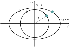
Figure 1: The configurations of two gravitons.

The organization of this paper is as follows: In section 2, by using the background field method around the setup mentioned above, we compute the functional determinants. Before performing the path integral for the fluctuations, it is necessary to take care of the time-dependence of the configuration of classical solutions. In section 3 the functional determinants are evaluated by expanding them with respect to the infinitesimal parameter $\epsilon$ . The evaluation is too complicated, and so we use the Mathematica [32]. The resulting effective action gives rise to the $1/r^{7}$-type potential as the leading term. Section 4 is devoted to a conclusion and discussions.

2 Two-Body Interaction of Point-Like Gravitons

From now on, let us examine the interaction potential between the point-like gravitons by using the setup proposed in Fig. 1. We will use the background field method as usual. Then the matrix fields are decomposed into backgrounds and fluctuations as follows:

$$X^{I}=B^{I}+Y^{I}\,,\quad\Theta=0+\Psi\,.$$ (2.1)

Here $B^{I}$ are classical backgrounds while $Y^{I}$ and $\Psi$ are quantum fluctuations around them. The fermionic background is taken to be zero.

The background for the configuration in Fig. 1 is described by the following $2\times 2$ matrices:

$$B^{I}=\begin{pmatrix}B^{I}_{(1)}&0\\ 0&B^{I}_{(2)}\end{pmatrix}\qquad(I=1,\ldots,9)\,,$$

$$B^{1}_{(1)}=r_{1}\cos\left(\frac{\mu}{3}t\right)\,,\qquad B^{2}_{(1)}=r_{1}\sin\left(\frac{\mu}{3}t\right)\,,$$

$$B^{1}_{(2)}=(r_{2}+\epsilon)\cos\left(\frac{\mu}{3}t\right)\,,\qquad B^{2}_{(2)}=(r_{2}-\epsilon)\sin\left(\frac{\mu}{3}t\right)$$

$$B^{3}_{(s)}=B^{a}_{(s)}=0\qquad(s=1,2~{};~{}a=4,\ldots,9)\,.$$ (2.2)

Two gravitons rotating in the 1-2 plane are diagonally embedded. Each of the gravitons carries a unit of the light-cone momentum and it is represented by a $1\times 1$ matrix. One of them rotates with a constant radius $r_{1}$ and the other one rotates elliptically with $r_{2}\pm\epsilon$ .

In order to perform the path integral for the fluctuations, we need to fix the gauge symmetry. In the matrix model computation, it is convenient to choose the background field gauge,

$$D_{\mu}^{\rm bg}A^{\mu}_{\rm qu}\equiv D_{t}A+i[B^{I},X^{I}]=0\,.$$ (2.3)

Then the corresponding gauge-fixing $S_{\mathrm{GF}}$ and Faddeev-Popov ghost $S_{\mathrm{FP}}$ terms are given by

$$S_{\mathrm{GF}}+S_{\mathrm{FP}}=\int\!dt\,{\rm Tr}\left(-\frac{1}{2}(D_{\mu}^{\rm bg}A^{\mu}_{\rm qu})^{2}-\bar{C}\partial_{t}D_{t}C+[B^{I},\bar{C}][X^{I},\,C]\right)\,.$$ (2.4)

Now, by inserting the decomposition of the matrix fields (2.1) into the matrix model action, we get the gauge fixed plane-wave action $S$ $(\equiv S_{\rm pp}+S_{\mathrm{GF}}+S_{\mathrm{FP}})$ expanded around the background. The resulting action is read as $S=S_{0}+S_{2}+S_{3}+S_{4}$ , where $S_{n}$ represents the action of order $n$ with respect to the quantum fluctuations and, for each $n$, its expression is

$$S_{0}=\int dt\,\mathrm{Tr}\bigg{[}\, \frac{1}{2}(\dot{B}^{I})^{2}-\frac{1}{2}\left(\frac{\mu}{3}\right)^{2}(B^{i})^{2}-\frac{1}{2}\left(\frac{\mu}{6}\right)^{2}(B^{a})^{2}+\frac{1}{4}([B^{I},\,B^{J}])^{2}-i\frac{\mu}{3}\epsilon^{ijk}B^{i}B^{j}B^{k}\bigg{]}~{},$$

$$S_{2}=\int dt\,\mathrm{Tr}\bigg{[}\, \frac{1}{2}(\dot{Y}^{I})^{2}-2i\dot{B}^{I}[A,\,Y^{I}]+\frac{1}{2}([B^{I},\,Y^{J}])^{2}+[B^{I},\,B^{J}][Y^{I},\,Y^{J}]-i\mu\epsilon^{ijk}B^{i}Y^{j}Y^{k}$$

$$-\frac{1}{2}\left(\frac{\mu}{3}\right)^{2}(Y^{i})^{2}-\frac{1}{2}\left(\frac{\mu}{6}\right)^{2}(Y^{a})^{2}+i\Psi^{\dagger}\dot{\Psi}-\Psi^{\dagger}\gamma^{I}[\Psi,\,B^{I}]-i\frac{\mu}{4}\Psi^{\dagger}\gamma^{123}\Psi$$

$$-\frac{1}{2}\dot{A}^{2}-\frac{1}{2}([B^{I},\,A])^{2}+\dot{\bar{C}}\dot{C}+[B^{I},\,\bar{C}][B^{I},\,C]\,\bigg{]}~{},$$

$$S_{3}=\int dt\,\mathrm{Tr}\bigg{[} -i\dot{Y}^{I}[A,\,Y^{I}]-[A,\,B^{I}][A,\,Y^{I}]+[B^{I},\,Y^{J}][Y^{I},\,Y^{J}]+\Psi^{\dagger}[A,\,\Psi]$$

$$-\Psi^{\dagger}\gamma^{I}[\Psi,\,Y^{I}]-i\frac{\mu}{3}\epsilon^{ijk}Y^{i}Y^{j}Y^{k}-i\dot{\bar{C}}[A,\,C]+[B^{I},\,\bar{C}][Y^{I},\,C]\,\bigg{]}~{},$$

$$S_{4}=\int dt\,\mathrm{Tr}\bigg{[} -\frac{1}{2}([A,\,Y^{I}])^{2}+\frac{1}{4}([Y^{I},\,Y^{J}])^{2}\bigg{]}~{}.$$ (2.5)

Here the action of the first order becomes zero by using the equations of motion.

For the justification of one-loop computation or the semi-classical analysis, it should be made clear that $S_{3}$ and $S_{4}$ can be regarded as perturbations. For this purpose, following [8], we rescale the fluctuations and parameters as

$$A\rightarrow\mu^{-1/2}A\,,\quad Y^{I}\rightarrow\mu^{-1/2}Y^{I}\,,\quad C\rightarrow\mu^{-1/2}C\,,\quad\bar{C}\rightarrow\mu^{-1/2}\bar{C}\,,$$

$$r_{1,2}\rightarrow\mu r_{1,2}\,,\quad\epsilon\rightarrow\mu\epsilon\,,\quad t\rightarrow\mu^{-1}t\,.$$ (2.6)

Under this rescaling, the action $S$ becomes

$$S=S_{2}+\mu^{-3/2}S_{3}+\mu^{-3}S_{4}\,,$$ (2.7)

where the parameter $\mu$ in $S_{2}$, $S_{3}$ and $S_{4}$ has been replaced by 1 and so those do not have $\mu$ dependence. Now it is obvious that, in the large $\mu$ limit, $S_{3}$ and $S_{4}$ can be treated as perturbations and the one-loop computation gives the sensible result. Note that the analysis in the $S_{2}$ part is exact in the $\mu\rightarrow\infty$ limit.

Based on the structure of the classical background, we now take the quantum fluctuations in the $2\times 2$ off-diagonal matrices:

$$A=\begin{pmatrix}0&\Phi^{0}\\ \Phi^{0\dagger}&0\end{pmatrix}\,,\quad Y^{I}=\begin{pmatrix}0&\Phi^{I}\\ \Phi^{I\dagger}&0\end{pmatrix}\,,\quad\Psi=\begin{pmatrix}0&\chi\\ \chi^{\dagger}&0\\ \end{pmatrix}\,,$$

$$C=\begin{pmatrix}0&C\\ C^{\dagger}&0\end{pmatrix}\,,\quad\bar{C}=\begin{pmatrix}0&\bar{C}\\ \bar{C}^{\dagger}&0\end{pmatrix}\,.$$ (2.8)

Here we are interested in the interaction between the gravitons and so we set the diagonal components to zero. It is an easy task to show the quantum stability of each of the gravitons by following the method in [25, 29].

It is convenient to introduce the following quantities:

$$r\equiv r_{2}-r_{1}\,,\qquad g(t)=\epsilon^{2}+2\epsilon r\cos\left(\frac{2}{3}t\right)\,,\quad G_{m}\equiv\frac{1}{\partial_{t}^{2}+r^{2}+m^{2}}\,.$$ (2.9)

Here $G_{m}$ is a propagator for a mass $m$ . By using them we can express the functional determinants after the path integral in simpler forms. We will perform the path integral below for each of the parts, bosons, ghosts and fermions.

2.1 Boson Fluctuation

Let us first consider the bosonic parts. The Lagrangian $L_{\rm B}$ is composed of two parts:

$$L_{\rm B} = L_{SO(3)}+L_{SO(6)}\,,$$ (2.10)

$$L_{SO(3)} = -|\dot{\Phi}^{0}|^{2}+\left(r^{2}+g(t)\right)|\Phi^{0}|^{2}+|\dot{\Phi}^{i}|^{2}-(r^{2}+g(t))|\Phi^{i}|^{2}-\frac{1}{3^{2}}|\Phi^{i}|^{2}$$

$$+\frac{2}{3}i(r+\epsilon)\sin\left(\frac{t}{3}\right)(\Phi^{0\dagger}\Phi^{1}-\Phi^{1\dagger}\Phi^{0})-\frac{2}{3}i(r-\epsilon)\cos\left(\frac{t}{3}\right)\left(\Phi^{0\dagger}\Phi^{2}-\Phi^{2\dagger}\Phi^{0}\right)$$

$$-i(r+\epsilon)\cos\left(\frac{t}{3}\right)(\Phi^{2\dagger}\Phi^{3}-\Phi^{3\dagger}\Phi^{2})-i(r-\epsilon)\sin\left(\frac{t}{3}\right)(\Phi^{3\dagger}\Phi^{1}-\Phi^{1\dagger}\Phi^{3})\,,$$

$$L_{SO(6)} = |\dot{\Phi}^{a}|^{2}-(r^{2}+g(t))|\Phi^{a}|^{2}-\frac{1}{6^{2}}|\Phi^{a}|^{2}\,.$$ (2.12)

Here the gauge field is included in $L_{SO(3)}$ . The next task is to evaluate each of the parts.

SO(3) part

Now we shall consider the $SO(3)$ part. In the Lagrangian for the $SO(3)$ part, the four variables $\Phi^{0}$ , $\Phi^{i}$ $(i=1,2,3)$ are contained. The analysis of this part is complicated since these are coupled. In order to carry out the path integral, it is convenient to decouple the variables as much as possible. For this purpose we first take the coordinate transformation

$$\Phi^{1}\equiv\cos\left(\frac{t}{3}\right)\Phi^{r}-\sin\left(\frac{t}{3}\right)\Phi^{\theta}\,,\quad\Phi^{2}\equiv\sin\left(\frac{t}{3}\right)\Phi^{r}+\cos\left(\frac{t}{3}\right)\Phi^{\theta}\,,$$ (2.13)

and introduce the new variables $\Phi^{r}$ and $\Phi^{\theta}$ instead of $\Phi^{1}$ and $\Phi^{2}$ . The Lagrangian after the transformation is rewritten as

$$L_{SO(3)} = -|\dot{\Phi}^{0}|^{2}+(r^{2}+g(t))|\Phi^{0}|^{2}+|\dot{\Phi}^{r}|^{2}-(r^{2}+g(t))|\Phi^{r}|^{2}+|\dot{\Phi}^{\theta}|^{2}-(r^{2}+g(t))|\Phi^{\theta}|^{2}$$ (2.14)

$$+|\dot{\Phi}^{3}|^{2}-(r^{2}+g(t)+(1/3^{2}))|\Phi^{3}|^{2}+\frac{2}{3}(\Phi^{r\dagger}\dot{\Phi}^{\theta}-\Phi^{\theta\dagger}\dot{\Phi}^{r})$$

$$+\frac{2}{3}i\epsilon\sin(2t/3)(\Phi^{0\dagger}\Phi^{r}-\Phi^{r\dagger}\Phi^{0})-\frac{2}{3}i(r-\epsilon\cos(2t/3))(\Phi^{0\dagger}\Phi^{\theta}-\Phi^{\theta\dagger}\Phi^{0})$$

$$+i\epsilon\sin(2t/3)(\Phi^{3\dagger}\Phi^{r}-\Phi^{r\dagger}\Phi^{3})+i(r+\epsilon\cos(2t/3))(\Phi^{3\dagger}\Phi^{\theta}-\Phi^{\theta\dagger}\Phi^{3})\,.$$

Taking the shift of $\Phi^{0}$ and $\Phi^{3}$ defined by

$$\Phi^{0}\equiv\Phi^{0}{}^{\prime}-\frac{2}{3}i(G_{0}^{-1}+g(t))^{-1}\left[\epsilon\sin\left(\frac{2}{3}t\right)\Phi^{r}-(r-\epsilon\cos\left(\frac{2}{3}t\right))\Phi^{\theta}\right]\,,$$

$$\Phi^{3}\equiv\Phi^{3}{}^{\prime}+i(G_{1/3}^{-1}+g(t))^{-1}\left[\epsilon\sin\left(\frac{2}{3}t\right)\Phi^{r}+(r+\epsilon\cos\left(\frac{2}{3}t\right))\Phi^{\theta}\right]\,,$$

we obtain the following Lagrangian:

$$L_{SO(3)}=\Phi^{0}{}^{\prime}{}^{\dagger}(G_{0}^{-1}+g(t))\Phi^{0}{}^{\prime}-\Phi^{3}{}^{\prime}{}^{\dagger}(G_{1/3}^{-1}+g(t))\Phi^{3}{}^{\prime}-\Phi^{r\dagger}(G_{0}^{-1}+g(t))\Phi^{r}$$

$$-\Phi^{\theta\dagger}(G_{0}^{-1}+g(t))\Phi^{\theta}+\frac{2}{3}\Phi^{r\dagger}\dot{\Phi}^{\theta}-\frac{2}{3}\Phi^{\theta\dagger}\dot{\Phi}^{r}$$ (2.15)

$$-\Phi^{r\dagger}\left\{\epsilon^{2}\sin\left(2t/3\right)\left[\frac{4}{9}(G_{0}^{-1}+g(t))^{-1}-(G_{1/3}^{-1}+g(t))^{-1}\right]\sin\left(2t/3\right)\right\}\Phi^{r}$$

$$-\Phi^{\theta\dagger}\left\{\left(r-\epsilon\cos\left(2t/3\right)\right)\left[\frac{4}{9}(G_{0}^{-1}+g(t))^{-1}-(G_{1/3}^{-1}+g(t))^{-1}\right]\left(r-\epsilon\cos\left(2t/3\right)\right)\right\}\Phi^{\theta}$$

$$+\Phi^{\theta\dagger}\left\{\left(r-\epsilon\cos\left(2t/3\right)\right)\left[\frac{4}{9}(G_{0}^{-1}+g(t))^{-1}+(G_{1/3}^{-1}+g(t))^{-1}\right]\epsilon\sin(2t/3)\right\}\Phi^{r}$$

$$+\Phi^{r\dagger}\left\{\epsilon\sin\left(2t/3\right)\left[\frac{4}{9}(G_{0}^{-1}+g(t))^{-1}+(G_{1/3}^{-1}+g(t))^{-1}\right]\left(r-\epsilon\cos\left(2t/3\right)\right)\right\}\Phi^{\theta}\,.$$

Note that $\Phi^{0}$ and $\Phi^{3}$ are decoupled from $\Phi^{r}$ and $\Phi^{\theta}$ at this stage, but $\Phi^{r}$ and $\Phi^{\theta}$ are still coupled. We can however perform the path integral for $\Phi^{r}$ and $\Phi^{\theta}$ by using the formula

$$\begin{pmatrix}A&B\\ C&D\end{pmatrix}=\begin{pmatrix}A&0\\ C&1\end{pmatrix}\begin{pmatrix}1&A^{-1}B\\ 0&D-CA^{-1}B\end{pmatrix}\,.$$ (2.16)

The resulting effective action for the $SO(3)$ part is given by

$${\rm e}^{i\Gamma_{SO(3)}}=\left[\det(G_{0}^{-1}+g(t))\cdot\det(G_{1/3}^{-1}+g(t))\cdot\det A\cdot\det(D-CA^{-1}B)\right]^{-1}\,,$$ (2.17)

$$A=G_{0}^{-1}+g(t)+\epsilon^{2}\sin\left(2t/3\right)\left[\frac{4}{9}\,\frac{1}{G_{0}^{-1}+g(t)}-\frac{1}{G_{1/3}^{-1}+g(t)}\right]\sin\left(2t/3\right)\,,$$

$$D=G_{0}^{-1}+g(t)+\frac{4}{9}\left(r-\epsilon\cos\left(2t/3\right)\right)\frac{1}{G_{0}^{-1}+g(t)}\left(r-\epsilon\cos\left(2t/3\right)\right)$$

$$\qquad\qquad-\left(r+\epsilon\cos\left(2t/3\right)\right)\frac{1}{G_{1/3}^{-1}+g(t)}\left(r+\epsilon\cos\left(2t/3\right)\right)\,,$$

$$B=-\frac{2}{3}\partial_{t}-\frac{4}{9}\epsilon\sin\left(2t/3\right)\frac{1}{G_{0}^{-1}+g(t)}\left(r-\epsilon\cos\left(2t/3\right)\right)$$

$$\qquad\qquad-\epsilon\sin\left(2t/3\right)\frac{1}{G_{1/3}^{-1}+g(t)}\left(r+\epsilon\cos\left(2t/3\right)\right)\,,$$

$$C=\frac{2}{3}\partial_{t}-\frac{4}{9}\left(r-\epsilon\cos\left(2t/3\right)\right)\frac{1}{G_{0}^{-1}+g(t)}\epsilon\sin(2t/3)$$

$$\qquad\qquad-\left(r+\epsilon\cos\left(2t/3\right)\right)\frac{1}{G_{1/3}^{-1}+g(t)}\epsilon\sin(2t/3)\,.$$

Then we will examine the $SO(6)$ part.

SO(6) part

It is straightforward to perform the path integral for the $SO(6)$ part. The result is

$${\rm e}^{\Gamma_{SO(6)}}={\rm e}^{i\Gamma_{SO(6)}^{(0)}}(\det\left(1+G_{1/6}\,g(t)\right))^{-6}\,,$$ (2.18)

where the $\epsilon$-independent part is written as

$${\rm e}^{i\Gamma^{(0)}_{SO(6)}}=(\det G_{1/6}^{-1})^{-6}\,.$$ (2.19)

2.2 Ghost Fluctuation

Next we shall consider the ghost part. The Lagrangian for the ghost part is given by

$$L_{\rm G}=\dot{\bar{C}}\dot{C}^{\dagger}+\dot{\bar{C}}^{\dagger}\dot{C}-(r^{2}+g(t))(\bar{C}C^{\dagger}+\bar{C}^{\dagger}C)\,.$$ (2.20)

The path integral for (2.20) is immediately evaluated as

$$[\det\left(G_{0}^{-1}+g(t)\right)]^{2}\,.$$ (2.21)

2.3 Fermion Fluctuation

Finally, let us discuss the fermionic part. The Lagrangian for the fermion fluctuations is given by

$$L_{\rm F} = 2\Bigl{[}i\chi^{\dagger}\dot{\chi}-r\chi^{\dagger}\left(\gamma^{1}\cos\left(\frac{t}{3}\right)+\gamma^{2}\sin\left(\frac{t}{3}\right)\right)\chi$$ (2.22)

$$-\epsilon\chi^{\dagger}\left(\gamma^{1}\cos\left(\frac{t}{3}\right)-\gamma^{2}\sin\left(\frac{t}{3}\right)\right)\chi-\frac{i}{4}\chi^{\dagger}\gamma^{123}\chi\Bigr{]}\,.$$

Then we decompose the spinor $\chi$ into two components as follows:

$$\chi=\dbinom{\chi_{A\alpha}}{\hat{\chi}_{\alpha}^{A}}\,,\qquad\hat{\chi}_{\alpha}^{A}\equiv\epsilon_{\alpha\beta}\hat{\chi}^{A\beta}\,.$$ (2.23)

According to this decomposition, the $SO(9)$ gamma matrices should also be decomposed. In our analysis only $\gamma^{1}$ , $\gamma^{2}$ and $\gamma^{3}$ are necessary and hence we write down only them here,

$$\gamma^{i}=\begin{pmatrix}-\sigma^{i}\times 1&0\\ 0&\sigma^{i}\times 1\\ \end{pmatrix}\qquad(i=1,2,3)\,.$$ (2.24)

For the detail of the decomposition of the gamma matrices, see [8, 25]. The Lagrangian after the decomposition is written as

$$L_{\rm F} = i\chi^{\dagger A\alpha}\dot{\chi}_{A\alpha}-\frac{1}{4}\chi^{\dagger A\alpha}\chi_{A\alpha}+i\hat{\chi}^{\dagger\alpha}_{A}\dot{\hat{\chi}}_{\alpha}^{A}+\frac{1}{4}\hat{\chi}^{\dagger\alpha}_{A}\hat{\chi}_{\alpha}^{A}$$

$$+\chi^{\dagger A\alpha}\left[(r+\epsilon)\cos(t/3)\cdot\sigma^{1}+(r-\epsilon)\sin(t/3)\cdot\sigma^{2}\,\right]_{\alpha}^{~{}\beta}\chi_{A\beta}$$

$$-\hat{\chi}^{\dagger\alpha}_{A}\left[(r+\epsilon)\cos(t/3)\cdot\sigma^{1}+(r-\epsilon)\sin(t/3)\cdot\sigma^{2}\,\right]_{\alpha}^{~{}\beta}\hat{\chi}_{\beta}^{A}\,.$$

Here it is convenient to introduce new spinors $\chi^{\prime}$ and $\tilde{\chi}$ defined by

$$\chi_{A\alpha}=({\rm e}^{-i\sigma^{3}\frac{t}{6}})_{\alpha}^{~{}\beta}\,\chi^{\prime}_{A\beta}\,,\qquad\hat{\chi}=({\rm e}^{-i\sigma^{3}\frac{t}{6}})_{\alpha}^{~{}\beta}\,\tilde{\chi}_{\beta}^{A}\,.$$ (2.26)

By using the formulae:

$${\rm e}^{i\sigma^{3}\frac{t}{6}}\left[\sigma^{1}\cos(t/3)+\sigma^{2}\sin(t/3)\right]{\rm e}^{-i\sigma^{3}\frac{t}{6}}=\sigma^{1}\,,$$

$${\rm e}^{i\sigma^{3}\frac{t}{6}}\left[\sigma^{1}\cos(t/3)-\sigma^{2}\sin(t/3)\right]{\rm e}^{-i\sigma^{3}\frac{t}{6}}=\sigma^{1}\cos(2t/3)-\sigma^{2}\sin(2t/3)\,,$$ (2.27)

we can rewrite the Lagrangian as

$$L_{\rm F} = i\chi^{\prime}{}^{\dagger A\alpha}\dot{\chi}^{\prime}_{A\alpha}-\frac{1}{4}\chi^{\prime}{}^{\dagger A\alpha}\chi^{\prime}_{A\alpha}+\frac{1}{6}\chi^{\prime}{\dagger A\alpha}(\sigma^{3})_{\alpha}^{~{}\beta}\chi^{\prime}_{A\beta}+i\tilde{\chi}^{\dagger\alpha}_{A}\dot{\tilde{\chi}}_{\alpha}^{A}+\frac{1}{4}\tilde{\chi}^{\dagger\alpha}_{A}\tilde{\chi}_{\alpha}^{A}+\frac{1}{6}\tilde{\chi}^{\dagger A\alpha}(\sigma^{3})_{\alpha}^{~{}\beta}\tilde{\chi}_{A\beta}$$

$$+\chi^{\prime}{}^{\dagger A\alpha}\left[\sigma^{1}(r+\epsilon\cos(2t/3))-\sigma^{2}\epsilon\sin(2t/3)\right]_{\alpha}^{~{}\beta}\chi^{\prime}_{A\beta}$$

$$-\tilde{\chi}^{\dagger\alpha}_{A}\left[\sigma^{1}(r+\epsilon\cos(2t/3))-\sigma^{2}\epsilon\sin(2t/3)\right]_{\alpha}^{~{}\beta}\tilde{\chi}^{A}_{\beta}\,.$$

Then we express the two components of the spinors $\chi^{\prime}$ and $\tilde{\chi}$ as

$$\chi^{\prime}=(\pi,\eta)\,,\qquad\tilde{\chi}=(\tilde{\pi},\tilde{\eta})\,.$$ (2.28)

When the Lagrangian is described in terms of $\pi,~{}\eta,~{}\tilde{\pi},$ and $\tilde{\eta}$ , it is decomposed into two parts: $(\pi,\eta)$-system and $(\tilde{\pi},\tilde{\eta})$-system. The Lagrangian for each of these system are given by

$$L_{\rm F} = L_{\pi,\eta}+L_{\tilde{\pi},\tilde{\eta}}\,,$$ (2.29)

$$L_{\pi,\eta} = i\pi^{\dagger}\dot{\pi}-\frac{1}{12}\pi^{\dagger}\pi+i\eta^{\dagger}\dot{\eta}-\frac{5}{12}\eta^{\dagger}\eta$$ (2.30)

$$+(r+\epsilon{\rm e}^{\frac{2}{3}it})\pi^{\dagger}\eta+(r+\epsilon{\rm e}^{-\frac{2}{3}it})\eta^{\dagger}\pi\,,$$

$$L_{\tilde{\pi},\tilde{\eta}} = i\tilde{\pi}^{\dagger}\dot{\tilde{\pi}}+\frac{5}{12}\tilde{\pi}^{\dagger}\tilde{\pi}+i\tilde{\eta}^{\dagger}\dot{\tilde{\eta}}+\frac{1}{12}\tilde{\eta}^{\dagger}\tilde{\eta}$$ (2.31)

$$-(r+\epsilon{\rm e}^{\frac{2}{3}it})\tilde{\pi}^{\dagger}\tilde{\eta}-(r+\epsilon{\rm e}^{-\frac{2}{3}it})\tilde{\eta}^{\dagger}\tilde{\pi}\,.$$

By using the formula (2.16) , we can perform the path integral for $\pi$ , $\eta$ , $\tilde{\pi}$ and $\tilde{\eta}$ . The effective action is given by

$${\rm e}^{i\Gamma_{\rm F}}=\det\left[(i\partial_{t}-\frac{1}{12})(i\partial_{t}-\frac{5}{12})-r^{2}\right]^{4}\det\left[1-\frac{1}{(i\partial_{t}-\frac{1}{12})(i\partial_{t}-\frac{5}{12})-r^{2}}E\right]^{4}\times$$

$$\quad\times\det\left[(i\partial_{t}+\frac{1}{12})(i\partial_{t}+\frac{5}{12})-r^{2}\right]^{4}\det\left[1-\frac{1}{(i\partial_{t}+\frac{1}{12})(i\partial_{t}+\frac{5}{12})-r^{2}}\tilde{E}\right]^{4}\,,$$ (2.32)

where $E$ and $\tilde{E}$ are defined by, respectively,

$$E=r\epsilon{\rm e}^{\frac{2}{3}it}+(i\partial_{t}-\frac{1}{12})\epsilon{\rm e}^{-\frac{2}{3}it}\frac{1}{i\partial_{t}-\frac{1}{12}}(r+\epsilon{\rm e}^{\frac{2}{3}it})\,,$$

$$\tilde{E}=r\epsilon{\rm e}^{\frac{2}{3}it}+(i\partial_{t}+\frac{5}{12})\epsilon{\rm e}^{-\frac{2}{3}it}\frac{1}{i\partial_{t}+\frac{5}{12}}(r+\epsilon{\rm e}^{\frac{2}{3}it})\,.$$ (2.33)

Now we have finished the path integration for the fluctuations. The remaining task is to evaluate the functional determinant. This will be discussed in the next section.

3 Effective Action

From now on we evaluate the determinant factors obtained in the previous section. In the evaluation we use the formula,

$$\det(1+\epsilon g)=\exp\left(\epsilon{\rm tr}g-\frac{1}{2}\epsilon^{2}{\rm tr}g^{2}+\cdots\right)\,,$$

and therefore the resulting effective action is expressed as an expansion in terms of $\epsilon$ ,

$$\Gamma_{\rm eff}=\Gamma^{(0)}_{\rm eff}+\epsilon^{2}\Gamma^{(2)}_{\rm eff}+\epsilon^{4}\Gamma^{(4)}_{\rm eff}+\mathcal{O}(\epsilon^{6})\,,$$ (3.1)

where the terms of order $\epsilon^{n}$ with odd $n$ are absent in our computation in accordance with the logic of our previous work [29].

Before going to the analysis of the $\epsilon$-dependent part, let us consider the $\epsilon$-independent part $\Gamma^{(0)}_{\rm eff}$ and show the one-loop flatness:

$$\Gamma^{(0)}_{\rm eff}=0\,.$$

3.1 One-Loop Flatness

For the $SO(3)$ part, the effective action is

$${\rm e}^{i\Gamma_{SO(3)}}=\left[\det(G_{0}^{-1})\cdot\det(G_{1/3}^{-1})\cdot\det A\cdot\det(D-CA^{-1}B)\right]^{-1}\,,$$ (3.2)

where the components $A,B,C$ and $D$ are given by

$$A=G_{0}^{-1}\,,\quad B=-\frac{2}{3}\partial_{t}\,,\quad C=\frac{2}{3}\partial_{t}\quad D=G_{0}^{-1}+\frac{4}{9}r^{2}G_{0}-r^{2}G_{1/3}\,.$$ (3.3)

Then we obtain that

$$D-CA^{-1}B=\partial_{t}^{2}+r^{2}+\frac{4}{9}-\frac{r^{2}}{\partial_{t}^{2}+r^{2}+\frac{1}{9}}\,.$$ (3.4)

Hence we can rewrite a part of the determinant factors as follows:

$$\det(G_{1/3}^{-1})\cdot\det(D-CA^{-1}B)=\det\left[\left(\partial_{t}^{2}+r^{2}+\frac{4}{9}\right)\left(\partial_{t}^{2}+r^{2}+\frac{1}{9}\right)-r^{2}\right]$$

$$= \det\left[\partial_{t}^{2}+\left(\partial_{t}^{2}+r^{2}-\frac{2}{9}\right)^{2}\right]=\det\left[\left(\partial_{t}^{2}+i\partial_{t}+r^{2}-\frac{2}{9}\right)\left(\partial_{t}^{2}-i\partial_{t}+r^{2}-\frac{2}{9}\right)\right]\,.$$

By using the formula

$$\int^{\infty}_{-\infty}\frac{dk}{2\pi}\,\ln(-k^{2}+2pk+m^{2}-i\epsilon)=i\sqrt{m^{2}+p^{2}}\,,$$ (3.5)

the contribution to the effective action is evaluated as

$$2\sqrt{r^{2}+\frac{1}{36}}\,.$$

This includes the only contribution from the physical degrees of freedom and the unphysical mode related to the gauge field is surely canceled out with the ghost contribution.

Turning to the $SO(6)$ part, we see that the contribution from the $SO(6)$ part is given by

$$6\sqrt{r^{2}+\frac{1}{36}}\,.$$

Hence the total bosonic contribution is

$$\Gamma^{(0)}_{\rm B}=8\sqrt{r^{2}+\frac{1}{36}}\,.$$ (3.6)

Finally, let us examine the fermionic contribution. The effective action is given by

$${\rm e}^{i\Gamma_{\rm F}}=\det\left[\left(i\partial_{t}-\frac{1}{12}\right)\left(i\partial_{t}-\frac{5}{12}\right)-r^{2}\right]^{4}\cdot\det\left[\left(i\partial_{t}+\frac{1}{12}\right)\left(i\partial_{t}+\frac{5}{12}\right)-r^{2}\right]^{4}$$ (3.7)

Here, noting that

$$\left(i\partial_{t}-\frac{5}{12}\right)-r^{2}=-\left(\partial_{t}^{2}+\frac{1}{2}i\partial_{t}-\frac{5}{144}\right)\,,$$

the total fermionic contribution is evaluated as

$$\Gamma^{(0)}_{\rm F}=-8\sqrt{r^{2}+\frac{1}{36}}\,.$$ (3.8)

Therefore the total contribution from the $\epsilon$-dependent parts becomes zero:

$$\Gamma^{(0)}_{\rm eff} = \Gamma^{(0)}_{\rm B}+\Gamma^{(0)}_{\rm F}$$

$$= 8\sqrt{r^{2}+\frac{1}{36}}-8\sqrt{r^{2}+\frac{1}{36}}=0\,.$$

Thus, the one-loop flatness:

$$\Gamma^{(0)}_{\rm eff}=0\,,$$ (3.9)

has been shown in our setup.

3.2 Evaluation of $\epsilon$-Dependent Part

The evaluation of the $\epsilon$-dependent parts is quite complicated and hence we need to use the Mathematica [32]. Here we shall show only the results after evaluating the functional traces. We note that, due to the enormous complexity of computation, the results are obtained in the large-distance expansion, $r\gg 1$.

First of all, at $\epsilon^{2}$ order, we obtain

$$\Gamma^{(2)}_{\rm B} =-\Gamma^{(2)}_{\rm F}$$

$$=-\int dt\left(\frac{2}{r}+\frac{17}{2^{2}\cdot 3^{2}}\frac{1}{r^{3}}+\frac{61}{2^{6}\cdot 3^{3}}\frac{1}{r^{5}}+\frac{1129}{2^{9}\cdot 3^{6}}\frac{1}{r^{7}}+\frac{26891}{2^{14}\cdot 3^{8}}\frac{1}{r^{9}}\right)+\mathcal{O}(r^{-11})\,.$$ (3.10)

We can see the cancellation between contributions of bosons and fermions up to the $1/r^{9}$ order. It is, however, possible to show that the cancellation is exact from the numerical analysis. Hence we have shown that the effective action with $\epsilon^{2}$ order should vanish:

$$\Gamma^{(2)}_{\rm eff}=0\,.$$ (3.11)

Now let us see the effective action at $\epsilon^{4}$ order. The contribution from the physical modes in the $SO(3)$ part is given by

$$\widehat{\Gamma}^{(4)}_{SO(3)}=\int dt\left(-\frac{1}{2^{5}}\frac{1}{r^{3}}-\frac{883}{2^{8}\cdot 3}\frac{1}{r^{5}}+\frac{11\cdot 19\cdot 443}{2^{12}\cdot 3^{3}}\frac{1}{r^{7}}+\frac{11\cdot 29\cdot 28793}{2^{15}\cdot 3^{6}}\frac{1}{r^{9}}\right)+\mathcal{O}(r^{-11})\,,$$ (3.12)

and, for the $SO(6)$ part, the contribution is

$$\Gamma^{(4)}_{SO(6)}=\int dt\left(-\frac{3}{2^{5}}\frac{1}{r^{3}}+\frac{77}{2^{8}}\frac{1}{r^{5}}+\frac{19\cdot 131}{2^{12}\cdot 3}\frac{1}{r^{7}}+\frac{13^{2}\cdot 4271}{2^{15}\cdot 3^{5}}\frac{1}{r^{9}}\right)+\mathcal{O}(r^{-11})\,.$$ (3.13)

Hence the total contribution of the bosonic parts is

$$\Gamma^{(4)}_{\rm B} =\widehat{\Gamma}^{(4)}_{SO(3)}+\Gamma^{(4)}_{SO(6)}$$

$$=\int dt\left(-\frac{1}{2^{3}}\frac{1}{r^{3}}-\frac{163}{2^{6}\cdot 3}\frac{1}{r^{5}}+\frac{17\cdot 19\cdot 89}{2^{10}\cdot 3^{3}}\frac{1}{r^{7}}+\frac{131\cdot 21661}{2^{13}\cdot 3^{6}}\frac{1}{r^{9}}\right)+\mathcal{O}(r^{-11})\,.$$ (3.14)

The contribution of the fermions is totally represented by

$$\Gamma^{(4)}_{\rm F}=\int dt\left(\frac{1}{2^{3}}\frac{1}{r^{3}}+\frac{163}{2^{6}\cdot 3}\frac{1}{r^{5}}+\frac{71\cdot 163}{2^{10}\cdot 3^{3}}\frac{1}{r^{7}}+\frac{773\cdot 1493}{2^{13}\cdot 3^{6}}\frac{1}{r^{9}}\right)+\mathcal{O}(r^{-11})\,.$$ (3.15)

Thus the net effective action at $\epsilon^{4}$ order is given by

$$\Gamma^{(4)}_{\rm eff} =\Gamma^{(4)}_{\rm B}+\Gamma^{(4)}_{\rm F}$$

$$=\int dt\left(\,\frac{35}{24}\frac{1}{r^{7}}+\frac{385}{576}\frac{1}{r^{9}}\,\right)+\mathcal{O}(r^{-11})\,.$$ (3.16)

The contributions of the parts with $1/r$ , $1/r^{3}$ and $1/r^{5}$ are exactly canceled out. These cancellations would be basically due to the supersymmetries. And the resulting effective potential is $1/r^{7}$-type as in the case of the BFSS matrix model. We should note that the above expression is written in the Minkowski formulation and so the leading term of the potential is attractive. Then we should note that the subleading term of order $1/r^{9}$ exists and it is also attractive. Firstly, the term of $1/r^{9}$-type does not appear in the BFSS case where the subleading term is $1/r^{11}$ and this corresponds to the dipole-dipole interaction . The presence of the $1/r^{9}$ term implies the existence of the dipole-graviton interaction or the interaction between single poles. The appearance of this term is a new effect intrinsic to the pp-wave case. Furthermore, we should note that the subleading term is attractive while the subleading term in the spherical membrane cases is repulsive. Since the transverse $SO(9)$ symmetry is broken due to the effect of non-vanishing curvature of the pp-wave background, it is not a mystery to obtain the different graviton potential in each of the $SO(3)$ and $SO(6)$ symmetric spaces. It is, however, still interesting to see the apparent difference between the graviton interactions in the $SO(3)$ and the $SO(6)$ symmetric spaces.

4 Conclusion and Discussion

We have computed the two-body interaction potential between the point-like graviton solutions in a sub-plane in the $SO(3)$ symmetric space by considering the configuration drawn in Fig.1. The leading term of the potential is $1/r^{7}$ and thus strongly suggests that our result should be closely related to the scattering in the light-front eleven-dimensional supergravity. We expect that this potential should be realized from the computation in the supergravity side by using the spectrum of the linearized supergravity around the pp-wave background [31]. In this direction the work [33] would be helpful.

So far we have computed the interaction of the spherical membrane fuzzy spheres (giant gravitons) in the $SO(6)$ space and the scattering of the point-like gravitons in the $SO(3)$ symmetric space. It is interesting to consider the interaction between a point-like graviton and a spherical membrane graviton. We hope that the result will be reported in the near future as another publication [34].

Our analysis and results will be an important clue to study some features of M-theory on the pp-wave background and to shed light on the substance of M-theory.

References

• [1] T. Banks, W. Fischler, S. H. Shenker and L. Susskind, “M theory as a matrix model: A conjecture,” Phys. Rev. D 55 (1997) 5112 [arXiv:hep-th/9610043].
• [2] N. Ishibashi, H. Kawai, Y. Kitazawa and A. Tsuchiya, “A large-N reduced model as superstring,” Nucl. Phys. B 498 (1997) 467 [arXiv:hep-th/9612115].
• [3] R. Dijkgraaf, E. Verlinde and H. Verlinde, “Matrix string theory,” Nucl. Phys. B 500 (1997) 43 [arXiv:hep-th/9703030].
• [4] E. Witten, “String theory dynamics in various dimensions,” Nucl. Phys. B 443 (1995) [arXiv:hep-th/9503124].
• [5] B. de Wit, J. Hoppe and H. Nicolai, “On the quantum mechanics of supermembranes,” Nucl. Phys. B 305 (1988) 545.
• [6] D. Berenstein, J. M. Maldacena and H. Nastase, “Strings in flat space and pp waves from N = 4 super Yang Mills,” JHEP 0204 (2002) 013 [arXiv:hep-th/0202021].
• [7] J. Kowalski-Glikman, “Vacuum states in supersymmetric Kaluza-Klein theory,” Phys. Lett. B 134 (1984) 194.
• [8] K. Dasgupta, M. M. Sheikh-Jabbari and M. Van Raamsdonk, “Matrix perturbation theory for M-theory on a PP-wave,” JHEP 0205 (2002) 056 [arXiv:hep-th/0205185].
• [9] K. Sugiyama and K. Yoshida, “Supermembrane on the pp-wave background,” Nucl. Phys. B 644 (2002) 113 [arXiv:hep-th/0206070]; “BPS conditions of supermembrane on the pp-wave,” Phys. Lett. B 546 (2002) 143 [arXiv:hep-th/0206132]; N. Nakayama, K. Sugiyama and K. Yoshida, “Ground state of the supermembrane on a pp-wave,” Phys. Rev. D 68 (2003) 026001, [arXiv:hep-th/0209081].
• [10] T. Banks, N. Seiberg and S. H. Shenker, “Branes from matrices,” Nucl. Phys. B 490 (1997) 91 [arXiv:hep-th/9612157].
• [11] S. Hyun and H. Shin, “Branes from matrix theory in pp-wave background,” Phys. Lett. B 543 (2002) 115, hep-th/0206090.
• [12] K. Sugiyama and K. Yoshida, “Type IIA string and matrix string on pp-wave,” Nucl. Phys. B 644 (2002) 128 [arXiv:hep-th/0208029].
• [13] S. Hyun and H. Shin, ‘$`\mathcal{N}$ = (4,4) type IIA string theory on pp-wave background,” JHEP 0210 (2002) 070 [arXiv:hep-th/0208074].
• [14] Y. Sekino and T. Yoneya, “From supermembrane to matrix string,” Nucl. Phys. B 619 (2001) 22 [arXiv:hep-th/0108176].
• [15] G. Bonelli, “Matrix strings in pp-wave backgrounds from deformed super Yang-Mills theory,” JHEP 0208 (2002) 022 [arXiv:hep-th/0205213].
• [16] R. C. Myers, “Dielectric-branes,” JHEP 9912 (1999) 022 [arXiv:hep-th/9910053].
• [17] K. Dasgupta, M. M. Sheikh-Jabbari and M. Van Raamsdonk, “Protected multiplets of M-theory on a plane wave,” JHEP 0209 (2002) 021 [arXiv:hep-th/0207050].
• [18] N. Kim and J. Plefka, “On the spectrum of pp-wave matrix theory,” Nucl. Phys. B 643 (2002) 31 [arXiv:hep-th/0207034].
• [19] N. Kim and J. H. Park, “Superalgebra for M-theory on a pp-wave,” Phys. Rev. D 66 (2002) 106007 [arXiv:hep-th/0207061].
• [20] J. Maldacena, M. M. Sheikh-Jabbari and M. Van Raamsdonk, “Transverse fivebranes in matrix theory,” JHEP 0301 (2003) 038 [arXiv:hep-th/0211139].
• [21] D. Bak, “Supersymmetric branes in PP wave background,” Phys. Rev. D 67 (2003) 045017, hep-th/0204033.
• [22] J. H. Park, “Supersymmetric objects in the M-theory on a pp-wave,” JHEP 0210 (2002) 032 [arXiv:hep-th/0208161].
• [23] D. Bak, S. Kim and K. Lee, “All higher genus BPS membranes in the plane wave background,” arXiv:hep-th/0501202.
• [24] K. Sugiyama and K. Yoshida, “Giant graviton and quantum stability in matrix model on PP-wave background,” Phys. Rev. D 66 (2002) 085022 [arXiv:hep-th/0207190].
• [25] H. Shin and K. Yoshida, “One-loop flatness of membrane fuzzy sphere interaction in plane-wave matrix model,” Nucl. Phys. B 679 (2004) 99 [arXiv:hep-th/0309258].
• [26] W. H. Huang, “Thermal instability of giant graviton in matrix model on pp-wave background,” Phys. Rev. D 69 (2004) 067701 [arXiv:hep-th/0310212].
• [27] H. Shin and K. Yoshida, “Thermodynamics of fuzzy spheres in pp-wave matrix model,” Nucl. Phys. B 701 (2004) 380 [arXiv:hep-th/0401014]; “Thermodynamic behavior of fuzzy membranes in PP-wave matrix model,” Phys. Lett. B 627 (2005) 188 [arXiv:hep-th/0507029].
• [28] K. Furuuchi, E. Schreiber and G. W. Semenoff, “Five-brane thermodynamics from the matrix model,” arXiv:hep-th/0310286,
G. W. Semenoff, “Matrix model thermodynamics,” arXiv:hep-th/0405107;
S. Hadizadeh, B. Ramadanovic, G. W. Semenoff and D. Young, “Free energy and phase transition of the matrix model on a plane-wave,” Phys. Rev. D 71 (2005) 065016 [arXiv:hep-th/0409318].
• [29] H. Shin and K. Yoshida, “Membrane fuzzy sphere dynamics in plane-wave matrix model,” Nucl. Phys. B 709 (2005) 69 [arXiv:hep-th/0409045].
• [30] D. Kabat and W. I. Taylor, “Spherical membranes in matrix theory,” Adv. Theor. Math. Phys. 2 (1998) 181 [arXiv:hep-th/9711078].
• [31] T. Kimura and K. Yoshida, “Spectrum of eleven-dimensional supergravity on a pp-wave background,” Phys. Rev. D 68 (2003) 125007 [arXiv:hep-th/0307193].
• [32] S. Wolfram, the Mathematica book, 4th edition (Cambridge, 1999).
• [33] H. K. Lee, T. McLoughlin and X. k. Wu, “Gauge / gravity duality for interactions of spherical membranes in 11-dimensional pp-wave,” Nucl. Phys. B 728 (2005) 1 [arXiv:hep-th/0409264].
• [34] H. Shin and K. Yoshida, in preparation.