CALT-68-2581

ITEP-TH-69/05

A nonlocal Poisson bracket of the sine-Gordon model



Andrei Mikhailov

California Institute of Technology 452-48, Pasadena CA 91125

and

Institute for Theoretical and Experimental Physics,
117259, Bol. Cheremushkinskaya, 25, Moscow, Russia

It is well known that the classical string on a two-sphere is more or less equivalent to the sine-Gordon model. We consider the nonabelian dual of the classical string on a two-sphere. We show that there is a projection map from the phase space of this model to the phase space of the sine-Gordon model. The corresponding Poisson structure of the sine-Gordon model is nonlocal with one integration.

1 Introduction.

The most well-known example of the AdS/CFT correspondence is the duality between the Type IIB superstring in $AdS_{5}\times S^{5}$ and the ${\cal N}=4$ supersymmetric Yang-Mills theory on ${\bf R}\times S^{3}$. At the level of the classical string we can consider a simpler example when the motion of the string is restricted to ${\bf R}\times S^{2}\subset AdS_{5}\times S^{5}$. The classical string on ${\bf R}\times S^{2}$ is essentially equivalent to a well-known integrable system, the sine-Gordon model [1]. But the symplectic structure of the classical string does not correspond to the canonical symplectic structure of the sine-Gordon model.

In this paper we will argue that the map from the classical string to the sine-Gordon can be understood as a kind of T-duality in $S^{2}$. We consider the infinite string on ${\bf R}\times S^{2}$. In Section 2 we introduce the classical field theory which is dual to the classical string on ${\bf R}\times S^{2}$. After imposing the Virasoro constraints the phase space becomes an affine bundle over the phase space of the sine-Gordon, modelled on the vector bundle of solutions of some auxiliary linear problem. The distribution of symplectic complements of the fibers is integrable. In Section 3 we explain how to restrict the symplectic form of the string to the integral manifold of this distribution and push it forward to the sine-Gordon phase space. This gives a nonlocal Poisson bracket of the sine-Gordon which is compatible with the standard Poisson bracket obtained from the sine-Gordon action. In Section 4 we return to the original system, the classical string on a sphere, and show that it leads to the same Poisson structure of the sine-Gordon model. This Poisson bracket and the corresponding symplectic form are given by Eqs. (36), (40) and (42).

This suggests that the quantization of the sigma-model on ${\bf R}\times S^{2}$ (after imposing the Virasoro constraints) could be closely related to the quantization of the sine-Gordon model with the nonlocal Poisson bracket.

A somewhat similar relation between the third Poisson structure of KdV and the WZNW model was obtained in [2]. The general theory of nonlocal Poisson brackets was developed in [3] and references therein. The importance of the non-standard Poisson brackets for AdS/CFT was emphasized in [4]. T-duality with respect to a nonabelian symmetry was discussed in [5, 6, 7, 8].

Note added in the revised version. Closely related results were previously obtained in [9]—[16], but from a different perspective. The main difference of our approach is that we start from the relativistic string and derive the Poisson brackets from the string worldsheet action. (While in [9]—[16] the Poisson brackets were essentially postulated.) The results of this work are extended to the superstring in $AdS_{5}\times S^{5}$ in [17].

2 T-dual of the classical string on a sphere.

The zero-curvature approach to the string on a sphere was suggested in the context of AdS/CFT in [18] and further developed in [19]. We start with the Lie algebra $\bf g$ and its subalgebra $\bf h$. Suppose that as a linear space ${\bf g}={\bf h}+{\bf j}$ where ${\bf j}={\bf h}^{\perp}$. Suppose that $[{\bf j},{\bf j}]\subset{\bf h}$. Consider a pair of the Lie algebra valued fields $J_{\pm},H_{\pm}$ such that $J_{\pm}\in{\bf j}$ and $H_{\pm}\in{\bf h}$. Consider the following zero curvature equations:

$$\left[\partial_{+}+H_{+}+{1\over z}J_{+},\partial_{-}+H_{-}+zJ_{-}\right]=0$$ (1)

In particular case when ${\bf g}=so(n+1)$ and ${\bf h}=so(n)$ the coset space is a sphere $S^{n}$ and the fields $H_{\pm}$ and $J_{\pm}$ have a very transparent geometrical meaning. Let us choose a local trivialization of the tangent bundle $TS^{n}$, that is specify at each point $x\in S^{n}$ a basis $e_{1}(x),\ldots,e_{n}(x)$ in the tangent space. Given the embedding of the classical string worldsheet $x(\tau,\sigma)$ we write

$$\partial_{\pm}x=\sum_{j=1}^{n}\phi^{j}_{\pm}e_{j}$$

We put

$$J_{\pm}=\left[\begin{array}[]{cccc}0&\phi^{1}_{\pm}&\ldots&\phi^{n}_{\pm}\\ -\phi^{1}_{\pm}&&&\\ \vdots&&0&\\ -\phi^{n}_{\pm}&&&\end{array}\right]$$

and define $H_{\pm}$ as an antisymmetric $n\times n$ matrix $H_{\pm}^{ij}$ such that

$$D_{\pm}e_{i}=e^{j}H_{\pm}^{ji}$$

Then equations (1) encode the string equations of motion

$$D_{+}\partial_{-}x=D_{-}\partial_{+}x=0$$

and the relation between the Riemann tensor and the metric tensor for the sphere:

$$R^{i}_{jkl}\partial_{+}x^{k}\partial_{-}x^{l}=\partial_{+}x^{i}\partial_{-}x^{j}-\partial_{-}x^{i}\partial_{+}x^{j}$$

Let us now consider a particular case when $n=3$, the target space is $S^{2}$. The point of the two-sphere is usually denoted ${\bf n}$: $x={\bf n}$. We can think of ${\bf n}$ as a unit vector in ${\bf R}^{3}$. Suppressing the vector index $i=1,2$ we can write:

$$\phi_{\pm}=\partial_{\pm}{\bf n}$$

If $\xi$ is a section of the restriction to the string worldsheet of the tangent bundle to the sphere, then we have

$$[D_{+},D_{-}]\xi=\phi_{+}(\phi_{-},\xi)-\phi_{-}(\phi_{+},\xi)$$ (2)

Define the operator $I$ on the tangent space as a rotation by $\pi\over 2$, so that $I^{2}=-1$. We will consider the classical field theory with the following action:

$$S=\int d\tau d\sigma\left\{\left(\phi_{+},(1-\psi I)\phi_{-}\right)+\right.$$

$$\left.+(\phi_{+},D_{-}\lambda)-(\phi_{-},D_{+}\lambda)+\psi(\partial_{+}A_{-}-\partial_{-}A_{+})\right\}$$ (3)

where $\lambda$ and $\psi$ are Lagrange multipliers and

$$D_{\pm}=\partial_{\pm}+IA_{\pm}$$

We conjecture that the quantum theory with the action (2) is equivalent to the string on $S^{2}$. We do not have a solid argument for this, but naively if we integrate out $\lambda$ and $\psi$ we return to the standard action $\int d\tau d\sigma(\phi_{+},\phi_{-})$ of the classical string on $S^{2}$. It is possible that the correct statement of quantum equivalence would require the supersymmetric extension of the model. We will now study the Poisson structure of the theory with the action (2) and then in Section 4 we will show that the standard action of the classical string $\int d\tau^{+}d\tau^{-}(\partial_{+}{\bf n},\partial_{-}{\bf n})$ leads to essentially the same Poisson structure.

The action (3) has a gauge symmetry corresponding to the change of the basis in the tangent space to $S^{2}$:

$$\delta\phi_{\pm}=\epsilon I.\phi_{\pm},\;\;\delta\lambda=\epsilon I.\lambda,\;\;\delta A_{\pm}=-\partial_{\pm}\epsilon,\;\;\delta\psi=0$$ (4)

The equations of motion are:

$$D_{-}\phi_{+}=D_{+}\phi_{-}=0$$ (5)

$$D_{-}\lambda=-(1-\psi I)\phi_{-}$$ (6)

$$D_{+}\lambda=(1+\psi I)\phi_{+}$$ (7)

$$\partial_{+}\psi=(\phi_{+},I.\lambda)$$ (8)

$$\partial_{-}\psi=(\phi_{-},I.\lambda)$$ (9)

$$\partial_{+}A_{-}-\partial_{-}A_{+}=(\phi_{+},I.\phi_{-})$$ (10)

The symplectic structure read from the action is:

$$\omega=\oint\left\{\left[(\delta\phi_{+},\delta\lambda)+\delta A_{+}\delta\psi\right]d\tau^{+}+\left[(\delta\phi_{-},\delta\lambda)+\delta A_{-}\delta\psi\right]d\tau^{-}\right\}$$ (11)

One can check that this symplectic structure is gauge-invariant and does not depend on the choice of the contour on the worldsheet.

We will use a complex notation for two-dimensional vectors, for example $\phi_{\pm}=\phi^{1}_{\pm}+i\phi^{2}_{\pm}$. Let us denote $r_{+}=|\phi_{+}|$ and $r_{-}=|\phi_{-}|$. Let us choose a special gauge:

$$\mbox{Im}(\phi_{+}\phi_{-})=0$$ (12)

This means that

$$\phi_{\pm}=r_{\pm}e^{\pm i\varphi}$$

In this gauge the equations of motion are:

$$\partial_{-}r_{+}=\partial_{+}r_{-}=0$$ (13)

$$A_{+}=\partial_{+}\varphi,\;\;\;A_{-}=-\partial_{-}\varphi$$ (14)

$$\partial_{-}[e^{-i\varphi}\lambda]=-r_{-}(1-i\psi)e^{-2i\varphi}$$ (15)

$$\partial_{+}[e^{i\varphi}\lambda]=r_{+}(1+i\psi)e^{2i\varphi}$$ (16)

$$\partial_{+}\psi={ir_{+}\over 2}(e^{-i\varphi}\lambda-e^{i\varphi}\overline{\lambda})$$ (17)

$$\partial_{-}\psi={ir_{-}\over 2}(e^{i\varphi}\lambda-e^{-i\varphi}\overline{\lambda})$$ (18)

$$\partial_{+}\partial_{-}\psi=-r_{+}r_{-}(\psi\cos 2\varphi+\sin 2\varphi)$$ (19)

$$\partial_{+}\partial_{-}\varphi=-{1\over 2}r_{+}r_{-}\sin(2\varphi)$$ (20)

The symplectic form becomes:

$$\omega=\int\left\{d\tau^{+}\left[2\partial_{+}\delta\psi\delta\varphi+{1\over 2}\delta r_{+}\delta(e^{-i\varphi}\lambda+e^{i\varphi}\overline{\lambda})\right]-\right.$$

$$\left.-d\tau^{-}\left[2\partial_{-}\delta\psi\delta\varphi+{1\over 2}\delta r_{-}\delta(e^{i\varphi}\lambda+e^{-i\varphi}\overline{\lambda})\right]\right\}$$ (21)

For $r_{+}=r_{-}=1$ the field $\lambda$ satisfies the following differential equations:

$$\partial_{+}^{2}\lambda+\left[(\partial_{+}\varphi)^{2}+i\partial_{+}^{2}\varphi+{1\over 2}\right]\lambda={1\over 2}e^{2i\varphi}\overline{\lambda}$$ (22)

$$\partial_{-}^{2}\lambda+\left[(\partial_{-}\varphi)^{2}-i\partial_{-}^{2}\varphi+{1\over 2}\right]\lambda={1\over 2}e^{-2i\varphi}\overline{\lambda}$$ (23)

with the additional conditions:

$$\partial_{+}(e^{i\varphi}\lambda)+\partial_{-}(e^{i\varphi}\overline{\lambda})=0$$ (24)

$$\mbox{Re}[e^{-2i\varphi}\partial_{+}(e^{i\varphi}\lambda)]=1$$ (25)

Then $\psi$ is defined as:

$$\psi=\mbox{Im}[e^{-2i\varphi}\partial_{+}(e^{i\varphi}\lambda)]$$ (26)

The variations $\Delta\lambda$ and $\Delta\psi$ at fixed $\varphi$ satisfy the auxiliary linear equations:

$$\partial_{+}\left[\begin{array}[]{c}\Delta\lambda\\ \overline{\Delta\lambda}\\ \sqrt{2}\Delta\psi\end{array}\right]=\left[\begin{array}[]{ccc}-i\partial_{+}\varphi&0&ie^{i\varphi}/\sqrt{2}\\ 0&i\partial_{+}\varphi&-ie^{-i\varphi}/\sqrt{2}\\ ie^{-i\varphi}/\sqrt{2}&-ie^{i\varphi}/\sqrt{2}&0\end{array}\right]\left[\begin{array}[]{c}\Delta\lambda\\ \overline{\Delta\lambda}\\ \sqrt{2}\Delta\psi\end{array}\right]$$ (27)

$$\partial_{-}\left[\begin{array}[]{c}\Delta\lambda\\ \overline{\Delta\lambda}\\ \sqrt{2}\Delta\psi\end{array}\right]=\left[\begin{array}[]{ccc}i\partial_{-}\varphi&0&ie^{-i\varphi}/\sqrt{2}\\ 0&-i\partial_{+}\varphi&-ie^{i\varphi}/\sqrt{2}\\ ie^{i\varphi}/\sqrt{2}&-ie^{-i\varphi}/\sqrt{2}&0\end{array}\right]\left[\begin{array}[]{c}\Delta\lambda\\ \overline{\Delta\lambda}\\ \sqrt{2}\Delta\psi\end{array}\right]$$ (28)

Similar auxiliary linear equations were considered in [20, 21]. Notice that $\psi$ can be expressed in terms of $\varphi$ from the equation:

$$\partial_{+}\left[{\partial_{+}^{2}\psi+\psi\over q_{+}}\right]+4q_{+}\partial_{+}\psi=2$$ (29)

where

$$q_{+}=\partial_{+}\varphi$$

This equation follows from (15)—(18). But it does not determine $\psi$ unambiguously because the linear equation

$$\partial_{+}\left[{\partial_{+}^{2}\Delta\psi+\Delta\psi\over q_{+}}\right]+4q_{+}\partial_{+}\Delta\psi=0$$ (30)

has nontrivial solutions. There are three linearly independent solutions. Therefore $\psi$ is determined by $q_{+}$ up to adding $\Delta\psi$ satisfying Eq. (30). On the other hand, for each $\psi$ satisfying (29) we can determine $\lambda$ unambiguously from Eqs. (17,18). This tells us that the space of solutions $\varphi,\lambda,\psi$ of Eqs. (13)—(20) for $r_{+}=r_{-}=1$ is an affine bundle over the space of solutions $\varphi$ of the sine-Gordon equation, modelled on the vector bundle of the solutions to the linear problem (27). In other words, the space of solutions of the linear problem (27) is precisely the ambiguity in restoring $\lambda$ and $\psi$ from $\varphi$.

Figure 1: The phase space of the classical string on an infinite line is an affine bundle over the phase space of the sine-Gordon model.

It is interesting to observe that each section $\Delta\psi$ of the bundle of solutions of the auxiliary linear problem (27) defines a vector field on the sine-Gordon phase space: $\dot{\varphi}=\Delta\psi$. The map from the space of sections of the “auxiliary linear bundle” to the vector fields on the sine-Gordon phase space can be understood as follows. Take $\Delta\psi$, understand it as a vector tangent to the fiber ${\cal F}$, then lower the index by the symplectic structure (21), then raise the index by the standard Poisson structure of the sine-Gordon.

It is also interesting that the vector field $\dot{\varphi}=\psi$ can be thought of as a variation of the sine-Gordon solution with respect to the change of the mass parameter of the sine-Gordon (the coefficient in front of $\cos 2\varphi$ in the action).

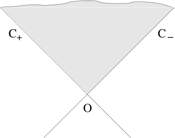
Figure 2: The light cone

In the rest of this paper we will use the “light cone” method for describing the Poisson brackets. Let us briefly explain this. Pick a point $O$ on the worldsheet with the coordinates $(\tau_{0}^{+},\tau_{0}^{-})$ and consider the light cone with the origin at this point, see Fig. 2. The light cone consists of two lines, $C^{+}$ with $\tau^{-}=\tau^{-}_{0}$ and $C^{-}$ with $\tau^{+}=\tau^{+}_{0}$. The solution inside the shaded region is determined by the data $(\varphi,\psi,\lambda)$ on $C^{+}_{\tau^{+}\geq 0}$ and $C^{-}_{\tau^{-}\geq 0}$. Therefore we can describe the Poisson bracket by saying what is the Poisson bracket of the fields on the light cone. The standard Poisson bracket for $\varphi$ would be

$$\{\varphi(\tau_{1}^{+},\tau_{0}^{-}),\varphi(\tau_{2}^{+},\tau_{0}^{-})\}_{usual}={1\over 2}\varepsilon(\tau_{1}^{+}-\tau_{2}^{+})$$

$$\{\varphi(\tau_{0}^{+},\tau_{1}^{-}),\varphi(\tau_{0}^{+},\tau_{2}^{-})\}_{usual}={1\over 2}\varepsilon(\tau_{1}^{-}-\tau_{2}^{-})$$

where $\varepsilon(\tau_{1}-\tau_{2})$ is $1$ if $\tau_{1}>\tau_{2}$ and $-1$ if $\tau_{1}<\tau_{2}$. But this is not the Poisson bracket corresponding to the symplectic form (21). We will now describe on the light cone the Poisson structure corresponding to the symplectic form (21) with the constraint $r_{+}=r_{-}=1$.

3 Poisson structure.

Let ${\cal M}_{\widetilde{O(3)}}$ denote the space of solutions of (13)—(20) and ${\cal M}_{\widetilde{CS}}$ denote the space of solutions with $r_{+}=r_{-}=1$. (The index CS stands for “classical string”, and the tilde reminds us that we are considering the T-dual model.) Let us denote ${\cal M}_{SG}$ the space of $\varphi$ solving the sine-Gordon equation. We have seen that ${\cal M}_{\widetilde{CS}}$ is an affine bundle over ${\cal M}_{SG}$. For a point $x\in{\cal M}_{\widetilde{CS}}$ let us denote ${\cal F}_{x}$ the fiber going through this point. In other words, if $x=(\varphi,\lambda,\psi)$ then ${\cal F}_{x}$ consists of all the solutions of the form $(\varphi,\lambda+\Delta\lambda,\psi+\Delta\psi)$ where $\Delta\lambda$ and $\Delta\psi$ satisfy (27). Let $T_{x}{\cal F}_{x}\subset T_{x}{\cal M}_{\widetilde{CS}}$ be the tangent space to ${\cal F}_{x}$ at the point $x$. Let us denote $\widehat{\cal L}_{x}\subset T_{x}{\cal M}_{\widetilde{CS}}$ the subspace of the tangent space to ${\cal M}_{\widetilde{CS}}$ at the point $x$ consisting of the vectors orthogonal with respect to $\omega$ to $T_{x}{\cal F}_{x}$. In other words, $\widehat{\cal L}_{x}$ is the space of all vectors $\xi\in T_{x}{\cal M}_{\widetilde{CS}}$ such that for any $\eta\in T_{x}{\cal F}_{x}$ we have $\omega(\xi,\eta)=0$. Schematically: $\widehat{\cal L}_{x}=(T_{x}{\cal F}_{x})^{\perp}$. Let us denote ${\cal L}_{\varphi}=\widehat{\cal L}_{x}/T{\cal F}_{x}$. We will view ${\cal L}_{\varphi}$ as a subspace in the tangent space to ${\cal M}_{SG}$. We have a distribution of planes ${\cal L}_{\varphi}\subset T_{\varphi}{\cal M}_{SG}$. We will now show that this distribution is integrable and defines a foliation of ${\cal M}_{SG}$ of the codimension three.

Let us first introduce some notations. When we write a differential operator in the space of functions of $\tau^{+}$ we understand that each operator $\partial_{+}={\partial\over\partial\tau^{+}}$ acts on everything to the right of it. For example:

$$\partial_{+}f_{1}f_{2}=f_{1}\partial_{+}f_{2}+f_{2}\partial_{+}f_{1}$$

But if a part of the expression is inside the $\langle\rangle$ brackets, then any $\partial_{+}$ inside the brackets acts only on everything to the right of it inside the brackets, but not to the right of the $\rangle$ bracket. For example:

$$\langle\partial_{+}f_{1}f_{2}\rangle f_{3}=f_{2}f_{3}\partial_{+}f_{1}+f_{1}f_{3}\partial_{+}f_{2}$$

$$\partial_{+}f_{1}\langle\partial_{+}f_{2}\rangle f_{3}=f_{3}\langle\partial_{+}f_{2}\rangle\partial_{+}f_{1}+f_{1}f_{3}\partial_{+}^{2}f_{2}+f_{1}\langle\partial_{+}f_{2}\rangle\partial_{+}f_{3}$$

Let us denote by $L_{+}$ the operator:

$$L_{+}=\partial_{+}q_{+}^{-1}(1+\partial_{+}^{2})+4q_{+}\partial_{+}$$ (31)

and by $L_{+}^{T}$ its conjugate:

$$L_{+}^{T}=-(1+\partial_{+}^{2})q_{+}^{-1}\partial_{+}-4\partial_{+}q_{+}$$ (32)

Eq. (29) can be written as:

$$L_{+}\psi=2$$

For a function $f(\tau^{+})$ consider the tangent vector $V_{f}$ to the phase space ${\cal M}_{SG}$ given by the equation:

$$V_{f}q_{+}=-L_{+}^{T}f$$ (33)

Notice that ${\cal L}_{\varphi}$ is generated by vectors of the form $V_{f}$ for all the possible functions $f$. Let us compute the commutator $[V_{g},V_{f}]$:

$$[V_{f},V_{g}].q_{+}=$$

$$=-(1+\partial_{+}^{2})q_{+}^{-1}\left(q_{+}^{-1}\partial_{+}f\partial_{+}^{2}q_{+}^{-1}\partial_{+}g+4\langle\partial_{+}q_{+}q_{+}^{-1}\rangle g\partial_{+}f-(f\leftrightarrow g)\right)+$$

$$+\left(4\partial_{+}\langle(1+\partial_{+}^{2})q_{+}^{-1}\partial_{+}g+4\partial_{+}q_{+}g\rangle f-(f\leftrightarrow g)\right)=V_{[f,g]}.q_{+}$$ (34)

where

$$[f,g]=-\langle q_{+}^{-1}\partial_{+}f\rangle\stackrel{{\scriptstyle\leftrightarrow}}{{\partial_{+}}}\langle q_{+}^{-1}\partial_{+}g\rangle+4f\stackrel{{\scriptstyle\leftrightarrow}}{{\partial_{+}}}g$$ (35)

This verifies the Frobenius condition and shows that the distribution ${\cal L}_{\varphi}$ is integrable. This means that the sine-Gordon phase space is foliated by submanifolds of codimension three such that the tangent space to the submanifold at the point $\varphi$ is precisely ${\cal L}_{\varphi}$. We will denote these submanifolds by the same letter ${\cal L}_{\varphi}$. We will say more about the geometrical meaning of ${\cal L}_{\varphi}$ in the next section.

If $\xi\in{\cal L}_{\varphi}$ and $\zeta$ is tangent to the fiber (that is, $\zeta$ changes only $\psi$ and does not affect $\varphi$) then $\omega(\xi,\zeta)=0$. Therefore $\omega$ correctly defines a 2-form on each ${\cal L}_{\varphi}$. We will denote this 2-form by the same letter $\omega$. Let us evaluate $\omega(V_{f},V_{g})$. We have:

$$\omega=\delta\alpha,\;\;\;\alpha=\int d\tau^{+}\psi\delta q_{+}$$

$$\omega(V_{f},V_{g})=V_{f}.\alpha(V_{g})-V_{g}.\alpha(V_{f})-\alpha([V_{f},V_{g}])$$

Notice that

$$\alpha(V_{g})=-\int d\tau^{+}\langle L_{+}^{T}g\rangle\psi=-\int d\tau^{+}gL\psi=-2\int d\tau^{+}g$$

Therefore $V_{f}.\alpha(V_{g})=0$ and we have:

$$\omega(V_{f},V_{g})=-\alpha([V_{f},V_{g}])=2\int d\tau^{+}[f,g]=4\int d\tau^{+}f(\partial_{+}q_{+}^{-1}\partial_{+}q_{+}^{-1}\partial_{+}+4\partial_{+})g$$

This means that on ${\cal L}_{\varphi}$:

$$\omega=4\int d\tau^{+}\delta q_{+}L_{+}^{-1}(\partial_{+}q_{+}^{-1}\partial_{+}q_{+}^{-1}\partial_{+}+4\partial_{+})(L_{+}^{T})^{-1}\delta q_{+}$$ (36)

Of course this form is well-defined only if both $\delta q_{+}$ are tangent to ${\cal L}_{\varphi}$. The corresponding Poisson structure $\theta=\omega^{-1}$ is a bivector tangent to ${\cal L}_{\varphi}$:

$$\theta=L_{+}^{T}(\partial_{+}q_{+}^{-1}\partial_{+}q_{+}^{-1}\partial_{+}+4\partial_{+})^{-1}L_{+}$$ (37)

This formula means that the Poisson bracket between $q_{+}$ on the light cone $C^{+}$ is:

$$\{q_{+}(\tau_{1}^{+}),q_{+}(\tau_{2}^{+})\}=\theta\delta(\tau_{1}^{+}-\tau_{2}^{+})$$ (38)

where the operator $\theta$ acting on the delta-function on the right hand side is given by the formula (37) with $q_{+}=q_{+}(\tau^{+}_{1})$ and $\partial_{+}={\partial\over\partial\tau^{+}_{1}}$. Yet another way to say it is that, given the functional $F$ on the phase space of the sine-Gordon model, the Hamiltonian vector field generated by $F$ using the Poisson structure $\theta$ is:

$$\dot{q}(\tau^{+})=\theta{\delta F\over\delta q_{+}}(\tau^{+})$$ (39)

where $\delta F$ is the variational derivative of $F$. It is useful to compare (39) to the Hamiltonian vector field generated by $F$ using the standard Poisson structure $\theta_{0}=\partial_{+}$. The standard Poisson structure would be $\{q_{+}(\tau_{1}^{+}),q_{+}(\tau_{2}^{+})\}=\delta^{\prime}(\tau_{1}^{+}-\tau_{2}^{+})$, and the standard Hamiltonian vector field of $F$ would be $\dot{q}=\partial_{+}{\delta F\over\delta q_{+}}$, for example $F=\int d\tau^{+}\cos 2\varphi$ would generate $\dot{q}=2\sin 2\varphi=-4\partial_{-}q_{+}$.

Notice that Eq. (37) can be written as:

$$\theta=-(\theta_{1}+\theta_{0})\theta_{1}^{-1}(\theta_{1}+\theta_{0})$$ (40)

Here $\theta_{0}=\partial_{+}$ is the standard Poisson structure of sine-Gordon and $\theta_{1}$ is the second Poisson structure:

$$\theta_{1}=\partial_{+}^{3}+4\partial_{+}q_{+}\partial_{+}^{-1}q_{+}\partial_{+}$$ (41)

Two Poisson brackets are called compatible if their sum is again a Poisson bracket (satisfies the Jacobi identity). Eq. (40) shows that $\theta$ is compatible with the standard Poisson structure of the sine-Gordon. Indeed, the compatibility of two brackets $\theta_{a}$ and $\theta_{b}$ is a bilinear condition, which we can denote $[\![,]\!]$:

$$[\![\theta_{a},\theta_{b}]\!]=0$$

The bilinear operation $[\![,]\!]$ is called Schouten bracket. It follows from our construction that $\theta=(\theta_{0}+\theta_{1})\theta_{1}^{-1}(\theta_{0}+\theta_{1})$ is a Poisson bracket: $[\![\theta,\theta]\!]=0$ (because it corresponds to the closed 2-form $\omega$). We have to prove that $[\![\theta,\theta_{0}]\!]=0$. We have $[\![\theta_{0},\theta_{1}]\!]=0$ because $\theta_{0}$ and $\theta_{1}$ are compatible Poisson structures of the sine-Gordon model (we know it from [22]). Given that $\theta=\theta_{1}+2\theta_{0}+\theta_{0}\theta_{1}^{-1}\theta_{0}$ we have to prove that $[\![\theta_{0},\theta_{0}\theta_{1}^{-1}\theta_{0}]\!]=0$. This is true because $\theta_{0}^{-1}+\varepsilon\theta_{1}^{-1}$ is a closed 2-form for an arbitrary $\varepsilon$; therefore $(\theta_{0}^{-1}+\varepsilon\theta_{1}^{-1})^{-1}$ is a Poisson structure for an arbitrary $\varepsilon$; at the first order in $\varepsilon$ this means that $[\![\theta_{0},\theta_{0}\theta_{1}^{-1}\theta_{0}]\!]=0$.

Let us rewrite $\theta$ in the following way:

$$\theta=-\theta_{1}-2\theta_{0}-(\partial_{+}+4q_{+}\partial_{+}^{-1}q_{+})^{-1}$$ (42)

where

$$\theta_{0}=\partial_{+}$$

$$\theta_{1}=\partial_{+}^{3}+4\partial_{+}q_{+}\partial_{+}^{-1}q_{+}\partial_{+}$$ (43)

This means that although $\theta$ is nonlocal, the nonlocality is rather weak. There are two nonlocal pieces. One is coming from $\partial_{+}^{-1}$ in $\theta_{1}$. This can be represented by one integration:

$$\partial_{+}^{-1}f(\tau)={1\over 2}\int d\tau_{1}\varepsilon(\tau-\tau_{1})f(\tau_{1})$$ (44)

The other nonlocality comes from

$$(\partial_{+}+4q_{+}\partial_{+}^{-1}q_{+})^{-1}={1\over 2}\left({1\over\partial_{+}+2iq_{+}}+{1\over\partial_{+}-2iq_{+}}\right)$$ (45)

The kernel of this operator also requires just one integration:

$$f(\tau)\mapsto{1\over 2}\int d\tau_{1}\varepsilon(\tau-\tau_{1})\cos[2\varphi(\tau)-2\varphi(\tau_{1})]f(\tau_{1})$$ (46)

Given a functional $F$ on the phase space, we can consider the corresponding Hamiltonian vector field

$$\dot{q}=\theta\delta F$$

The nonlocality of the Poisson bracket leads to some ambiguities in the definition of $\dot{q}$. One ambiguity comes from the nonlocality in (45), and the other one from the $\partial^{-1}$ in $\theta_{1}$. Therefore $\dot{q}$ is defined up to $C_{1}\partial_{+}q+C_{2}\partial_{-}q$ where $C_{1}$ and $C_{2}$ are constants. This ambiguity reflects the fact that reparametrizations of the worldsheet are gauge symmetries of the string sigma-model. There is also a third ambiguity $\dot{q}=C_{3}\cos 2\varphi$, but we think that this vector field should probably be discarded because of its behaviour at $\tau^{+}=\pm\infty$. Also notice that the vector fields $\dot{q}=\partial_{+}q$ and $\dot{q}=\partial_{-}q$ are strictly speaking not tangent to ${\cal L}_{q}$. Formally $\partial_{+}q=L_{+}^{T}1$ and $\partial_{-}q=L_{+}^{T}\cos(2\varphi)$, but $1$ and $\cos 2\varphi$ are not going to zero at infinity. If this is a problem, it should be resolved by imposing the appropriate periodicity conditions.

In some sense, the nonlocality of $\theta$ could reflect the fact that the classical string is perhaps more sensitive to the boundary conditions than the standard sine-Gordon model.

4 Classical string and its dual.

In this section we will consider the usual classical string with the action $\int d\tau^{+}d\tau^{-}(\partial_{+}{\bf n},\partial_{-}{\bf n})$. With the periodic boundary conditions the string worldsheet has a topology of the cylinder, and the string phase space is a principal $O(3)$ bundle over the subspace of the sine-Gordon phase space [20]. We will here choose different boundary conditions. Let us consider the classical strings interpolating between the two fixed lightlike geodesics. This means that in the conformal coordinates ${\bf n}(\tau,\sigma)|_{\sigma=-\infty}$ and ${\bf n}(\tau,\sigma)|_{\sigma=+\infty}$ are two different equators of the sphere. On the field theory side this corresponds to an infinite spin chain interpolating between two different BMN vacua [23]. We will call these boundary conditions the “BMN boundary conditions”. These boundary conditions break the $O(3)$ invariance. Therefore we now have a map into the sine-Gordon phase space on an infinite line, which is an injective map rather than a projection. We want to describe the symplectic form on the image of this map which corresponds to the symplectic form of the classical string. We will do it by comparing the classical string to its dual.

Let us consider the extended classical theory which has fields $\lambda,\psi$ and $\phi_{\pm},A_{\pm}$ and besides that also the field $\bf n$ with the values in $S^{2}$, and some choice of the basis in the tangent space to $S^{2}$. The relation between $\bf n$ and $\phi_{\pm}$ is

$$\phi_{\pm}^{i}=({\bf e}^{i},\partial_{\pm}{\bf n})$$ (47)

where ${\bf e}^{i}$ is the basis in the tangent space. The equations of motion for the fields are (5)—(10). Consider the one-form $\hat{\alpha}$ on this extended phase space, given by the following integral of the local expression over the spacial contour:

$$\hat{\alpha}=\oint\left[(\lambda,\delta\phi_{-})d\tau^{-}+(\lambda,\delta\phi_{+})d\tau^{+}+\right.$$

$$+\psi\delta A_{-}d\tau^{-}+\psi\delta A_{+}d\tau^{+}-$$

$$\left.-(\delta{\bf n},\partial_{-}{\bf n})d\tau^{-}+(\delta{\bf n},\partial_{+}{\bf n})d\tau^{+}\right]$$ (48)

This integral does not depend on the choice of the contour. We will denote $\widehat{\cal M}$ the phase space of this extended model, ${\cal M}_{\widetilde{CS}}$ the phase space considered in Section 3 and ${\cal M}_{CS}$ the usual phase space of the classical string parametrized by ${\bf n}(\tau,\sigma)$. Notice that the difference of the symplectic forms $\omega_{CS}$ and $\omega_{\widetilde{CS}}$ on the extended phase space is the differential of $\hat{\alpha}$:

$$\omega_{\widetilde{CS}}-\omega_{CS}=\delta\hat{\alpha}$$ (49)

If we considerd periodic boundary conditions on ${\bf n}$ then there would be some ambiguity in restoring ${\bf n}$ from the sine-Gordon solution, because of the global $O(3)$ symmetry. But with the BMN boundary conditions the $O(3)$ is broken and there is no ambiguity.

We will now see that the 1-form $\hat{\alpha}$ actually vanishes. We can describe $\hat{\alpha}$ in the following way. Let us compare the actions of the $O(3)$ model and its dual:

$$S_{O(3)} = \int(\partial_{+}{\bf n},\partial_{-}{\bf n})$$ (50)

$$S_{\widetilde{O(3)}} = \int\left[(\phi_{+},(1-\psi I)\phi_{-})+\right.$$ (51)

$$\left.+(\lambda,(D_{+}\phi_{-}-D_{-}\phi_{+}))+\psi(\partial_{+}A_{-}-\partial_{-}A_{+})\right]$$

Notice that the difference of these two actions is zero on the equations of motion:

$$(S_{\widetilde{O(3)}}-S_{O(3)})_{on-shell}=0$$ (52)

Let us consider some finite region $D$ on the worldsheet and change the classical solution inside this region to the other classical solution. Under the infinitesimal variation of the classical solution inside $D$ the variation of $S_{\widetilde{O(3)}}-S_{O(3)}$ is equal to the integral (48) over the contour $\partial D$. But $S_{\widetilde{O(3)}}-S_{O(3)}$ is identically zero on the classical solutions. This shows that the integral (48) over the closed contour is zero, and therefore $\hat{\alpha}$ does not depend on the choice of the contour.

Let us now impose the Virasoro constraints $r_{\pm}=1$ and fix the gauge $\phi_{\pm}=e^{\pm i\varphi}$. Then the 1-form $\hat{\alpha}$ becomes:

$$\hat{\alpha}=\oint \left[\psi\stackrel{{\scriptstyle\leftrightarrow}}{{\partial}}_{+}\delta\varphi\;d\tau^{+}-\psi\stackrel{{\scriptstyle\leftrightarrow}}{{\partial}}_{-}\delta\varphi\;d\tau^{-}+\right.$$ (53)

$$\left.+(\delta{\bf n},\partial_{+}{\bf n})d\tau^{+}-(\delta{\bf n},\partial_{-}{\bf n})d\tau^{-}\right]$$

We have seen that the phase space ${\cal M}_{\widetilde{CS}}$ (the dual of the classical string) is an affine bundle over the sine-Gordon phase space, and we denoted ${\cal L}_{\varphi}$ the foliation by the integral manifolds of the distribution of the symplectic complements of the tangent space to the fiber. It turns out that for the fixed BMN boundary conditions, the image of the classical string phase space ${\cal M}_{CS}$ in the sine-Gordon phase space is precisely one of those integral manifolds ${\cal L}_{\varphi}$. To understand this, we have to explain how to lift the tangent space to ${\cal L}_{\varphi}$ to the tangent space of ${\cal M}_{CS}$. The tangent space to ${\cal L}_{\varphi}$ consists of the variations of the form:

$$\delta q_{+}=-L^{T}_{+}f_{+},\;\;\;\delta q_{-}=-L^{T}_{-}f_{-}\;\;\;$$ (54)

$$\mbox{where }\;q_{\pm}=\partial_{\pm}\varphi={1\over 2}\partial_{\pm}\arccos(\partial_{+}{\bf n},\partial_{-}{\bf n})\;$$

We assume that both $f_{+}$ and $f_{-}$ are rapidly decreasing at the spacial infinity. To find the lift $\delta{\bf n}$ it is useful to consider the 1-form $\hat{\alpha}$. Let us restrict ourselves to the $C^{+}$ characteristic:

$$\hat{\alpha}=\int_{C^{+}}\left[2\psi\delta q_{+}d\tau^{+}+(\delta{\bf n},\partial_{+}{\bf n})d\tau^{+}\right]$$ (55)

If $\delta\varphi$ satisfies (54) with $f_{+}$ sufficiently rapidly decreasing at $\tau^{+}=\pm\infty$ then:

$$\int_{C^{+}}2\psi\delta q_{+}d\tau^{+}=-4\int_{C^{+}}f_{+}d\tau^{+}$$ (56)

For each tangent vector to ${\cal L}_{\varphi}$ we have to find the corresponding lift $\delta{\bf n}$ such that $\delta\varphi=\delta\left({1\over 2}\arccos(\partial_{+}{\bf n},\partial_{-}{\bf n})\right)$ satisfies (54). The lift should be in the kernel of $\hat{\alpha}$, because otherwise the phase space of the classical string would have a 1-form given by the integral of a local expression. Eqs. (55) and (56) suggests that we define $\delta{\bf n}$ by the following equation:

$$(\delta{\bf n},\partial_{\pm}{\bf n})=4f_{\pm}$$ (57)

This is consistent with Eq. (54). Indeed, Eq. (57) implies that the variation of the field $\bf n$ is given by the following formula:

$$\delta{\bf n}={4\over\sin^{2}2\varphi}\left[(f_{+}-f_{-}\cos 2\varphi)\partial_{+}{\bf n}+(f_{-}-f_{+}\cos 2\varphi)\partial_{-}{\bf n}\right]$$ (58)

The equations of motion for $f_{+}$ and $f_{-}$ follow from the constraints $(\partial_{+}{\bf n},\partial_{+}{\bf n})=1$ and $(\partial_{-}{\bf n},\partial_{-}{\bf n})=1$:

$$f_{-}=-{\sin 2\varphi\over 2q_{+}}\partial_{+}f_{+}+f_{+}\cos 2\varphi$$ (59)

$$f_{+}=-{\sin 2\varphi\over 2q_{-}}\partial_{-}f_{-}+f_{-}\cos 2\varphi$$ (60)

These two equations imply:

$$\partial_{+}f_{-}=-{1\over 2}\sin 2\varphi\partial_{+}q_{+}^{-1}\partial_{+}f_{+}-2q_{+}\sin 2\varphi f_{+}$$ (61)

and

$$\partial_{+}\left({\partial_{-}f_{+}\over\sin(2\varphi)}\right)=-{1\over 2}q_{+}^{-1}\partial_{+}f_{+}$$ (62)

This means that:

$$\delta q_{+}=-2\partial_{+}\left({\partial_{+}f_{-}+\partial_{-}f_{+}\over\sin 2\varphi}\right)=-L^{T}_{+}f_{+}$$ (63)

This shows the consistency of (54) with (57),  (58).

We see that the one-form $\hat{\alpha}$ vanishes on the lift of ${\cal L}_{\varphi}$. Therefore Eq. (49) implies that the symplectic form on ${\cal L}_{\varphi}$ following from the classical string is given by the same formula (36) as the symplectic form following from the dual of the classical string. In this sense, we can say that as classical field theories, the theory (50) and its dual (51) are equivalent modulo some zero modes which are not visible in the sine-Gordon description.

The general fact of the canonicity of the nonabelian duality was discussed in [8, 24, 25, 26].

5 Summary

We considered the nonabelian dual of the classical string on ${\bf R}\times S^{2}$. We have shown that there is a projection map from the phase space of this model to the phase space of the sine-Gordon model. The space of functionals on the phase space of the classical string has a subspace consisting of the functionals of the sine-Gordon field $\varphi$. This subspace is closed under the Poisson bracket of the classical string, which corresponds to the nonlocal Poisson bracket (42) of the sine-Gordon. This nonlocal Poisson bracket is compatible with the canonical Poisson bracket of the sine-Gordon which comes from the sine-Gordon action. (In a sense that their sum is also a Poisson bracket.)

This suggests that the quantization (after imposing the Virasoro constraints) of the string sigma-model on ${\bf R}\times S^{2}$ could be closely related to the quantization of the sine-Gordon model with the nonlocal Poisson structure (42). But notice that the correspondence works only after imposing the Virasoro constraints. From the point of view of the string theory, it would be interesting to find a good integrable description of the string worldsheet CFT without imposing the Virasoro constraints.

References

• [1] K. Pohlmeyer, “Integrable hamiltonian systems and interactions through quadratic constraints,” Commun. Math. Phys. 46 (1976) 207–221.
• [2] A. Gorsky, A. Marshakov, A. Orlov, and V. Rubtsov, “On third Poisson structure of KdV equation,” Theor. Math. Phys. 103 (1995) 701–705, hep-th/9503018.
• [3] A. Y. Maltsev and S. P. Novikov, “On the local systems Hamiltonian in the weakly non-local Poisson brackets,” Phys. D 156 (2001), no. 1-2, 53–80.
• [4] K. Zarembo, “Semiclassical Bethe ansatz and AdS/CFT,” Comptes Rendus Physique 5 (2004) 1081–1090, hep-th/0411191.
• [5] B.E. Fridling, A. Jevicki, “Dual representations and ultraviolet divergences in nonlinear sigma models”, Phys.Lett. B134 (1984) 70.
• [6] E.S. Fradkin, A.A. Tseytlin, “Quantum equivalence of dual field theories”, Annals Phys. 162 (1985) 31.
• [7] X. de la Ossa, F. Quevedo, “Duality symmetries from nonabelian isometries in string theory”, Nucl.Phys. B403 (1993) 377-394, hep-th/9210021.
• [8] T. Curtright, C.K. Zachos, “Canonical nonabelian dual transformations in supersymmetric field theories” Phys.Rev. D52 (1995) 573-576, hep-th/9502126.
• [9] A. Doliwa and P. M. Santini, “An Elementary geometric characterization of the integrable motions of a curve,” Phys. Lett. A185 (1994) 373–384.
• [10] J. Langer, “Recursion in curve geometry,” New York J. Math. 5 (1999) 25–51 (electronic).
• [11] J. Langer and R. Perline, “Poisson geometry of the filament equation,” J. Nonlinear Sci. 1 (1991), no. 1, 71–93.
• [12] G. Marí Beffa, J. A. Sanders, and J. P. Wang, “Integrable systems in three-dimensional Riemannian geometry,” J. Nonlinear Sci. 12 (2002), no. 2, 143–167.
• [13] J. A. Sanders and J. P. Wang, “Integrable systems in $n$-dimensional Riemannian geometry,” Mosc. Math. J. 3 (2003), no. 4, 1369–1393.
• [14] G. Marí Beffa, “Poisson brackets associated to invariant evolutions of Riemannian curves,” Pacific J. Math. 215 (2004), no. 2, 357–380.
• [15] G. Marí Beffa, “Poisson brackets associated to the conformal geometry of curves,” Trans. Amer. Math. Soc. 357 (2005), no. 7, 2799–2827 (electronic).
• [16] G. Marí Beffa, “Poisson geometry of differential invariants of curves in some nonsemisimple homogeneous spaces,” Proc. Amer. Math. Soc. 134 (2006), no. 3, 779–791 (electronic).
• [17] A. Mikhailov, ”Bihamiltonian structure of the classical superstring in $AdS_{5}\times S^{5}$”, hep-th/0609108.
• [18] I. Bena, J. Polchinski, and R. Roiban, “Hidden symmetries of the AdS(5) x S**5 superstring,” Phys. Rev. D69 (2004) 046002, hep-th/0305116.
• [19] N. Beisert, V. A. Kazakov, K. Sakai, and K. Zarembo, “The algebraic curve of classical superstrings on AdS(5) x S**5,” hep-th/0502226.
• [20] A. Neveu, N. Papanicolaou, “Integrability of the classical scalar and symmetric scalar-pseudoscalar contact Fermi interactions in two-dimensions,” Commun.Math.Phys. 58 (1978) 31.
• [21] N. Papanicolaou, “Gravitational duality and Bäcklund transformations”, J.Math.Phys. 20 (1979) 2069.
• [22] A. S. Fokas, P. J. Olver, and P. Rosenau, “A plethora of integrable bi-Hamiltonian equations,” Progr. Nonlinear Differential Equations Appl. 26 (1997) 93–101.
• [23] D. Berenstein, J. Maldacena and H. Nastase, ”Strings in Flat Space and PP-Waves from ${\cal N}=4$ Super Yang-Mills”, JHEP 0204 (2002) 013, hep-th/0202021.
• [24] C. Klimčík, P. Ševera “Dual nonabelian duality and the Drinfeld double”, Phys.Lett. B351 (1995) 455-462, hep-th/9502122.
• [25] Y. Lozano, “Nonabelian duality and canonical transformations”, Phys.Lett. B355 (1995) 165-170, hep-th/9503045.
• [26] K. Sfetsos, “Canonical equivalence of nonisometric sigma models and Poisson-Lie T duality”, Nucl.Phys. B517 (1998) 549-566, hep-th/9710163.