Scalar Casimir effect between Dirichlet spheres or a plate and a sphere

Abstract

We present a simple formalism for the evaluation of the Casimir energy for two spheres and a sphere and a plane, in case of a scalar fluctuating field, valid at any separations. We compare the exact results with various approximation schemes and establish when such schemes become useful. The formalism can be easily extended to any number of spheres and/or planes in three or arbitrary dimensions, with a variety of boundary conditions or nonoverlapping potentials/nonideal reflectors.

I Introduction

In 1948 the Dutch physicist Hendrik Casimir predicted the existence of a very peculiar effect, the attraction between two metallic uncharged parallel plates in vacuum casimir . The existence of such an attraction has been confirmed experimentally with high accuracy only recently lamoureaux ; bordag . However, nearly all modern experiments (the noted exceptions are the two-cylinder work of Ref. ederth and the two-plate experiment of Ref. bressi ) study the attraction between a metallic sphere and a metallic plate which are much simpler to align than two plates, but much harder to calculate. In fact, with the exception of the proximity-force approximation prox1 ; prox2 , which is only applicable for vanishing separation, there does not exist a theoretical prediction for the Casimir energy of the sphere-plate system as function of the distance.

The origin of this attractive force can be traced back to the modification in the spectrum of zero point fluctuations of the electromagnetic field when the separated mirrors are brought into close distance. Similar phenomena are expected to exist for various other (typically bosonic) fields others ; kardar and the corresponding forces are referred to as Casimir or fluctuation-induced interactions. A related interaction arises when the space is filled with fermions, which is particularly relevant to the physics of neutron stars nm ; mh ; earlier ; bw01 ; bhmwy03 ; bmw05 and quark gluon plasma qgp .

Since the Casimir effect between a sphere and a plate is the experimentally interesting but theoretically difficult case, because of the electromagnetic nature of the fluctuating fields, the corresponding Casimir effect for a real scalar field between two spheres or one sphere and a plate came into the focus of theoretical research sspra ; ssprl ; gies1 ; gies2 ; emig ; jaffe ; scardI ; scardII ; scardIII . Therefore we will here focus on the exact and semiclassical calculation of this scalar Casimir effect between spheres or spheres and plates in three spatial dimensions, where we assume Dirichlet boundary conditions on the spheres and plates. This scenario can be trivially extended to the case of Neumann or other boundary conditions, to two-dimensional systems of disks and/or lines and to analogous systems in arbitrary dimensions. We will show that the Casimir force calculation for the two-sphere case incorporates the sphere-plate geometry as special case. Note that, with the exception of the numerical results of Refs. gies1 ; gies2 (see also emig ), which do not yet extend to large separations, no exact result exists in the literature for the Casimir effect for a real scalar field under Dirichlet boundary conditions, neither between a sphere and a plate nor between two spheres. For small separations between the sphere and the plate, the above-mentioned proximity-force approximation prox1 ; prox2 can be applied. Its justification at small separations has been provided by many authors using various theoretical techniques. For instance, in Refs. sspra ; ssprl semiclassical methods in the framework of the Gutzwiller trace formula gutbook have been used, in Ref. balian3 the proximity-force approximation for the electromagnetic case has been derived from the multiple scattering expansion of Ref. balian12 , in Refs. gies1 ; gies2 the world-line approach in the framework of the Feynman path integral has been applied, and in Refs. jaffe ; scardI ; scardII ; scardIII a ray-dynamical approach in terms of optical paths (i.e. closed but not necessarily periodic orbits) has been employed.

Here, we will present an evaluation of the scalar Casimir problem that is based on quantum mechanics, without any semiclassical approximation made beforehand. It utilizes the Krein formula krein ; uhlenbeck as a bridge between the spectral density on the one hand and the problem of scattering of a point particle between spheres in three dimensions (or disks in two dimensions) on the other hand. It has to be emphasized that in this case the Casimir calculation is not plagued by the removal of diverging ultra-violet contributions. This is related to the fact that the Krein formula is exact, and that the determinants of the S-matrix and the corresponding inverse multi-scattering matrix for a system of $N$ nonoverlapping spheres (or disks), which both are manifestly known, are finite wreport ; wh98 ; hwg97 . In this work we do not consider the material dependent stress of, e.g., the deformation of a single spherical shell which was discussed in Ref. graham .

The paper is organized as follows: first, we formulate the problem in terms of the density of states of the scalar field and relate it to the S-matrix of the system using the Krein formula. In Section III we focus on the particular realization of the Casimir effect for the sphere-sphere and the sphere-plate system. Section IV is devoted to investigations of the large-distance limit between spheres where the asymptotic expressions are derived and discussed. Section V discusses the link between the presented approach and the semiclassical methods based on the Gutzwiller trace formula. Finally, the numerical results, approximate expressions and conclusions are presented in Sections VI and VII. For the sake of completeness, the derivation of proximity-force approximation for the sphere-sphere and sphere-plate system is given in Appendix A and a comparison to the two-dimensional two-disk and disk-line systems can be found in Appendix B.

II The modified Krein formula

Our main goal is to reach a qualitative understanding of the scalar Casimir energy at zero temperature in the case of more complicated geometries than the original two-plate system. For that purpose let us consider the fluctuating real scalar field between $N$ nonoverlapping, nontouching, impenetrable spheres of radii $a_{i}$ ($i=1,\dots,N$). It is assumed that that the scalar field is noninteracting and is subject to Dirichlet boundary conditions on the surfaces of the spheres. The spheres are positioned at fixed relative distances $r_{ij}=L_{ij}+a_{i}+a_{j}>a_{i}+a_{j}$ between their centers; $L_{ij}$ is then the shortest relative distance between their surfaces, and $\vec{r}_{ij}$ is the center-to-center distance vector, which includes also the information about the spatial orientation. In order to calculate the Casimir energy we shall represent the smoothed bosonic density of states of the scalar field as a function of the energy $\varepsilon$ (smoothing is over an energy interval $\Delta\varepsilon$ larger than the level spacing in the big volume $V$ of the entire system):

$$g\bigl{(}\varepsilon,\{a_{i}\},\{\vec{r}_{ij}\}\bigr{)}= g_{0}(\varepsilon)+\sum_{i=1}^{N}g_{W}(\varepsilon,a_{i})$$ (1)

$$\text{}+g_{\rm C}\left(\varepsilon,\{a_{i}\},\{\vec{r}_{ij}\}\right),$$

where $g\bigl{(}\varepsilon,\{a_{i}\},\{\vec{r}_{ij}\}\bigr{)}$ is the total density of states of the scalar field, $g_{0}(\varepsilon)$ is the density of states in the absence of all scatterers, and $g_{W}(\varepsilon,a_{i})$ is the correction to the density of states arising from the presence of one sphere (sphere $i$). Clearly $\sum_{i=1}^{N}g_{W}(\varepsilon,a_{i})$ is the correction due to the $N$ spheres infinitely far apart from each other that sums up the excluded volume effects, surface contributions and Friedel oscillations caused by each of the obstacles separately. Finally $g_{\rm C}\bigl{(}\varepsilon,\{a_{i}\},\{\vec{r}_{ij}\})\bigr{)}$ is the remaining part, which is of central interest to us here. It vanishes in the limit of infinitely separated scatterers and is the only term in the density of states which reflects the relative geometry-dependence of the problem. Only this term contributes to the Casimir energy.

Strictly speaking, only the smoothed level densities $g_{W}(\varepsilon)$ and $g_{\rm C}(\varepsilon)$ are finite, whereas the level densities $g(\varepsilon)$ and $g_{0}(\varepsilon)$ are infinite, as they are proportional to the volume $V$ of the entire space. This redundant divergence can be handled easily by considering the smoothed quantities first in a very big box, the volume of which is subsequently taken to infinitywreport .

Now we will use the Krein formula krein ; uhlenbeck which provides a link between the ($N$-body) scattering matrix $S_{N}(\varepsilon)$ of a point-particle scattering off $N$ spheres and the change in the density of states due to the presence of $N$ scatterers, namely

$$\delta g\bigl{(}\varepsilon,\{a_{i}\},\{\vec{r}_{ij}\}\bigr{)}=g\bigl{(}\varepsilon,\{a_{i}\},\{\vec{r}_{ij}\}\bigr{)}-g_{0}(\varepsilon)$$

$$=\frac{1}{2\pi{\rm i}}\;\frac{d\ }{d\varepsilon}\ln\det S_{N}\bigl{(}\varepsilon,\{a_{i}\},\{\vec{r}_{ij}\}\bigr{)}\,.$$ (2)

Note that $\ln\det S_{N}\bigl{(}\varepsilon,\{a_{i}\},\{\vec{r}_{ij}\}\bigr{)}/2{\rm i}$ is nothing else than the total phase shift of the scattering problem. The geometry-dependent part of the density of states can now be extracted from the genuine multi-scattering determinant. In this way the calculation is mapped onto a quantum mechanical billiard problem that classically corresponds to the hyperbolic (or even chaotic) point-particle scattering off $N$ spheres hwg97 (or $N$ disks in two dimensions  Eck_org ; gasp ; Cvi_Eck_89 ; pinball ; aw_chaos ; aw_nucl ; vwr94 ; rvw96 ).

As shown in Refs. wreport ; wh98 ; hwg97 , the determinant of the $N$-scatterer S-matrix, $S_{N}\bigl{(}\varepsilon,\{a_{i}\},\{\vec{r}_{ij}\}\bigr{)}$, factorizes into the product of the determinants of the single-scatterer S-matrices and the ratio of the determinants of the inverse multi-scattering matrix wreport ; wh98 ; hwg97 of Korringa–Kohn–Rostoker (KKR) type kkr ; Lloyd ; Lloyd_smith ; berry81 $M(k)=M(k,\{a_{i}\},\{\vec{r}_{ij}\})$ in the complex wave number ($k=|\vec{k}|$) plane:

$$\det S_{N}\bigl{(}\varepsilon,\{a_{i}\},\{\vec{r}_{ij}\}\bigr{)}=\left\{\prod_{i=1}^{N}\det S_{1}(\varepsilon,a_{i})\right\}\frac{\det M(k^{*})^{\dagger}}{\det M(k)}.$$ (3)

The formula (3) holds in the case when the scattering modes are free massless fields as well as in the case of free nonrelativistic fields with a mass $m$. Both cases imply different energy dispersion relations, $\varepsilon=\hbar\omega=\hbar ck$ in the massless case or $\varepsilon=\hbar^{2}k^{2}/(2m)$ in the nonrelativistic scenario, respectively.

Although the involved matrices are infinite-dimensional, all determinants are well-defined, as long as the number of spheres is finite and the spheres do neither overlap nor touch. This follows from the trace-class property rs4 ; bs_adv of the matrices $S_{N}-\openone$, $S_{i}-{\openone}$ and $M-{\openone}$ which was shown in Refs. wreport ; wh98 ; hwg97 . 

Inserting the exact expression (3) into the original Krein formula (2), using the decomposition (1) and identifying the “Weyl-type” density of states with the phase shift of the corresponding single scatterer

$$g_{W}(\varepsilon,a_{i})=\frac{1}{2\pi{\rm i}}\;\frac{{\rm d}\ }{{\rm d}\varepsilon}\ln\det S_{1}(\varepsilon,a_{i})\,,$$ (4)

one finds a new Krein-type exact formula bw01 which directly links the geometry-dependent part of the density of states with the inverse multi-scattering matrix

$$g_{\rm C}\bigl{(}\varepsilon,\{a_{i}\},\{\vec{r}_{ij}\}\bigr{)}=\frac{{\rm d}\ }{{\rm d}\varepsilon}\frac{-1}{\pi}{\rm Im}\ln\det M\bigl{(}k(\varepsilon),\{a_{i}\},\{\vec{r}_{ij}\}\bigr{)}\\$$

or

$${\cal N}_{\rm C}\bigl{(}\varepsilon,\{a_{i}\},\{\vec{r}_{ij}\}\bigr{)}=-\frac{1}{\pi}{\rm Im}\ln\det M\bigl{(}k(\varepsilon),\{a_{i}\},\{\vec{r}_{ij}\}\bigr{)}$$ (5)

for the integrated geometry-dependent part of the density of states

$${\cal N}_{\rm C}\bigl{(}\varepsilon,\{a_{i}\},\{\vec{r}_{ij}\}\bigr{)}=\int_{0}^{\varepsilon}{\rm d}\varepsilon^{\prime}g_{\rm C}\bigl{(}\varepsilon^{\prime},\{a_{i}\},\{\vec{r}_{ij}\}\bigr{)}\,.$$ (6)

The exact formula (5) is the central expression of this paper. The Casimir energy itself follows via the integral

$${\cal E}_{\rm C} = \int_{0}^{\infty}{\rm d}\varepsilon\,{\textstyle\frac{1}{2}}\varepsilon\,g_{\rm C}(\varepsilon)=-{\textstyle\frac{1}{2}}\int_{0}^{\infty}{\rm d}\varepsilon\,{\cal N}_{\rm C}(\varepsilon)$$ (7)

$$= \frac{1}{2\pi}\int_{0}^{\infty}{\rm d}\varepsilon\,{\rm Im}\,\ln\det M\!\left(k(\varepsilon)\right)$$

$$= \frac{1}{4\pi{\rm i}}\Biggl{[}\int_{0}^{\infty(1+{\rm i}0_{+})}{\rm d}\varepsilon\,\ln\det M\!\left(k(\varepsilon)\right)$$

$$\qquad\text{}-\int_{0}^{\infty(1-{\rm i}0_{+})}{\rm d}\varepsilon\,\ln\det M\!\left(k^{\ast}(\varepsilon)\right)^{\dagger}\Biggr{]}\,.$$

In the massless case $\varepsilon=\hbar ck$, this expression can be Wick-rotated (i.e., $k\to{\rm i}\,k_{4}$ for the first term and $k\to-{\rm i}\,k_{4}$ for the second term of the last relation) to give 

$${\cal E}_{\rm C} = \frac{\hbar c}{2\pi}\int_{0}^{\infty}{\rm d}k_{4}\,\ln\det M({\rm i}k_{4})\,,$$ (8)

since $\det M(k)=\det M((-k)^{\ast})^{\dagger}$ and therefore $\det M({\rm i}k_{4})=\det M({\rm i}k_{4})^{\dagger}$ if $k_{4}$ real. 

Using the explicit formulas for the KKR–type matrix from Ref. wreport ; wh98 ; hwg97 , one can compute numerically ${\cal E}_{\rm C}$ for various arrangements of hard spherical (or circular in 2D) scatterers. For a point-particle scattering off $N$ nonoverlapping nontouching spheres (under Dirichlet boundary conditions)

$$M^{jj^{\prime}}_{lm,l^{\prime}m^{\prime}}=\delta^{jj^{\prime}}\delta_{ll^{\prime}}\delta_{mm^{\prime}}+(1-\delta^{jj^{\prime}})\,\sqrt{4\pi}\,{\rm i}^{2m+l^{\prime}-l}$$

$$\text{}\times\sqrt{(2l\!+\!1)(2l^{\prime}\!+\!1)}\,\left({\textstyle\frac{a_{j}}{a_{j^{\prime}}}}\right)^{2}\frac{{\rm j}_{l}(ka_{j})}{{\rm h}^{(1)}_{l^{\prime}}(ka_{j^{\prime}})}$$

$$\text{}\times\sum_{l^{\prime\prime}=0}^{\infty}\sum_{m^{\prime\prime}=-l^{\prime}}^{l^{\prime}}{\rm D}^{l^{\prime}}_{m^{\prime}\!,m^{\prime\prime}}(j,j^{\prime})\,{\rm h}^{(1)}_{l^{\prime\prime}}(kr_{jj^{\prime}})\,{{\rm Y}_{l^{\prime\prime}}^{m\!-\!m^{\prime\prime}}\!\bigl{(}\hat{r}^{(j)}_{jj^{\prime}}\bigr{)}}$$

$$\text{}\times\sqrt{2l^{\prime\prime}\!+\!1}\,{\rm i}^{l^{\prime\prime}}\left(\begin{matrix}l^{\prime\prime}&l^{\prime}&l\cr 0&\!0\!&0\end{matrix}\right)\left(\begin{matrix}l^{\prime\prime}&l^{\prime}&l\cr m\!-\!m^{\prime\prime}&\!m^{\prime\prime}\!&-m\end{matrix}\right)$$ (9)

is the inverse multi-scattering matrix hwg97 . Here $j,j^{\prime}=1,2,\dots,N$ are the labels of the $N$ spheres, $l,l^{\prime},l^{\prime\prime}=0,1,2,\dots$ are the angular momentum quantum numbers, and $m,m^{\prime},m^{\prime\prime}$ the pertinent magnetic quantum numbers. ${\rm D}^{l^{\prime}}_{m^{\prime}\!,m^{\prime\prime}}(j,j^{\prime})$ is a Wigner rotation matrix which transforms the local coordinate system from sphere $j^{\prime}$ to the one of sphere $j$, ${\rm j}_{l}(kr)$ and ${\rm h}^{(1)}_{l}(kr)$ are the spherical Bessel and Hankel functions of first kind respectively, ${\rm Y}_{l^{\prime\prime}}^{m\!-\!m^{\prime\prime}}\!\bigl{(}\hat{r}^{(j)}_{jj^{\prime}}\bigr{)}$ is a spherical harmonic (where $\hat{r}^{(j)}_{jj^{\prime}}$ is the unit vector, measured in the local frame of sphere $j$, pointing from sphere $j$ to sphere $j^{\prime}$), and the 3j-symbols landolt result from the angular momentum coupling.

By definition, the inverse multi-scattering matrix incorporates the pruning rule that two successive scatterings have to take place at different scatterers (see the $(1-\delta^{jj^{\prime}})$ term in Eq. (9)). This alternating pattern between a single-scatterer T-matrix and the successive propagation to a new scatterer wreport ; Lloyd ; Lloyd_smith distinguishes the KKR-type method from the multiple scattering expansion of Refs. balian12 ; balian3 .

III The two-sphere and the sphere-plate problem

In the case of two spheres the system possesses a continuous symmetry, i.e. $C_{\infty\,v}$ in crystallography group theory notation hamermesh , associated with rotations with respect to the axis joining the centers of the spheres (and an additional reflection symmetry with respect to any plane containing this symmetry axis). As a consequence the KKR-matrix is separable with respect to the magnetic quantum number $m$ (in fact, it depends on its modulus $|m|$ only) hwg97 . In the global domain, it is given as

$$\left(\begin{matrix}{M}^{11}&{M}^{12}\cr{M}^{21}&{M}^{22}\end{matrix}\right)_{lm,l^{\prime}m^{\prime}}\!\!\!\!\!=\delta_{mm^{\prime}}\left(\begin{matrix}\delta_{ll^{\prime}}&A_{ll^{\prime}}^{12\,(m)}\cr A_{ll^{\prime}}^{21\,(m)}&\delta_{ll^{\prime}}\end{matrix}\right)$$ (10)

with

$$A_{ll^{\prime}}^{jj^{\prime}\,(m)}=(-1)^{l^{\prime}}\,{\rm i}^{l^{\prime}-l}\frac{{a_{j}^{2}\,{\rm j}_{l}(ka_{j})}}{{a_{j^{\prime}}^{2}{\rm h}^{(1)}_{l^{\prime}}(ka_{j^{\prime}})}}\sqrt{(2l\!+\!1)(2l^{\prime}\!+\!1)}$$

$$\text{}\times\sum_{l^{\prime\prime}}{\rm i}^{l^{\prime\prime}}(2l^{\prime\prime}\!+\!1)\left(\begin{matrix}l^{\prime\prime}&l&l^{\prime}\cr 0&\!0\!&0\end{matrix}\right)\left(\begin{matrix}l^{\prime\prime}&l&l^{\prime}\cr 0&\!m\!&-m\end{matrix}\right){\rm h}^{(1)}_{l^{\prime\prime}}(kr).$$

(11)

If the spheres have moreover the same radius $a_{1}=a_{2}\equiv a$, there exist also a two-fold reflection symmetry with respect to the vertical symmetry plane. This additional symmetry makes the total symmetry of the system to be $D_{\infty\,h}$ in the crystallography group notation hamermesh  , which is a simply product of the $C_{\infty\,v}$ group and the inversion (and rotation by $\pi$) with respect to the point of intersection between the symmetry axis and vertical symmetry plane.

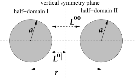
Figure 1: Two identical spheres of radius $a$ at a center-to-center separation $r$. The vertical symmetry plane, the two half-domains and the surface-surface separation $L^{{\rm oo}}$ in the global domain and $L^{{\rm o|}}$ in one of the half-domains are shown.

Therefore the global domain of the two-sphere system can be split into two half-domains, separated by this plane, see Fig. 1, and all the (scattering) wave functions can decomposed into symmetric and antisymmetric ones with respect to the vertical symmetry plane. The symmetric wave functions are subject to Neumann boundary conditions and the antisymmetric are subject to Dirichlet boundary conditions on this symmetry plane. Thus there exist two KKR matrices in the the half-domain hwg97 , one corresponding to the Neumann case (N) and the other, with the additional minus sign, to the Dirichlet case (D):

$$\left.M^{{\rm oo}\,(m)}_{ll^{\prime}}\right|_{\rm N} = \delta_{ll^{\prime}}+A_{ll^{\prime}}^{(m)}\,,$$ (12)

$$\left.M^{{\rm oo}\,(m)}_{ll^{\prime}}\right|_{\rm D} = \delta_{ll^{\prime}}-A_{ll^{\prime}}^{(m)}\,,$$ (13)

where $A_{ll^{\prime}}^{(m)}\equiv\left.A_{ll^{\prime}}^{12\,(m)}\right|_{a_{1}=a_{2}\equiv a}=\left.A_{ll^{\prime}}^{21\,(m)}\right|_{a_{1}=a_{2}\equiv a}$. Furthermore the KKR determinant $\det M^{{\rm oo}}(k,a,r)$ $\equiv$ $\det M^{{\rm o}_{1}{\rm o}_{2}}(k,a_{1}\!=\!a,a_{2}\!=\!a,r)$ of the full domain factorizes into the product of the determinants of these Neumann and Dirichlet KKR matrices

$$\det M^{{\rm oo}}(k,a,r)=\prod_{m=-\infty}^{\infty}\det M^{{\rm oo}\,(m)}(k,a,r)$$

$$=\prod_{m=-\infty}^{\infty}\det\left.M^{{\rm oo}\,(m)}(k,a,r)\right|_{\rm N}\det\left.M^{{\rm oo}\,(m)}(k,a,r)\right|_{\rm D}$$

$$\equiv\det\left.M^{{\rm oo}}(k,a,r)\right|_{\rm N}\det\left.M^{{\rm oo}}(k,a,r)\right|_{\rm D}\,\,.$$ (14)

Thus the two-sphere system contains the Dirichlet sphere-plate system as special case, namely in the symmetric limit $a_{1}=a_{2}=a$, the sphere-plate system is equal the Dirichlet case in the half-domain, and the pertinent multi-scattering determinant $\det M^{{\rm o|}}$ of the sphere-plate system is just given as

$$\det M^{{\rm o|}}\Bigl{(}k,a,L^{\rm o|}\Bigr{)}=\left.\det M^{{\rm oo}}\Bigl{(}k,a,r\!=\!2(L^{\rm o|}\!+\!a)\Bigr{)}\right|_{\rm D}\,.$$ (15)

Note that the shortest surface-to-surface distance in the symmetric two-sphere case is given by $L^{\rm oo}=r-2a$, whereas the shortest surface-to-surface distance in the sphere-plate case is $L^{\rm o|}={\textstyle\frac{1}{2}}r-a$, see Fig. 1.

The exact expressions for the Casimir energy of the two-sphere Dirichlet problem, the symmetric two-sphere Dirichlet problem and the sphere-plate Dirichlet problem are given by the following integrals, respectively:

$${\cal E}_{\rm C}^{{\rm o}_{1}{\rm o}_{2}}(a_{1},a_{2},L)$$

$$=\frac{\hbar c}{2\pi}\int_{0}^{\infty}\!\!\!{\rm d}k_{4}\ln\det M^{{\rm o}_{1}{\rm o}_{2}}({\rm i}k_{4},a_{1},a_{2},r\!=\!L\!+\!a_{1}\!+\!a_{2})\,,$$

$${\cal E}_{\rm C}^{{\rm oo}}(a,L)=\frac{\hbar c}{2\pi}\int_{0}^{\infty}\!\!\!{\rm d}k_{4}\ln\det M^{\rm oo}({\rm i}k_{4},a,r\!=\!L\!+\!2a)\,,$$

$${\cal E}_{\rm C}^{{\rm o|}}(a,L)$$

$$=\frac{\hbar c}{2\pi}\int_{0}^{\infty}\!\!{\rm d}k_{4}\ln\det\left.M^{\rm oo}\bigl{(}{\rm i}k_{4},a,r\!=\!2(L\!+\!a)\bigr{)}\right|_{\rm D}.$$

(16)

In practice, these expressions have to be numerically integrated up to an upper value $k_{4}^{\rm max}$ which should be chosen large enough, such that the numerical value of the integral is stable for some specified range of decimal places. For the sphere-plate case, $k_{4}^{\rm max}\sim 10/L$ specifies a good choice. In order that the evaluation of the determinant of the matrix $\left.M^{\rm oo}_{ll^{\prime}}\bigl{(}m;k,a,r\!=\!2(L\!+\!a)\bigr{)}\right|_{\rm D}$ is stable, the upper value of $k$ induces a maximal value $l_{\rm max}$ for $l,l^{\prime}$ and $m$ (with $|m|\leq l,l^{\prime}\leq l_{\rm max}$), namely berry81 ; wreport

$$l_{\rm max}\geq\frac{{\rm e}}{2}k_{4}^{\rm max}a\approx 14a/L\,.$$ (17)

For small values of the separation $L$, the maximal angular momentum and therefore the size of the KKR matrices (which scale with $l^{2}\times l$ where the last factor results from the separable $m$ quantum number) becomes rapidly very large and limits the range of applicability of this numerical computation of the exact integral to medium and large values of $L$, say, $L>0.1a$, chiefly because of the handling of the 3j-symbols which scale with $l^{4}$.

IV Large-distance limit

As shown in Ref. bw01 , it is possible to obtain significantly simpler expressions for the (integrated) density of states in the limit of very large separation or very small scatterers. If the wave length $\lambda=2\pi/k$ is much larger than the radii of the scatterers one can show that the KKR–matrix $M(k)$ is given by

$$[M(k)]^{jj^{\prime}}\approx\delta^{jj^{\prime}}-(1-\delta^{jj^{\prime}})f_{j}(k)\frac{\exp({\rm i}kr_{jj^{\prime}})}{r_{jj^{\prime}}}$$ (18)

(see rww96 for the analog in the 2D case), where the indices $j,j^{\prime}=1,\dots,N$ denote the scatterers, $r_{jj^{\prime}}$ is the distance between their centers and $f_{j}(k)$ is the $s$-wave scattering amplitude on the $j$–th scatterer.

In the case of two identical spheres of radius $a$, with their centers located at the distance $r$ apart, one obtains

$$\det M(k) = 1-\frac{a^{2}}{r^{2}}\,\exp\left[{\rm i}k(2r-2a)\right]$$

$$= \left.\det M(k)\right|_{N}\left.\det M(k)\right|_{D}$$

$$= \left\{1+\frac{a}{r}{\rm e}^{{\rm i}k(r-a)}\right\}\left\{1-\frac{a}{r}{\rm e}^{{\rm i}k(r-a)}\right\}.$$ (20)

As usual, the determinant of this two-sphere system in the global domain factorizes into two sub-determinants calculated for one of the half-domains, one subject to Neumann boundary conditions and the other (with the minus sign) subject to Dirichlet boundary conditions.

As mentioned, this expression can be derived from Eqs.  (12-13) in the case of large center-to-center separations of spheres, $kr\gg 1$: we can make use of the asymptotic expression for the spherical Hankel function Abramowitz

$${\rm h}^{(1)}_{l}(kr)\sim\frac{\exp({\rm i}kr)}{{\rm i}^{l+1}kr}\,,$$ (21)

which is actually exact for ${\rm h}^{(1)}_{0}(kr)$, such that the inverse multi-scattering matrix becomes

$$M^{{\rm oo}\,(m)}_{l_{1}l_{2}}(k,a,r)\sim\delta_{l_{1}l_{2}}\pm\frac{{\rm j}_{l_{1}}(ka)}{{\rm h}^{(1)}_{l_{2}}(ka)}\,\frac{\sqrt{(2l_{1}\!+\!1)(2l_{2}\!+\!1)}}{{\rm i}^{l_{1}+l_{2}}}$$

$$\times\frac{\exp({\rm i}kr)}{{\rm i}kr}\sum_{l=0}^{\infty}(2l\!+\!1)\left(\begin{matrix}l_{1}&l_{2}&l\cr m&\!-m\!&0\end{matrix}\right)\left(\begin{matrix}l_{1}&l_{2}&l\cr 0&\!0\!&0\end{matrix}\right).$$ (22)

Using now the orthogonality relation for the $3j$–symbols landolt

$$\sum_{l=0}^{\infty}(2l\!+\!1)\!\left(\begin{matrix}l_{1}&l_{2}&l\cr m_{1}&\!m_{2}\!&m\end{matrix}\right)\!\left(\begin{matrix}l_{1}&l_{2}&l\cr m_{1}^{\prime}&\!m_{2}^{\prime}\!&m\end{matrix}\right)\!\!=\delta_{m_{1}m_{1}^{\prime}}\delta_{m_{2}m_{2}^{\prime}},$$

we get the asymptotic result

$$M^{{\rm oo}\,(m)}_{l_{1}l_{2}}(k,a,r)\sim\delta_{l_{1}l_{2}}\pm\frac{{\rm j}_{l_{1}}(ka)}{{\rm h}^{(1)}_{l_{2}}(ka)}$$

$$\qquad\text{}\times\frac{\sqrt{(2l_{1}+1)(2l_{2}+1)}}{{\rm i}^{l_{1}+l_{2}}}\,\frac{\exp({\rm i}kr)}{{\rm i}kr}\,\delta_{m0}.$$ (23)

Since for $kr\gg 1$ the only nontrivial matrix $M^{{\rm oo}\,(0)}_{l_{1}l_{2}}$ is separable in $l_{1}$ and $l_{2}$, the corresponding determinant is simply given by

$$\det M^{\rm oo}(k,a,r)$$

$$\sim 1\!-\!\frac{\exp(2{\rm i}kr)}{({\rm i}kr)^{2}}\left[\sum_{l=0}^{\infty}(-1)^{l}(2l\!+\!1)\frac{{\rm j}_{l}(ka)}{{\rm h}^{(1)}_{l}(ka)}\right]^{2}$$

$$\equiv 1-\frac{\exp(2{\rm i}kr)}{(kr)^{2}}\,\left[-{\rm i}A(ka)\right]^{2}.$$ (24)

for the identical two-sphere case and by

$$\det M^{\rm o|}(k,a,L)\equiv\det\left.M^{\rm oo}\bigl{(}k,a,r\!=\!2(L\!+\!a)\bigr{)}\right|_{\rm D}$$

$$\sim 1\!-\!\frac{\exp({\rm i}kr)}{{\rm i}kr}\sum_{l=0}^{\infty}(-1)^{l}(2l\!+\!1)\frac{{\rm j}_{l}(ka)}{{\rm h}^{(1)}_{l}(ka)}$$

$$\equiv 1-\frac{\exp({\rm i}kr)}{kr}\,\left(-{\rm i}A(ka)\right)$$ (25)

for the sphere-plate case. Here

$$A(ka)\equiv\sum_{l=0}^{\infty}(-1)^{l}(2l\!+\!1)\frac{{\rm j}_{l}(ka)}{{\rm h}^{(1)}_{l}(ka)}$$ (26)

is the multipole expansion of the scattering amplitude. For $ka\ll 1$, the ratio ${\rm j}_{l}(ka)/{\rm h}^{(1)}_{l}(ka)$ becomes Abramowitz

$$\frac{{\rm j}_{l}(ka)}{{\rm h}^{(1)}_{l}(ka)} = \frac{{\rm i}(ka)^{2l+1}{\rm e}^{-{\rm i}ka}}{1^{2}\times 3^{2}\times\cdots\times(2l-1)^{2}\times(2l+1)}$$ (27)

$$\text{}+{\cal O}\left((ka)^{2l+2+\delta_{l,0}}\right).$$

Thus the dominant effect comes from the $s$-wave scattering only and the $l>0$ terms can be neglected. Consequently, the scattering amplitude becomes

$$-{\rm i}A(ka) = -{\rm i}\frac{{\rm j}_{0}(ka)}{{\rm h}^{(1)}_{0}(ka)}+{\cal O}\left((ka^{3})\right)$$ (28)

$$= ka\exp(-{\rm i}ka)+{\cal O}\left((ka^{3})\right)\,,$$

which implies that (24) becomes (IV) and (25) becomes the Dirichlet part of (20).

If the determinant in the global domain (IV) is inserted into the modified Krein formula (5) we get the following result for the integrated geometry-dependent part of the density of states in the $s$-wave limit of the two-sphere case bw01 (note $r=L^{\rm oo}+2a$):

$${\cal{N}}_{s-{\rm wave}}^{\rm oo}(\varepsilon)=\frac{a^{2}}{\pi(L^{\rm oo}\!+\!2a)^{2}}\sin\left[2k(L^{\rm oo}\!+\!a)\right]+{\cal{O}}\left((ka)^{3}\right).$$ (29)

Analogously one gets the $s$-wave limit for the Dirichlet sphere-plate system by inserting the Dirichlet determinant of the half-domain, namely the second term of Eq.(20), into (5):

$${\cal{N}}_{s-{\rm wave}}^{\rm o|}(\varepsilon)=\frac{a}{2\pi(L^{\rm o|}\!+\!a)}\sin\left[k(2L^{\rm o|}\!+\!a)\right]+{\cal{O}}\left((ka)^{3}\right)$$ (30)

[note $r=2(L^{\rm o|}+a)$].

Now, the Casimir energy for two identical Dirichlet spheres in the large $L=L^{\rm oo}$ limit follows simply by inserting ${\cal N}_{s-{\rm wave}}^{\rm oo}$, Eq. (29), into the integral (7) and performing the Wick-rotation as in (8):

$${\cal{E}}_{s-{\rm wave}}^{\rm oo}(a,L)=-\hbar c\frac{a^{2}}{4\pi(L+a)(L+2a)^{2}}$$

$$=\kappa\frac{\pi a^{2}}{L^{3}}\left(\frac{90}{\pi^{4}}\right)\frac{4}{\left(1+\frac{a}{L}\right)\left(1+\frac{2a}{L}\right)^{2}}\,,$$ (31)

where

$$\kappa=-\frac{\hbar c}{16\pi^{2}}\,\frac{\pi^{4}}{90}=-\frac{\hbar c\pi^{2}}{1440}$$ (32)

is the prefactor of the Casimir energy

$${\cal E}^{||}(L)=-\frac{\hbar c\pi^{2}}{2\times 720}\,\frac{A}{L^{3}}$$ (33)

of the corresponding scalar (Dirichlet) two-plate system where $A$ is the area of the plates. Instead of performing the Wick rotation, one can compute these integrals along the real axis too. In this case one would have to include a convergence factor $\exp(-\eta\varepsilon)$ and take the limit $\eta\rightarrow+0$ at the end of the calculation (in a similar manner to the Feynman prescription for propagators).

Similarly, the Casimir energy for the Dirichlet sphere-plate case in the large $L=L^{\rm o|}$ limit follows by inserting ${\cal N}_{s-{\rm wave}}^{\rm o|}$, Eq. (30), into the integral (7) and performing the Wick-rotation:

$${\cal{E}}_{s-{\rm wave}}^{\rm o|}(a,L)=-\hbar c\frac{a}{4\pi(L+a)(2L+a)}$$

$$=\kappa\frac{\pi a}{L^{2}}\left(\frac{90}{\pi^{4}}\right)\frac{2}{\left(1+\frac{a}{L}\right)\left(1+\frac{a}{2L}\right)}\,.$$ (34)

The large-distance scaling is therefore proportional to $a/L^{2}$, in contrast to the Casimir-Polder energy between a molecule and a conducting plane which scales like $a^{3}/L^{4}$ polder . The difference is associated with the fact that the Casimir-Polder energy results from the induced dipole moment, whereas in the scalar scattering the monopole term gives the dominant contribution. In fact, if one omits the $s$-wave scattering term and starts instead with the the $p$-wave term in the scattering function $A(ka)$, the scalar Casimir energy for the sphere-plate system would show a large-$L$ behaviour

$${\cal{E}}_{p-{\rm wave}}^{\rm o|}(a,L) = \kappa\frac{\pi a^{3}}{L^{4}}\left(\frac{90}{\pi^{4}}\right)\frac{1}{\left(1\!+\!\frac{a}{L}\right)\left(1\!+\!\frac{a}{2L}\right)^{2}}\,$$ (35)

which is compatible with the $a^{3}/L^{4}$ scaling of the Casimir-Polder energy. Thus the correct large-distance behaviour of the scalar Casimir energy has nothing to do with missing diffraction contributions (see Refs. aw_chaos ; aw_nucl ; vwr94 ; rvw96 ) to the semiclassical trace formula as conjectured in Ref. sspra and repeated in Ref. scardI . It is rather based on the replacement of the semiclassical summation, which we will discuss in the next section and which is valid when many partial amplitudes contribute, by the leading term(s) in the multipole expansion rww96 ; bw01 .

In summary, the asymptotic expressions for the Casimir energy are given by

$${\cal{E}}_{\rm C}^{\rm oo}({L\gg a})\ \sim\ 4\times\frac{90}{\pi^{4}}\,\frac{\kappa\pi a^{2}}{L^{3}}\approx 3.6958\frac{\kappa\pi a^{2}}{L^{3}}$$ (36)

in the symmetric two-sphere scalar Dirichlet case and by

$${\cal{E}}_{\rm C}^{\rm o|}({L\gg a})\ \sim\ 2\times\frac{90}{\pi^{4}}\,\frac{\kappa\pi a}{L^{2}}\approx 1.8479\frac{\kappa\pi a}{L^{2}}$$ (37)

in the sphere-plate scalar Dirichlet case.

V The semiclassical approximation

The semiclassical approximation of the scalar two-sphere problem in the framework of the Gutzwiller trace formula gutbook was pioneered in Refs. sspra ; ssprl . Here we will focus on the link between the scattering approach and these semiclassical methods.

The sphere-plate system at surface-to-surface separation $L$ is a special case of the sphere-sphere case for two spheres of radii $a_{1}$ and $a_{2}$ at center-to-center separation $R=L+a_{1}+a_{2}$ in the limit $a_{2}\to\infty$. As shown in Ref. bw01 , the integrated density of states for the two-sphere system follows semiclassically from the Gutzwiller trace formula gutbook

$${\cal N}^{{\rm o}_{1}{\rm o}_{2}}_{\rm sc}(a_{1},a_{2},L,k)$$

$$=\frac{1}{\pi}{\rm Im}\,\sum_{n=1}^{\infty}\frac{\exp(n{\rm i}2kL)}{n}\frac{1}{|\det\left(\left[{\sf M}(a_{1},a_{2},L)\right]^{n}-{\openone}\right)|^{1/2}}$$

$$=\frac{1}{\pi}{\rm Im}\,\sum_{n=1}^{\infty}\frac{1}{n}\frac{\exp(n{\rm i}2kL)}{|\Lambda_{+}(a_{1},a_{2},L)^{n}+\Lambda_{-}(a_{1},a_{2},L)^{n}-2|}$$

$$=\sum_{n=1}^{\infty}\frac{1}{n\pi}\frac{\sin(n2kL)}{|\Lambda_{+}(a_{1},a_{2},L)^{n}+\Lambda_{-}(a_{1},a_{2},L)^{n}-2|},$$ (38)

where the periodic orbit is the bouncing-orbit between the spheres and the summation is over the repeats of this orbit. The matrix ${\sf M}(a_{1},a_{2},L)$ is the monodromy matrix of the sphere-sphere system and $\Lambda_{+}(a_{1},a_{2},L)$ = $1/\Lambda_{-}(a_{1},a_{2},L)$ is the double–degenerate leading eigenvalue of this matrix, i.e.:

$$\Lambda_{\pm}(a_{1},a_{2},L) = 1+2L\left(\frac{1}{a_{1}}\!+\!\frac{1}{a_{2}}\right)+2\frac{L^{2}}{a_{1}a_{2}}$$

$$\pm\sqrt{\left(1\!+\!2L\left(\frac{1}{a_{1}}\!+\!\frac{1}{a_{2}}\right)\!+\!2\frac{L^{2}}{a_{1}a_{2}}\right)^{2}-1}\,,$$

which is identical with Eq. (3.11) of Ref. sspra .

In fact, the semiclassical expression (38) is consistent with the semiclassical limit to the exact expression (5): In Ref.hwg97 it was argued for the two-sphere case and in Ref.wreport it was shown for any $N$-disk case that semiclassically

$$\det M(k)\to\exp\left[-\sum_{p}\sum_{n=1}^{\infty}\frac{1}{n}\,\frac{{\rm e}^{{\rm i}nkl_{p}-{\rm i}\nu_{p}\pi/2}}{\left|\det\left(\left[{\sf M}_{p}\right]^{n}-\openone\right)\right|^{1/2}}\right],$$ (40)

where $l_{p}$, ${\sf M}_{p}$ and $\nu_{p}$ are the total geometrical length, the monodromy matrix and the Maslov index of the $p$-th primitive periodic orbit, respectively. The r.h.s. of (40) is the Gutzwiller-Voros zeta function DasBuch . Note that for our scalar Dirichlet case there exists only one orbit, the bouncing-orbit for the two-sphere (two-disk) system with $l_{p}=2L$, and that the Maslov index is simply $\nu_{p}=4$ because of the two Dirichlet reflections (per repeat). 

If the semiclassical expression (38) is inserted into the Casimir-energy integral (see bw01 )

$${\cal E}_{\rm sc} = {\textstyle\frac{1}{2}}\hbar c\int_{0}^{\infty}{\rm d}k\,k\,\frac{{\rm d}\ }{{\rm d}k}{\cal N}_{\rm sc}(k)$$ (41)

$$= -{\textstyle\frac{1}{2}}\hbar c\int_{0}^{\infty}{\rm d}k\,{\cal N}_{\rm sc}(k)\,,$$

one gets for the scalar sphere-sphere case, after a Wick rotation (as in the transition from (7) to (8)): 

$${\cal E}_{\rm sc}^{{\rm o}_{1}{\rm o}_{2}}(a_{1},a_{2},L)=-{\textstyle\frac{1}{2}}\hbar c\int_{0}^{\infty}{\rm d}k\,{\cal N}^{{\rm o}_{1}{\rm o}_{2}}_{\rm sc}(a_{1},a_{2},L,k)$$

$$=-{\textstyle\frac{1}{2}}\hbar c\sum_{n=1}^{\infty}\frac{1}{n\,\pi}\,\frac{\int_{0}^{\infty}{\rm d}k_{4}\exp(-n2k_{4}L)}{|\Lambda_{+}(a_{1},a_{2},L)^{n}+\Lambda_{-}(a_{1},a_{2},L)^{n}-2|}$$

$$\approx-\frac{\hbar c}{16\pi}\,\frac{a_{1}a_{2}}{L^{2}(a_{1}+a_{2}+L)}\sum_{n=1}^{\infty}\frac{1}{n^{4}}\,$$

$$\ \text{}\times\left[1-\frac{2}{3}\frac{L}{a_{1}\!+\!a_{2}}(n^{2}\!-\!1)-\frac{1}{3}L\frac{a_{1}^{2}+a_{2}^{2}}{a_{1}a_{2}(a_{1}\!+\!a_{2})}(n^{2}\!-\!1)\right]$$

$$\approx-\frac{\hbar c}{16\pi}\,\frac{a_{1}a_{2}}{L^{2}(a_{1}+a_{2}+L)}\left(\frac{\pi^{4}}{90}\right)\Biggl{[}1$$

$$\ \text{}-\frac{2L}{a_{1}\!+\!a_{2}}\left(\frac{5}{\pi^{2}}\!-\!\frac{1}{3}\right)-\frac{L(a_{1}^{2}+a_{2}^{2})}{a_{1}a_{2}(a_{1}\!+\!a_{2})}\left(\frac{5}{\pi^{2}}\!-\!\frac{1}{3}\right)\Biggr{]}.$$

(42)

Here we applied the following identity

$$\Lambda_{+}(a_{1},a_{2},L)^{n}+\Lambda_{-}(a_{1},a_{2},L)^{n}-2$$

$$=4n^{2}\Biggl{[}\frac{L}{a_{1}}+\frac{L}{a_{2}}+\frac{L^{2}}{a_{1}a_{2}}+\frac{2}{3}\frac{L^{2}}{a_{1}a_{2}}(n^{2}-1)$$

$$\qquad\ \text{}+\frac{1}{3}\left(\frac{L^{2}}{a_{1}^{2}}+\frac{L^{2}}{a_{2}^{2}}\right)(n^{2}-1)+{\cal O}\left(\frac{L^{3}}{a_{i}^{3}}\right)\Biggr{]},$$ (43)

which is exact for the case $n=1$, and used

$$\sum_{n=1}^{\infty}\frac{1}{n^{4}}=\frac{\pi^{4}}{90}\quad\text{and}\quad\sum_{n=1}^{\infty}\frac{1}{n^{2}}=\frac{\pi^{2}}{6}\,.$$

Particularly, in the case of two identical spheres of radius $a$ at center-to-center separation $R=L+2a$ one gets a simplified expression

$${\cal E}_{\rm sc}^{{\rm oo}}(a,L)\equiv{\cal E}_{\rm sc}^{{\rm o}_{1}{\rm o}_{2}}(a,a,L)=$$

$$-\frac{\hbar c}{16\pi}\frac{a^{2}}{L^{2}(2a\!+\!L)}\left(\frac{\pi^{4}}{90}\right)\!\left[1\!-\!2\left(\frac{5}{\pi^{2}}\!-\!\frac{1}{3}\right)\frac{L}{a}\!+\!{\cal O}\!\left(\frac{L^{2}}{a^{2}}\right)\right]$$

$$=\kappa\frac{\pi a^{2}}{L^{2}(2a\!+\!L)}\left[1-2\left(\frac{5}{\pi^{2}}\!-\!\frac{1}{3}\right)\frac{L}{a}+{\cal O}\left(\frac{L^{2}}{a^{2}}\right)\right]\,.$$ (44)

It is remarkable that the leading term is exactly equal to the plate-based prediction of the proximity-force approximation for two identical spheres sspra (more details in Appendix A):

$${\cal E}_{\rm plate\,PFA}^{{\rm oo}} = \kappa\frac{\pi a^{2}}{L^{2}(2a+L)}\;.$$ (45)

As mentioned above, the sphere-plate system is a special case of the two-sphere system:

$${\cal E}_{\rm sc}^{{\rm o}|}(a,L)\equiv\lim_{a_{2}\to\infty}{\cal E}_{\rm sc}^{{\rm o}_{1}{\rm o}_{2}}(a,a_{2},L)=$$

$$-\frac{\hbar c}{16\pi}\,\frac{a}{L^{2}}\left(\frac{\pi^{4}}{90}\right)\left[1-\left(\frac{5}{\pi^{2}}-\frac{1}{3}\right)\,\frac{L}{a}+{\cal O}\left([L/a]^{2}\right)\right]$$

$$=\kappa\frac{\pi a}{L^{2}}\left[1-\left(\frac{5}{\pi^{2}}-\frac{1}{3}\right)\,\frac{L}{a}+{\cal O}\left([L/a]^{2}\right)\right]\,.$$ (46)

This expression agrees with Eq. (11) of Ref. schroeder . Note that

$$-{\cal E}_{\rm sc}^{{\rm o}|}(a,L)<-\kappa\frac{\pi a}{L^{2}}\,.$$ (47)

Moreover, the leading $\kappa\pi a/L^{2}$ behaviour of (46) agrees with the leading terms of the plate-based and sphere-based proximity-force approximations for the Dirichlet sphere-plate problem, respectively (see Refs. gies1 ; jaffe ; scardI )

$${\cal E}_{\rm plate\,PFA}^{{\rm o}|} = \kappa\frac{\pi a}{L^{2}}\,\frac{1}{1+L/a}\,,$$ (48)

$${\cal E}_{\rm sphere\,PFA}^{{\rm o}|} = \kappa\frac{\pi a}{L^{2}}\,\Biggl{\{}1-3{\textstyle\frac{L}{a}}-6\left({\textstyle\frac{L}{a}}\right)^{2}$$ (49)

$$\mbox{}\times\Bigl{[}1-\left(1+{\textstyle\frac{L}{a}}\right)\ln(1+a/L)\Bigr{]}\Biggr{\}}.$$

More details about the proximity-force approximation of the Dirichlet sphere-plate system can be found in Appendix A.

The sphere-plate result (46) can also be derived from the Dirichlet part of the identical-two-sphere result using

$${\cal N}_{\rm sc}^{\rm o|} = \left.{\cal N}_{\rm sc}^{\rm oo}\right|_{\rm D}$$ (50)

$$= \frac{1}{\pi}{\rm Im}\sum_{n=1}^{\infty}\frac{1}{n}\frac{\exp\left[{\rm i}n(r-2a)k\right]}{\left|\Lambda_{+}(a,r)^{n}+\Lambda_{-}(a,r)^{n}-2\right|}\,$$

where (compare with Eqs. (38) and (LABEL:Lambda_pm))

$$\Lambda_{\pm}(a,r) \equiv \frac{r}{a}-1\pm\sqrt{\left(\frac{r}{a}-1\right)^{2}-1}$$ (51)

$$= 1+2\frac{L^{\rm o|}}{a}\pm\sqrt{\left(1+2\frac{L^{\rm o|}}{a}\right)^{2}-1}$$

$$= \lim_{a_{2}\to\infty}\Lambda_{\pm}(a_{1}=a,a_{2},L=L^{\rm o|})$$

under $r=2(L^{\rm o|}+a)$. Note that

$$\Lambda_{\pm}(a,r)^{2} = \Lambda_{\pm}(a_{1}=a,a_{2}=a,L=L^{\rm oo})$$ (52)

for $r=L^{\rm oo}+2a$, such that for two identical spheres the integrated density of states is semiclassically

$${\cal N}_{\rm sc}^{\rm oo}=\frac{1}{\pi}{\rm Im}\sum_{n=1}^{\infty}\frac{1}{n}\frac{\exp\left({\rm i}n2(r-2a)k\right)}{\left|\Lambda_{+}(a,r)^{2n}+\Lambda_{-}(a,r)^{2n}-2\right|}\,.$$ (53)

VI Results

The results and approximations, discussed in the previous sections for the Casimir energy ${\cal E}_{\rm C}^{0|}(a,L)$ for the scalar Dirichlet sphere-plate case in units of $\kappa\pi a/L^{2}=-\hbar c\pi^{3}a/(1440L^{2})$ are shown in Fig. 2 as function of the ratio $L/a$.

\psfrag{L/a}{\LARGE$L/a$}\psfrag{-E/hbar c pi**3/1440 L**2}{\LARGE${\cal E}^{\rm o|}_{\rm C}(a,L)\,/\,\frac{-\hbar c\pi^{3}a}{1440L^{2}}$}\includegraphics[width=341.43306pt,angle={-90}]{sphereplate2.eps}

Figure 2: Predictions for the scalar Casimir energy ${\cal E}_{\rm C}^{0|}(a,L)$ of the sphere-plate configuration with Dirichlet boundary conditions are shown in units of $\kappa\pi a/L^{2}$ as function of the ratio $L/a$. The points and curves are explained in the text, see Section VI.

This figure should be compared with Fig. 8 of the world-line approach of Ref. gies1 and with Fig. 4 of the optical approach of Ref.scardI which both only present data for $L/a\leq 4$. The circles (a) represent the numerically calculated exact expression (16) for the sphere-plate system between $L=0.1a$ and $L=512a$ (the line is only there to guide the eye), the curve (b) shows the $s$-wave approximation (34), the line (c) represents the asymptotic limit 1.847 of (37), the curve (d) represents the numerically calculated (Wick-rotated) integral (41) over the semiclassical expression (50) including all repeats, and the line (e) shows the analytical semiclassical formula (46) valid modulo ${\cal O}\bigl{(}(L/a)^{2}\bigr{)}$ corrections. The curve (f) is the result of the plate-based proximity-force approximation (48), and the curve (g) represents the result of the sphere-based proximity-force approximation (49).

Our numerically calculated data (a) agree for $L/a\leq 1$ with the in Ref. gies1 published data of the world-line approach, within the quoted (statistical) error bars which are already sizable at $L/a=1$. We have included these world-line data, which cover the range from $L=a/256$ to $L=4a$, in Fig.2 and marked them by stars (h). Note that their central values are systematically on the low side in comparison to ours. All our data beyond $L=4a$ are predictions. In the meantime, after the first version of this paper was submitted, there appeared in gies2005 new data in the world-line approach with improved systematics which cover the extended range from $L=a/512$ to $L=16a$ and which have smaller, but still sizable error bars for $L\geq a$ (see the crosses (k) in Fig. 2). In the region of overlap, thus now also for the points $L/a=2,4,8,16$, the new world-line data do nicely agree with ours when the quoted statistical error bars are taken into account, although their central values are now systematically higher. It should also be remarked that our smallest point $L=0.1a$ is already affected by a sizable truncation error in the integration. Of course this problem is a matter of numerics and not a matter of principle.

Note that the $s$-wave approximation becomes a reasonable approximation to the exact data from $L\geq 4a$ (it works very nicely for $L>15a$ in agreement with the estimate (17)) and, moreover, that the exact data indeed converge to the predicted asymptotic value $180/\pi^{4}$ of Eq. (37) and do not show any Casimir-Polder $a^{3}/L^{4}$ scaling. It is also interesting that the exact data, at least for the $L$ values for which they could be calculated, are larger than 1 (in units of $\kappa\pi a/L^{2}$), whereas the semiclassical approximation and the proximity-force approximations are strictly less than 1 (in the same units). It should be noted that (at least) the upper error ranges of the old world-line data of Ref. gies1 , the complete new world-line data of Ref. gies2005 (with the exception of the lower error ranges of the points $L/a=1/64,1/128$) and – below $L\sim 0.1a$ – the results of the improved optical approach of Ref. scardI are larger than 1 as well.

The semiclassical calculation, starts out at a value 1 (in units of $\kappa\pi a/L^{2}$) for $L/a\to 0$, which was predicted by the proximity-force approximation(s) prox1 ; prox2 and confirmed in, e.g., Refs. sspra ; ssprl ; gies1 ; jaffe ; scardI . Then, for intermediate values of $L/a$, however, the semiclassical results, even though smaller than 1, are superior to the results of the proximity-force approximation which become ambiguous gies1 ; jaffe ; scardI . For $L\gg a$, the contributions of the repeats of the bouncing-orbit are strongly suppressed and the numerically calculated semiclassical expression converges to the one-bounce result $-\hbar ca/(16\pi L^{2})=(90/\pi^{4})\times\kappa\pi a/L^{2}$ which is smaller by a factor $1/2$ than the exact asymptotic answer (37).

VII Conclusions

We presented here an exact calculation of the scalar Casimir energy for the case of two spheres and a sphere and a plane. It is based on a new Krein-type formula which directly expresses the geometry-dependent part of the density of states by the inverse multi-scattering matrix of the pertinent scattering problem. Thus the corresponding Casimir energy follows from the energy-integral over the multi-scattering phase shift (the logarithm of the multi-scattering determinant). The calculation is therefore not plagued by subtractions of the single-sphere contributions or by a removal of diverging ultra-violet contributions. The asymptotic limit (37), the presented $s$-wave approximation (34) and all data with $L>4a$ are totally new results. Moreover, contrary to claims in the literature, the Casimir-Polder scaling of the scalar Casimir effect is excluded by our numerical and analytical calculations.

The two-sphere and sphere-plane cases are only two examples, and the formalism presented can be easily extended to any number of spheres and planes as well (or disks and lines in two-dimensions). We have exemplified the calculation of the scalar Casimir energy only for the case of Dirichlet boundary conditions. One can replace the Dirichlet with Neumann boundary conditions or with any other conditions easily, or even replace the scatterers with arbitrary nonoverlapping potentials/nonideal reflectors.

Aside from the exact results we have also discussed several approximation schemes, the large separation limit, the semiclassical limit and the proximity-force approximation. The exact results (which are easy to calculate and are definitely simpler to evaluate than in a path integral approach) should be looked upon as test examples for other approximate methods. These results already show that the proximity formula and the semiclassical/orbit approaches are limited to small separations only, typically much smaller than the curvature radii of the two surfaces.

One can make the argument that the dominant momenta of the fluctuating fields contributing to the Casimir energy at a separation $L$ are of the order $k\approx 1/L$ (see Eq. (17)) and thus for large separations only the $s$-wave scattering is important. This is the main reason why the semiclassical approximation (which is valid when many partial amplitudes contribute) fails at large separations.

Just the opposite is true at small separations, where semiclassics is pretty good and so is the proximity formula, when the separations are smaller by one or, respectively, two orders of magnitude than the curvature radii. The same type of analysis can be straightforwardly extended to cylinders, or even objects with less symmetry (in which case the corresponding individual T-matrices appearing in the inverse multi-scattering matrix (see Ref. Lloyd ; Lloyd_smith ; wreport ) become somewhat more complicated, due to the loss of spherical symmetry).

Appendix A Ambiguity in the proximity-force approximation

The proximity-force approximation (PFA) for the Casimir energy ${\cal E}_{\rm C}$ of two arbitrary smooth surfaces (with Dirichlet boundary conditions for the scalar-field case) is given by the surface integral over the Casimir energy per area which belongs to an equivalent parallel-plate system that locally follows the two surfaces prox1 ; prox2 ; gies1 ; jaffe ; scardI , i.e.

$${\cal E}_{\rm PFA}=\iint_{A}{\rm d}\sigma\ \epsilon\left[z(\sigma)\right].$$ (54)

Here $A$ is the area of one of the opposing surfaces which are locally separated by the (surface-dependent) distance $z(\sigma)$ and $\epsilon\left[z(\sigma)\right]$ is the corresponding Casimir energy per area. In general, the plate segment ${\rm d}\sigma$ is tangential to only one of the surfaces and therefore the local distance vector ${\vec{z}}\,(\sigma)$ is perpendicular only to this surface and not to the other one. Thus ${\cal E}_{\rm PFA}$ is not uniquely defined, since the area $A$ can be either one of the two opposing surfaces (or even one ficticious surface somewhere inbetween). Particularly, for the case of a sphere of radius $a$ and a plate at shortest surface-to-surface separation $L$ we get the following expression for the “sphere-based PFA” gies1 ; jaffe ; scardI , where the local distance vector $\vec{z}(\vec{a})$ is perpendicular to the sphere,

$${\cal E}_{\rm sphere\,PFA}^{{\rm o}|} = \kappa\iint_{\rm half-sphere}a^{2}{\rm d}\Omega^{(2)}\,\frac{1}{\left|\vec{z}(\vec{a})\right|^{3}}$$ (55)

$$= \kappa a^{2}{2\pi}\int_{0}^{\pi/2}{\rm d}\theta\,\sin(\theta)\,\frac{\left[\cos(\theta)\right]^{3}}{\left[L+a-a\cos(\theta)\right]^{3}}$$

$$= \kappa\frac{\pi a}{L^{2}}\,\Biggl{\{}1-3{\textstyle\frac{L}{a}}-6\left({\textstyle\frac{L}{a}}\right)^{2}$$

$$\mbox{}\times\Bigl{[}1-\left(1+{\textstyle\frac{L}{a}}\right)\ln(1+a/L)\Bigr{]}\Biggr{\}}\,.$$

The coefficient $\kappa$ is again the prefactor $\kappa=-\frac{\hbar c\pi^{2}}{1440}$ of the Casimir energy ${\cal E}^{||}(L)=-\frac{\hbar c\pi^{2}}{2\times 720}\,\frac{A}{L^{3}}$ of the corresponding scalar (Dirichlet) two-plate system.

On the other hand, the “plate-based PFA” gies1 ; jaffe ; scardI (i.e., the local distance vector ${\vec{z}}\,(\sigma)$ is perpendicular to the plate) follows from

$${\cal E}_{\rm plate\,PFA}^{{\rm o}|} = \kappa\iint_{x^{2}+y^{2}\leq a^{2}}{\rm d}x\,{\rm d}y\,\frac{1}{\left|\vec{z}(x,y)\right|^{3}}$$ (56)

$$= \kappa\int_{0}^{2\pi}{\rm d}\phi\,\int_{0}^{a}{\rm d}\rho\,\rho\,\frac{1}{\left[L+a-\sqrt{a^{2}-\rho^{2}}\right]^{3}}$$

$$= \kappa\frac{\pi a}{L^{2}}\,\frac{1}{1+L/a}\,.$$

Note that

$$-{\cal E}_{\rm sphere\,PFA}^{{\rm o}|}<-{\cal E}_{\rm plate\,PFA}^{{\rm o}|}<-\kappa\frac{\pi a}{L^{2}}\,.$$ (57)

Finally, the PFA for two spheres of a common radius $a$ and shortest surface-to-surface separation $L$ can be derived from the plate-based PFA (56) of the sphere-plate case, with the fictitious plate on the vertical symmetry plane as in Fig. 1, as follows:

$${\cal E}_{\rm plate\,PFA}^{{\rm oo}} = \kappa\iint_{x^{2}+y^{2}\leq a^{2}}{\rm d}x\,{\rm d}y\,\frac{1}{\left|2\,\vec{z}(x,y)\right|^{3}}$$ (58)

$$= \kappa\pi\int_{0}^{2\pi}\!\!{\rm d}\phi\,\int_{0}^{a}\!\!{\rm d}\rho\,\rho\,\frac{1}{8\left[\frac{L}{2}+a-\sqrt{a^{2}-\rho^{2}}\right]^{3}}$$

$$= \kappa\frac{\pi a}{8\left(\frac{L}{2}\right)^{2}}\,\frac{1}{1+L/2a}=\kappa\frac{\pi a^{2}}{L^{2}(2a+L)}\;.$$

Appendix B Comparison with the two-dimensional two-disk and disk-line systems

The two-dimensional analog of the $N$-sphere matrix in three-dimensions (9) is wreport ; wh98

$${\bf M}^{jj^{\prime}}_{mm^{\prime}}=\delta^{jj^{\prime}}\delta_{mm^{\prime}}+(1-\delta^{jj^{\prime}})\frac{a_{j}{\rm J}_{m}(ka_{j})}{a_{j^{\prime}}{\rm H}^{(1)}_{{m^{\prime}}}(ka_{j^{\prime}})}$$

$$\quad\text{}\times(-1)^{m^{\prime}}{\rm e}^{{\rm i}(m\alpha_{j^{\prime}j}-m^{\prime}\alpha_{jj^{\prime}})}{\rm H}^{(1)}_{m-m^{\prime}}(kr_{jj^{\prime}}),$$ (59)

where $j,j^{\prime}=1,2,\dots,N$ are the labels of the $N$ disks. The integers $m,m^{\prime}$ with $-\infty<m,m^{\prime}<\infty$ are the angular momentum quantum numbers in two-dimensions, $a_{j}$ and $r_{jj`}$ are, as usual, the radius of disk $j$ and the distance between the centers of disk $j$ and $j^{\prime}$, respectively. ${\rm J}_{l}(kr)$ and ${\rm H}^{(1)}_{l}(kr)$ are the ordinary Bessel and Hankel functions of first kind, and $\alpha_{jj^{\prime}}$ is the angle of the of the ray from the origin of disk $j$ to the one of disk $j^{\prime}$ as measured in the local coordinate system of disk $j$.

The two-dimensional analog of the two-sphere KKR-type matrix (10) is aw_chaos ; aw_nucl

$$\left(\begin{matrix}{M}^{11}&{M}^{12}\cr{M}^{21}&{M}^{22}\end{matrix}\right)_{m,m^{\prime}}=\left(\begin{matrix}\delta_{mm^{\prime}}&A_{mm^{\prime}}^{12}\cr A_{mm^{\prime}}^{21}&\delta_{mm^{\prime}}\end{matrix}\right)$$ (60)

with

$$A_{mm^{\prime}}^{jj^{\prime}}=(-1)^{m}\,\frac{a_{j}{\rm J}_{m}(ka_{j})}{a_{j^{\prime}}{\rm H}^{(1)}_{m^{\prime}}(ka_{j^{\prime}})}{\rm H}^{(1)}_{m-m^{\prime}}(kr)\,,$$ (61)

where $r=r_{12}=r_{21}$. The general two-disk system is characterized by a $C_{2v}$ symmetry. If the two disks have a common radius $a$, the global domain of this system is separated by the vertical symmetry axis (instead of plane) into two half-domains. The corresponding symmetry group is now $C_{2h}$ and the KKR-matrix splits into two KKR matrices valid for the half-domains, one corresponding to Neumann (N) boundary conditions of the scattering wave functions on the vertical symmetry axis, the other, with the additional minus sign, corresponding to the Dirichlet (D) case:

$$\left.M^{{\rm oo}}_{mm^{\prime}}\right|_{\rm N} = \delta_{mm^{\prime}}+A_{mm^{\prime}}\,,$$ (62)

$$\left.M^{{\rm oo}}_{mm^{\prime}}\right|_{\rm D} = \delta_{mm^{\prime}}-A_{mm^{\prime}}\,,$$ (63)

where $A_{mm^{\prime}}=A^{12}_{mm^{\prime}}|_{a_{1}\!=\!a_{2}\!=\!a}=A^{21}_{mm^{\prime}}|_{a_{1}\!=\!a_{2}\!=\!a}$.

The two-dimensional KKR-matrix in the large-distance limit reads

$$[M(k)]^{jj^{\prime}}\approx\delta^{jj^{\prime}}-(1-\delta^{jj^{\prime}})f_{j}^{{\rm 2D}}(\varepsilon)\frac{\exp({\rm i}kr_{jj^{\prime}})}{\sqrt{r_{jj^{\prime}}}}$$ (64)

instead of (18). Here $f_{j}^{{\rm 2D}}(\varepsilon)$ is the $s$-wave scattering amplitude in two dimensions.

Since the asymptotic expression of the ordinary Hankel function reads Abramowitz

$${\rm H}^{(1)}_{m}(kr) \sim \sqrt{\frac{2}{\pi kr}}\exp\left[{\rm i}\left(kr-m\frac{\pi}{2}-\frac{\pi}{4}\right)\right]$$ (65)

$$\sim (-{\rm i})^{m}{\rm H}^{(1)}_{0}(kr)\,,$$

Eqs. (62-63) become asymptotically

$$M^{{\rm oo}}_{m_{1}m_{2}}(k,a,r) \sim \delta_{m_{1}m_{2}}\pm(-1)^{m_{1}}\frac{{\rm J}_{m_{1}}(ka)}{{\rm H}^{(1)}_{m_{2}}(ka)}\,$$ (66)

$$\qquad\text{}\times{\rm i}^{m_{2}-m_{1}}\,{\rm H}^{(1)}_{0}(kr)$$

instead of (23). This expression is separable in $m_{1}$ and $m_{2}$. Therefore, the corresponding determinant is asymptotically given by

$$\det M^{\rm oo}(k,a,r)$$

$$\sim 1-\left[{\rm H}^{(1)}_{0}(kr)\right]^{2}\left[\sum_{m=-\infty}^{\infty}(-1)^{m}\frac{{\rm J}_{m}(ka)}{{\rm H}^{(1)}_{m}(ka)}\right]^{2}$$

$$\equiv 1-\left[{\rm H}^{(1)}_{0}(kr)\right]^{2}\left[A(ka)\right]^{2}.$$ (67)

for the identical two-disk case and by

$$\det M^{\rm oo}(k,a,r)$$

$$\sim 1-{\rm H}^{(1)}_{0}(kr)\left[\sum_{m=-\infty}^{\infty}(-1)^{m}\frac{{\rm J}_{m}(ka)}{{\rm H}^{(1)}_{m}(ka)}\right]$$

$$\equiv 1-{\rm H}^{(1)}_{0}(kr)\,\left[A(ka)\right]$$ (68)

for the disk-line case. Note that the asymptotic relation (21) is actually exact for ${\rm h}^{(1)}_{0}(kr)$ and therefore holds also for small $k$-values. For the ordinary Hankel function ${\rm H}^{(1)}_{0}(kr)$, however, the corresponding formula (65) is only an asymptotic relation. Since the Casimir energy receives contributions from all $k<10/L$, it severely worsens the $s$-wave result if ${\rm H}^{(1)}_{0}(kr)$ were replaced by its asymptotic form from (65). Here

$$A(ka)\equiv\sum_{m=-\infty}^{\infty}(-1)^{m}\frac{{\rm J}_{m}(ka)}{{\rm H}^{(1)}_{m}(ka)}$$ (69)

is the multipole expansion of the scattering amplitude in two dimensions. For $ka\ll 1$, the dominant effect comes from the $m=0$ ($s$-wave) contribution and the $|m|>0$ terms can be neglected. The scattering amplitude becomes rww96

$$A(ka) = \frac{{\rm J}_{0}(ka)}{{\rm H}^{(1)}_{0}(ka)}+{\cal O}\left((ka)^{2}\right)$$ (70)

$$= \frac{1}{1\!+\!{\rm i}\frac{2}{\pi}\left[\ln\left(\frac{ka}{2}\right)\!+\!\gamma_{E}\right]}+{\cal O}\!\left((ka)^{2}\right),$$

where $\gamma_{E}=0.577\cdots$ is Euler’s constant. For the asymptotic case $kr>ka_{i}\gg 1$, one finds

$$A(ka_{i})\equiv\sum_{m=-\infty}^{\infty}(-1)^{m}\frac{{\rm J}_{m}(ka_{i})}{{\rm H}^{(1)}_{m}(ka_{i})}\approx\frac{\sqrt{{\rm i}\pi ka_{i}}}{2}{\rm e}^{-2{\rm i}ka_{i}}$$

for the scattering amplitude, such that

$$\det M^{{\rm o}_{1}{\rm o}_{2}} \approx 1-\frac{2}{\pi}\frac{{\rm e}^{2{\rm i}kr}}{{\rm i}kr}A(ka_{1})A(ka_{2})$$ (71)

$$\approx 1-\frac{\sqrt{a_{1}a_{2}}}{2r}\,{\rm e}^{{\rm i}2k(r-a_{1}-a_{2})}\,.$$

In fact, the two-dimensional analogs of the semiclassical expression (44) for the identical two-sphere case and (46) for the sphere-plate case are given by

$${\cal E}^{{\rm oo}}_{{\rm sc}} \approx -\frac{\hbar c}{8\pi}\,\frac{a}{L^{3/2}\sqrt{2a+L}}\sum_{n=1}^{\infty}\frac{1}{n^{3}}$$ (72)

$$= -\frac{\hbar c}{16\pi}\zeta(3)\frac{\sqrt{2}}{L}\sqrt{\frac{a}{L(1+L/2a)}}$$

for the two-disk case and

$${\cal E}^{{\rm o|}}_{{\rm sc}} \approx -\frac{\hbar c}{2}\,\sum_{n=1}^{\infty}\frac{1}{\pi n}\frac{1}{2nL}\frac{1}{2n}\sqrt{\frac{a}{L}}$$ (73)

$$= -\frac{\hbar c\zeta(3)}{16\pi}\frac{2}{L}\frac{\sqrt{a}}{\sqrt{L}}=\kappa_{\rm 2D}\,2\frac{\sqrt{a}}{L\sqrt{L}}$$

for the disk-line case, where

$$\kappa_{\rm 2D}\equiv-\frac{\hbar c}{16\pi}\zeta(3)\ \ \mbox{and}\ \ \zeta(3)\equiv\sum_{n=1}^{\infty}\frac{1}{n^{3}}\approx 1.20205.$$ (74)

The corresponding proximity-force approximation reads in the line-based scenario

$${\cal E}_{\rm line\,PFA}^{{\rm o}|} = \kappa_{\rm 2D}\int_{-a}^{a}{\rm d}x\,\frac{1}{\left(L+a-\sqrt{a^{2}-x^{2}}\right)^{2}}$$ (75)

$$= 2a^{2}\kappa_{\rm 2D}\frac{2\arctan\left(\frac{L+2a}{\sqrt{L(L+a)}}\right)+\frac{\sqrt{L(L+2a)}}{a}}{L(L+2a)\sqrt{L(L+2a)}}$$

$$\approx \kappa_{\rm 2D}\frac{\pi}{\sqrt{2}}\frac{\sqrt{a}}{L\sqrt{L}}\approx\kappa_{\rm 2D}\,2.22144\frac{\sqrt{a}}{L\sqrt{L}}\,.$$

The proximity-force approximation for the disk-line system in the disk-based scenario is given by

$${\cal E}_{\rm disk\,PFA}^{{\rm o}|} = \kappa_{\rm 2D}\,a\int_{-\pi/2}^{\pi/2}{\rm d}\phi\frac{\left[\cos\phi\right]^{2}}{\left(L+a-a\cos\phi\right)^{2}}$$

$$\approx \kappa_{\rm 2D}\frac{\pi}{\sqrt{2}}\frac{\sqrt{a}}{L\sqrt{L}}\approx\kappa_{\rm 2D}\,2.22144\frac{\sqrt{a}}{L\sqrt{L}}$$

as well. Note that in the limit $L/a\to 0$ the two-dimensional semiclassical approximation (73) and the proximity-force approximations (75) and (LABEL:E_C_PFAdisk) do approximately agree, but are not identical. Furthermore, the exact result, in the range where it can be calculated, i.e., for $L>0.1a$, does not scale as $\sqrt{a/L}/L$, but rather as $(a/L)^{1/6}/L$. The $s$-wave result is a good approximation to the exact result for $L>10a$, if ${\rm H}^{(1)}_{0}(kr)$ is not replaced by its asymptotic form (65).

References

• (1) H. B. G. Casimir, Proc. Kon. Ned. Akad. Wetensch. 51, 793 (1948).
• (2) S. K. Lamoreaux, Phys. Rev. Lett 78, 5 (1997); 81, 5475(E) (1998); U. Mohideen and A. Roy, Phys. Rev. Lett. 81, 4549 (1998).
• (3) For a review, see M. Bordag, U. Mohideen, and V. M. Mostepanenko, Phys. Reports 353, 1 (2001).
• (4) Th. Ederth, Phys. Rev. A 62, 062104 (2000).
• (5) G. Bressi, G. Carugno, R. Onofrio, and G. Ruoso, Phys. Rev. Lett. 88, 041804 (2002).
• (6) B. V. Derjaguin, Kolloid Z. 69, 155, 1934; B. V. Derjaguin, I. I. Abrikosova, and E. M. Lifshitz, Quart. Rev. 10, 295 (1956); B. V. Derjaguin and I. I. Abrikosova, Zh. Eksp. Teor. Fiz. 30, 993 (1956) [Sov. Phys. JETP 3, 819 (1957)].
• (7) J. Blocki, J. Randrup, W. J. Swiatecki, and C. F. Tsang, Ann. Phys. (N.Y.) 105, 427 (1977); J. Blocki and W. J. Swiatecki, Ann. Phys. (N.Y.) 132, 53 (1981).
• (8) V. M. Mostepanenko and N. N. Trunov, The Casimir Effect and its Applications (Clarendon, Oxford, 1997); M. E. Fisher and P. G. de Gennes, C.R. Acad. Sci. Ser. B 287, 207 (1978); A. Hanke, F. Schlesener, E. Eisenriegler, and S. Dietrich, Phys. Rev. Lett. 81, 1885 (1998); F. Schlesener, A. Hanke, and S. Dietrich, J. Stat. Phys. 110, 981 (2003), and references therein.
• (9) M. Kardar and R. Golestanian, Rev. Mod. Phys. 71, 1233 (1999), and references therein.
• (10) A. Bulgac and P. Magierski, Nucl. Phys.  A683, 695 (2001); A703, 892(E) (2002) [astro-ph/0002377], and references therein.
• (11) P. Magierski and P.-H. Heenen, Phys. Rev. C 65, 045804 (2002) [nucl-th/0112018].
• (12) A. Bulgac et al., in Proceedings of the International Workshop on Collective Excitations in Fermi and Bose Systems, edited by C.A. Bertulani and M.S. Hussein (World Scientific, Singapore, 1999), pp. 44–61 [nucl-th/9811028]; Y. Yu, A. Bulgac and P. Magierski, Phys. Rev. Lett.  84, 412 (2000) [nucl-th/9902011].
• (13) A. Bulgac and A. Wirzba, Phys. Rev. Lett.  87, 120404 (2001) [nucl-th/0102018].
• (14) A. Bulgac, P. H. Heenen, P. Magierski, A. Wirzba, and Y. Yu, AIP Conf. Proc.  704, 483 (2004) [nucl-th/0311023].
• (15) A. Bulgac, P. Magierski, and A. Wirzba, Europhys. Lett. 72, 327 (2005) [cond-mat/0406255].
• (16) G. Neergaard and J. Madsen, Phys. Rev. D 62, 034005 (2000) and earlier references therein.
• (17) M. Schaden and L. Spruch, Phys. Rev. A 58, 935 (1998).
• (18) M. Schaden and L. Spruch, Phys. Rev. Lett. 84, 459 (2000).
• (19) H. Gies, K. Langfeld, and L. Moyaerts, J. High Energy Phys. 06 (2003) 018. [hep-th/0303264].
• (20) L. Moyaerts, K. Langfeld, and H. Gies, hep-th/0311168.
• (21) T. Emig, cond-mat/0311465.
• (22) R. L. Jaffe and A. Scardicchio, Phys. Rev. Lett.  92, 070402 (2004) [quant-ph/0310194].
• (23) A. Scardicchio and R. L. Jaffe, Nucl. Phys. B704, 552 (2005) [quant-ph/0406041].
• (24) A. Scardicchio and R. L. Jaffe, quant-ph/0507042.
• (25) A. Scardicchio, Phys. Rev. D 72, 065004 (2005) [hep-th/0503170].
• (26) M. C. Gutzwiller, Chaos in Classical and Quantum Mechanics (Springer, New York, 1990).
• (27) R. Balian and B. Duplantier, Proceeedings of 15th SIGRAV Conference on General Relativity and Gravitational Physics, Rome, Italy, 2002 (quant-ph/0408124).
• (28) R. Balian and B. Duplantier, Ann. Phys. (N.Y.) 104, 300 (1977); 112 (1978) 165.
• (29) M. G. Krein, Mat. Sb. (N.S.) 33, 597 (1953); Dokl. Akad. Nauk SSSR 144, 268 (1962) [Sov. Math.-Dokl. 3, 707 (1962)]; M. Sh. Birman and M. G. Krein, Dokl. Akad. Nauk SSSR 144, 475 (1962) [Sov. Math.-Dokl. 3, 740 (1962)]; W. Thirring, Quantum Mechanics of Atoms and Molecules (Springer, New York, 1981), Chap. 3.6; M. Sh. Birman and D. R. Yafaev, St. Petersburg Math. J. 4, 833 (1993).
• (30) E. Beth and G. E. Uhlenbeck, Physica 4, 915 (1937); K. Huang, Statistical Mechanics (John Wiley & Sons, New York, 1987), Chap. 10.3; J. Friedel, Nuovo Cim. Ser. 10 Suppl. 7, 287 (1958). These are particular cases of the Krein formula krein .
• (31) A. Wirzba, Phys. Reports 309, 1 (1999)[chao-dyn/9712015].
• (32) A. Wirzba and M. Henseler, J. Phys. A 31, 2155 (1998) [chao-dyn/9702004].
• (33) M. Henseler, A. Wirzba, and T. Guhr, Ann. Phys. (N.Y.) 258, 286 (1997) [chao-dyn/9701018].
• (34) N. Graham, R. L. Jaffe, V. Khemani, M. Quandt, O. Schröder and H. Weigel, Nucl. Phys. B 677, 379 (2004) [hep-th/0309130].
• (35) B. Eckhardt, J. Phys. A 20, 5971 (1987).
• (36) P. Gaspard and S. A. Rice, J. Chem. Phys. 90, 2225 (1989); 90, 2242 (1989); 90, 2255 (1989).
• (37) P. Cvitanović and B. Eckhardt, Phys. Rev. Lett. 63, 823 (1989).
• (38) B. Eckhardt, G. Russberg, P. Cvitanović, P.E. Rosenqvist, and P. Scherer, in Quantum chaos between order and disorder, edited by G. Casati and B. Chirikov, (Cambridge University press, Cambridge, England, 1995), pp. 405–433.
• (39) A. Wirzba, Chaos 2, 77 (1992).
• (40) A. Wirzba, Nucl. Phys. A560, 136 (1993).
• (41) G. Vattay, A. Wirzba, and P. E. Rosenqvist, Phys. Rev. Lett. 73, 2304 (1994) [chao-dyn/9401007].
• (42) P. E. Rosenqvist, G. Vattay, and A. Wirzba, J. Stat. Phys. 83, 243 (1996) [chao-dyn/9602010].
• (43) J. Korringa, Physica (Amsterdam) 13, 392 (1947); W. Kohn and N. Rostoker, Phys. Rev. 94, 1111 (1954); A. Gonis and W. H. Butler, Multiple Scattering in Solids (Springer, New York, 2000).
• (44) P. Lloyd, Proc. Phys. Soc. 90, 207 (1967).
• (45) P. Lloyd and P. V. Smith, Adv. Phys. 21, 69 (1972).
• (46) M. V. Berry, Ann. Phys. (N.Y.) 131, 163 (1981).
• (47) M. Reed and B. Simon, Analysis of Operators, Methods of Modern Mathematical Physics, (Academic, New York, 1978), Vol. IV, Chap. XIII, Sec. 17.
• (48) B. Simon, Adv. Math. 24 (1977) 244.
• (49) Numerical Tables for Angular Correlation Computations in $\alpha$-, $\beta-$, and $\gamma$-Spectroscopy: 3j-,6j-, 9j-Symbols, F- and $\Gamma$-Coefficients, Landolt-Börnstein, (Springer-Verlag, Berlin, 1968), Band 3.
• (50) M. Hamermesh, Group Theory and Its Applications to Physical Problems (Addison-Wesley, Reading, MA, 1962), Chap. 9-1.
• (51) P. Rosenqvist, N. D. Whelan, and A. Wirzba, J. Phys. A 29, 5441 (1996) [chao-dyn/9602017].
• (52) M. Abramowitz and I. A. Stegun, Handbook of Mathematical Functions with Formulas, Graphs and Mathematical Tables (Dover, New York, 1965).
• (53) H. B. G. Casimir and D. Polder, Phys. Rev. 73, 360 (1948).
• (54) P. Cvitanović et al., Chaos: Classical and Quantum (ChaosBook.org, Copenhagen, 2005).
• (55) O. Schröder, A. Scardicchio and R. L. Jaffe, Phys. Rev. A 72, 012105 (2005) [hep-th/0412263].
• (56) H. Gies and K. Klingmüller, hep-th/0511092.