Holographic decays of large-spin mesons

Abstract:

We study the decay process of large-spin mesons in the context of the gauge/string duality, using generic properties of confining backgrounds and systems with flavour branes. In the string picture, meson decay corresponds to the quantum-mechanical process in which a string rotating on the IR “wall” fluctuates, touches a flavour brane and splits into two smaller strings. This process automatically encodes flavour conservation as well as the Zweig rule. We show that the decay width computed in the string picture is in remarkable agreement with the decay width obtained using the phenomenological Lund model.

.9

1 Introduction

Understanding the gauge/string correspondence in the context of realistic, non-supersymmetric, confining gauge theories remains a major open problem. No fully satisfactory geometries dual to confining gauge theories are known so far, and there are general arguments that, in order to fully describe QCD, one will have to go beyond simple supergravity considerations. Nevertheless, it is quite remarkable that many qualitative properties of confining theories do get reproduced correctly from computations in dual supergravity theories. So far, a large body of work in this field has been concerned with a comparison of hadron spectra with the spectra of states on the gravity side. This is a rather kinematical test, and one wonders whether more dynamical properties, such as decay rates, may perhaps also be captured by the correspondence. In recent work by Sakai and Sugimoto [1] decays of low-spin particles (which are captured by the supergravity and DBI modes) have been considered. The decays of high-spin mesons, which correspond to genuine stringy processes, have, however, not been addressed so far. In the present paper, we initiate the study of high-spin meson decays using the dual string theory description.

\psfrag{lm}{\vbox{\hbox{\small large mass}\hbox{\small flavour brane}}}\psfrag{im}{\vbox{\hbox{\small intermediate mass}\hbox{\small flavour brane}}}\psfrag{wl}{\hbox{\small infrared ``wall''}}\includegraphics[width=281.85034pt]{Ustring.eps}

Figure 1: A high-spin meson composed of heavy quarks, represented in the dual string picture as an open string ending on a flavour brane far away from the infrared “wall”. To good approximation, the string consists of two vertical segments, called “region I” and one horizontal segment, called “region II”.

In the context of gauge/string duality, mesons are incorporated by adding one or more flavour branes into confining dual geometries [2]. In this setup, mesons of low-spin are identified with small fluctuations of the flavour brane. This has allowed for a computation of masses and decay rates, both in the approximation in which the flavour brane is treated as a probe [1, 3] and in the case where the backreaction is taken into account [4]. However, the supergravity (i.e. DBI) approximation is not sufficient to deal with mesons with spin larger than one, which from a phenomenological point of view are at least as important. These mesons are described by genuine string excitations, and their precise treatment would require the quantisation of strings in the confining geometries. Given the complexity of the candidate dual geometries, this is a rather formidable task. However, very high-spin mesons can be described in this set up using semi-classical macroscopic spinning string configurations.

The open string configuration which we will consider is depicted in figure 1. This is a U-shaped string, with its endpoints located on the flavour branes, and which is pulled towards the infrared “wall” by the gravitational potential. It also extends along the “wall”, where it is prevented from collapse by its rigid rotation. This string is equivalent to a system two quarks connected by a flux tube, with masses proportional to the distance from the flavour branes to the “wall”. Thus one can have high-spin mesons with light, medium or heavy quarks. The spectrum exhibits deviation from Regge behaviour with appropriate non-linear corrections which depend on the quark masses [5, 6].

In the present paper we study decays of high-spin mesons in detail, both from a qualitative as well as from a quantitative point of view. Semi-classically, the U-shaped string can decay due to an instability of its endpoints or due to breaking of the string itself. The first type of decay channel is associated to radiation processes on the flavour brane, and will be discussed a separate publication. To describe the second family of decay channels, recall that an open string always has to end on a brane, and that therefore the string can break semi-classically if and only if one (or more) of its middle points touch one of the flavour branes. If no flavour brane is present on the infrared “wall”, then classically this condition is never satisfied for the U-shaped string of figure 1, except at those points where the vertical part of the string intersects a flavour brane (splitting at these points, i.e. of the vertical segments of the string, was analysed in [7] and turns out to be highly suppressed). However, semi-classically, there is a finite probability that the string, due to the quantum fluctuations, touches one of the flavour branes, splits and gets reconnected to it, producing two or more outgoing mesons (i.e. “hanging” open strings, see figure 2).

Therefore, in order to compute the decay rate semi-classically, we need to compute the probability of the horizontal part of the string to touch a flavour brane and the probability that the string splits when it is on the brane. Although the calculation of the string fluctuation probability is a hard task, we have found several simplification and approximation methods which make it feasible. The main idea is to focus on the part of the geometry near the “wall”, and then construct the string wave function in this simplified geometry by semi-classical quantisation (for details see section 4). Once this is achieved, the probability for finding the string at a certain distance from the “wall” can be extracted. On the other hand, for a string which is located on the brane, the probability for it to split at any given point can be computed using the flat space results of Dai and Polchinski [8] and Mitchell and Turok [9]. We expect that these semi-classical computations should capture the main features of the full string decay process. That this is indeed the case can be shown explicitly in flat space, by comparing this splitting rate with a full quantum computation.

\psfrag{flavour brane}{flavour brane}\psfrag{IR wall}{infrared ``wall''}\includegraphics*[width=346.89731pt]{basic_idea.eps}

Figure 2: The basic idea behind the description of high-spin mesons in duals of confining gauge theories (left). The open string corresponding to the meson starts on a flavour brane, stretches to the infrared “wall”, and then reaches up again to the (same or another) flavour brane. A decay process (right) requires that the string fluctuates, touches the flavour brane and then reconnects to it.

In gauge theory (i.e. QCD), meson decay widths are not easily computable from first principles because of strong coupling problems. A heuristic model has therefore been developed some thirty years ago, which goes under the name of the “Lund” model, and very successfully describes decays of various mesons. In this model a meson is described by two massive particles (quarks) connected by a massless relativistic string which models the strong force between the quarks. The probability that a string splitting event occurs is determined by the Schwinger pair production probability. This model is in widespread use in event generators such as Pythia [10], and has turned out to be surprisingly effective. We will see that the main qualitative features of the Lund model are, indeed, reproduced from the holographic stringy dual computation (for a comparison between our model and the Lund model, see section 5). Moreover, properties such as the Zweig rule, which have to be “added by hand” to the Lund model, are an automatic consequence of the holographic description. Our model also predicts some deviations from the Lund model for very large values of the spin, but there is unfortunately not yet enough experimental data in this regime to see whether those corrections are indeed required.

In order to make this paper self-contained, we first review in section 2 in some detail the dual picture of mesons, as it arises in the string/gauge theory correspondence (readers familiar with this material can safely skip to the next section). In section 3 we then give a qualitative description of the decay process of mesons, both in the old phenomenological models as well as in the new setup. Our main quantitative result is presented in section 4, where we show that the decay rates computed in the new picture indeed agree with the rates obtained in the Lund model. The reader who is not interested in any technical details, but rather in our setup and in comparison with experiment, is advised to go directly to section 5, which can be read independently.

2 A review of the dual picture of mesons

2.1 Supergravity duals of confining gauge theories

To construct the holographic picture of mesons one first has to specify a supergravity model which is dual to the desired confining gauge theory. By now, there are several supergravity backgrounds which are know to be associated to confining gauge dynamics. An important model based on near-extremal D4-branes [11] was shown to exhibit, in the limit of large temperature, features of the low energy regime of strongly coupled pure Yang-Mills theory [12]. In particular, the Wilson loop of these models was shown to exhibit an area law behaviour, as required by a confining theory [13]. Recently, an analogous non-critical supergravity model was proposed, which is dual to the same gauge system, but without a contaminating Kaluza-Klein sector [14].

In this work we study a mechanism for meson decays which does not rely heavily on the details of the confining background, but rather uses generic features which all known confining geometries possess. However, some explicit parts of the computations will be performed for a prototype class of models based on near-extremal D4-branes. Therefore, let us first briefly review the main features of this model. The basic setup is that of type-IIA superstring theory with a set of $N_{c}$ D4-branes that wrap a circle [12]. Fermions are taken to have anti-periodic boundary conditions along the circle. The corresponding near-horizon limit of the background consists of a metric, a running dilaton, and a four-form RR field strength given by

$${\rm d}s^{2} =\left(\frac{U}{R}\right)^{3/2}\big{[}\eta_{\mu\nu}{\rm d}X^{\mu}{\rm d}X^{\nu}+f(U){\rm d}\theta^{2}\big{]}+\left(\frac{R}{U}\right)^{3/2}\left[\frac{{\rm d}U^{2}}{f(U)}+U^{2}{\rm d}\Omega_{4}\right]$$ (1)

$$e^{\phi} =g_{s}\left(\frac{U}{R}\right)^{3/4}\,,\qquad F_{4}=\frac{2\pi N_{c}}{V_{4}}\epsilon_{4}\,,\qquad f(U)=1-\left(\frac{U_{\Lambda}}{U}\right)^{3}\,.$$

Here $U$ is the radial direction, which has dimension of length and is bounded from below by $U\geq U_{\Lambda}$. We will refer to $U=U_{\Lambda}$ as the “wall” of space-time. Note, however, that this is only a wall in coordinate space, in the same sense in which $r=0$ in polar coordinates is a “wall” of the plane. The geometry near $U=U_{\Lambda}$ is actually cigar-like. Extending beyond $U=U_{\Lambda}$, one ends up on the other side (i.e. at an antipodal point) of the cigar.

The worldvolume coordinates of the D4-branes are along the $X^{\mu}$ $(\mu=0,1,2,3)$ directions and $\theta$ is the thermal circle. The line element of the unit four-sphere is denoted by ${\rm d}\Omega_{4}$, its volume by $V_{4}=\tfrac{8}{3}\pi^{2}$, its volume-form by $\epsilon_{4}$ and its radius $R$ is given by $R^{3}=\pi g_{s}N_{c}l_{s}^{3}$ where $l_{s}$ is the string length. The size of the thermal circle follows from the requirement that the metric does not have a conical singularity on the “horizon” at $U=U_{\Lambda}$, and is given by

$$L_{\Lambda}=\frac{4}{3}\pi\left(\frac{R^{3}}{U_{\Lambda}}\right)^{1/2}\,.$$ (3)

It is important to note that the mass scale $M_{\Lambda}=2\pi/L_{\Lambda}$ is also the scale of lowest lying Kaluza-Klein excitation and hence that the theory appears to be four dimensional if probed below the energy scale

$$E<\frac{3}{2}\left(\frac{U_{\Lambda}}{R^{3}}\right)^{1/2}\,.$$ (4)

The supergravity regime is valid (i.e. one can forget about higher-derivative corrections) if the curvature radius is larger than $\sqrt{\alpha^{\prime}}$,

$${\mathcal{R}}^{4}\equiv U_{\Lambda}R^{3}\gg\alpha^{\prime 2}\,.$$ (5)

Finally, the condition that string theory is perturbative (at the wall) requires that

$$e^{\phi}<1\quad\Rightarrow\quad g_{s}<\left(\frac{U_{\Lambda}}{R}\right)^{-3/4}\,.$$ (6)

In summary, the prototype geometry (1) exhibits all features which are generic for confining geometries, and will be necessary for our generic considerations of meson decays. The space caps off at some distance in the radial direction (corresponding to the confining energy scale). At every fixed radial slice, the space has four-dimensional Lorentz invariance (corresponding to the directions parallel to the “wall”) times the internal direction (corresponding the required global symmetries of the theory, but giving rise to unwanted Kaluza-Klein excitations). And the warping of the space in the transverse direction is such that the Wilson loop in this geometry shows area law behaviour.

2.2 Flavour branes in confining backgrounds

To describe the holographic picture of mesons requires the introduction of additional flavour branes to the system of branes which give rise to confining geometries. If the number of flavour branes is small enough, these can be treated as probes, whose dynamics is governed by the DBI action. The open strings between the original $N_{c}$ branes and the flavour branes play the role of quarks (anti-quarks) in the fundamental (anti-fundamental) representation of the colour and flavour groups. This way of incorporating fundamental quarks was originally proposed by Karch and Katz [2] in the context of the $\text{AdS}_{5}\times S^{5}$ model. The first application of these ideas to a confining model was made in [15] with D7-branes probing the Klebanov-Strassler geometry. Bending of the probe brane due to the gravitational potential is an important effect, as it was shown to be associated to $U(1)_{A}$ symmetry breaking in the work of [16]. Flavour D6-branes were introduced into the model given by (1) in [17]. In order to exhibit flavour chiral symmetry breaking, one has to consider models which exhibit $U_{L}(N_{f})\times U_{R}(N_{f})$ chiral symmetry. The recent model of Sakai and Sugimoto [1, 3] incorporates this phenomenon by introducing D8/$\overline{\text{D8}}$-branes as flavour probe branes. An analogous non-critical model based on D4/$\overline{\text{D4}}$-branes was analysed in [33]. For the purpose of our calculations, the distinction between all these models is, however, irrelevant. Because the spinning string configurations are readily available for the model with D6-branes [17], we will restrict to this case in our explicit computations.

In order to describe flavour probe D6-branes in the geometry (1), it is more convenient to introduce different coordinates in the metric in the directions transverse to the “wall”. A metric adapted to the embedding of the D6-brane is [17]

$${\rm d}\tilde{s}^{2} =K(\rho)\Big{[}{\rm d}\rho^{2}+\rho^{2}{\rm d}\Omega_{4}^{2}\Big{]}=K(\rho)\Big{[}{\rm d}\lambda^{2}+\lambda^{2}{\rm d}\Omega_{2}+{\rm d}r^{2}+r^{2}{\rm d}\phi^{2}\Big{]}\,,$$ (7)

$$U(\rho)^{3/2} \equiv\rho^{3/2}+\frac{U_{\Lambda}^{2}}{4\rho^{3/2}}\,,\qquad K(\rho)=R^{3/2}U^{1/2}\rho^{-2}\,,\qquad\rho^{2}=\lambda^{2}+r^{2}\,.$$

The probe D6-brane extends in the “wall” directions, fills out the $S^{2}$ sphere spanned by ${\rm d}\Omega_{2}$ and has nontrivial profile in the $r,\lambda$ plane. The equation for the brane profile $r(\lambda)$ follows from the DBI action, and can be solved approximately in various regions. The shape of the D6-brane in these direction is depicted in figure 3: it stretches in the $r$ direction from $r=\rho_{f}$ at $\lambda=0$ to $r=r_{\infty}$ at $\lambda\to\infty$. Due to the non-trivial profile of the D6-brane, the $U(1)_{A}$ symmetry (corresponding to rotations in the $r,\phi$ plane, i.e. in the $\phi$ direction) is spontaneously broken and the quark condensate $\langle\bar{q}q\rangle$ is non-zero. Asymptotically one has $r=r_{\infty}+\frac{c}{\lambda}$ where $r_{\infty}$ is related to the QCD (current algebra) quark mass and $c$ is related to the quark condensate. The $U(1)_{A}$ symmetry is thus restored asymptotically when the quark mass is set to zero, but spontaneously broken due to the bending of the brane. Equipped with this information we now proceed to describe the mesons of these models.

\psfrag{D4}{D4}\psfrag{D6}{D6}\psfrag{r}{$r$}\psfrag{ri}{$r_{\infty}$}\psfrag{l}{$\lambda$}\psfrag{rf}{$\rho_{f}$}\psfrag{rl}{$\rho_{\Lambda}$}\includegraphics[width=260.17464pt]{D4D6.eps}

Figure 3: Schematic overview of the embedding of the probe D6-brane, described by $r(\lambda)$, into the geometry of the stack of D4-branes (negative values of $\lambda$ correspond to points with $\phi\rightarrow\phi+\pi$ while negative values of $r$ correspond to $\theta\rightarrow\theta+\pi$). The dotted half-circles are equal-potential lines of the gravitational field, the solid half-circle is the IR “wall”. Also depicted is a high-spin meson, represented by the thick vertical line. This is a side-on view of an open string stretching from the flavour D6-brane to the “wall”, along the “wall”, and then back up to the flavour D6-brane.

2.3 High-spin mesons

The spectrum of the (pseudo) scalar and vector mesons can be extracted in the dual supergravity backgrounds from the spectrum of the fluctuation of the flavour branes. Just as for glueballs, these can only account for the meson states with spin smaller than or equal to one. The other mesons should be captured by genuine string excitations, which are generically very hard to analyse. However, when the spin of the string becomes very large, further simplifications occur, and classical solutions of the string sigma model can be used.

A particularly interesting large, open string configuration, was recently constructed by Kruczenski et al. [6] and Paredes and Talavera [34]. This is an open, U-shaped string as depicted in figure 1 and 3. It hangs from the probe D6-brane and is pulled by the gravitational force towards the “wall” of the background. At the same time, the string rotates in the plane parallel to the “wall”, and is extended in this direction due to the centrifugal force. More precisely, the region spanned by the open string can be divided into two parts:

• Region I, a “vertical” section characterised by $\displaystyle\frac{{\rm d}\rho}{{\rm d}R}\rightarrow\infty$ ,

• Region II, a “horizontal” section $\displaystyle\frac{{\rm d}\rho}{{\rm d}R}\rightarrow 0$ ,

where $R^{2}=(X^{1})^{2}+(X^{2})^{2}$ and $X^{1},X^{2}$ is the plane of rotation of the string. In the limit of large angular momentum and hence large separation, the string is indeed well-approximated by two vertical segments and one horizontal one, and explicit simple solutions can be found separately in these two regions.

It was further realised in [6] that this classical string configuration can be viewed as a rigid open string with two massive endpoints, where the masses of the particles are proportional to the vertical parts of string. The equivalence comes about as follows. To “sew” the solutions in regions I and II one has to impose the condition that the string endpoints move with the same velocity as the vertical parts of the string,

$$1-\omega^{2}L^{2}=\omega^{2}L\frac{1}{(U_{\Lambda}/R)^{3/2}}\int_{\rho_{\Lambda}}^{\rho_{f}}{\rm d}\rho\frac{U(\rho)}{\rho}=\omega^{2}L\frac{m_{q}}{T_{\text{eff}}}\,,$$ (8)

where on the right-hand side of the equation we have used the expression for the mass of the dynamical quarks [35],

$$m_{q}=\frac{1}{2\pi\alpha^{\prime}}\int_{\rho_{f}}^{\rho_{\Lambda}}\!{\rm d}\rho\,\sqrt{g_{00}g_{\rho\rho}}=\frac{1}{2\pi\alpha^{\prime}}\int_{\rho_{f}}^{\rho_{\Lambda}}\!{\rm d}\rho\,\frac{U}{\rho}\,.$$ (9)

There are several arguments in favour of identifying the mass of the vertical part of the string with the constituent mass of the quark, and not a current algebra mass.

The relation (8) is precisely the relation that one derives for a string with two massive endpoints of mass $m_{q}$. Indeed by evaluating the energy and angular momentum of the string in the two regions one finds that

$$E_{\text{I}} =\frac{2m_{q}}{\sqrt{1-\omega^{2}L^{2}}}\,,\qquad J_{\text{I}} =\frac{2m_{q}\omega L{}^{2}}{\sqrt{1-\omega^{2}L^{2}}}\,,$$ (10)

$$E_{\text{II}} =T_{\text{eff}}\,\frac{2}{\omega}\arcsin(\omega L)\,,\quad J_{\text{II}} =T_{\text{eff}}\,\frac{1}{\omega^{2}}\left(\arcsin(\omega L)-\omega L\sqrt{1-\omega^{2}L{}^{2}}\right)\,.$$

The expressions in region I are those for two spinning relativistic particles. In region II we find the energy and angular momentum of an open string in flat spacetime, with an effective string tension $T_{\text{eff}}$, given by

$$T_{\text{eff}}=\frac{1}{2\pi\alpha^{\prime}}\sqrt{g_{00}g_{xx}\phantom{\big{|}}}\big{|}_{\text{wall}}=\frac{1}{2\pi\alpha^{\prime}}\left(\frac{U_{\Lambda}}{R}\right)^{3/2}=\frac{2}{27\,\pi}M_{\Lambda}^{2}\,(g^{2}_{\text{YM}}N)\,.$$ (11)

Combining the results from the two regions we get

$$E=2\frac{T_{\text{eff}}}{\omega}\left(\arcsin\,x+\sqrt{\frac{m_{q}}{TL}}\right)\,,\quad J=\frac{T_{\text{eff}}}{\omega^{2}}\left(\arcsin\,x+x^{2}\,\sqrt{\frac{m_{q}}{TL}}\right)\,,$$ (12)

where $x\equiv\omega L$. For fixed $m_{q}$ and $T_{\text{eff}}$, there is only one free parameter, for example $L$, which uniquely fixes all other parameters: the energy $E$, the angular momentum $J$ and the angular velocity $\omega$.

There are two important limits of this solution which will be relevant for us later. The first limit is the one in which the dynamical quarks are very light. This limit is relativistic, as the velocity $x$ of the endpoints tends to the velocity of light. The energy and angular momentum reduce to

$$x\rightarrow 1:\quad\quad E\rightarrow\pi T_{\text{eff}}L\,,\,\,\quad J\rightarrow\frac{\pi}{2}T_{\text{eff}}L^{2}\quad\Rightarrow\quad J\rightarrow\frac{1}{2\pi T_{\text{eff}}}E^{2}\,,$$ (13)

i.e. we recover the standard Regge trajectory in flat space with the effective tension (11), as expected. We thus see that the mass of the U-shaped high-spin mesons is of the order

$$M_{\text{high}}\sim M_{\Lambda}\sqrt{g_{YM}^{2}N}\,$$ (14)

while recall that masses of the low spin (supergravity) mesons were $M_{\text{low}}\sim M_{\Lambda}\sim M_{KK}$. We thus see that in the supergravity regime, where $g_{YM}^{2}N\gg 1$, there is a gap between the low and high-spin mesons which hints at the fact that the holographic dual of hadron physics will require $g^{2}_{\text{YM}}N\sim 1$.

The second limit is the limit of heavy quarks, i.e. the non-relativistic limit

$$x\rightarrow 0:\quad\quad m_{q}\approx\frac{T_{\text{eff}}L}{x^{2}}\rightarrow\infty\quad\Rightarrow\quad m_{q}\gg T_{\text{eff}}L\,.$$ (15)

This in turn implies

$$E =2T_{\text{eff}}\,L\bigg{(}1+\frac{1}{x^{2}}+{\mathcal{O}}(x^{3})\bigg{)} \rightarrow 2\,m_{q}+T_{\text{eff}}\,L\,,$$ (16)

$$J =2T_{\text{eff}}\,L\bigg{(}\frac{1}{x}+{\mathcal{O}}(x)\bigg{)} \rightarrow 2\sqrt{T_{\text{eff}}m_{q}}\,L^{3/2}\,.$$

We see that in this limit, the energy and angular momentum blow up as one would expect: it takes an infinite amount of energy to spin very heavy particles. Note that in both these limits, whether the quark is light or heavy is measured with respect to the total mass of the flat part of the string. This mass is given by $T_{\text{eff}}L$, rather than by $T_{s}L$,

$$m_{q}=-2T_{\text{eff}}\,L\,\delta x\,\,\Leftrightarrow\,\,m_{q}\ll 2T_{\text{eff}}\,L\,.$$ (17)

The relations (16) imply that for a fixed and finite energy, the length of the string has to go to zero (in units of $1/\sqrt{T_{\text{eff}}}$) as the mass of the quarks is increased .

It is also straightforward to generalise the expressions of the energy and angular momentum of the classical meson (12) to the case of a meson composed of quarks of two different masses; details can be found in [36]. In general one can associate a different value of $\rho_{f}$ to each of the stacks of the probe brane, namely $\rho_{f_{i}}$ to the $i^{\text{th}}$ stack. In presently available holographic setups, there are no limitations on the locations $\rho_{f_{i}}$ and the corresponding quark masses. For convenience we group them into three classes according to the value of distance from the “wall”, which translates to three types of quark masses:

$$m_{l} \approx T_{\text{eff}}\,(\rho_{f_{l}}-\rho_{\Lambda})\ll\Lambda_{\text{QCD}}\,,$$ (18a)

$$m_{m} \approx T_{\text{eff}}\,(\rho_{f_{l}}-\rho_{\Lambda})\sim\Lambda_{\text{QCD}}\,,$$ (18b)

$$m_{h} \approx T_{\text{eff}}\,(\rho_{f_{l}}-\rho_{\Lambda})\gg\Lambda_{\text{QCD}}\,.$$ (18c)

Accordingly, there are six classes of mesons according to the possible different probe branes on which the stringy meson ends,

$$(l,l)\,,\,\,(l,m)\,,\,\,(l,h)\,,\,\,(m,m)\,,\,\,(m,h)\,,\,\,(h,h)\,.$$ (19)

3 Old and new descriptions of meson decay

3.1 The Casher-Neuberger-Nussinov model

Having reviewed the dual kinematical picture of glueballs and mesons, we now want to focus on dynamical aspects. In the present section we will compare the qualitative aspects of the old, phenomenological picture of meson decay with the new picture as it arises from the gauge/string correspondence. A quantitative discussion follows in section 4.

In [37] the decay of a meson, or rather the process of multiple quark pair production, was described in terms of a model where a meson is built from a quark/anti-quark pair with a colour electric flux tube between them. When a new pair is created at a certain point along the flux tube, it will be pulled apart and tear the original tube into two tubes. The model is based on two assumptions: (i) that at the hadronic energy scale of 1 GeV the quarks can be treated as Dirac particles with constituent masses; (ii) that there is a chromo-electric flux tube of universal thickness which is being created in a timescale that is short compared to the hadronic timescale. The chromoelectric field is treated as a classical longitudinal abelian field. The flux tube is parametrised by the radius of the tube $r_{t}$, the gauge coupling $g$ which is also the charge of the quark and the electric field ${\mathcal{E}}_{t}$. The energy per unit length stored in the tube is equal to the string tension,

$$T_{\text{eff}}=\frac{1}{2}{\cal E}_{t}^{2}\pi\,r_{t}^{2}=\frac{1}{2\pi\alpha^{\prime}}=\frac{1}{4}g\,{\cal E}_{t}$$ (20)

where in the last part of the equation the Gauss law was used. It is easy to verify that $g^{2}=4r_{t}^{2}/\alpha^{\prime}$. When the radius of the flux tube is smaller than the size of the tube but larger than the distance scale relevant to pair production, i.e. when it is of the order of $r_{t}\sim 2.5~{}\text{GeV}^{-1}$, the coupling constant is indeed weak, $g^{2}/8\pi<1$.

The process of pair creation inside the tube is mapped to a system of Dirac particles of mass $m_{q}$ interacting with a constant electric field, which was solved by Schwinger. From the probability of a single pair-creation event to occur,

$$P_{\text{pair prod.}}=\exp\left(-\frac{\pi m_{q}^{2}}{2\,T_{\text{eff}}}\right)\,,$$ (21)

one derives [37] the decay probability per unit time and per unit volume,

$$P=\frac{g^{2}{\cal E}^{2}}{16\pi^{3}}\sum_{n=1}^{\infty}\frac{1}{n^{2}}\exp\left(-\frac{2\pi m_{q}^{2}n}{g{\cal E}}\right)=\frac{T_{\text{eff}}^{2}}{\pi^{3}}\sum_{n=1}^{\infty}\frac{1}{n^{2}}\exp\left(-\frac{\pi m_{q}^{2}n}{2T_{\text{eff}}}\right)\,.$$ (22)

This probability was then used to determine the probability of a meson to decay, which was found to be $1-e^{-V_{4}(t_{M})P}$ where $t_{M}$ is the meson lifetime measured in its rest frame. The volume of the system was computed for a rotating flux tube and for a one dimensional oscillator. For the first case we use $M=\pi T_{\text{eff}}L$ which implies that $V_{4}(t_{M})=\pi r_{t}^{2}Lt_{M}$ and hence the decay width is $\Gamma=\pi r_{t}^{2}LP$ and finally

$$\left(\frac{\Gamma}{M}\right)_{\text{rot}}=\frac{2r_{t}^{2}}{T_{\text{eff}}}P=(0.6-8.5)\times 10^{-2}\,.$$ (23)

The numerical value was derived by using (22) for the decay probability, introducing constituent masses for $m_{u}$, $m_{d}$ and $m_{s}$ (taken to be 75 MeV for the light quarks and 400 MeV for the heavy ones, with $T_{\text{eff}}\approx 0.177~{}\text{GeV}^{2}$) and summing it over the three flavours.

For the case of the oscillator, the relation between the length and the mass is given by $M=T_{\text{eff}}L$ and therefore on average $V_{4}(t_{M})=\tfrac{1}{2}\pi r_{t}^{2}Lt_{M}$ and hence $\Gamma=\frac{1}{2}\pi r_{t}^{2}LP$ which means that

$$\left(\frac{\Gamma}{M}\right)_{\text{osc}}=\frac{\pi}{4}\left(\frac{\Gamma}{M}\right)_{\text{rot}}\,.$$ (24)

From expression (22) two properties are immediately clear: the exponential suppression does not depend on the length of the string, while the total probability scales linearly in the length.

Let us finally also mention that the Casher-Neuberger-Nussinov model is not the only model for meson decay. An alternative approach to string breaking, which does not involve the Schwinger pair production process but rather the quantum fluctuations of the flux tube, was developed by Kokoski and Isgur [40]. Since their model is rather different in spirit we will not discuss it here.

3.2 Corrections due to masses and angular momentum

The model described above is one of the main ingredients of the so-called Lund fragmentation model [41, 42, 43], used for prediction of meson shower and hadronisation events in accelerators. Two simple improvements have been suggested in the literature. The first one consists of taking into account the presence of massive particles at the string endpoints. In this case the linear relation $M=T_{\text{eff}}\,L$ between the length and the mass of the meson is modified. In the approximation of small quark masses one finds [44]

$$\frac{L}{M}=\frac{2}{\pi\,T_{\text{eff}}}-\frac{m_{1}+m_{2}}{2T_{\text{eff}}M}+{\cal O}\left(\frac{m_{i}^{2}}{M^{2}}\right)\,.$$ (25)

This relation has been derived by many authors, see e.g. [45, 36]. Gupta and Rosenzweig [45] applied this relation to decay rates, and concluded that for a decay width $\Gamma$ which is linear in the length, $\Gamma/M$ is no longer a constant. It was shown in [45] that the ratio increases with the increase of $M$ until it reaches its universal value for large $M$, i.e. for a small ratio $m_{q}/M$.

Furthermore, the model of Gupta and Rosenzweig [45] incorporates the centrifugal barrier that the quark has to pass in the tunnelling process of the pair creation. The WKB approximation, which for the case of a single pair creation with no centrifugal barrier reproduces exactly the exponential factor of (22), now reads

$$P\sim\exp\left(-2\int_{0}^{r_{c}}\!{\rm d}r\,\sqrt{(E-V(r))^{2}-m_{q}^{2}-\frac{l(l+1)}{r^{2}}}\right)\,,$$ (26)

where $m_{q}$ is the mass of the quark created, $r_{c}$ is the turning point and $l$ is the angular momentum of the tunnelling quark. If the quark tunnels from the point at a distance $R_{q}$ from the centre of mass to a point at a distance $R_{q}+r$, then the quark acquires the angular momentum of the vaporised segment of the string which can easily be calculated in the limit of small $r$. When this expression is inserted into (26) one finds that the probability for a split of the string takes the form

$$P\sim\exp\left[-\frac{\pi m_{q}^{2}}{2T_{\text{eff}}}\frac{\left(1+\frac{w}{6m(1-w^{2}R_{q}^{2})}\right)^{2}}{\left(1-\frac{w^{3}R_{q}}{2T_{\text{eff}}(1-w^{2}R_{q}^{2})^{2}}\right)^{3/2}}\right]\,,$$ (27)

which means that there is an extra suppression factor which is position dependent. This yields a preference of the string to decay in a symmetric fashion, i.e. in the middle. The main net effect of the centrifugal potential is to increase the stability of the meson. In [45] a comparison with experimental data was made, indicating that corrections due the massive string end points lead to better agreement than with the massless approximation of the basic model [37]. Due to the lack of high-precision data for decay widths, the detailed structure of the exponent could, however, not be tested.

3.3 Decay of mesons in the new picture

Having summarised the Casher-Neuberger-Nussinov model for meson decay, as well as the various improvements of it, the question is now whether we can reproduce those phenomenological formulae from the holographically dual description. We have recalled the description of high-spin mesons in section 2.3. These are U-shaped strings, with two vertical sections that connect to the two endpoints which are on one or two flavour branes, and a horizontal part that stretches along the infrared “wall”. Kinematically, this closely mimics the mesons of the Lund model because, a was shown by Kruczenski et al. [6], the vertical parts of the U-shaped string behave as two massive particles attached to the endpoints of the string. Classically, this system is stable.

Quantum mechanically, the meson configuration is unstable. One distinguishes decay modes due to fluctuations of the string endpoints and those associated with the splitting of the string. The former translates into the production of low-spin mesons, which will be discussed in a forthcoming publication. The process of splitting implies the presence of two high-spin mesons in the outgoing state. In the present paper we will focus exclusively on the last channel, leaving the other channel for future work. Before we go into the details of the computation, we will first describe this decay channel qualitatively and highlight some universal features which are independent of the actual calculation.

In the general setup described in section 2.2, the system is built from three types of flavour branes characterised by their distance from the “wall”, namely, light medium and heavy ($l$, $m$, $h$) flavour branes, and correspondingly by six types of mesons. For a meson to decay into two mesons it has to split, in such a way that the new endpoints also lie on a flavour brane. The decay probability thus naturally consists of two separate factors: the probability of the string to split at a given point, multiplied with the probability that this given point is actually located at a flavour brane.

The probability of an open string to split has been studied a long time ago for strings with Neumann boundary conditions in flat space-time [9, 8, 46]. Assuming that these results are qualitatively correct also in a curved background, the first factor of the decay width is therefore under control. The results of [9, 8, 46] show that the open string decay probability per unit length is constant, or equivalently, that the decay width is linear in the length of the string. This linear scaling with the length is also present in the Casher-Neuberger-Nussinov model.

The second factor is more complicated. If the string splits on the infrared “wall”, it corresponds to the creation of two massless quarks at the new endpoints. This is clearly a very special situation. In the general case, the string will first have to undergo quantum-mechanical fluctuations, such that one or more points touch one of the flavour branes associated to massive quarks. Schematically, any meson can split into three kinds of mesons

$$(a,b)\rightarrow(a,c)+(c,b)$$ (28)

where the $a,b,c$ stands for $l,m$ and $h$. In figure 4 we demonstrate the decay pattern of a meson composed of one heavy and one intermediate-mass quark. Our goal will be to show that this fluctuation probability is responsible for a Gaussian suppression as a function of the mass of the newly created quarks, just like in (22) of the Casher-Neuberger-Nussinov model.

\psfrag{approx}{ fluctuate + split}\psfrag{suppressed}{ fluctuate + split}\psfrag{trivial}{\hskip 2.89352pt only split}\includegraphics*[width=303.53267pt]{decaymodes.eps}

Figure 4: The decay channels for a meson composed of one heavy and one intermediate-mass quark. When the newly produced quarks are massive, the computation of the decay width involves the computation of the probability that the string undergoes quantum fluctuations and touches a flavour brane. This is expected to lead to exponentially suppression (two figures on the left). Only when the new quarks are massless is the decay width given simply by the open string decay decay width.

Technically, it is quite complicated to compute the fluctuation probabilities, as it involves the quantum dynamics of the U-shaped string in a curved background subject to non-trivial boundary conditions. We will address this computation in detail in the next section. However, several general features of meson decays can easily be seen to be automatically satisfied, without further computations:

• Due to the fact that a split involves only one flavour brane, it is completely trivial in this geometrical picture that the decay obeys the conservation of flavour symmetry. Due to the split, a new vertical line coming into a certain flavour brane is necessarily followed by an outgoing vertical line. If the former is assigned to be a charge $+$ then the latter has obviously a $-$ charge and hence charge is conserved. If there is a set of $N_{f}$ flavour branes, then the endpoints of the created pair of vertical strings are in the complex conjugate representation of each other, and thus also the non-abelian flavour symmetry is conserved.

• It is also clear that the pattern of decays depicted in figure 4 do not include processes that are suppressed by the so-called Zweig rule. These suppressed decays, described in figure 5, involve the annihilation of the original pair of quark anti-quark. In our picture this involves fluctuations that bring together the two endpoints. This is obviously of higher order in $g_{s}$ and hence further suppressed in the large-$N$ limit.

  \psfrag{q}{$q$}\psfrag{qb}{$\bar{q}$}\psfrag{q'}{$q^{\prime}$}\psfrag{qb'}{$\bar{q}^{\prime}$}\includegraphics*[height=99.02747pt]{zweig.eps}

  Figure 5: The Zweig rule illustrated. The dominant decay channel for mesons is the process on the left, in which the original quarks are part of the mesons in the outgoing state. The process on the right, in which the quark and anti-quark which constitute the initial meson annihilate, is suppressed.

The decay of a meson is quite different from the decay of glueballs. The reason is that an open string corresponding to a meson can spontaneously split if and only if the splitting point lies on a flavour probe D6-brane. Thus, for the U-shaped string as in figure 2, no decays are possible which are as simple as the decay process of closed strings. Instead, one has to take into account the probability that the U-shaped string fluctuates and touches the flavour brane. This is a true quantum-mechanical effect and requires information beyond the probability of splitting a string. In the next section, we will show that this effect can, however, be computed in several approximations. We will thereby obtain a prediction for the decay rate of mesons.

4 Meson decay widths

4.1 General remarks on wave functions, probabilities and widths

In the previous sections we have reviewed the kinematical description of mesons and glueballs in confining backgrounds, as well as the old and the new ways to describe decay processes. We will now turn to a quantitative analysis of the decay rates of mesons as computed using the the gauge/string correspondence. We will see that this new way of describing meson decay agrees also at the quantitative level with the results of the old Casher-Neuberger-Nussinov model [37, 45, 43]. Before we go into the details of this computation, we should first make some general comments concerning the construction of the wave function and the method to extract the decay width.

The general idea behind the construction of the string wave function is the following. One starts from the classical configuration of the rotating U-shaped string. One then determines the spectrum of fluctuations $\delta X^{M}(\tau,\sigma)$ around this string configuration. In order to be able to quantise these fluctuations, they have to be written in decoupled form, i.e. in terms of normal coordinates. Generically, the normal coordinates $\{{\mathcal{N}}_{n}(X^{M})\}$ are nontrivial functions of all target space coordinates $X^{M}$, due to the fact that the target space metric is curved. Each mode ${\mathcal{N}}_{n}$ is described by its own wave function $\Psi_{n}[{\mathcal{N}}_{n}]$, and the total wave function is just a product of wave functions for the individual modes,

$$\Psi\big{[}\{{\mathcal{N}}_{n}\}\big{]}=\prod_{n}\Psi_{n}\big{[}{\mathcal{N}}_{n}(X^{M})\big{]}\,.$$ (29)

Analysing the system through the normal modes ${\mathcal{N}}_{n}$ is in general not an easy task, because the space is curved and the normal modes are thus hard to find.

Once the wave function is constructed, the first thing one would like to extract is the probability that, due to quantum fluctuations, the string touches the brane at one or more points. We will call this probability ${\cal P}_{\text{fluct}}$ and it is formally given by

$${\mathcal{P}}_{\text{fluct}}=\int^{\prime}_{\{{\mathcal{N}}_{n}\}}\big{|}\,\Psi\big{[}\{{\mathcal{N}}_{n}\}\big{]}\,\big{|}^{2}\,,$$ (30)

where the prime indicates that the integral is taken only over those string configurations $\{{\mathcal{N}}_{n}\}$ which satisfy the condition

$$\max\big{(}U(\sigma)\big{)}\geq U_{B}\,.$$ (31)

This is a complicated condition to take into account, because $U(\sigma)$ is a linear combination of an infinite number of modes. While the constraint is simple in terms of $U(\sigma)$, it thus becomes highly complicated in terms of the modes ${\cal N}_{n}$. The probability (30) only measures how likely it is that the string touches the brane, independent of the number of points that touch the brane. Note that this is a dimensionless probability, not a dimensionful decay width.

Let us now turn to the computation of the decay width itself. As we have explained in section 3.3, we will assume that the decay width of the mesonic string is approximately equal to the decay width of an open string in flat space-time multiplied with the probability that the string actually touches the flavour brane. As we have already mentioned (see also appendix A.2), the decay width of an open string in flat space-time has been shown to be linear in the length [9, 8, 46] (and, for dimensional reasons, therefore inversely proportional to the tension). We can thus define the “decay width per unit length” $\Gamma_{\text{open}}/L$, as well as a related, dimensionless, $L$-independent quantity given by

$${\cal P}_{\text{split}}:=\frac{1}{T_{\text{eff}}}\,\frac{\Gamma_{\text{open}}}{L}\,.$$ (32)

In terms of this “splitting probability”, the decay width of our U-shaped string is now given by

$$\Gamma=T_{\text{eff}}{\cal P}_{\text{split}}\,\times\,\int^{\prime}_{\{{\mathcal{N}}_{n}\}}\big{|}\,\Psi\big{[}\{{\mathcal{N}}_{n}\}\big{]}\,\big{|}^{2}\,K\big{[}\{{\mathcal{N}}_{n}\}\big{]}\,.$$ (33)

The factor $K\big{[}\{{\mathcal{N}}_{n}\}\big{]}$ is a measure factor with the dimension of length. It measures, for a given string configuration, the size of the segment(s) of the string which intersect(s) the flavour brane. We will not be very explicit about this factor. A simple way to think about it is to consider e.g. the subspace of configurations with two intersection points for which the maximum of $U(\sigma)$ is fixed (see figure 6). There is then one direction in configuration space which effectively integrates over all positions at which the string intersects the brane. The $K\big{[}\{{\mathcal{N}}_{n}\}\big{]}$ measures the infinitesimal size of the intersection point(s) of the string with the brane. Provided that the probabilities for the configurations in this integral are more or less equal (for which we will find evidence in section 4.3), we then obtain an overall factor $L$ in the decay width. The overall factor $L$ of course also arises trivially for the zero mode fluctuation, where the string touches the brane at all points at the same time.

\psfrag{int}{{\Huge$\int\phantom{\vbox{\hbox{A}\hbox{A}\hbox{A}}}$}}\psfrag{dx}{$K\big{[}\{{\cal N}_{n}\}\big{]}\,{\rm d}x$}\psfrag{x}{$x$}\psfrag{+}{$+$}\psfrag{L}{$\!\!\!\!\approx\;\,2L\;\times\kappa_{\text{max}}^{-1}$}\includegraphics[width=216.81pt]{approx2.eps}

Figure 6: The approximation used to separate the $L$-dependent factor in the decay width from the dimensionless remainder. The integral over all configurations which touch the string at two points and have a maximum at $U=U_{B}$ is, after taking into account the dimensionful measure factor $K\big{[}\{{\cal N}_{n}\}\big{]}$, approximately equal to $L$ times the volume of this subspace of configuration space.

We will not be able to compute (33) as it stands, because the factor $K\big{[}\{{\cal N}_{n}\}\big{]}$ is too complicated to write down in general. We will instead assume that any configuration is always part of a one-parameter family of related configurations, which intersect the brane at different points but otherwise have similar shape, as in figure 6. We will assume that the probability for all these configurations is roughly the same, and that we can therefore always split off a factor $L$ from the integral. Typically this will yield an upper bound on the decay width, because the configurations with intersections in the middle typically have larger probability. What remains is a dimensionless factor depending on the position of the flavour brane. To be precise, we will compute the right-hand side of

$$\Gamma=T_{\text{eff}}\,{\mathcal{P}}_{\text{split}}\,\int^{\prime}_{\{{\mathcal{N}}_{n}\}}\big{|}\,\Psi\big{[}\{{\mathcal{N}}_{n}\}\big{]}\,\big{|}^{2}\,K\big{[}\{{\cal N}_{n}\}\big{]}\,<\,T_{\text{eff}}\,{\mathcal{P}}_{\text{split}}\,L\,\kappa_{\text{max}}\,\int^{\prime}_{\{{\mathcal{N}}_{n}\}}\big{|}\,\Psi\big{[}\{{\mathcal{N}}_{n}\}\big{]}\,\big{|}^{2}\,,$$ (34)

where ${\cal P}_{\text{fluct}}$ is given in (30) and $\kappa_{\text{max}}$ is now dimensionless, arising from our approximation (in case all configurations would be as in figure 6, $\kappa_{\text{max}}$ would equal $1/\pi$). In the following, we will therefore only be concerned with the computation of

$$\Gamma_{\text{approx}}=\Big{(}T_{\text{eff}}\,{\mathcal{P}}_{\text{split}}\,\times\,L\,\times\,\kappa_{\text{max}}\Big{)}\,\times\,{\cal P}_{\text{fluct}}\,.$$ (35)

In particular, we will not be concerned any more with the factor in brackets, but focus solely on the dependence of the fluctuation probability ${\cal P}_{\text{fluct}}$ on the position $U_{B}$ of the flavour brane. This dependence on $U_{B}$ translates to a dependence of the decay width on the mass of the produced quarks.

Despite this simplification, the computation of the decay width is still complicated, as the computation of ${\cal P}_{\text{fluct}}$ involves dealing with the curvature of the background and taking into account the non-trivial constraint (31). In the following sections, we will describe various approximation methods which can be used to evaluate ${\cal P}_{\text{fluct}}$ and thereby the decay width $\Gamma$. A justification of these simplifications will be obtained in section 4.3, where we compare the continuum results with a numerical analysis using a string bit model.

4.2 Explicit computation of the decay widths

Let us first discuss the simplest type of approximation in which we approximate the space-time near the “wall” with flat space-time. There are two different configurations which may appear: the light and the heavy mesons (see section 2.3). Recall that in the case of a light meson, i.e. when the flavour brane associated to the initial quarks is located on the “wall”, the string endpoints satisfy Dirichlet boundary conditions. In the case of a heavy meson, the long vertical parts of the string suppress, by their “weight”, the fluctuations of the part of the string near the end of the horizontal part. Therefore, when viewed from the “wall”, the string again looks like an open string with Dirichlet boundary conditions. Hence, in both cases, one can think about these strings, in first approximation, as being attached to the “brane” which is located at the “wall”.

Since the horizontal part of the string fluctuates near the “wall”, it experiences, at leading order approximation, a flat-space geometry. Note though, that the Dirichlet boundary condition for heavy mesons exist solely because of the vertical gravitational potential. In this sense, the leading order flat-space approximation refers only to the horizontal part of the string. As the amplitudes of the fluctuations of the horizontal part of the string increase, curvature effects set in and should be taken into account. Let us first discuss the flat-space approximation. In order to see when it makes sense to use it, a useful intermediate step is to introduce a coordinate

$$\eta^{2}=\frac{U-U_{\Lambda}}{U_{\Lambda}}\,.$$ (36)

The expansion of the metric (1) around $\eta=0$ yields, to quadratic order [49],

$${\rm d}s^{2}\sim\left(\frac{U_{\Lambda}}{R}\right)^{3/2}(1+\frac{3}{2}\eta^{2})(\eta_{\mu\nu}{\rm d}X^{\mu}{\rm d}X^{\nu})+\frac{4}{3}(R^{3}U_{\Lambda})^{1/2}({\rm d}\eta^{2}+\eta^{2}{\rm d}\theta^{2})\\[4.30554pt] +(R^{3}U_{\Lambda})^{1/2}(1+\frac{1}{2}\eta^{2}){\rm d}\Omega_{4}^{2}\,.$$ (37)

We now want to quantised the fluctuations of the rigid rotating rod solution which is sitting at the IR “wall” in the linearised metric (37). The solution is given by

$$T=L\tau\,,\quad X^{1}=L\sin\tau\sin\sigma\,,\quad X^{2}=L\cos\tau\sin\sigma\,,\quad U=U_{\Lambda}\,,$$ (38)

where $\sigma\in[-\pi/2,\pi/2]$. This same solution is valid both for the light and heavy mesons, since there is no coupling between the fluctuations along the “wall” and direction transverse to it.

There are two ways to quantise fluctuation around (38): using the Nambu-Goto or the Polyakov formulation. The main idea and subtleties related to the presence of the constraints are reviewed in the appendix. The upshot of this analysis is that fluctuations in the directions $X^{i}$ transverse to the plane in which the string rotates (i.e. fluctuations in the direction of the brane $X^{a}$, the radial direction $Z$ and in the direction of internal sphere $Y^{m}$) are massless in the flat space approximation and become massive if the effects of curvature are taken into account. The fluctuations in the direction of the angular coordinate in the plane where the string rotates are always massive, with a sigma-dependent mass term. As explained before, the fluctuations in the direction of the “wall” are irrelevant for the construction of the wave function. By expanding the Polyakov action around the solution (38) and keeping all terms quadratic in $\eta$, we obtain the following action for the fluctuations in the $\eta$ and $X^{\mu}$ directions,

$$S=\frac{1}{2\pi\alpha^{\prime}}\left(\frac{U_{\Lambda}}{R}\right)^{3/2}\int\!{\rm d}\tau{\rm d}\sigma\,\frac{4}{3}\frac{R^{3}}{U_{\Lambda}}\left[\left(\dot{\eta}^{2}-{\eta^{\prime}}^{2}\right)-\frac{8}{3}\,b\,\cos^{2}(\sigma)\left(1+\frac{3}{2}\eta^{2}\right)\,\right]\\[4.30554pt] +\left[\left(1+\frac{3}{2}\eta^{2}\right)\left(\delta\dot{X}^{\mu}\delta\dot{X}^{\nu}\eta_{\mu\nu}-\delta X^{\mu^{\prime}}\delta X^{\nu^{\prime}}\eta_{\mu\nu}\right)\right]\,,$$ (39)

where we have introduced a dimensionless quantity,

$$b\equiv\frac{9}{16}\frac{L^{2}U_{\Lambda}}{R^{3}}\,.$$ (40)

We thus see that, unlike the linearised metric (37), the linearised action (39) in addition to the small parameter $\eta$ depends also on the extra parameter $b$, which specifies what kind of string we are considering. Thus various approximations will depend not only on the values of $\eta$, but also $b$ and their relative ratio.

To get a feeling for the meaning of the parameter $b$, let us rewrite it as

$$b=\left(\frac{L}{L_{\Lambda}}\right)^{2}=\frac{9}{16}\frac{\alpha^{\prime}}{{\mathcal{R}}^{2}}\left(\frac{L^{2}}{\alpha^{\prime}_{\text{eff}}}\right)\,,$$ (41)

where $L_{\Lambda}$ and ${\mathcal{R}}$ are defined in (3) and (5) respectively. We see that if $b\ll 1$, the expression (39) reduces to a flat-space action; this case will be considered in the following section. As the size of the fluctuations is increased, the string starts to see the curvature effect; these additional corrections will be discussed in section 4.2.2. Note that the $b\ll 1$ regime is not compatible with the decoupling of the Kaluza-Klein states: $b$ small implies that the string is “short” enough to probe the extra compact directions (i.e. the energy of the string violates condition (4)). However, semiclassical treatment of the string still makes sense, as one can make the string macroscopic $(L^{2}\gg\alpha^{\prime}_{\text{eff}}$). This is possible as long as the supergravity approximation is valid, i.e. as long as ${\mathcal{R}}^{2}\gg\alpha^{\prime}$, see (41).

The situation is very different if $b\sim 1$. A flat space limit is not possible in this case, regardless of the size of the fluctuations. Despite the fact that the string is fully localised along the “wall”, and probes the transverse directions only via small fluctuations, if the length of the string along the “wall” is large enough (in units of Kaluza-Klein radius $L_{\Lambda}$) the string will always “see” curved transverse space. The reason for this is the potential term $b\eta^{2}$ in the action (39) which cannot be neglected for the low frequency modes (i.e. when $\dot{\eta}\sim\eta^{\prime}\sim\eta$).

4.2.1 The flat space approximation

As explained before, the action (39) can be reduced to the flat space action when $b\ll 1$. Though this condition violates the requirement that the Kaluza-Klein states decouple, this is a generic problem of present models and we will ignore it in what follows. Making the fluctuations $\eta$ sufficiently small switches off all curvature and allows us to write the metric (37) in a conformally flat form, by introducing a new radial coordinate $z$ as

$$\eta=\sqrt{\frac{3}{4}}U_{\Lambda}^{1/2}R^{-3/2}\,z\,.$$ (44)

The metric then reduces to the simple form

$${\rm d}s^{2}\sim\left(\frac{U_{\Lambda}}{R}\right)^{3/2}\Big{(}\eta_{\mu\nu}{\rm d}X^{\mu}{\rm d}X^{\nu}+{\rm d}z^{2}\Big{)}+(R^{3}U_{\Lambda})^{1/2}{\rm d}\Omega^{2}_{4}\,.$$ (45)

In this form it is immediately transparent that a string extended in the $X$ and $\eta$ directions (but not in the four-sphere directions) will be described by a flat-space string action, but with a string tension which is given by (11). The mass of a vertical string segment, stretching from the infrared “wall” to the flavour brane at $z=z_{B}$, is then simply given by

$$m_{q}=T_{\text{eff}}\,z_{B}\,.$$ (46)

The fluctuations in the direction of the angular coordinate in the plane where the string rotates are massive, with a sigma-dependent mass term. As explained before, the fluctuations in the direction of the “wall” are irrelevant for the construction of the wave function. By expanding the Polyakov action around the solution (38), we obtain the following action for the fluctuations in the direction transverse to the “wall”

$$S_{\text{fluct}}=\frac{L}{2\pi\alpha^{\prime}_{\text{eff}}}\int\!{\rm d}T{\rm d}\sigma\,\left[-(\partial_{T}z)^{2}+\frac{1}{L^{2}}(\partial_{\sigma}z)^{2}+\ldots\right]\,.$$ (47)

Here the dots refer to fluctuations in the directions along the “wall”. Note that, by rotational symmetry, we can always align the system such that fluctuations in the $\theta$-direction decouple. Taking into account the Dirichlet boundary conditions, the fluctuations $z(\sigma,\tau)$ can be written as

$$z(\sigma,\tau)=\sum_{n>0}z_{n}\cos(n\sigma)\,.$$ (48)

Using this expression in the action and integrating over the $\sigma$ coordinate, the action for the fluctuations in the $z$-direction reduces to

$$S_{\text{fluct}}=\frac{L}{2\alpha^{\prime}_{\text{eff}}}\int\!{\rm d}T\,\left[\sum_{n>0}\left(-(\partial_{T}z_{n})^{2}+\frac{n^{2}}{L^{2}}z_{n}^{2}+\ldots\right)\right]\,.$$ (49)

The main result which we deduce from this formula is that the system is equivalent to an infinite number of uncoupled linear harmonic oscillators, with frequencies $n/L$ and masses $L/\alpha^{\prime}_{\text{eff}}$. Note that the form of the action (49) (i.e. the values of the masses and the frequencies of the linear harmonic oscillators) is gauge dependent. Thus to make computations more transparent, we have intentionally chosen the static gauge on the worldsheet, so that these worldsheet masses and frequencies coincide with their target space values. Note however, that the relevant combination $m\omega$ which appears in the wave function is a gauge invariant quantity.

We now write the wave function in the factorised form

$$\Psi(\{z_{n}\},\{x_{n}\})=\Psi_{\text{long}}(\{x_{n}\})\times\Psi_{\text{sphere}}(\{y_{n}\})\times\Psi_{\theta}(\{\theta_{n}\})\times\Psi_{\text{trans}}(\{z_{n}\})\,.$$ (50)

Because the fluctuations along the “wall” and in the compact directions are irrelevant for the computation of the probability that the string touches the flavour brane, one can simply “integrate” these out (and thus effectively set $\Psi_{\text{long}}=\Psi_{\text{sphere}}=\Psi_{\theta}=1$). The relevant, transverse part of the wave function is now given by

$$\Psi[\{z_{n}\}]=\prod_{n=1}^{\infty}\Psi_{0}(z_{n})\,,$$ (51)

where the wave functions for the individual modes are given by

$$\Psi_{0}(z_{n})=\left(\frac{n}{\pi\alpha^{\prime}_{\text{eff}}}\right)^{1/4}\exp\left(-\frac{n}{2\alpha^{\prime}_{\text{eff}}}\,z_{n}^{2}\right)\,,$$ (52)

where all coordinates $z_{n}$ are unconstrained (i.e. run from $(-\infty,+\infty)$). Note that negative values of $z$ correspond to a fluctuation of the string in antipodal directions on the cigar (antipodal points in $\theta$); see also the discussion of the geometry around (1). However, since the flavour brane is a point in the $\theta$-direction, the fluctuations in the negative $z$-direction will not touch the flavour brane. Note that all oscillators are in the ground state, as classically none of the modes are excited in the $z$-direction.

We can obtain several estimates for the probability that the string touches the flavour brane. These are all easiest to obtain by turning the problem upside down, and asking for bounds on the probability that the string does not touch the brane. A lower bound on this probability is given by integrating over all values of the $z_{n}$ for which the sum of the $z_{n}$ satisfy

$$\sum_{n>0}\big{|}z_{n}\big{|}\leq z_{B}\,.$$ (53)

(in words, this means that even if all modes add up constructively, the total amplitude is still smaller than $z_{B}$). This leads to an upper bound on the probability for the string to touch the brane,

$${\cal P}^{\text{max}}_{\text{fluct}}=1-\idotsint\limits_{\sum_{n>0}|z_{n}|\leq z_{B}}\,\prod_{n=1}^{\infty}{\rm d}z_{n}\,\big{|}\Psi(\{z_{n}\})\big{|}^{2}\,.$$ (54)

Another estimate can be constructed by considering the probability that the string does not touch the brane. This probability can be approximated by integrating over all values of the $z_{n}$ for which the amplitudes of the modes are smaller than $z_{B}$ (this is likely to overestimate the probability because it includes many configurations for which the string actually touches the brane). From this, one obtains a lower estimate for the probability that the string touches the brane,

$${\mathcal{P}}^{\text{min}}_{\text{fluct}}=1-\lim_{N\rightarrow\infty}\,\int_{0}^{z_{B}}\!{\rm d}z_{1}\int_{0}^{z_{B}}\!{\rm d}z_{2}\cdots\int_{0}^{z_{B}}\!{\rm d}z_{N}\,\,\big{|}\Psi(\{z_{n}\})\big{|}^{2}\ .$$ (55)

The integral (55) can be evaluated numerically, see figure 7. In order to see how well this fits the Casher-Neuberger-Nussinov model, we have fitted the result to a Gaussian. The result is a best fit given by

$${\mathcal{P}}^{\text{min}}_{\text{fluct}}\approx\exp\left(-1.3\frac{z_{B}^{2}}{\alpha^{\prime}_{\text{eff}}}\right)\,.$$ (56)

From the plot we also see that, for small values of $z_{B}$, the deviation from the exponential suppression is more prominent.

It is also illustrative to see the effect of the infinite number of modes present in (55). We have therefore made a comparative plot of ${\cal P}_{\text{min}}$ for $N=1$ and for $N\leq 1000$, see figure 8.

\psfrag{Pmin}{\raisebox{4.30554pt}{${\cal P}^{\text{min}}_{\text{fluct}}$}}\psfrag{zb}{$\displaystyle\frac{z_{B}}{\sqrt{\alpha^{\prime}_{\text{eff}}}}$}\includegraphics*[width=238.49231pt]{continuum1.eps}

Figure 7: Numerical evaluation of the lower bound on the probability ${\cal P}_{\text{min}}$ (i.e. (55), for $N\leq 1000$) that the string touches the flavour brane (black dots). Also displayed is a fit of the data to a Gaussian function $\exp(-az^{2}/\alpha^{\prime}_{\text{eff}})$ (blue curve). The best fit gives $a\approx-1.3$.

\psfrag{Pmin}{\raisebox{4.30554pt}{${\cal P}^{\text{min}}_{\text{fluct}}$}}\psfrag{zb}{$\displaystyle\frac{z_{B}}{\sqrt{\alpha^{\prime}_{\text{eff}}}}$}\includegraphics*[width=238.49231pt]{continuum2.eps}

Figure 8: Comparison between the contribution to ${\cal P}^{\text{min}}_{\text{fluct}}$ of all modes $N\leq 1000$ (upper ‘curve’) vs. only the lowest lying mode $N=1$ (lower ‘curve’). The fit to a Gaussian is bad when only the lowest mode is taken into account.

As argued in section 4.1, once the probability for the fluctuation ${\mathcal{P}}_{\text{fluct}}$ is computed, the decay width can be computed using (35). The $L$-dependent prefactor in (35) will be motivated further in section (4.3) from a full numerical analysis of the decay width using a string bit model. Combining (35) with (56) we obtain the following expression for the decay width in the flat space approximation

$$\Gamma_{\text{flat}}=\Big{(}\text{const}.\times T_{\text{eff}}\,{\mathcal{P}}_{\text{split}}\,\times\,L\Big{)}\,\times\,\exp\left(-1.3\frac{z_{B}^{2}}{\alpha^{\prime}_{\text{eff}}}\right)\,.$$ (57)

Using (46) we can compare this directly to the Casher-Neuberger-Nussinov model. We will discuss this comparison in section 5. Let us first analyse the effects that the curvature has on the decay width.

4.2.2 Approximation using curved space

In this section we will discuss the effects of the curvature on the mesons decay widths. In order to incorporate the leading effects of curvature, we use the expansion of the D4-brane background (1) around the “wall” at $U=U_{\Lambda}$ as given in (37). In contrast to the situation discussed in section 4.2.1, we will now consider the “full” metric (37) rather than the truncated one (45).

We now need to insert this metric in the string sigma model action and expand the latter in small fluctuations around the classical, rotating, U-shaped solution (38). The action for the fluctuations in the $\eta$ direction becomes

$$S=\frac{1}{2\pi\alpha^{\prime}}\int\!{\rm d}\tau{\rm d}\sigma\,\left[\frac{4}{3}(R^{3}U_{\Lambda})^{1/2}\big{(}\dot{\eta}^{2}-{\eta^{\prime}}^{2}\big{)}-3\,L^{2}\,\cos^{2}(\sigma)\left(\frac{U_{\Lambda}}{R}\right)^{3/2}\eta^{2}\right]\,.$$ (58)

Just as for the closed, folded string analysed in [49], we now find an effective equation of motion for the fluctuation in the $\eta$ direction which is given by

$$\left[-\frac{{\rm d}^{2}}{{\rm d}\tau^{2}}+\frac{{\rm d}^{2}}{{\rm d}\sigma^{2}}-\frac{9}{8}\frac{L^{2}\,U_{\Lambda}}{R^{3}}\,\big{(}1+\cos(2\sigma)\big{)}\right]\eta(\tau,\sigma)=0\,.$$ (59)

We want to know the solutions to this equation subject to the Dirichlet boundary conditions,

$$\eta(\tau,-\frac{\pi}{2})=\eta(\tau,\frac{\pi}{2})=0\,.$$ (60)

Solutions of (59) and (60) only exist if there is a non-zero and positive contribution to (59) coming from the $-{\rm d}^{2}/{\rm d}\tau^{2}$ term. First, factorise the solution according to

$$\eta(\tau,\sigma)=e^{i\omega\tau}\,f(\sigma)\,,$$ (61)

with a real frequency $\omega$. The resulting equation in $\sigma$ is the Mathieu equation [5, 49]. The solution which satisfies the boundary condition at the left end (i.e. $\sigma=-\pi/2$) is given, up to an overall multiplicative constant, by

$$f(\sigma)=\\[4.30554pt] C\left(\omega^{2}-b,\frac{b}{2},-\frac{\pi}{2}\right)S\left(\omega^{2}-b,\frac{b}{2},\sigma\right)-S\left(\omega^{2}-b,\frac{b}{2},-\frac{\pi}{2}\right)C\left(\omega^{2}-b,\frac{b}{2},\sigma\right)\,.$$ (62)

where $C$ and $S$ are the Mathieu functions and $b$ was defined in (40). We now need to tune $\omega^{2}$ such that the boundary condition at the right end (i.e.$\sigma=\pi/2$) is satisfied.

This boundary condition at $\sigma=\pi/2$ can be satisfied by making use of the Mathieu characteristic functions $a_{n}(q)$ and $b_{n}(q)$, which give the value of the first parameter of the even and odd Mathieu functions respectively, such that they are periodic with period $2\pi n$. We use the following properties of the Mathieu functions,

$$S(a_{n}(q),q,\pm\pi/2)=S(b_{n}(q),q,\pm\pi/2) =0 n$$    for even , (63)

$$C(a_{n}(q),q,\pm\pi/2)=C(b_{n}(q),q,\pm\pi/2) =0 n$$    for odd .

These properties imply that for even $n$, the second term of (62) vanishes and the first one satisfies both boundary conditions. For odd $n$, the situation is reversed, and the first term in (62) vanishes altogether while the second term satisfies both boundary conditions. We thus see that the boundary condition at $\sigma=\pi/2$ is satisfied for any of the frequencies

$$\omega^{2}_{n}=a_{n}(b/2)+b \text{for $n\geq 0$}\,,$$ (64)

$$\omega^{2}_{n}=b_{n}(b/2)+b \text{for $n>0$}\,.$$

This spectrum has been plotted in figure 9. At leading order these frequencies behave like $n^{2}$ but there are $b$-dependent (and thus $L$-dependent) corrections.

\psfrag{om}{$\omega$}\psfrag{b}{$b=\frac{9}{16}\frac{L^{2}U_{\Lambda}}{R^{3}}$}\includegraphics[width=260.17464pt]{frequencies.eps}

Figure 9: The frequencies $\omega$, given in (64), as a function of the parameter $b$. These frequencies correspond to modes satisfying the equation of motion (59) and the boundary conditions (60). Long dashes correspond to $\omega^{2}_{n}=a_{n}(b/2)+b$ while short dashes correspond to $\omega^{2}_{n}=b_{n}(b/2)+b$. For $b=0$ and for $b\rightarrow\infty$, the spectrum is degenerate. For intermediate values of $b$ there is level splitting.

Knowing the frequencies of the modes, we can write down the corresponding harmonic oscillator system. By writing the action (58) in terms of the target-space time $T$ and using the equation of motion to eliminate (after partial integration) the  $\eta^{\prime\prime}$ term, we find

$$S=\frac{L}{2\alpha^{\prime}}\frac{4}{3}(R^{3}U_{\Lambda})^{1/2}\int\!{\rm d}T\,\sum_{n}\left[\left(\frac{{\rm d}\eta_{n}}{{\rm d}T}\right)^{2}-\frac{\omega_{n}^{2}}{L^{2}}\eta_{n}^{2}\right]\,,$$ (65)

where $\eta_{n}$ denotes the amplitude of the $n$-th mode (observe that there are actually two modes for all $n\geq 1$). The wave function for the ground state of this harmonic oscillator behaves like

$$\Psi[\eta_{n}]\sim\exp\left[-\frac{2}{3\alpha^{\prime}}(R^{3}U_{\Lambda})^{1/2}\big{(}a_{n}(b/2)+b\big{)}^{1/2}\,\eta_{n}^{2}\right]\,.$$ (66)

We thus see that the Gaussian suppression factor starts with an $L$-independent term (as in flat space), but then receives corrections which are $L$-dependent. In order to get a better feeling for the physics stored in the wave function, let us rewrite the $b$ parameter, using the value valid for low-mass quarks (13), in terms of gauge theory quantities. This leads to

$$b_{\text{light quarks}}=\frac{27}{4}\pi^{2}\frac{J}{g^{2}_{\text{YM}}N}\,.$$ (67)

The curvature corrections thus tend to suppress, through the exponential factor, the decay of higher-spin mesons (similar to the effect of the centrifugal barrier of (26)). One should, however, keep in mind that both in the old string model and in our setup, the corrections due to finite quark masses (25) tend to enhance the decay as $J$ increases. There are thus two competing effects. Unfortunately, the experimental data of the decay of high-spin mesons into other high-spin mesons is rather scarce. We will return to a comparison with experiment in section 5.

\psfrag{s}{{\small$\sigma$}}\psfrag{A}{}\includegraphics[width=216.81pt]{dirichletmodes.eps}

Figure 10: The first excited modes (i.e. corresponding to the frequencies for $n=1$ in equation (64)), with arbitrary normalisation. Dashing is as in figure (9). Also depicted is the mode which survives for $b=0$, i.e. in the absence of curvature (solid curve).

4.3 Approximation using a string bit model in flat space

So far, we have used a continuum description to determine the decay width. However, an alternative way to set up the computation is to use a discrete approximation, where instead of a continuum string one uses a set of beads and springs. This of course introduces a certain approximation, but it has the advantage that the integration over the right subset of configuration space becomes much more manageable. As a result, we obtain an independent verification of the decay rates obtained in the previous sections.

The situation we will consider is as in figure 11. We will again make the approximation in which the string is very close to the “wall”, so that the metric becomes flat, as in (45). The string tension of the string bit model should thus be taken equal to $T_{\text{eff}}$ given in (11).

We now want to compute the probability that, when the system is in the ground state, one or more beads are at the brane at $x=z_{B}$.

\psfrag{zb}{$z_{B}$}\psfrag{-zb}{$-z_{B}$}\psfrag{x1}{\small$x_{1}$}\psfrag{a}{$a$}\psfrag{L}{$L$}\includegraphics*[width=260.17464pt]{rodbox2.eps}

Figure 11: The discretised string, consisting of a number of horizontal rigid rod segments (blue) connected by vertical springs. Also depicted are the flavour brane at $z=z_{B}$; this flavour brane has a finite width.

In order to write down the wave function as a function of the positions $x_{i}$ of the beads, we have to go to normal coordinates in which the equations of motion decouple. Denote the string tension by $T_{\text{eff}}$, the number of beads by $N$, their individual masses by $M$ and the length of the system by $L$, which satisfies $L=a\,(N+1)$. The action is given by

$$S=\frac{1}{2}\int\!{\rm d}t\,\left(\sum_{n=1}^{N}M\,\dot{x}_{n}^{2}-\frac{T_{\text{eff}}}{a}\,\sum_{n=1}^{N+1}\big{(}x_{n}-x_{n-1}\big{)}^{2}\right)\,,$$ (68)

where $x_{N+1}\equiv 0$. This action corresponds to taking Dirichlet boundary conditions at the endpoints, i.e. infinitely massive quarks at the endpoints of the string. The normal modes and their frequencies are then given by [51]

$$y_{m}=\frac{1}{N+1}\sum_{n=1}^{N}\sin\left(\frac{mn\pi}{N+1}\right)x_{n}\,,\qquad\omega_{m}^{2}=\frac{4\,T_{\text{eff}}\,N(N+1)}{M_{\text{tot}}\,L}\,\sin^{2}\left(\frac{m\pi}{2(N+1)}\right)\,,$$ (69)

for which the inverse reads

$$x_{n}=2\,\sum_{m=1}^{N}\sin\left(\frac{mn\pi}{N+1}\right)y_{m}\,.$$ (70)

These expressions have been written in such a way that it is easy to take the continuum limit $N\rightarrow\infty$ while keeping $L$, $T_{\text{eff}}$ and the total mass $M_{\text{tot}}=N\,M$ fixed. In particular,

$$\lim_{N\rightarrow\infty}\omega_{m}^{2}=\frac{m^{2}\pi^{2}\,T_{\text{eff}}}{M_{\text{tot}}\,L}\,.$$ (71)

In the relativistic limit $M_{\text{tot}}=T_{\text{eff}}L$; we then get $\omega_{m}^{2}=m^{2}\pi^{2}/L^{2}$. The action then reads

$$\lim_{N\rightarrow\infty}S(M_{\text{tot}}=T_{\text{eff}}L)=T_{\text{eff}}\int\!{\rm d}t\int_{0}^{L}\!{\rm d}\sigma\,\Big{[}\dot{x}(\sigma)^{2}-{x^{\prime}}(\sigma)^{2}\Big{]}\,.$$ (72)

which will be useful for comparison later (note that $\sigma$ is normalised to run from $0$ to $L$).

The system is now decoupled and the action for the normal coordinates is

$$S=(N+1)M\,\int\!{\rm d}t\sum_{m=1}^{N}\big{(}\dot{y}_{m}^{2}-\omega_{m}^{2}y_{m}^{2}\big{)}$$ (73)

The wave function is a product of wave functions for the normal modes,

$$\Psi\big{(}\{y_{1},y_{2},\ldots\}\big{)}=\prod_{m=1}^{N}\left(\frac{2(N+1)M\omega_{m}}{\pi}\right)^{1/4}\exp\left(-(N+1)M\omega_{m}\,y_{m}^{2}\right)\,.$$ (74)

The wave function $\Psi(\{x_{1},x_{2},\ldots\})$ is now obtained simply by inserting the normal modes (69), which of course results in a complicated exponential in terms of the $x_{n}$. Note that the width of the Gaussian behaves as

$$\lim_{N\rightarrow\infty}(N+1)M\omega_{m}=\lim_{N\rightarrow\infty}(N+1)\frac{T_{\text{eff}}L}{N}\frac{m\pi}{L}=T_{\text{eff}}\pi m\,.$$ (75)

This expression depends linearly on $T_{\text{eff}}$ and is independent of $L$, in agreement with the continuum analysis of section 4.1.

The advantage of the discrete model is that we can now integrate the square of the wave function over precisely the right subspace of configuration space in order to determine the probability that the string touches the brane (remember that this is the step which is hard in the continuum, because in the continuum those boundary conditions have to be rewritten as conditions on the normal modes). For each bead position, we define the integration intervals corresponding to being “at the brane” and being “elsewhere in space” by

$$I_{\text{brane}} :\big{[}-z_{B}-\Delta,\,-z_{B}\big{]}\;\cup\;\big{[}z_{B},\,z_{B}+\Delta\big{]}\,,$$ (76)

$$I_{\text{space}} :\big{\langle}-\infty,\,-z_{B}-\Delta\big{]}\;\cup\;\big{[}-z_{B},\,z_{B}\big{]}\;\cup\;\big{[}z_{B}+\Delta,\,\infty\big{\rangle}\,.$$

Here $\Delta$ is the width of the flavour brane, which of course has to be taken equal to a finite value in order to be left with a finite probability. The probability of finding a configuration which has, e.g., one bead at the brane and all others away from it, is then given by

$${\cal P}(\text{one bead at brane})=\\[4.30554pt] \sum_{i=1}^{N}\int_{I_{\text{brane}}}\!{\rm d}x_{i}\;\prod_{k\not=i}\int_{I_{\text{space}}}\!{\rm d}x_{k}\;\;J\big{(}\{y_{1},y_{2},\ldots,y_{N}\},\{x_{1},x_{2},\ldots,x_{N}\}\big{)}\\[4.30554pt] \times\Big{|}\Psi\big{(}\{x_{1},x_{2},\ldots,x_{N}\}\big{)}\Big{|}^{2}\,.$$ (77)

The factor $J$ is a Jacobian arising from the change of normal coordinates to the original positions of the beads (and which is just a constant since the transformation is linear, so it can be computed by demanding that the integral of $|\Psi|^{2}$ over the full $x$-space is equal to one). Similar expressions exists for other subsets of configuration space where more than one bead is located at the brane.

Let us now consider the simplest decay process, namely the one-meson to two-meson process. The total decay width is a sum of decay widths labelled by the number of beads which are at the brane,

$$\Gamma_{\text{meson}\rightarrow\text{2 mesons}}=\sum_{p}\Gamma^{(p)}_{\text{meson}\rightarrow\text{2 mesons}}\,.$$ (78)

where the partial width $\Gamma^{(p)}$ is given by

$$\Gamma^{(p)}_{\text{meson}\rightarrow\text{2 mesons}}=\sum_{\begin{subarray}{c}\text{all configurations}\\ \text{with $p$ beads at brane}\end{subarray}}p\,\cdot\,{\mathcal{P}}_{\text{configuration}}\,\cdot T_{\text{eff}}\,\,{\mathcal{P}}_{\text{split}}\,\cdot\,\text{length per bead}\,.$$ (79)

The factor $p$ occurs because a configuration with $p$ beads at the brane can decay in $p$ different ways into a two-string configuration. The symbol ${\cal P}_{\text{split}}$ is the dimensionless coefficient related to the decay width of open strings, as described around (32).

In the discrete picture, it is easy to see that the decay width grows linearly with the length of the string. Namely, consider the system with $T_{\text{eff}}$ fixed and $N$ fixed (and large in the continuum limit). The total length (and thus the total mass) is now changed by varying the spacing $a$. The partial decay width $\Gamma^{(1)}$, for instance, is given by

$$\Gamma^{(1)}_{\text{meson}\rightarrow\text{2 mesons}}=\sum_{i=1}^{N}{\cal P}_{\text{bead $i$ at brane}}\cdot T_{\text{eff}}\,{\cal P}_{\text{split}}\cdot a\frac{N+1}{N}\\[4.30554pt] \approx{\cal P}_{\text{one bead at brane}}\cdot T_{\text{eff}}\,{\cal P}_{\text{split}}\cdot L\,,$$ (80)

where the last equality holds when the probability to sit at the brane is approximately the same for all beads (recall, in this context, the discussion in section 4.1). In fact, as long as $\sum_{i}{\cal P}_{\text{bead $i$ at brane}}$ scales linearly in $N$, one obtains a linear dependence of the decay width on $L$. For the partial width $\Gamma^{(N)}$ the proportionality with $L$ is in actually trivial,

$$\Gamma^{(N)}_{\text{meson}\rightarrow\text{2 mesons}}=N\cdot{\cal P}_{\text{all beads at brane}}\cdot T_{\text{eff}}\,{\cal P}_{\text{split}}\cdot a\frac{N+1}{N}\\[4.30554pt] ={\cal P}_{\text{all beads at brane}}\cdot T_{\text{eff}}\,{\cal P}_{\text{split}}\cdot L\,.$$ (81)

\psfrag{P}{\raisebox{8.61108pt}{$\Gamma/(T_{\text{eff}}{\cal P}_{\text{split}}L)$}}\psfrag{zb}{$\displaystyle\frac{z_{B}}{\sqrt{\alpha^{\prime}_{\text{eff}}}}$}\includegraphics*[width=260.17464pt]{sixblobgauss.eps}

Figure 12: Total decay width (divided by $T_{\text{eff}}{\cal P}_{\text{split}}\,L$) for a six-bead system, with a brane width of $0.1\,\sqrt{\alpha^{\prime}_{\text{eff}}}$, as a function of the distance $z_{B}$ of the IR “wall” to the flavour brane. Superposed is a best-fit Gaussian, with parameters $\Gamma=0.12\,\exp(-1.22\,z_{B}^{2}/\alpha^{\prime}_{\text{eff}})$. The string is allowed to split if a bead is at the brane, but the other beads are allowed to be anywhere (both below and above the brane).

Let us now analyse the total decay width. Clearly, integrals of the type (77) are complicated because they involve exponentials which are not decoupled Gaussians (alternatively one could of course integrate directly over the $y_{m}$, as in the continuum discussion, but then one has to deal with complicated boundary conditions). However, one can certainly do these integrals numerically using Monte-Carlo integration.

With such a numerical integration process, we have obtained results which are close to the ones which we obtained using approximation methods in the continuum. An example of the decay width of a six-bead system is given in figure 12. By computing the decay width for various values of $N$ and extrapolating to large-$N$, one finds that the decay width is well-approximated by

$$\Gamma_{\text{beads}}=\text{const.}\cdot\exp\left(-1.0\,\frac{z_{B}^{2}}{\alpha^{\prime}_{\text{eff}}}\right)\cdot T_{\text{eff}}\,{\cal P}_{\text{split}}\cdot L\,.$$ (82)

This extrapolation includes not just an extrapolation to large-$N$, but also an extrapolation to small value of the brane width.

\psfrag{width}{\raisebox{8.61108pt}{Gaussian exponent}}\psfrag{N}{$N$}\includegraphics*[width=260.17464pt]{widthfit.eps}

Figure 13: The behaviour of the scale of the Gaussian shape of the decay width as a function of the number of beads $N$. A best-fit exponential curve has been superposed, which suggest that the scale approaches one in the large-$N$ limit.

The match with the Gaussian curve is rather striking. It is perhaps good to emphasise that this shape of the decay width is only obtained when “being at the brane” and “being somewhere else” is defined as in (76). If one allows the string to split not only when a bead is at the brane, but also when the bead is above the brane, the decay width is qualitatively different. A different result is also obtained if one disallows the string to split when any of the beads is above the brane. See figure 14 for details.

\psfrag{P}{\raisebox{8.61108pt}{$\Gamma/(T_{\text{eff}}{\cal P}_{\text{split}}L)$}}\psfrag{zb}{$\displaystyle\frac{z_{B}}{\sqrt{\alpha^{\prime}_{\text{eff}}}}$}\includegraphics*[width=260.17464pt]{fivebitwrongbdy.eps}

Figure 14: Comparison of the effect of various incorrect prescriptions for the computation of the decay width (for five beads). When a bead is merely required to be at or above the brane in order to be allowed to split, one obtains the red curve (diamonds). On the other hand, when the string is only allowed to split when none of the beads are above the brane, one obtains the blue curve (stars).

The result (82) is to be compared with the result of the Casher-Neuberger-Nussinov model, given by (21). By using expression (46) for the mass of the produced quarks in terms of the distance between the “wall” and the flavour brane, we see that the decay width in their model, when translated into string theory variables, is given by

$$\Gamma_{\text{CNN}}=\text{const.}\cdot\exp\left(-\frac{1}{4}\frac{z_{B}^{2}}{\alpha^{\prime}_{\text{eff}}}\right)\cdot T_{\text{eff}}\,{\cal P}_{\text{split}}\cdot L\,.$$ (83)

The exponents of (82) and (83) do not agree. However, we should perhaps not be too surprised about this, given the fact that it is not entirely clear yet whether the mass appearing in (9) is constituent, current or something in between.

Finally, let us remark once more that the results obtained with the string bit model support the assumptions made in section 4.1, in particular those which lead to the conclusion that the decay width is linear in the length of the string.

5 Summary of the results and comparison with experiment

In this section we will summarise the results obtained throughout the paper, and compare them with the available experimental data. Since our construction is very generic (i.e. it does not crucially rely on the details of the geometry dual to QCD) we focus on the qualitative features of the decay width as they follow from our model, rather than on exact numbers.

In this paper we have studied decays of two types of high-spin mesons: those consisting of two heavy or two light quarks. These mesons were modelled by classical, open U-shaped strings (see figure 1) with long and short vertical parts, respectively. The main idea for the computation of meson decay widths was to study the fluctuations of the horizontal part of the U-shaped string in the direction transverse to the “wall”, and from there deduce the probability that the string touches the flavour probe brane (see figure 2). This probability was then multiplied with the probability for the string to reconnect with the probe, using the flat space results for string decay widths of [8].

In order to compute the probability for the transverse fluctuations we had to construct the string wave function (29), for which it was necessary to perform a semi-classical quantisation of the string fluctuations around the classical U-shaped configuration. Given that the full confining background (1) is complicated, and that we are anyhow mainly interested in infrared phenomena of the theory, we have focused in all our computations only on the region near the “wall”.

The description of the U-shaped strings also simplifies in this approximation. Both for mesons with heavy quarks and for mesons with light quarks, the horizontal part of the U-shaped string can be modelled as an open string with Dirichlet boundary conditions on the “wall”. This is obvious for the mesons with light quarks (where the flavour brane is on the “wall”). For mesons with heavy quarks the vertical parts of the string cannot easily fluctuate in the transverse direction in the full geometry due to their weight, and thereby impose Dirichlet boundary conditions on the endpoints of the horizontal segment. Note though, that the Dirichlet boundary condition for heavy mesons exist solely because of the vertical gravitational potential. At leading order, the horizontal part of the string undergoes fluctuations near the wall just like in flat space. As the amplitude of the fluctuations is increased, the curvature effects can be taken into account perturbatively.

Within the frame work of these approximations the decay width $\Gamma_{\text{flat}}$ for heavy, high-spin mesons (57) was shown to exhibit a) linear dependence on the string length (i.e. the mass of the meson) b) exponential suppression with the masses of the produced quarks c) flavour conservation, d) suppression in the large-$N_{c}$ limit and e) the Zweig rule. The third feature is automatically built into the setup, and corresponds to the geometrical fact that when a string splits, it produces two endpoints on the same brane. The suppression in the large-$N_{c}$ limit follows from the fact that reconnection of the string to the brane is an open string process, and thus is weighted with a $g_{s}\sim 1/N_{c}$ factor. The Zweig rule, which is not automatic in the Lund model, is similarly a simple consequence of the holographic description of mesons. Processes violating the Zweig rule (see section 3.3) would involve simultaneous annihilation of the endpoints of the open string and splitting of the string in the middle, and are thus suppressed by extra powers of the string coupling constant.

\psfrag{K892}{\small\raisebox{-7.74997pt}{$K^{*}(892)$}}\psfrag{K1430}{\small\raisebox{-5.81247pt}{$K^{*}_{2}(1430)$}}\psfrag{K1780}{\small $K^{*}_{3}(1780)$}\psfrag{K2045}{\small$K^{*}_{4}(2045)$}\psfrag{K2380}{\small$K^{*}_{5}(2380)$}\psfrag{GdM}{\small$\Gamma/M$}\psfrag{M}{\small$M~{}(\text{GeV})$}\includegraphics[width=303.53267pt]{Kstar.eps}

Figure 15: The decay width divided by the mass of the mesons on the $K^{*}$ trajectory, versus the mass of the states [52]. These satisfy $\Gamma/M=\text{const.}$ only very approximately. Also depicted is a fit based on the assumption of a constant width per unit length, i.e. $\Gamma\sim L$, together with the finite quark mass relation between the length and the mass, (25). Our model based on the gauge/string duality predicts a lower decay width at higher spin, but the data are too scarce to say anything conclusive about such corrections.

These first three of the features listed above are in very good agreement with the experimentally tested Lund model formula (83) as computed in [37]. In relation to the exponential suppression of $\Gamma$, we should in particular note that the quark masses which figure in the Lund result (83) are the so-called “constituent” quark masses, i.e. masses which are of the order of hadronic masses (for example $\sim 300$ MeV for $u,d$ quarks, and $\sim 500$ MeV for the $s$ quarks [37]). In our model the mass figuring in the exponent is related to the mass of the vertical parts of the string, and thus corresponds to the constituent mass rather than the current algebra mass. The latter is related to the asymptotic separation of the D4 and D6-branes (i.e. to the parameter $r_{\infty}$ in figure 3).

The main differences between our results and those of the Lund model are contained in the precise form of the exponent, in particular in the dependence on the spin of the initial meson. Let us explain what we mean here more precisely. However, as a general remark, note that the fine structure of the exponent in (83) has not been extensively tested in experiments so far and in particular not for the decay of high-spin mesons.

The quantity which can be extracted experimentally is $\Gamma/M$, where $\Gamma$ is the partial decay width and $M$ the mass of the initial meson. The Lund formula (83) and our flat space results both imply that the ratio $\Gamma/L$ is constant on the same Regge trajectory, see (82) and (83). Here $L$ is the length of the horizontal part of the U-shaped string, i.e. the length of the flux tube in the Lund model. Thus, if one approximates mesonic Regge trajectories with straight lines (i.e uses the condition $M=T_{\text{eff}}L$), then we expect that the ratio $\Gamma/M$ is constant on a Regge trajectory. The experimental data however, support this statement only very approximately (see for example the decay widths for the $K^{*}$ trajectory in figure 15).

There are at least two ways in which the observed deviations from constant $\Gamma/M$ could be incorporated in the model. One way is by incorporating the fact that in nature, Regge trajectories are not straight lines and the relation between the meson mass and the effective string “length” $L$ is modified, due to the presence of massive quark endpoints (25). This kinematical effect is automatically incorporated for our U-shaped string, since the U-shaped string satisfies (25). Note that this effect means that for fixed energy, the string length is shorter, and hence the meson is more stable than with massless quarks. As the spin of mesons is increased, this effect is “washed” out, as the energy stored in the string becomes much larger than the energy of the quarks. The correction to $\Gamma/M$ due to the finite quark masses indeed seems to be in much better agreement with the experimental data, see for instance the fit to the widths of the $K^{*}$ trajectory in figure 15.

The other reason for deviation of $\Gamma/M$ from a constant value could be a modification to the exponential factor for the decay rates. In the “standard” Lund model the ratio $\Gamma/M$ is “blind” to the value of the spin of the mesons. The same is true for our model in the flat space approximation, since the probabilities for the fluctuations in the direction transverse to the “wall” were independent of the spin (i.e. length) of the classical string (52). However, both the Lund model and our setup allow for an improvement of the exponential term to incorporate spin effects. In the Lund model the Schwinger pair production in the flux tube is modified due to the presence of a centrifugal barrier (see (26) and the discussion around it). This effect leads to a stabilisation of mesons with the increase of their spin. In our setup, inclusion of curvature terms leads to the effect that fluctuations in the transverse direction become dependent on the properties of the string around which they are excited (see (39)). The leads to a twofold effect (66). Firstly, for a given meson, the lifetime is increased as compared to the prediction in flat space, i.e. as compared to the simple Lund approximation (it becomes harder to fluctuate in the transverse direction due to the “positive” curving of the space). Secondly, for a given trajectory, the mesons become more stable as their spin is increased. We would like to emphasise that the direction in which these corrections act is very generic, and basically independent of the particular model under consideration. Since both our model and the improved Lund model seem to predict similar behaviour of the decay rates of high-spin mesons (namely that they do not decay as fast as the naive Lund model predicts), it would be extremely interesting to see whether experimental data offers support for this behaviour. More precise data to be collected in the future will hopefully allow for more detailed tests of the exponential factors, and thus allow one to discriminate between various models.

Appendix A Appendix

A.1 Semiclassical quantisation of macroscopic strings

In this appendix we discuss the general formalism required for quantisation of fluctuations of the string around a given classical solution. Most of this is based on appendix A of Frolov and Tseytlin [53].

One starts from the Polyakov string action in a curved background, gauge-fixed to a conformal worldsheet metric,

$$S=\frac{1}{2\pi\alpha^{\prime}}\int\!{\rm d}\tau\int_{0}^{2\pi\sqrt{\alpha^{\prime}}}\!{\rm d}\sigma\,G_{MN}\left[\dot{X}^{M}\dot{X}^{N}-X^{M}{}^{\prime}X^{N}{}^{\prime}\right]\,.$$ (84)

In order to write down the lowest-energy state of the system, we have to find an expression for operator corresponding to the space-time energy of a string state. So we assume that the target-space metric has been written proper-time form, $G_{0i}=0$, and that all components are independent of time so that it admits a time-like Killing vector. The energy operator is then given by $P_{0}$, or

$$E=P_{0}=\frac{-1}{2\pi\alpha^{\prime}}\int_{0}^{2\pi\sqrt{\alpha^{\prime}}}\!{\rm d}\sigma\;G_{tt}\,\dot{t}\,.$$ (85)

Using the Virasoro constraint, this expression can be converted to an expression which involves the oscillators. The constraint reads

$$-G_{tt}\dot{t}^{2}+G_{ij}\left[\dot{X}^{i}\dot{X}^{j}+{X^{\prime}}^{i}{X^{\prime}}^{j}\right]=0\,.$$ (86)

Now first expand the time coordinate around its classical value $t=L\tau+\tilde{t}$. The constraint (86) then allows one to derive the expression

$$G_{tt}{\dot{t}}=\frac{1}{2}LG_{tt}+\frac{1}{L}H(\tilde{t},X,Y,Z)\,.$$ (87)

Here $H(\tilde{t},X,Y,Z)$ is the world-sheet Hamiltonian density,

$${\cal H}(\tilde{t},X,Y,Z)=-G_{tt}\dot{\tilde{t}}^{2}+G_{ij}\left[\dot{X}^{i}\dot{X}^{j}+{X^{\prime}}^{i}{X^{\prime}}^{j}\right]\,.$$ (88)

Now also expand the other fields around the classical solution, i.e.

$$X^{i}=X^{i}_{0}+\tilde{X}^{i}\,,$$ (89)

where $X^{i}_{0}$ can for instance be the solution given in (38). Upon integration over the $\sigma$ coordinate, the terms linear in the fluctuations integrate to zero, so that the result becomes

$$E=\text{const.}+\frac{1}{L}\int_{0}^{2\pi\sqrt{\alpha^{\prime}}}\!{\rm d}\sigma\,{\cal H}(\tilde{T},\tilde{X},\tilde{Y},\tilde{Z})\,.$$ (90)

This is the classical expression for which we want to write down the corresponding quantum operator and the lowest-eigenvalue eigenstate.

A.2 Decays of massive open strings in flat space-time

We briefly review here the decay of open bosonic strings and the type-I superstrings via a split into two open strings. We follow the papers [8, 46].

Intuitively, the string can split at any point of it and hence one expects that the decay rate will be proportional to the length of the string $\Gamma\sim L$. This property was indeed proved for the bosonic critical open [54, 8] and closed string [46] as well as for the critical superstring theory [55, 56]. The idea is to use the optical theorem and compute the total decay rate by taking the imaginary part of the self energy function. Whereas in [54, 46] the annulus diagram associated with the split and rejoining of an open string was computed, the authors of [8] use a trick and translate the problem into that of disk amplitude with two closed string vertex operators. This is done by assuming one compact space dimension of period $L$ around which the initial and final string are wound. So the process is that of an incoming closed string that opens up and then closes again to yield an outgoing closed string.

The corresponding amplitude takes the form

$$i{\cal A}=\frac{iTN}{g^{2}}L\left[\frac{\kappa}{2\pi\sqrt{L}}\right]^{2}\int_{|z|<1}\!{\rm d}^{2}z\,\langle:e^{ip_{0}X(0)}::e^{-ip_{0}X(z)}:\rangle\,,$$ (91)

where $g$ is the coefficient of the open string tachyon operator, $\kappa$ is the gravitational coupling, the normalisation factor $iTN/g^{2}$ is determined by calculating the amplitude of a graviton to couple to two open string tachyons, the factor $L$ comes from the zero modes along the compact direction and the $1/\sqrt{L}$ factor for each vertex operator follows from the normalisation of the centre of mass wave function of the string. By using the operator product expansions of the left and right-moving modes of the string one finds that the integrand of (91) is given by

$$\langle:e^{ip_{0}X(0)}::e^{-ip_{0}X(z)}:\rangle=|z\bar{z}|^{-2}(1-z\bar{z})^{-\gamma}\,,$$ (92)

where $\gamma=\frac{L^{2}T}{2\pi}-2$. Performing the integral, taking the imaginary part of the amplitude and using Stirling’s approximation one finds that

$$\operatorname{Im}{\cal A}=-\frac{TN\kappa^{2}}{2g^{2}}\gamma$$ (93)

which means that in the large-$L$ limit the decay rate equals [8]

$$\Gamma=-\operatorname{Im}\delta m=-\frac{1}{2m}\operatorname{Im}{\cal A}=\frac{TN\kappa^{2}}{4g^{2}E}\gamma\rightarrow\frac{TN\kappa^{2}}{8\pi g^{2}}L=\frac{g^{2}T^{13}}{2^{26}\pi^{12}}NL\,.$$ (94)

In the last step $\kappa$ was expressed in terms of $g^{2}$ and $T$ using either unitarity, careful treatment of the path integral normalisation, or by factorisation of the annulus amplitude. The decay rate is thus linear in the length of the string. Using the relation between the length, the mass and the excitation level $M^{2}=n/\alpha^{\prime}=L^{2}/\alpha^{\prime 2}$ it is clear that the decay rate is also linear in the mass of the string, and goes with the square root of the excitation level. Eventually the decay rate has units of $\text{time}^{-1}\sim M$ so we rewrite (94) in the following form

$$\Gamma=\frac{1}{\pi^{23}\sqrt{2^{45}}}M\,,$$ (95)

where, following [8], the decay rate of (94) was multiplied by $\frac{16\pi}{g^{2}}\frac{1}{N\sqrt{(\pi T)^{25}}}$.

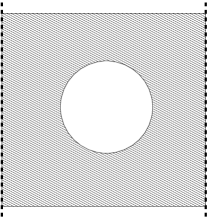
Figure 16: The setup for the computation of the open string decay width as used by Dai and Polchinski [8].

The calculations of Turok et al. [54, 46] include the evaluation of the planar contribution to the self energy. The self energy which is related to the shift of the trajectory has threshold cuts along the positive mass-squared axis, and the discontinuity across the cut gives the decay rate. To determine the values of the decay rates of the asymptotically high-mass states, the method of stationary phase was used to compute the self energy integrals in the upper and lower half planes. It was shown that the decay rates are independent of the endpoint charges, namely the decay of the different gauge representation are the same.

The decay rate of [54] does not agree in general with the one computed by [8], as the former paper finds a decay rate which is not (at leading order) linear in the length $L$ of the string. However, the disagreement disappears in the critical dimension (see the note added in proof in [54]). Since the two methods of calculations used in [8] and [54, 46] are different, the fact that the results agree in the critical dimension is significant. In particular it seems to imply that the impact of the endpoints is not important and indeed the split is a local property. If this conclusion is correct, it is more probable that the massive endpoints of our open strings would not dramatically influence the probability to split.

References

Sakai and Sugimoto [2005]
T. Sakai and S. Sugimoto, “Low energy hadron physics in holographic QCD”,
Prog. Theor. Phys.113 (2005) 843–882,
hep-th/0412141.
Karch and Katz [2002]
A. Karch and E. Katz, “Adding flavor to AdS/CFT”, JHEP 06
(2002) 043,
hep-th/0205236.
Sakai and Sugimoto [2005]
T. Sakai and S. Sugimoto, “More on a holographic dual of QCD”,
hep-th/0507073.
Erdmenger and Kirsch [2004]
J. Erdmenger and I. Kirsch, “Mesons in gauge/gravity dual with large number of
fundamental fields”, JHEP 12 (2004) 025,
hep-th/0408113.
Pando Zayas et al. [2004]
L. A. Pando Zayas, J. Sonnenschein, and D. Vaman, “Regge trajectories
revisited in the gauge/string correspondence”, Nucl. Phys.B682
(2004) 3–44,
hep-th/0311190.
Kruczenski et al. [2005]
M. Kruczenski, L. A. P. Zayas, J. Sonnenschein, and D. Vaman, “Regge
trajectories for mesons in the holographic dual of large- QCD”, JHEP 06 (2005) 046,
hep-th/0410035.
Cotrone et al. [2005]
A. L. Cotrone, L. Martucci, and W. Troost, “String splitting and strong
coupling meson decay”,
hep-th/0511045.
Dai and Polchinski [1989]
J. Dai and J. Polchinski, “The decay of macroscopic fundamental strings”,
Phys. Lett.B220 (1989)
387.
Mitchell and Turok [1987]
D. Mitchell and N. Turok, “Statistical properties of cosmic strings”, Nucl. Phys.B294 (1987)
1138.
Sjöstrand et al. [2003]
T. Sjöstrand, L. Lönnblad, S. Mrenna, and P. Skands, “PYTHIA 6.3:
Physics and manual”,
hep-ph/0308153.
Itzhaki et al. [1998]
N. Itzhaki, J. M. Maldacena, J. Sonnenschein, and S. Yankielowicz,
“Supergravity and the large- limit of theories with sixteen
supercharges”, Phys. Rev.D58 (1998) 046004,
hep-th/9802042.
Witten [1998]
E. Witten, “Anti-de Sitter space, thermal phase transition, and confinement
in gauge theories”, Adv. Theor. Math. Phys.2 (1998) 505,
hep-th/9803131.
Brandhuber et al. [1998]
A. Brandhuber, N. Itzhaki, J. Sonnenschein, and S. Yankielowicz, “Wilson
loops, confinement, and phase transitions in large- gauge theories from
supergravity”, JHEP 06 (1998) 001,
hep-th/9803263.
Kuperstein and Sonnenschein [2004]
S. Kuperstein and J. Sonnenschein, “Non-critical supergravity () and
holography”, JHEP 07 (2004) 049,
hep-th/0403254.
Sakai and Sonnenschein [2003]
T. Sakai and J. Sonnenschein, “Probing flavored mesons of confining gauge
theories by supergravity”, JHEP 09 (2003) 047,
hep-th/0305049.
Babington et al. [2004]
J. Babington, J. Erdmenger, N. J. Evans, Z. Guralnik, and I. Kirsch, “Chiral
symmetry breaking and pions in non-supersymmetric gauge/gravity duals”, Phys. Rev.D69 (2004) 066007,
hep-th/0306018.
Kruczenski et al. [2004]
M. Kruczenski, D. Mateos, R. C. Myers, and D. J. Winters, “Towards a
holographic dual of large- QCD”, JHEP 05 (2004) 041,
hep-th/0311270.
Nastase [2003]
H. Nastase, “On D-D+4 systems, QCD dual and phenomenology”,
hep-th/0305069.
Wang and Hu [2003]
X.-J. Wang and S. Hu, “Intersecting branes and adding flavors to the
Maldacena-Nunez background”, JHEP 09 (2003) 017,
hep-th/0307218.
Nunez et al. [2003]
C. Nunez, A. Paredes, and A. V. Ramallo, “Flavoring the gravity dual of
Yang-Mills with probes”, JHEP 12 (2003) 024,
hep-th/0311201.
Ouyang [2004]
P. Ouyang, “Holomorphic D7-branes and flavored gauge theories”, Nucl. Phys.B699 (2004) 207–225,
hep-th/0311084.
Hong et al. [2004]
S. Hong, S. Yoon, and M. J. Strassler, “Quarkonium from the fifth dimension”,
JHEP 04 (2004) 046,
hep-th/0312071.
Evans and Shock [2004]
N. J. Evans and J. P. Shock, “Chiral dynamics from AdS space”, Phys. Rev.D70 (2004) 046002,
hep-th/0403279.
Bando et al. [2004]
M. Bando, T. Kugo, A. Sugamoto, and S. Terunuma, “Pentaquark baryons in string
theory”, Prog. Theor. Phys.112 (2004) 325–355,
hep-ph/0405259.
Ghoroku and Yahiro [2004]
K. Ghoroku and M. Yahiro, “Chiral symmetry breaking driven by dilaton”, Phys. Lett.B604 (2004) 235–241,
hep-th/0408040.
Arean et al. [2004]
D. Arean, D. E. Crooks, and A. V. Ramallo, “Supersymmetric probes on the
conifold”, JHEP 11 (2004) 035,
hep-th/0408210.
Apreda et al. [2005]
R. Apreda, J. Erdmenger, and N. Evans, “Scalar effective potential for
D7-brane probes which break chiral symmetry”,
hep-th/0509219.
Kruczenski et al. [2003]
M. Kruczenski, D. Mateos, R. C. Myers, and D. J. Winters, “Meson spectroscopy
in AdS/CFT with flavour”, JHEP 07 (2003) 049,
hep-th/0304032.
Son and Stephanov [2004]
D. T. Son and M. A. Stephanov, “QCD and dimensional deconstruction”, Phys. Rev.D69 (2004) 065020,
hep-ph/0304182.
Erlich et al. [2005]
J. Erlich, E. Katz, D. T. Son, and M. A. Stephanov, “QCD and a holographic
model of hadrons”,
hep-ph/0501128.
Da Rold and Pomarol [2005]
L. Da Rold and A. Pomarol, “Chiral symmetry breaking from five dimensional
spaces”, Nucl. Phys.B721 (2005) 79–97,
hep-ph/0501218.
de Teramond and Brodsky [2005]
G. F. de Teramond and S. J. Brodsky, “The hadronic spectrum of a holographic
dual of QCD”, Phys. Rev. Lett.94 (2005) 201601,
hep-th/0501022.
Casero et al. [2005]
R. Casero, A. Paredes, and J. Sonnenschein, “Fundamental matter, meson
spectroscopy and non-critical string/gauge duality”,
hep-th/0510110.
Paredes and Talavera [2005]
A. Paredes and P. Talavera, “Multiflavour excited mesons from the fifth
dimension”, Nucl. Phys.B713 (2005) 438–464,
hep-th/0412260.
Kinar et al. [2000]
Y. Kinar, E. Schreiber, and J. Sonnenschein, “ potential from
strings in curved spacetime – classical results”, Nucl. Phys.B566 (2000) 103–125,
hep-th/9811192.
Wilczek [2004]
F. Wilczek, “Diquarks as inspiration and as objects”,
hep-ph/0409168.
Casher et al. [1979]
A. Casher, H. Neuberger, and S. Nussinov, “Chromoelectric flux tube model of
particle production”, Phys. Rev.D20 (1979)
179–188.
Gurvich [1979]
E. G. Gurvich, “The quark anti-quark pair production mechanism in a quark
jet”, Phys. Lett.B87 (1979)
386–388.
Nayak [2005]
G. C. Nayak, “Non-perturbative quark-antiquark production from a constant
chromo-electric field via the Schwinger mechanism”,
hep-ph/0510052.
Kokoski and Isgur [1987]
R. Kokoski and N. Isgur, “Meson decays by flux tube breaking”, Phys. Rev.D35 (1987)
907.
Sjöstrand [1982]
T. Sjöstrand, “The Lund Monte Carlo for jet fragmentation”, Comp. Phys. Commun.27 (1982)
243.
Andersson et al. [1983]
B. Andersson, G. Gustafson, G. Ingelman, and T. Sjöstrand, “Parton
fragmentation and string dynamics”, Phys. Rep.97 (1983)
31.
Andersson [1998]
B. Andersson, “The Lund model”, Cambridge University Press, 1998.
Ida [1978]
M. Ida, “Relativistic motion of massive quarks joined by a massless string”,
Prog. Theor. Phys.59 (1978)
1661.
Gupta and Rosenzweig [1994]
K. S. Gupta and C. Rosenzweig, “Semiclassical decay of excited string states
on leading regge trajectories”, Phys. Rev.D50 (1994)
3368–3376,
hep-ph/9402263.
Wilkinson et al. [1990]
R. B. Wilkinson, N. Turok, and D. Mitchell, “The decay of highly excited
closed strings”, Nucl. Phys.B332 (1990)
131.
Peeters et al. [2004]
K. Peeters, J. Plefka, and M. Zamaklar, “Splitting spinning strings in
AdS/CFT”, JHEP 11 (2004) 054,
hep-th/0410275.
Peeters et al. [2005]
K. Peeters, J. Plefka, and M. Zamaklar, “Splitting strings and chains”, Found. Phys.53 (2005) 640–646,
hep-th/0501165.
Bigazzi et al. [2005]
F. Bigazzi, A. L. Cotrone, L. Martucci, and L. A. Pando Zayas, “Wilson loop,
Regge trajectory and hadron masses in a Yang-Mills theory from semiclassical
strings”, Phys. Rev.D71 (2005) 066002,
hep-th/0409205.
Karliner et al. [1988]
M. Karliner, I. R. Klebanov, and L. Susskind, “Size and shape of strings”,
Int. J. Mod. Phys.A3 (1988)
1981.
Georgi [1993]
H. Georgi, “The physics of waves”, Prentice-Hall, 1993.
Eidelman et al. [2004]
S. Eidelman et al., “Review of Particle Physics”, Physics Letters B592 (2004) 1.
Frolov and Tseytlin [2002]
S. Frolov and A. A. Tseytlin, “Semiclassical quantization of rotating
superstring in ”, JHEP 06 (2002)
007,
hep-th/0204226.
Mitchell et al. [1989]
D. Mitchell, N. Turok, R. Wilkinson, and P. Jetzer, “The decay of highly
excited open strings”, Nucl. Phys.B315 (1989)
1.
Sundborg [1989]
B. Sundborg, “Selfenergies of massive strings”, Nucl. Phys.B319
(1989)
415–438.
Amano and Tsuchiya [1989]
K. Amano and A. Tsuchiya, “Mass splittings and the finiteness problem of mass
shifts in the type-II superstring at one loop”, Phys. Rev.D39 (1989)
565.