Lab/UFR-HEP0508/GNPHE/0508
Calogero model with Yukawa like interaction

Abstract

We study an extension of one dimensional Calogero model involving strongly coupled and electrically charged particles. Besides Calogero term $\frac{g}{2x^{2}}$, there is an extra factor described by a Yukawa like coupling modeling short distance interactions. Mimicking Calogero analysis and using developments in formal series of the wave function $\Psi\left(x\right)$ factorised as $x^{\epsilon}\Phi\left(x\right)$ with $\epsilon\left(\epsilon-1\right)=g$, we develop a technique to approach the spectrum of the generalized system and show that information on full spectrum is captured by $\Phi\left(x\right)$ and $\Phi^{\prime\prime}\left(x\right)$ at the singular point $x=0$ of the potential. Convergence of $\int dx\left|\Psi\left(x\right)\right|^{2}$ requires $\epsilon>-\frac{1}{2}$ and is shown to be sensitive to the zero mode of $\Phi\left(x\right)$ at $x=0$.

Key words: Hamitonian systems, quantum integrability, Calogero model, Yukawa like potential.

1 Introduction

The study of integrability of hamiltonian systems has been one of the basic tasks during decades as it gives precise informations on classical and quantum dynamics as well as spectrum of the hamiltonians [1, 2]. This analysis has lead to the discovery of several features regarding quantum spectrum of integrable hamiltonian systems [3]-[10]. The familiar examples are given by the remarkable class of integrable low dimensional field models based on both finite dimensional and affine Lie algebras. The study of integrable hamiltonian systems has also shown that there is only a few number of real physical systems that are completely solvable. The usual harmonic oscillator and one dimensional Calogero model as well as extensions [11]-[14] are certainly some of these examples. Despite the variety of methods used to study integrability, one may, roughly speaking, say that the main difficulty in getting exact solutions comes essentially from the fact that the underlying differential equations are non linear coupled relations difficult to solve. Lessons learnt from the study of hamiltonian systems and infinite dimensional symmetries of integrable models let understand that hamiltonian systems may in general be classified into three basic sets: (i) integrable hamiltonian systems where the spectrum of the hamiltonian is exactly determined as in case of Calogero model [3], (ii) quasi-integrable systems where, though not completely determined, the hamiltonian spectrum, obtained by perturbation of exact models, is under control and (iii) remaining others with unknown spectrum.

Motivated by remarkable properties of integrable one dimensional Calogero type interaction [4], we study in this paper the case where Calogero particles are moreover electrically charged and strongly coupled. Coulomb interaction $\frac{1}{\left|x_{i}-x_{j}\right|}$ and strong coupling between pairs of particles $\left\{x_{i},x_{j}\right\}$ are implemented by adjunction to the usual Calogero hamiltonian an extra short distance interaction described by a Yukawa like coupling $\exp\left(-a\left|x_{i}-x_{j}\right|\right)/\left|x_{i}-x_{j}\right|$ where $a$ is the inverse of Debye length $\lambda$. Among our results, we show that for the case of two particles, the discrete spectrum $\left\{E_{n},\Psi_{n}\left(x\right)=x^{\epsilon}\Phi_{n}\left(x\right)\right\}$ of this generalized Calogero system with $\epsilon>-\frac{1}{2}$ is completely determined by the knowledge of the wave factor $\Phi_{n}\left(x\right)$ and $\Phi_{n}^{\prime\prime}\left(x\right)$ at the singular point $x=0$ of the potential. The range $\epsilon>-\frac{1}{2}$ is required by the convergence of $\int dx\left|\Psi_{n}\left(x\right)\right|^{2}$ and is shown to be sensitive to the zero mode of $\Phi_{n}\left(x\right)$ at $x=0$.

The organisation of this paper is as follows: In section 2, we review briefly quantum Calogero model by solving directly the Calogero wave equation for the case of two particles; the case of $N$ particles is straightforward and follows the same lines. Comments regarding this solution are also given; they are used in the interpretation of our generalization. In section 3, we study the extension of Calogero model involving charged and strongly correlated particles described by a Yukawa like interaction. Motivated by similarities with Calogero analysis and inspired from moment technique, we develop a method to approach the discrete spectrum of the generalized Calogero system. In section 4, we give our conclusion and make a discussion regarding some specific limits.

2 $1D$ Calogero model: brief review

One dimensional Calogero model describing the quantum dynamics of two interacting particles, of local coordinates $x_{1}$ and $x_{2}$ and relative position $x=\left(x_{2}-x_{1}\right)/\sqrt{2}$, is governed by the following eigenvalue wave equation $\mathcal{H}\Psi\left(x\right)=E\Psi\left(x\right)$,

$$\left(-\frac{1}{2}\frac{d^{2}}{dx^{2}}+\frac{1}{2}\omega^{2}x^{2}+\frac{g}{2x^{2}}\right)\Psi\left(x\right)=E\Psi\left(x\right),$$ (1)

where to fix the idea we take $x>0$; i.e $x_{2}>x_{1}$. In this relation, $\omega$ is the usual harmonic oscillator frequency and $g$ is the Calogero coupling parameter. To get the discrete spectrum $\left\{E_{n},\Psi_{n}\left(x\right)\right\}$ of this differential equation, it is interesting to use the following direct method which is also valid for the case of a system of $N$ particles. This method relies on solving directly eq(1) and involves three steps each one associated with the factorisation of the field variable $\Psi\left(x\right)$ as $x^{\varepsilon}\Phi\left(x\right)=x^{\varepsilon}P\left(x\right)\exp\left(-\frac{\omega}{2}x^{2}\right)$ for some modulus $\epsilon$. First, set the change $\Psi\left(x\right)=x^{\varepsilon}\Phi\left(x\right)$, which for $\epsilon>0$, reflects just the fact that two classical particles $\left\{x_{1},x_{2}\right\}$ cannot live together at $x_{1}=x_{2}$; the wave function should then vanish; i.e $\Psi\left(0\right)=0$; but $\Phi\left(0\right)\neq 0$. Note that the choice $\epsilon>0$ is not a necessary condition, since quantum mechanically we should rather have,

$$\int_{0}^{\infty}dx\left|\Psi\left(x\right)\right|^{2}<\infty.$$ (2)

As far convergence of this integral is concerned, one should not that there are two sources of possible divergences, one for $x\rightarrow 0$ and the other for $x\rightarrow\infty$. Decomposing eq(2) as $\int_{0}^{y}dx\left|\Psi\left(x\right)\right|^{2}+\int_{y}^{z}dx\left|\Psi\left(x\right)\right|^{2}+\int_{z}^{\infty}dx\left|\Psi\left(x\right)\right|^{2}$ for some small positive number $y$ and a large positive $z$; then using the fact that $\int_{z}^{\infty}dx\left|\Psi\left(x\right)\right|^{2}$ is finite, we will prove later that in the region $0\leq x\leq y$, convergence requires that $\frac{y^{2\varepsilon+1}}{2\varepsilon+1}\left|\Phi\left(0\right)\right|^{2}$ should be finite. By substitution of the change $\Psi\left(x\right)=x^{\varepsilon}\Phi\left(x\right)$ in eq(1), we get the following constraint relation on $\Phi$,

$$\Phi^{\prime\prime}\left(x\right)+\frac{2\varepsilon}{x}\Phi^{\prime}\left(x\right)+\left(2E-\omega^{2}x^{2}\right)\Phi\left(x\right)=0,$$ (3)

which, for a matter of discussion of the solution, we prefer to rewrite it as follows,

$$\Phi^{\prime\prime}\left(x\right)+\frac{2\varepsilon}{x}\Phi^{\prime}\left(x\right)+2\left(E-U\right)\Phi\left(x\right)=0,$$ (4)

with $U\left(x\right)=\omega^{2}x^{2}/2$. Note that the factorisation $\Psi\left(x\right)=x^{\varepsilon}\Phi\left(x\right)$ has been also introduced to fix the power $\epsilon$ in term of Calogero coupling constant $g$ as $g=\varepsilon\left(\varepsilon-1\right)$. This relation follows from the requirement that the change $\Psi=x^{\varepsilon}\Phi$ has to kill the problematic term $\frac{g}{2x^{2}}$ which is one of the two sources of difficulty (non linearity) in the search for exact solution. The other difficulty is treated in the second step which consist to make the local scaling change,

$$\Phi\left(x\right)=P\left(x\right)\exp\left(-\frac{\omega}{2}x^{2}\right),$$ (5)

which for matter of generality, we rewrite it also as $\Phi\left(x\right)=P\left(x\right)\exp\left(-f\left(x\right)\right)$ with $f\left(x\right)=\frac{\omega}{2}x^{2}=\frac{U}{\omega}$. Using this change, we can bring eq(3,4) to the form,

$$P^{\prime\prime}\left(x\right)+\left(\frac{2\varepsilon}{x}-2f^{\prime}\right)P^{\prime}\left(x\right)+\left(2E-2U-2\frac{\varepsilon}{x}f^{\prime}-f^{\prime\prime}+f^{\prime 2}\right)P\left(x\right)=0$$ (6)

By substituting $2U=f^{\prime 2}=\omega^{2}x^{2}$, we discover the following familiar differential equation,

$$P^{\prime\prime}\left(x\right)+\left(\frac{2\varepsilon}{x}-2\omega x\right)P^{\prime}\left(x\right)+\left[2E-\omega\left(2\varepsilon+1\right)\right]P\left(x\right)=0,$$ (7)

where now the coefficient $\left[2E-\omega\left(2\varepsilon+1\right)\right]$ in front of $P\left(x\right)$ is constant. This is a typical equation [15] whose solution is given by a special hypergeometric function which we describe in the next step. Setting $u=\omega x^{2}$ and $P\left(x\right)=L\left(u\right)$ and putting back into above equation, we get the following familiar differential relation,

$$uL^{\prime\prime}\left(u\right)+\left(\frac{2\varepsilon+1}{2}-u\right)L^{\prime}\left(u\right)+\left(\frac{E}{2\omega}-\frac{2\varepsilon+1}{4}\right)L\left(u\right)=0.$$ (8)

This differential equation has a known exact solution given by Laguerre polynomials $L_{n}^{\left(\varepsilon-\frac{1}{2}\right)}\left(u\right)$ provided that the factor $\left(\frac{E}{2\omega}-\frac{2\varepsilon+1}{4}\right)$ is quantized, i.e $\left(\frac{E}{2\omega}-\frac{2\varepsilon+1}{4}\right)=n\in\mathbb{N}$,

$$L_{n}^{\alpha}\left(u\right)=\frac{1}{n!}u^{-\alpha}e^{u}\frac{d^{n}}{du^{n}}\left[u^{\alpha+n}e^{-u}\right],$$ (9)

where the upper index $\alpha$ is a convention notation; it should not be confused with a power. Therefore the discrete spectrum $\left\{E_{n},\Psi_{n}\left(x\right)\right\}$ of quantum Calogero two particle system reads as follows:

$$E_{n}^{cal} = \left(2n+\epsilon+\frac{1}{2}\right)\omega,\qquad n\in\mathbb{N},$$

$$\Psi_{n}\left(x\right) = x^{\epsilon}\exp\left(-\frac{\omega}{2}x^{2}\right)L_{n}^{\left(\varepsilon-\frac{1}{2}\right)}\left(\omega x^{2}\right).$$ (10)

The ground state is given by $\Psi_{0}\left(x\right)=x^{\epsilon}\exp\left(-\frac{\omega}{2}x^{2}\right)$ and $E_{0}^{cal}=\left(\epsilon+\frac{1}{2}\right)\omega$; for $\epsilon=0$ ($g=0$); one recovers the usual spectrum of the ground state for harmonic oscillator.

For later use, it is also interesting to note the three following: (a) First remark that the above solution may be also rewritten in a positive modes series as follows,

$$\mathcal{\Phi}_{n}^{\left(cal\right)}(x;\epsilon,\omega)=\sum_{k=0}^{\infty}C_{n,2k}^{\left(cal\right)}\left(\epsilon,\omega\right)\text{ }x^{2k},$$ (11)

where the expansion coefficients $C_{n,2k}^{\left(cal\right)}\left(\epsilon,\omega\right)$ depending on the coupling moduli,

$$C_{n,2k}^{\left(cal\right)}\left(\epsilon,\omega\right)=\sum_{j=0}^{k}\left(\frac{(-\omega)^{k}C_{n}^{j}}{(k-j)!n!2^{k-j}}\frac{\Gamma(n+\epsilon+\frac{1}{2})}{\Gamma(j+\epsilon+\frac{1}{2})}\right),$$ (12)

with $C_{n}^{j}=n!/j!\left(n-j\right)!$ and where for later use note that $C_{n,0}^{\left(cal\right)}\neq 0$. Though forbidden by the reality condition of total wave $\Psi\left(x\right)$, the manifest discrete symmetry $x\leftrightarrow\left(-x\right)$ of solution (11) is not hazardous; it is a symmetry of the Calogero hamiltonian operator (1). Under the exchange of the position $x_{1}\leftrightarrow x_{2}$, the complex wave function maps as,

$$\Psi\left(x_{1},x_{2}\right)=e^{i\pi\epsilon}\Psi\left(x_{2},x_{1}\right),$$ (13)

showing that, for $\epsilon$ different from even integer, the two particles obey a non trivial statistics. (b) The second thing we want to note is that the coefficients $C_{n,0}^{\left(cal\right)}$ and $C_{n,2}^{\left(cal\right)}$of the series (11) are related as follows,

$$C_{n,2}^{\left(cal\right)}=\frac{-E_{n}^{\left(cal\right)}}{\left(2\epsilon+1\right)}C_{n,0}^{\left(cal\right)}.$$ (14)

From eq(11), one sees that above relation may be also rewritten as $E_{cal}=-\left(2\epsilon+1\right)\frac{\Phi_{cal}^{\prime\prime}\left(0\right)}{\Phi_{cal}\left(0\right)}$. (c) The third thing we want to comment is that quantity $\left(f^{\prime 2}-2\frac{\varepsilon}{x}f^{\prime}-f^{\prime\prime}-2U\right)$ appearing in eq(6) is constant, say equal to $K$. Its solution is obviously given by $U=\frac{\omega^{2}}{2}x^{2},$ $f=\frac{\omega}{2}x^{2}$ and $K=-\left(2\epsilon+1\right)$. Note also if we take $f=\left(\epsilon-1\right)\ln x$, one gets precisely $U=\frac{g}{2x^{2}}$ which is nothing but the first factorisation we have used to absorb Calogero term in the hamiltonian.

3 Calogero model with a Yukawa like potential

In this section, we consider the generalization of previous analysis to the case where the Calogero particles are electrically charged and are moreover strongly correlated. The interaction describing this particular behavior is given by the following Yukawa like potential [16],

$$V_{Yuk}\left(x\right)=\frac{2\alpha}{x}\exp\left(-\frac{x}{\lambda}\right),\qquad x\sqrt{2}=\left|x_{1}-x_{2}\right|,$$ (15)

where $\alpha$ is a coupling constant and $\lambda$ is the Debye length. Note that for the range $x<\lambda$, the two leading terms of $V_{Yuk}\left(x\right)$ are respectively given by the usual Coulombian term $\frac{2\alpha}{x}$ and a constant $\frac{-2\alpha}{\lambda}$. The presence of the constant $\frac{-2\alpha}{\lambda}$ shows that energy spectrum $E$ of this generalized system  should read as $E=E_{cal}-\frac{2\alpha}{\lambda}+$ other contributions coming from Coulomb term and remaining polynomial fluctuations ($\exp\left(-\frac{x}{\lambda}\right)\sim 1-\frac{x}{\lambda}+\frac{1}{2}\left(\frac{x}{\lambda}\right)^{2}$). For $x>\lambda$, the spectrum of the quantum system is mainly given by the usual Calogero one ($\frac{2\alpha}{x}\exp\left(-\frac{x}{\lambda}\right)\sim 0$). The Shrodinger equation describing the quantum dynamics of these interacting particles reads, in local coordinates $x_{1}$ and $x_{2}$, as,

$$\left(-\frac{1}{2}\sum_{i=1}^{2}\frac{\partial^{2}}{\partial x_{i}^{2}}+V\left(x_{1},x_{2}\right)\right)\Psi\left(x_{1},x_{2}\right)=E\Psi\left(x_{1},x_{2}\right),$$ (16)

where $\Psi$ is the total wave function, $V$ is the total translation invariant potential given by,

$$V\left(x\right)=\frac{\omega^{2}}{2}x^{2}+\frac{g}{2x^{2}}+\frac{\sqrt{2}\alpha}{x}\exp\left(-\frac{\sqrt{2}x}{\lambda}\right),$$ (17)

and $E$ is the total energy eigenvalue depending on the potential moduli $\omega,$ $g,$ $\alpha$ and $\lambda$. Note that, like for Calogero system, transformation generated by space scale dilatation $x\rightarrow\zeta x,$ maps the hamiltonian $\mathcal{H}$ as follows $\mathcal{H}\rightarrow\zeta^{-2}\mathcal{H}$ provided that couplings are mapped as $\omega\rightarrow\zeta^{-2}\omega,$ $g\rightarrow g,$ $\alpha\rightarrow\zeta^{-1}\alpha$ and $\lambda\rightarrow\zeta\lambda$. Note moreover that the limit $\alpha$ small is also equivalent to large values of the relative distance $x$ with respect to the Debye length $\lambda$ ($x>>\lambda$). In this region, the additional Yukawa like interaction $\frac{\sqrt{2}\alpha}{x}\exp\left(-\frac{\sqrt{2}}{\lambda}x\right)$ may be neglected.

To get the discrete spectrum $\left\{E_{n},\Psi_{n}\left(x\right)\right\}$ of the wave equation eqs(16,17), we shall follow the Calogero method outlined in previous section and the moment technique to be introduced later on. Using classical properties of the wave function and translation invariance ($x_{i}\rightarrow x_{i}+cst$), we can thus decompose $\Psi\left(x\right)$ in three factors as before $\Psi\left(x\right)=x^{\varepsilon}\exp\left(-\frac{\omega}{2}x^{2}\right)P\left(x\right)$ where a priori $\epsilon$ is positive; but quantum effects requires that it should be as $\epsilon>-\frac{1}{2}$ as we show later, see also eq(2) and [17]. In the first step, the factorisation of $\Psi$ reads as follows $\Psi\left(x\right)=x^{\epsilon}\mathcal{\Phi}(x)$. Like in Calogero analysis, this factorisation is also used to kill the non linear term $\frac{g}{x^{2}}$ by making an appropriate choice of $\epsilon$ parameter ($\epsilon=\epsilon\left(g\right)$). Finding $\Psi\left(x\right)$ is then equivalent to determining the $\epsilon$ parameter in terms of potential moduli and the unknown function $\mathcal{\Phi}(x)$. Substituting $\Psi^{\prime\prime}=x^{\epsilon}\mathcal{\Phi}^{\prime\prime}+2\epsilon x^{\epsilon-1}\mathcal{\Phi}^{\prime}+\epsilon(\epsilon-1)x^{\epsilon-2}\mathcal{\Phi}$ in eq(16), Schrödinger equation becomes,

$$\mathcal{\Phi}^{\prime\prime}+\frac{2\epsilon}{x}\mathcal{\Phi}^{\prime}+\left[\frac{\epsilon(\epsilon-1)-g}{x^{2}}-\omega^{2}x^{2}-\frac{2\sqrt{2}\alpha}{x}\exp\left(\frac{-x\sqrt{2}}{\lambda}\right)+2E\right]\mathcal{\Phi}=0.$$ (18)

This is a second order differential equation with non constant coefficients which, as we know, its solution isn’t a simple matter. However, eq(18) may be simplified a little bit by working, like in Calogero model, in a special region of the coupling constant moduli space;

$$\epsilon(\epsilon-1)-g=0\text{,\qquad}\alpha,\lambda\text{ free moduli}.$$ (19)

Note that $g=g\left(\epsilon\right)$ is quadratic function in $\epsilon$ and so it has two zeros namely $\epsilon_{-}\left(g=0\right)=0$ and $\epsilon_{+}\left(g=0\right)=1$, see also figure,

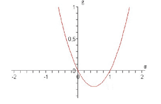
Figure 1: This figure describes the variation of Calogero coupling constant ${\small\mathit{g}}$ in term of the statistical parameter $\epsilon$. As one sees there is two regions for Calogero coupling g, attractive and repulsive. In the interface ${\small\mathit{g=0}}$, we have two solutions  $\left(\epsilon_{-},g\right)=\left(0,0\right)$  and $\left(\epsilon_{+},g\right)=\left(1,0\right)$,  which, by eq(13), shows that they correspond to Bose and Fermi statistics respectively. For generic values of g, we have the two branches $\epsilon_{\pm}\left(g\right)=\frac{1\pm\sqrt{1+4g}}{2}$.

As $\epsilon$ is the basic parameter in this analysis, it is then interesting to express it like $\epsilon=\epsilon\left(g\right)$; but this leads however to two possible solutions $\epsilon_{\pm}\left(g\right)$ given by,

$$\epsilon_{-}\left(g\right)=\frac{1-\sqrt{1+4g}}{2},\qquad\epsilon_{+}\left(g\right)=\frac{1+\sqrt{1+4g}}{2}.$$ (20)

Generally speaking, one should distinguish between these two cases; however this not necessary since these values are related as $\epsilon_{+}\left(g\right)+\epsilon_{-}\left(g\right)=1$. One derives the quantum spectrum for one of the cases, say $\epsilon=\epsilon_{+}\left(g\right)$, then deduces the other one by using the identity $\epsilon_{-}=1-\epsilon_{+}$. The second step is to factor $\Phi$ as $\Phi\left(x\right)=P\left(x\right)\exp\left(-\frac{\omega}{2}x^{2}\right)$ in order to absorb the harmonic term $\omega^{2}x^{2}$. By substitution, the previous equation becomes

$$P^{\prime\prime}+\left(\frac{2\epsilon}{x}-2x\omega\right)P^{\prime}+\left(2E-\left(2\epsilon+1\right)\omega-\frac{2\sqrt{2}\alpha}{x}e^{\frac{-x\sqrt{2}}{\lambda}}\right)P=0,$$ (21)

where obviously $\epsilon$ stands for $\epsilon_{\pm}\left(g\right)=\frac{1\pm\sqrt{1+4g}}{2}$. Strictly speaking we have two wave equations to solve and then two discrete spectrum to get; we shall refer to them as $\left\{\Psi_{n}^{\pm},\text{ }E_{n}^{\pm}\right\}$. Note moreover that the two above factorisation of the field variable $\Psi\left(x\right)$ implies, amongst others, the two following: (i) The first change of variables fixes the parameter $\epsilon$ as $\epsilon_{\pm}=\frac{1\pm\sqrt{1+4g}}{2}$ whose reality property requires that $g\geq-\frac{1}{4}$ showing that there are various phases, an attractive one associated to the moduli space $-\frac{1}{4}\leq g<0$ and which may be interpreted as a confining phase, two repulsive ones given by $g>0$ with $-\frac{1}{2}<\epsilon_{-}\leq 0$ and $\epsilon_{+}\geq 1$ and finally two interfaces associated with the points $\left(\epsilon_{-},g\right)=\left(0,0\right)$ and $\left(\epsilon_{+},g\right)=\left(1,0\right)$. Note that quantum mechanically, the classical argument $\Psi\left(x\right)=0$ for $x=0$ leading to $\epsilon>0$ is not a quantum principle. The right condition is to require rather that $\Psi\left(x\right)$ is a Hilbert space wave function with a convergent integral $\int dx\left|\Psi\left(x\right)\right|^{2}<\infty$. Following [16], wave functions such as $\Psi\left(x\right)=x^{\epsilon}\Phi\left(x\right),$ with $\epsilon>\frac{-1}{2},$ are also Hilbert space solutions despite the apparent divergence at $x=0$. This feature is a typical quantum mechanical property which may be derived in several manners; one of which is the elaborated one developed in [16] using canonical operator formalism; a second one is given by the direct method to be developed below and leading to eq(24). To have a quick idea on the rule behind this $\epsilon$ shift to left, we present here below a naive way to see it. The argument relies on considering eq(21) and requires vanishing of fundamental energy for arbitrary values of relative position $x$. This is a typical feature dictated by renormalisability of quantum systems and allow to redefine energy origin by absorbing the constant term. Recall that in quantum mechanics, the fundamental energy constant term captures quantum effects and is one of the sources of divergences. In canonical quantization for instance, this term has some thing to do with operators normal ordering and is absorbed in the renormalisation process shifting energy as $E\geq 0$. For our concern, it is enough to look at boundaries of the system ($\left|x\right|\rightarrow\infty$) where Yukawa like interaction may be ignored. The corresponding energy positivity condition $E\geq 0$ is then the same as in Calogero case and reads as $\frac{E}{2\omega}\geq\frac{2\varepsilon+1}{4}$ or equivalently $2\epsilon+1>0$. In general, one can prove that for the case of $N$ particles, this condition extends as $N\epsilon+1>0$ showing that we should have $\epsilon>\frac{-1}{N}$. In what follow we shall give an other way to deal with this quantum shift. (ii) The second factorisation of the wave function tells us that as far as moduli space of coupling constants is concerned, one may also consider the moduli space region where the term $\frac{\sqrt{2}\alpha}{x}\exp\left(\frac{-x\sqrt{2}}{\lambda}\right)$ can be treated as a perturbation around Calogero potential ($\frac{\alpha}{\lambda}<<1$). There, the spectrum $\left\{E_{n}\left(\epsilon,\omega,\alpha,\lambda\right),\mathcal{P}_{n}\left(x;\epsilon,\omega,\alpha,\lambda\right)\right\}$ we are looking for should reduce to Calogero one, plus fluctuations as shown below;

$$\mathcal{P}_{n}\left(x;\epsilon,\omega,\alpha,\lambda\right) = \mathcal{P}_{n}^{\left(cal\right)}\left(x;\epsilon,\omega\right)+\mathcal{O}\left(\alpha,\frac{1}{\lambda}\right),$$

$$E_{n}\left(\epsilon,\alpha,\lambda\right) = E_{n}^{\left(cal\right)}\left(\epsilon,\omega\right)+\mathcal{O}\left(\alpha,\frac{1}{\lambda}\right),$$ (22)

where $\mathcal{P}_{n}^{\left(cal\right)}(x;\epsilon,\omega)$ and $E_{n}^{\left(cal\right)}$ are the exact Calogero spectrum eq(10); see also conclusion section. The normalisation condition of the total wave function $\Psi$, which, by using the factorisation $\Psi\left(x\right)=x^{\epsilon}P\left(x\right)\exp\left(-\frac{\omega}{2}x^{2}\right)$, reads as,

$$\int_{0}^{\infty}\left|\Psi\left(x\right)\right|^{2}dx=\int_{0}^{\infty}x^{2\epsilon}P^{2}\left(x\right)e^{-\omega x^{2}}dx,\qquad\epsilon>-\frac{1}{2},$$ (23)

requires convergence of the integral. For $x=\infty$, such condition is ensured provided that $x^{2\epsilon}P^{2}\left(x\right)<e^{-\omega x^{2}}$ and for $x=0$, the quantity $\frac{x^{2\epsilon+1}}{2\epsilon+1}P^{2}\left(0\right)$ should be finite. Both these conditions are fulfilled for Laguerre polynomials associated with Calogero model. In the case where Yukawa like coupling are implemented, the function $P\left(x\right)$ is no longer polynomial but has expansion type $\sum_{s\geq 0}p_{s}x^{s}$ involving positive modes only; that is with a good behavior near $x=0$. Under this assumption we can prove that eq(23) converges as well for the range $\epsilon>-\frac{1}{2}$ exactly as in Calogero system. Let us give some details on the proof. First note there are two sources for possible divergences of eq(23), one at $x=+\infty$ and the other at $x=0$. At infinity, Yukawa like potential $\frac{1}{x}e^{-ax}$ is negligible and the system is mainly the Calogero one where, as noted before, solutions are known for the range $\epsilon>-\frac{1}{2}$. In this case $P\left(x\right)$ is a polynomial eq(11) and its convergence is ensured by the gaussian factor whatever the value of $\epsilon$ is. At $x=0$ however, the situation is some how subtle; we have $e^{-\omega x^{2}}\sim 1-\omega x^{2}+O\left(x^{4}\right)$ and so a possible divergence may come from low modes of the expansion of $P\left(x\right)$ which may be approximated in this region as $p_{0}+p_{1}x+O\left(x^{2}\right)$ independently on whether $P\left(x\right)$ is a polynom or not; the only requirement is that $P\left(x\right)$ should have positive modes only. Therefore, we have $x^{2\epsilon}P^{2}\left(x\right)e^{-\omega x^{2}}\sim p_{0}^{2}x^{2\epsilon}+2p_{0}p_{1}x^{2\epsilon+1}+O\left(x^{2\epsilon+2}\right)$, which diverges for $\epsilon\leq\frac{-1}{2}$ since,

$$\int\left|\Psi\left(x\right)\right|^{2}dx\simeq\frac{p_{0}^{2}}{2\epsilon+1}x^{2\epsilon+1}+\frac{2p_{0}p_{1}}{2\epsilon+2}x^{2\epsilon+2}+\frac{p_{1}^{2}-p_{0}^{2}\omega}{2\epsilon+3}x^{2\epsilon+3}+O\left(x^{2\epsilon+4}\right).$$ (24)

At $2\epsilon+1=0$, one has a logarithmic divergence; it corresponds to a critical point describing collapsing particles as interpreted in [16]. For $2\epsilon+2=0,$ one has both linear and logarithmic divergences. However in the range $\epsilon>\frac{-1}{2}$ the situation is healthy like in Calogero model. Note that convergence of $\int\left|\Psi\left(x\right)\right|^{2}dx$ is also sensitive to the values of the modes $p_{s}$. For $p_{0}=0$ for instance, even the logarithmic divergence at $\epsilon=\frac{-1}{2}$ disappear and, as one sees on eq(24), is shifted to the moduli space point $\epsilon=\frac{-3}{2}$.

Theorem 1

:  
(a) The discrete energy eigenvalues $E_{n}$ of generalized Calogero system with electrically charged particle and strongly correlated described, in addition to Calogero term, by a Yukawa like interaction eq(18) are given by

$$E_{n}\left(\epsilon,\alpha,\lambda\right)=-\left(2\epsilon+1\right)\frac{\Phi_{n}^{\prime\prime}\left(0\right)}{\Phi_{n}\left(0\right)}+f\left(\alpha,\lambda\right)$$ (25)

where $\Phi_{n}\left(0\right)$ and $\Phi_{n}^{\prime\prime}\left(0\right)$ are the values of the wave function $\Phi\left(x\right)$ and its second derivative at $x=0$ and where $f\left(\alpha,\lambda\right)$ is equal to $\frac{2\alpha\left(\lambda\alpha-\epsilon\right)}{\epsilon\lambda}$.
(b) The total wave functions $\Psi_{n}\left(x\right)=x^{\epsilon}\Phi_{n}\left(x\right)$ of this generalized Calogero system is completely determined up to the knowledge of the field (zero mode) values $\Phi_{n}\left(x=0\right)$ and $\Phi_{n}^{\prime\prime}\left(x=0\right)$.

Having in mind the method of solving standard Calogero wave equation presented in section 2 and convergence of (23) for $P\left(x\right)$ with an expansion type $\sum_{s\geq 0}p_{s}x^{s}$ involving positive modes, one may proceed ahead to establish this theorem by mimicking the same method. The idea is to start from eq(18) which we rewrite as,

$$\mathcal{\Phi}_{n}^{\prime\prime}+\frac{2\epsilon}{x}\mathcal{\Phi}_{n}^{\prime}+\left[2E_{n}-\omega^{2}x^{2}-\frac{2\sqrt{2}\alpha}{x}\exp\left(\frac{-x\sqrt{2}}{\lambda}\right)\right]\mathcal{\Phi}_{n} = 0,$$

$$P^{\prime\prime}\left(x\right)+\left(\frac{2\varepsilon}{x}-2\omega x\right)P^{\prime}\left(x\right)+\left(2E-\left(2\epsilon+1\right)\omega-U\right)P\left(x\right) = 0,$$ (26)

where $U=\frac{2\sqrt{2}\alpha}{x}e^{\frac{-x\sqrt{2}}{\lambda}}$ and try to put it in a form type (7-8).

To prove the theorem, we shall develop a method inspired from the solution (11) and an expansion of the wave function as a formal series. The key idea may be summarized as follows: first use the feature $\int_{-\infty}^{\infty}dx\left|\Psi_{n}\left(x\right)\right|^{2}<\infty$ eq(23) and the factorisation $\Psi_{n}\left(x\right)=x^{\epsilon}P_{n}\exp\left(-\frac{\omega}{2}x^{2}\right)$ to build the wave functions $\Psi_{n}$. Second benefit from known properties of Calogero wave function, in particular its development as a series (11,12) with positive modes which we suppose also valid in presence of Yukawa like interaction,

$$\Phi_{n}\left(x\right)=\sum_{r\geq 0}C_{n,r}\left(\epsilon,\omega,\alpha,\lambda\right)\text{ }x^{r},\qquad\epsilon>0,$$ (27)

where the $C_{n,k}$ coefficients, depending on the coupling moduli, are the new unknown quantities which have to be determined. This means that, like $\Psi_{n}^{\left(cal\right)}\left(x\right)=x^{\epsilon}\Phi^{\left(cal\right)}\left(x\right)$, the wave $\Psi_{n}\left(x\right)=x^{\epsilon}\Phi_{n}\left(x\right)$ may be expanded in a formal series as,

$$\Psi_{n}\left(x\right)=\sum_{r\geq 0}C_{n,r}\left(\epsilon,\omega,\alpha,\lambda\right)\text{ }x^{r+\epsilon}.$$ (28)

To that purpose, note that in a distribution sense, the integral $\int_{-1}^{1}\frac{1}{m+1}x^{m}dx=\int_{-1}^{1}d\left(x^{m+1}\right)$ is usually equal to zero except for the case $m=-1$ where the integral is different from zero. Using this property, which may be thought of as a real version of Cauchy theorem of complex analysis, we can inverse eq(28) as follows,

$$C_{n,l}\left(\epsilon,\omega,\alpha,\lambda\right)=\int_{-1}^{1}x^{-l-1}\Phi_{n}\left(x\right)=\frac{1}{l!}\Phi^{\left(l\right)}\left(0\right),\qquad l\geq 0.$$ (29)

To get the explicit expression of the new variables $C_{n,l}\left(\epsilon,\omega,\alpha,\lambda\right)$, we start from the differential equation,

$$x^{2}\mathcal{\Phi}_{n}^{\prime\prime}+2\epsilon\left(x\mathcal{\Phi}_{n}^{\prime}\right)+\left[2E_{n}x^{2}-\omega^{2}x^{4}-2\sqrt{2}\alpha x\exp\left(\frac{-x\sqrt{2}}{\lambda}\right)\right]\mathcal{\Phi}_{n}=0.$$ (30)

Putting the expansion $\mathcal{\Phi}_{n}\left(x\right)=\sum_{k=0}^{\infty}C_{n,k}$ $x^{k}$ back into eq(30) and using the development $\exp\left(\frac{-x\sqrt{2}}{\lambda}\right),$ namely $\sum_{m=0}^{\infty}\frac{\left(-\right)^{m}2^{\frac{m}{2}}}{\lambda^{m}m!}x^{m}$, we get after term rearranging the following algebraic equation,

$$\sum_{k\geq 0}A_{n,k}\text{ }x^{k}=0$$ (31)

where the first four $A_{n,k}$ coefficients are as $A_{n,0}=\left[\epsilon(\epsilon-1)-g\right]C_{n,0}$, $A_{n,1}=\left(2\epsilon+\epsilon(\epsilon-1)-g\right)C_{n,1}-2\sqrt{2}\alpha C_{n,0}$ together with

$$A_{n,2} = \left(2\left(2\epsilon+1\right)+\epsilon(\epsilon-1)-g\right)C_{n,2}-2\left[\sqrt{2}\alpha C_{n,1}-\left(E_{n}+\frac{2\alpha}{\lambda}\right)C_{n,0}\right],$$ (32)

$$A_{n,3} = \left(3\left(2\epsilon+2\right)+\epsilon(\epsilon-1)-g\right)C_{n,3}-2\left[\sqrt{2}\alpha C_{n,2}-\left(E_{n}+\frac{2\alpha}{\lambda}\right)C_{n,1}+\frac{\sqrt{2}\alpha}{\lambda^{2}}C_{n,0}\right].$$

and the remaining others ($k\geq 4$) read as $A_{n,k}=\left[k\left(2\epsilon+k-1\right)+\epsilon(\epsilon-1)-g\right]C_{n,k}-D_{n,k}$, with $D_{n,k}$s given by,

$$D_{n,k}=2\alpha\sum_{m=0}^{k-1}\frac{\left(-\right)^{m}2^{\frac{m+1}{2}}}{m!\lambda^{m}}C_{n,k-m-1}+\omega^{2}C_{n,k-4}-2E_{n}C_{n,k-2}$$ (33)

The solution of eq(31) for arbitrary $x$ is obtained by requiring the vanishing of the $A_{n,k}$ coefficients which give in turn the following recurrent constraint eqs on the $C_{n,k}$ functions,

$$0 = \left[\epsilon(\epsilon-1)-g\right]C_{n,0},$$

$$C_{n,1} = \frac{2\alpha\sqrt{2}}{2\epsilon+\epsilon(\epsilon-1)-g}C_{n,0},$$

$$C_{n,2} = \frac{2\left[\sqrt{2}\alpha C_{n,1}-\left(E_{n}+\frac{2\alpha}{\lambda}\right)C_{n,0}\right]}{2\left(2\epsilon+1\right)+\epsilon(\epsilon-1)-g},$$ (34)

$$C_{n,3} = \frac{2\sqrt{2}\alpha C_{n,2}-2\left(E_{n}+\frac{2\alpha}{\lambda}\right)C_{n,1}+2\frac{\sqrt{2}\alpha}{\lambda^{2}}C_{n,0}}{3\left(\epsilon+1\right)+\epsilon(\epsilon-1)-g},$$

and for $k\geq 4,$

$$C_{n,k}=\frac{2\alpha\sum_{m=0}^{k-1}\frac{\left(-\right)^{m}2^{\frac{m+1}{2}}}{m!\lambda^{m}}C_{n,k-m-1}+\omega^{2}C_{n,k-4}-2E_{n}C_{n,k-2}}{k(2\epsilon+k-1)+\epsilon(\epsilon-1)-g}$$ (35)

From these recurrent relations, one sees that in the case $\epsilon\neq 0$ the elements of the infinite set $\left\{C_{n,k}\right\}$ are all of them function of $C_{n,0}$, the zero mode of the expansion (28), and the energy $E_{n}$. Notice that in the case $\epsilon=0$, one is left with Yukawa like model since classically there is no Calogero interaction. In this situation and using the relations $A_{n,0}=\left[\epsilon(\epsilon-1)-g\right]C_{n,0}$, $A_{n,1}=\left(2\epsilon+\epsilon(\epsilon-1)-g\right)C_{n,1}-2\sqrt{2}\alpha C_{n,0}$ together with $A_{n,2}$ and $A_{n,3}$ given by eqs(32), we have either $C_{n,0}\neq 0$; but $\alpha=0$ or $C_{n,0}=0$ and $\alpha\neq 0$. In the second case, one should have $C_{n,1}\neq 0$ otherwise the wave function vanishes. Non trivial solution requires $C_{n,0}\neq 0$; the first equation of (34) fixes then the Calogero $g$ coupling constant as in the case of absence of Yukawa like coupling,

$$\epsilon(\epsilon-1)=g.$$ (36)

Putting this relation back into above eqs(34,35), we get the following reduced constraint eqs,

$$C_{n,1} = \frac{\alpha\sqrt{2}}{\epsilon}C_{n,0},$$

$$C_{n,2} = \frac{C_{n,0}}{2\epsilon+1}\left(\frac{2\alpha^{2}}{\epsilon}-\frac{2\alpha}{\lambda}-E\right),$$ (37)

$$C_{n,3} = \frac{\sqrt{2}\alpha C_{n,0}}{3\left(\epsilon+1\right)}\left[\frac{2\alpha^{2}}{\epsilon\left(2\epsilon+1\right)}-\frac{\left(3\epsilon+1\right)\left(E_{n}+\frac{2\alpha}{\lambda}\right)}{\epsilon\left(2\epsilon+1\right)}+\frac{1}{\lambda^{2}}\right],$$

together with the following recurrent relations,

$$C_{n,k}=\frac{2\alpha\sum_{m=0}^{k-1}\frac{\left(-\right)^{m}2^{\frac{m+1}{2}}}{m!\lambda^{m}}C_{n,k-m-1}+\omega^{2}C_{n,k-4}-2E_{n}C_{n,k-2}}{k(2\epsilon+k-1)}.$$ (38)

From eqs(37), one sees that for $\epsilon\neq 0$ one can express the energy $E_{n}$ in terms of the coefficients $C_{n,0}$ and $C_{n,2}$ as shown below,

$$E_{n}=\left(\frac{2\alpha^{2}}{\epsilon}-\frac{2\alpha}{\lambda}\right)-\left(2\epsilon+1\right)\frac{C_{n,2}}{C_{n,0}}.$$ (39)

The knowledge of $C_{n,0}$ and $C_{n,2}$ fixes then completely the spectrum $\left\{\Psi_{n}\left(x\right),E_{n}\right\}$; but we have no exact way to determine $C_{n,0}$ and $C_{n,2}$; except the use of approximation methods. This is the case where the correlation between particles are strong enough ($x<<\lambda$) so that the Yukawa like coupling may be interpreted as a perturbation with respect to Calogero interaction. In this limit, the ratio $\frac{C_{n,2}}{C_{n,0}}$ may be approximated by eq(14) and consequently the approximated energy reads as $E_{n}=\left(\frac{2\alpha^{2}}{\epsilon}-\frac{2\alpha}{\lambda}\right)+E_{n}^{cal}$ with $\epsilon\neq 0$. As one sees $\Delta E_{n}=\Delta E_{n}^{cal}\sim\Delta E_{n}^{osc}$ whatever positive integer $n$ is; it would be interesting to check this behaviour by other methods. Progress in this matter will be exposed in a future occasion. Note finally that the case $\epsilon=0$ with non trivial wave function requires $C_{n,0}=0$, but $C_{n,1}\neq 0$ and the previous energy relation get replaced by $2\alpha^{2}-\frac{2\alpha}{\lambda}-3\frac{C_{n,3}}{C_{n,1}}$.

4 Conclusion and discussions

In this paper, we have studied an extension of one dimensional Calogero model involving electrically charged particles with strong correlations. These couplings are described, in addition to Calogero potential $\frac{g}{2x^{2}}$, by a Yukawa like interaction $V_{Yuk}\left(x\right)=\frac{2\alpha}{x}\exp\left(-\frac{x}{\lambda}\right),$ $x\sqrt{2}=\left|x_{1}-x_{2}\right|$. Though this system is not completely integrable; we have shown that its discrete spectrum $\left\{\Psi_{n}\left(x\right)=x^{\epsilon}\Phi_{n}\left(x\right),E_{n}\right\}$, $\epsilon>\frac{-1}{2},$ may be totally determined up to fixing the value of the wave factor $\Phi_{n}\left(x\right)$ and $\Phi_{n}^{\prime\prime}\left(x\right)$ at the singularity $x=0$ of the potential; that is the zero mode $C_{n,0}$ and the second one $C_{n,2}$ of the wave function expansion eq(28). The quantum condition $\epsilon>\frac{-1}{2}$ is shown to be intimately related with the non zero value $\Phi_{n}\left(0\right)$; see eq(24). In the case of Calogero model, the modes $C_{n,0}^{cal}$, $C_{n,2}^{cal}$ and energy $E_{n}^{cal}$ are all of them fixed by a remarkable property of confluent hypergeometric functions which are solution of eq(8) and which, for discrete spectrum, reduces to Laguerre polynomials. In this study, we do not have a similar property due to the presence of highly non linear potential interactions ($\exp\left(-\frac{x}{\lambda}\right)$). We have focused on the case of two identical particles $\left\{x_{1},x_{2}\right\}$; but this is just a matter of simplicity. Our analysis extends also to the case of a generic number $N$ of identical particles $\left\{x_{1},...,x_{N}\right\}$. There, the wave function $\Psi$ depends on the $\frac{N\left(N-1\right)}{2}$ relative positions $x_{ij}=x_{i}-x_{j}$ ($\Psi\left(x\right)=\left(\Pi_{i,j}x_{ij}\right)^{\epsilon}\Phi\left(x_{12},...,x_{N-1,N}\right)$) and the expansion of the factor $\Phi\left(x_{12},...,x_{N-1,N}\right)$ follows the same lines as for the case of two particles considered here.

In the end, we would like to add two comments. First note that for $g=\epsilon\left(\epsilon-1\right)$, one should distinguish the moduli space regions: (i) $-\frac{1}{2}<\epsilon\leq 0$, (ii) $0\leq\epsilon\leq 1$ and (iii) $\epsilon>1$. Moreover solving $g=\epsilon\left(\epsilon-1\right)$ as $\epsilon_{\pm}\left(g\right)$ eqs(20), one sees that the corresponding spectrum $\left\{\Psi_{n}^{\pm},E_{n}^{\pm}\right\}$ may be split into $\left\{\Psi_{2k+1}^{+},E_{2k+1}^{+}\right\}$ and $\left\{\Psi_{2k}^{-},E_{2k}^{-}\right\}$ with $k$ positive integer. This splitting has a particularly interesting interpretation in the moduli space region $g$ and $\alpha$ go to zero. Physically speaking, this corresponds to large $x$ where the two potential components $\frac{g}{x^{2}}$ and $\frac{\alpha}{\left|x\right|}e^{-\frac{\left|x\right|}{\lambda}}$ are negligible with respect to harmonic interaction $\frac{\omega^{2}}{2}x^{2}$. In this limit, the discrete spectrum $\left\{\Psi_{n}^{\pm},E_{n}^{\pm}\right\}$ should then tend to the usual spectrum $\left\{\Psi_{n}^{\left(osc\right)},E_{n}^{\left(osc\right)}\right\}$ of one dimensional harmonic oscillator. Setting $g=\alpha=0$ in eq(10), one gets $E_{n}\left(\epsilon=0,\alpha=0\right)=E_{n}^{cal}\left(\epsilon=0\right)=\left(2n+\frac{1}{2}\right)\omega,$ $n\in\mathbb{N}$; which at first sight seems not reproducing the full energy spectrum of the harmonic oscillator that we recall here $E_{n}^{\left(osc\right)}=\left(n+\frac{1}{2}\right)\omega,$ $n\in\mathbb{N}$. The naive relation between $E_{n}^{cal}\left(\epsilon=0\right)$ and $E_{n}^{\left(osc\right)}$ reads as,

$$E_{n}^{cal}\left(\epsilon=0\right)=E_{2n}^{\left(osc\right)},$$ (40)

and shows that apparently there are missing terms associated with the odd integer modes $E_{2n+1}^{\left(osc\right)}$. In fact there is no contradiction here since we have not implemented the full picture for the limit $g=0$. In this case, one should distinguish two sectors $\epsilon_{+}=1$, $g=0$ and $\epsilon_{-}=0$, $g=0$ whose respective energies $E_{n}^{\left(+,cal\right)}\left(g=0\right)$ and $E_{n}^{\left(-,cal\right)}\left(g=0\right)$ are given by $\lim_{g\rightarrow 0}\left[\left(2n+1\right)+\frac{1}{2}\sqrt{1+4g}\right]\omega=\left[\left(2n+1\right)+\frac{1}{2}\right]\omega$ and $\lim_{g\rightarrow 0}\left[\left(2n+1\right)-\frac{1}{2}\sqrt{1+4g}\right]\omega=\left[2n+\frac{1}{2}\right]\omega$. They read in terms of $E_{n}^{\left(osc\right)}$ as follows,

$$E_{n}^{\left(+,cal\right)}\left(g=0\right)=E_{2n+1}^{\left(osc\right)},\qquad E_{n}^{\left(-,cal\right)}\left(g=0\right)=E_{2n}^{\left(osc\right)}.$$ (41)

As one sees Calogero interaction splits harmonic oscillator energies into two blocks $E_{2n+1}^{\left(osc\right)}$ and $E_{2n}^{\left(osc\right)}$ with a global separation $\left|E_{2n+1}^{\left(osc\right)}-E_{2n}^{\left(osc\right)}\right|=\omega$ whatever the integer $n$ is. This is a remarkable feature which should deserve more investigation. The second comment concerns the low mode structure of wave functions $\Psi_{n}^{\pm}$ obtained from eqs(28, 34-35) by implementation of eqs(20). In the limit $\epsilon_{+1}=1,$ $g=0$ and the case $C_{n,0}^{+}\neq 0$,  we have for leading terms $C_{n,1}^{+}=\alpha\sqrt{2}C_{n,0}^{+}$, $C_{n,2}^{+}=\frac{C_{n,0}^{+}}{3}(2\alpha^{2}-\frac{2\alpha}{\lambda}-E_{n}^{+})$, $C_{n,3}^{+}=\frac{C_{n,0}^{+}}{6}(\frac{\sqrt{2}\alpha}{3}(2\alpha^{2}-\frac{2\alpha}{\lambda}-E_{n}^{+})-\sqrt{2}\alpha(E_{n}^{+}+\frac{2\alpha}{\lambda})+\frac{\sqrt{2}\alpha}{\lambda^{2}})$ together with the following modes $C_{n,k}^{+}=\frac{1}{k(k+1)}(2\alpha\sum_{m=0}^{k-1}\frac{(-)^{m}2^{\frac{m+1}{2}}}{m!\lambda^{m}}C_{n,k-m-1}^{+}+\omega^{2}C_{n,k-4}^{+}-2E_{n}^{+}C_{n,k-2}^{+}$) for $k\geq 4$. In the case $\epsilon_{-}=0,$ $g=0$; but $C_{n,0}^{-}=0$ and $C_{n,1}^{-}\neq 0$, we have $C_{n,2}^{-}=\alpha\sqrt{2}C_{n,1}^{-},$ $C_{n,3}^{-}=\frac{C_{n,1}^{-}}{3}(2\alpha^{2}-\frac{2\alpha}{\lambda}-E_{n}^{-})$, $C_{n,4}^{-}=\frac{C_{n,1}^{-}}{6}(\frac{\sqrt{2}\alpha}{3}(2\alpha^{2}-\frac{2\alpha}{\lambda}-E_{n}^{-})-\sqrt{2}\alpha(E_{n}^{-}+\frac{2\alpha}{\lambda})+\frac{\sqrt{2}\alpha}{\lambda^{2}})$ and for $k\geq 4$, $C_{n,k}^{-}=\frac{1}{k(k-1)}(2\alpha\sum_{m=0}^{k-1}\frac{(-)^{m}2^{\frac{m+1}{2}}}{m!\lambda^{m}}C_{n,k-m-1}^{-}+\omega^{2}C_{n,k-4}^{-}-2E_{n}^{-}C_{n,k-2}^{-}$). Note that the modes in the two cases are related as $C_{n,k}^{+}(\epsilon_{+}=1)C_{n,1}^{-}(\epsilon_{-}=0)=C_{n,k+1}^{-}(\epsilon_{-}=0)C_{n,0}^{+}(\epsilon_{+}=1)$. At last note that near $x=0$, the wave function $\Psi_{n}\left(x\right)=x^{\epsilon}\Phi_{n}\left(x\right)$ behaves as $x^{\epsilon}\left(C_{n,0}+C_{n,1}x+O\left(x^{2}\right)\right)$. In the case where the leading modes are as $C_{n,0}=0$ and $C_{n,1}\neq 0$, all happens as if $\epsilon$ is shifted as $\widetilde{\epsilon}=\epsilon+1$ and $\widetilde{C}_{n,0}=C_{n,1}$.

Acknowledgement 2

The authors would like to thank prof A Intissar and A El Rhalami for discussions. This research work is supported by the program Protars III D12/25, CNRST.

References

- [1] F.Calogero, J.Math.Phys. 10 (1969) 2191, 2197, J.Math.Phys. 12 (1971) 419
- [2] B.Sutherland, J.Math.Phys. 12 (1971) 246.
- [3] M.A.Olshanetsky, A.M.Perelomov, Phys.Rept.71(1981)313.
- [4] E.H. Saidi, M.B. Sedra, A. Serhani, Phys.Lett.B353:209-212,1995; E.H Saidi, M.B Sedra, Int.J.Mod.Phys.A9:891-913,1994; M.Caselle, U.Magnea, Phys.Rept394 (2004)41
- [5] T.Guhr, H.Kohler, J.Math.Phys.43,(2002)2741
- [6] H.J.Stoeckmann, J.Phys.A Math.Gen.37 (2004)137; B.D.Simons, P.A.Lee, B.L.Altshuler, Phys.Rev.Lett. 70 (1993)4122.
- [7] G.W.Gibbons, P.K.Townsend, Phys.Lett. B454, 187(1999).
- [8] E. Sahraoui, E.H. Saidi, Class.Quant.Grav.16:1605-1615,1999 ; J.Gomis, A.Kapustin, JHEP 0406(2004)002.
- [9] A.P.Polychronakos, Phys.Rev.Lett. 69 (1992) 703.
- [10] M.Olshanetsky, Universality of Calogero-Moser model, J.Nonlin.Math.Phys. 12 (2005) S522-S534, nlin.SI/0410013
- [11] S. Meljanac, A. Samsarov, Matrix oscillator and Calogero-type models, Phys.Lett. B600 (2004) 179-184, hep-th/0408241,
- [12] Reiho Sakamoto, Jun’ichi Shiraishi, Daniel Arnaudon, Luc Frappat, Eric Ragoucy, Correspondence between conformal field theory and Calogero-Sutherland model, Nucl.Phys. B704 (2005) 490-509, hep-th/0407267,
- [13] A.Gorsky, N.Nekrasov, Hamiltonian systems of Calogero type and two dimensional Yang-Mills, Nucl.Phys. B414 (1994) 213-238 theoryhep-th/9304047,
- [14] Francesco Calogero, A solvable many-body problem in the plane, J. Nonlinear Math. Phys. 5 (1998), no. 3, 289-293, math-ph/9807037
- [15] G.Palma and U.Raff, the one-dimensional harmonic oscillator in the presence of a dipole-like interaction, Am.J.Phys. 71 (2003) 247
- [16] Xiang-Qian Luo, Yong-Yao Li, Helmut Kroger, Bound States and Critical behavior of the Yukawa potential, hep-ph/0407258
- [17] Velimir Bardek, Larisa Jonke, Stjepan Meljanac, Marijan Milekovic, Phys.Lett.B 531 (2002) 311, hep-th/0107053.