On the $S$-matrix renormalization in effective theories

Abstract

This is the 5-th paper in the series devoted to explicit formulating of the rules needed to manage an effective field theory of strong interactions in $S$-matrix sector. We discuss the principles of constructing the meaningful perturbation series and formulate two basic ones: uniformity and summability. Relying on these principles one obtains the bootstrap conditions which restrict the allowed values of the physical (observable) parameters appearing in the extended perturbation scheme built for a given localizable effective theory. The renormalization prescriptions needed to fix the finite parts of counterterms in such a scheme can be divided into two subsets: minimal — needed to fix the S-matrix, and non-minimal — for eventual calculation of Green functions; in this paper we consider only the minimal one. In particular, it is shown that in theories with the amplitudes which asymptotic behavior is governed by known Regge intercepts, the system of independent renormalization conditions only contains those fixing the counterterm vertices with $n\leq 3$ lines, while other prescriptions are determined by self-consistency requirements. Moreover, the prescriptions for $n\leq 3$ cannot be taken arbitrary: an infinite number of bootstrap conditions should be respected. The concept of localizability, introduced and explained in this article, is closely connected with the notion of resonance in the framework of perturbative QFT. We discuss this point and, finally, compare the corner stones of our approach with the philosophy known as “analytic $S$-matrix”.

I Introduction

This paper, together with the previous one AVVV2 , is aimed to form the philosophical and theoretical base for calculations proposed in VVV –POMI and to outline the ways for further analysis, therefore it is natural to review first the material presented in those publications.

We are interested in constructing a self-consistent perturbation technique for the infinite component effective field theories of strong interactions. We work with Dyson’s scheme, because it is the only known way to combine Lorentz invariance, unitarity and cluster decomposition principle with postulates of quantum mechanics. Thus, the problems we have to do with include an infinite number of graphs to be summed up at each loop order and the problem of ordering the required renormalization conditions, since in such a theory one needs to fix an infinite number of parameters to be able to calculate amplitudes. In AVVV1 it has been shown that already the requirement of summability of tree graphs — the existence of well-defined tree level amplitudes — leads to strong limitations on the possible values of coupling constants of a theory. However, in those articles some theoretical statements, like meromorphy and polynomial boundedness of the tree level amplitude, were taken as postulates and only some general arguments in their favor were given. With these assumptions it became possible to obtain the system of bootstrap equations for masses and coupling constants of $\pi\pi$ and $\pi K$ resonances in nice agreement with experimental data. The main tool used to derive them was the Cauchy expansion, based on the celebrated Cauchy integral formula, which represents the tree level amplitude as a well defined series in a given domain of the space of kinematical variables.

In subsequent publications we fill some gaps left in the previous analysis and discuss new concepts. Thus, in POMI (see also MENU ) we suggest the notion of minimal parametrization and in AVVV2 the corresponding reduction theorem is proven. This theorem explains why it is sufficient to consider only the minimal (“on-shell-surviving”) vertices at each loop order of the perturbation theory — the fact implicitly used in AVVV1 to parameterize amplitudes. Besides, in POMI we briefly discuss what we call the localizability requirement — the philosophy which, in particular, serves as background for the requirements of polynomial boundedness and meromorphy of tree level amplitudes. Since the last point was not explained clear enough, we address it in this paper.

We start with summing up the main results of previous publication AVVV2 in Sec. II. Continuing the logic line of that article we consider the extended perturbation scheme based on the interaction Hamiltonian which, along with the fields that describe true asymptotic states, contains also auxiliary fields of fictitious unstable particles — resonances. In Sec. III we formulate two mathematical principles: asymptotic uniformity and summability, which create a base for constructing the meaningful perturbation series in such effective theory. Further, in Sec. IV we briefly discuss the mathematical tool which allows us to present the finite loop order amplitudes as convergent functional series. This technique is exploited in Secs. V–VI, where we demonstrate how the requirement of crossing symmetry gives rise to the system of bootstrap conditions and analyze the renormalization procedure. The results of these two Sections are generalized in Sec. VII, where phenomenological constraints are imposed and the renormalization prescriptions are explicitly written; besides, it is shown there that the bootstrap conditions obtained at any loop order can be treated as the relations between physical observables, which justify the legitimacy of our preceding analysis of experimental data AVVV1 ; MENU ; Talks .

The connection between the extended perturbation scheme and the localizable initial theory (based on the Hamiltonian constructed solely from the fields of true asymptotic states) is outlined in Sec. VIII which, along with Sec. III, is the central one in this article. In particular, we discuss here a (rather hypothetic) step-by-step process of localization and explain our usage of the term “strong interaction”. The localization process requires introducing auxiliary free fields. The physical interpretation of those fields is given in Sec. IX where we discuss the meaning of the terms “mass” and “width” as the resonance classification parameters.

At last, the Section X is devoted to comparative analysis of the effective scattering theory philosophy with respect to that of analytic $S$-matrix.

II Classification of the parameters: a brief review

For the following discussion it is essential to recall the results obtained in AVVV2 . Referring to the analysis presented there we attempt to be not too rigorous trying, instead, to make a picture clear.

We say that the field theory is effective if the interaction Hamiltonian in the interaction picture contains all the monomials consistent with a given algebraic (linear) symmetry. Effective scattering theory is just the effective field theory only used to compute the $S$-matrix, while the calculation of Green functions is not implied. In particular, only the $S$-matrix elements should be renormalized.

The fields of stable particles and resonances of arbitrary high spin are present in effective Hamiltonian and every vertex is dotted by the corresponding coupling constant. Therefore we are forced to deal with an infinite set of parameters. By construction, the effective theory is renormalizable but, to make use of this property, one needs an infinite number of renormalization prescriptions. This looks impractical until certain regularity reducing the number of independent prescriptions, possibly up to some basic set, is found. As shown in AVVV2 , the $S$-matrix in effective theory only depends upon a certain set of parameters, which we called the resultant parameters of various levels (or loop orders) $l$. The value $l=0$ labels the tree-level parameters, $l=1$ — one-loop level ones, and so on.

The parametrization implies the use of renormalized perturbation theory (see, e.g. Vasiliev2 ; Renorm ; Peskin ), so the interaction Hamiltonian is written as a sum of basic one plus counterterms:

$${\cal H}_{\rm int}={\cal H}_{\rm b}+{\cal H}_{\rm ct}\ .$$

The coupling constants in ${\cal H}_{\rm b}$ are the physical ones, while each counterterm contributes starting from appropriate loop order. The resultant parameters of order $l=0$ include mass parameters and certain infinite polylinear combinations of the Hamiltonian coupling constants with coefficients depending on masses. The $l$-th level resultant parameters ${v}^{(l)}_{\cdots}$ with $l\geq 1$ contain also the items depending on counterterm couplings of orders $l^{\prime}\leq l$. In fact, it is the new counterterms arising at each new loop order that makes this classification convenient in perturbative calculations.

The construction of resultant parameters implies transition to the minimal parametrization, in which every $S$-matrix graph is built of minimal propagators and minimal vertices. The numerator of the minimal propagator is just a covariant spin sum considered as a function of four independent components of momentum. The essence of the term “minimal” when relates to a scalar function is that the latter looks similar on and off the mass shell, and when relates to a tensor structure, is that it does not vanish when dotted by relevant wave function. The central object is the minimal effective vertex.

To explain what it is, we start from the basic Hamiltonian (without counterterms). Let us single out all its items constructed from a given set of, say, $n$ normally ordered field operators with quantum numbers collectively referred to as $i_{1},\ldots,i_{n}$. These items differ from each other by the Hamiltonian coupling constants, by the number of derivatives and/or, possibly, by their matrix structure due to fermions or a linear symmetry group. Now, consider a momentum space matrix element of the (formal) infinite sum of all these terms. This matrix element should be calculated on the mass shell, presented in a Lorentz-covariant form and considered as a function of $4(n-1)$ independent components of particle momenta $p_{k}^{\mu}$ (four-momentum conservation $\delta$-function is retained, but on-shell restriction is relaxed). The wave functions should be crossed out. The resulting structure we call as $n$-leg minimal effective vertex of the Hamiltonian level. Every such vertex $V^{({\scriptscriptstyle\cal H})}$ presents a finite sum

$$V^{({\scriptscriptstyle\cal H})}_{\ldots}(i_{1},\ldots,i_{n};\,p_{1},\ldots,p_{n})$$

$$=\delta(\Sigma p_{k})\;\sum_{a}T_{\ldots}^{a}V_{a}^{({\scriptscriptstyle\cal H})\,i_{1}\ldots i_{n}}(\nu_{1},\ldots,\nu_{3n-10})\ ,$$ (1)

of tensor/matrix structures $T^{a}_{\ldots}$ dotted by scalar formfactors $V_{a}^{({\scriptscriptstyle\cal H})}$ linear in Hamiltonian coupling constants, each formfactor being a formal power series in relevant scalar kinematical variables $\nu_{1},\ldots,\nu_{3n-10}$ (the amount of independent scalars formed of $p_{k}^{\mu}$ that can survive on-shell is $3n-10$):

$$V_{a}^{({\scriptscriptstyle\cal H})\,i_{1}\ldots i_{n}}(\ldots)=\sum_{r_{1},\ldots,r_{d}=0}^{\infty}g^{(a,{\scriptscriptstyle\cal H})\,i_{1}\ldots i_{n}}_{r_{1}\ldots r_{d}}\;\nu_{1}^{r_{1}}\ldots\nu_{d}^{r_{d}}\ ,$$

$$d=3n-10;$$

here $g^{(a,{\scriptscriptstyle\cal H})\,i_{1}\ldots i_{n}}_{r_{1}\ldots r_{d}}$ stand for linear combinations of the Hamiltonian couplings.

We use the term “minimal vertex of the Hamiltonian level” (not effective) to denote any separate contribution to the above series — a momentum space vertex produced by the basic Hamiltonian which does not alter on-shell when dotted by the wave functions of external particles. Except the trivial cases like $\phi^{4}$, a Hamiltonian term (like, e.g. $\phi^{2}\partial_{\mu}\phi\partial^{\mu}\phi$) gives rise to both minimal and non-minimal vertices, that is why the notion of minimality makes sense in momentum space only. It is also sensible to the choice of variables $\nu_{k}$, thereby in actual calculations one should fix this choice which, however, is not essential here.

Minimal vertices of tree and higher levels can be constructed after all the amplitude graphs are subjected to the reduction procedure AVVV2 . In this process some of propagators disappear being cancelled, e.g., by $(p^{2}-M^{2})$ factors from non-minimal vertices. The two vertices connected by such propagator flow together to form a single secondary vertex, like e.g. in Fig 1.

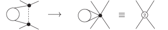
Figure 1: Example of graph reduction: the dotted propagator is cancelled by non-minimal (vanishing on-shell, or when multiplied by the wave function forming the propagator numerator) structure coming from one of the vertices. Two initial vertices merge to form a secondary vertex, 2-loop bubble-like structure is absorbed in the coupling of new 2-nd level vertex.

To preserve loop counting, we assign to this new vertex the level index equal to the loop order of the initial structure reduced (contracted) to form the vertex plus the loop order of bubble-like structure got attached to this vertex after the reduction of all graphs is completed (Fig. 2).

Figure 2: Vertices of the levels $l=1,2$ pictured via Hamiltonian vertices: bubbles just rescale couplings and increase the level index.

For example, if two Hamiltonian vertices were connected with one another by one $(l-k)$-loop self-energy subgraph and, in addition, by the $k$ simple propagators, the reduction of the latter ones leads to appearing of a new — secondary — vertex of the $l$-th level: see e.g. Fig. 1, where $k=1$ and $l=2$. Further, if one of the initial vertices was, say, 1-loop counterterm, then the level assigned to the secondary vertex is $l+1$, and so on, so that the initial loop order is kept. The idea, of course, is that self-closed lines do not alter the tensor/matrix structure of the vertex, only rescaling the vertex coupling (the regularization is implied). Thus it is natural to treat the vertex together with bubbles as a new single vertex, where a new coupling is given by the product of the two (or more) initial ones, times whatever bubbles give. However, since there are hidden loops, this new vertex should not appear in calculations until the needed loop order is reached.

In AVVV2 we have shown that after full reduction is done, all the amplitude graphs are expressed via the minimal propagators and minimal vertices, some of them being the secondary vertices of various levels. All of them are minimal in a sense that they do not change their Lorentz-covariant form when put on mass shell and multiplied by the relevant wave functions. All bubble-like structures disappear forming minimal vertices of higher levels.

Now, we define the $0$-th (tree) level minimal effective vertex as that of the Hamiltonian level plus the sum of all $0$-th level secondary vertices with the same external legs. Clearly, the most general tensor structure of the vertex is defined by the external legs only, therefore the tensor structure of the tree level minimal effective vertex is the same as that of the Hamiltonian level vertex (1). However, due to secondary vertices, the formfactors $V_{a}^{(0)\,i_{1}\ldots i_{n}}$ are not anymore linear in Hamiltonian couplings.

The $l$-th level minimal effective vertex with the same set of external legs is just a sum of all $l$-th level minimal vertices with those legs, without adding the $l$-th level minimal effective counterterm vertex with the same legs. As we just mentioned, the presence of bubbles does not change the tensor structure of the effective vertex, it only affects the coefficients of scalar formfactors. These latter coefficients (eventually supplied with the index $l$) are called the $l$-th level minimal parameters.

Consider now a process involving a given set of external particles. Along with other graphs, the renormalized $l$-th loop order amplitude of this process acquires contributions from both $l$-th level minimal effective vertex and $l$-th level minimal effective counterterm with the same set of external lines. Since both vertices have the same tensor structure, we can finally combine them into a single effective vertex, which we call the resultant vertex of the $l$-th level. Simply speaking, we allow awkward vertices with bubbles and those came from the reduction of non-minimal elements of graphs produced by the initial Feynman rules to be absorbed by the relevant counterterms of the corresponding loop order and consider the resulting combination as a single item. Analogous to minimal parameters, the $l$-th level resultant parameters (couplings) are the coefficients in formal power series representing relevant formfactors or, in general, any other set of independent parameters describing the resultant vertex. They are, of course, the functions of initial Hamiltonian couplings. However the latter functional dependence is not of interest anymore: we are not going to fix any of couplings in the initial Hamiltonian. Rather, we will prefer to operate with minimal or resultant parameters directly. The simplest case is the 3-, 2- and eventual 1-leg resultant vertices. One can easily check, that when put on shell and multiplied by relevant wave functions, the 1- and 2-leg vertices do not depend on external momenta, while those with 3 legs can only depend on it through the tensor structures like $p^{\mu}$ or $\gamma^{\mu}$. Hence, the formfactors in corresponding minimal effective (and resultant) vertices are reduced to constants.

Reduction technique introduced in AVVV2 allows one to show that any amplitude graph of loop order $L$ can always be presented as a sum of graphs built of minimal propagators and the minimal vertices of the levels $l\leq L$. In turn, the full (renormalized) sum of such $L$-th order graphs describing certain scattering process can be re-expressed solely in terms of minimal propagators and the resultant vertices ${V_{res}^{(l)}}_{\cdots}$ with level indices $l\leq L$. Therefore, as long as the $S$-matrix is considered, the only building blocks we need in the Feynman rules are the resultant vertices and the minimal propagators.

The special convenience of dealing with the set of resultant parameters is that it is full and its members are independent. It is full in the sense that no other constants are needed to describe the renormalized $S$-matrix elements of the $L$-th loop order but the resultant parameters with $l\leq L$. They are independent in the sense that taking account of the higher loop order $l>L$ graphs leaves the structure of the lower level $l\leq L$ parameters unchanged. The reason for this is of course a freedom in the counterterm couplings which we consider independent at this stage. Thus, two resultant vertices $V^{(l_{1})}$ and $V^{(l_{2})}$ with the same external lines but of different levels $l_{1}$ and $l_{2}$ are described by precisely the same tensor structures, but the coefficients in power series (in the same set of variables) — the resultant parameters — do not depend on each other, which is indicated by different level indices. Besides, by the very construction, the resultant parameters of the same level are independent, as far as we consider independent all the coupling constants in the effective Hamiltonian.

However, there is one thing, unpleasant from the technical point of view, that happens during the reduction. As above, suppose that one works with regularized expressions. Before the reduction one could think about all the amplitude graphs at any loop order as being finite: the counterterms were adjusted in a way that all subdivergencies for each given graph are cancelled when regularization is removed. As it is clearly seen, the reduction is nothing but rearrangement of parameters within the graphs of a given loop order — it does not change the values of $S$-matrix elements. Imagine, however, that some graph had a subgraph with the divergency proportional to $p^{2}-M^{2}$, where $p$ and $M$ are the momenta and mass of a particle on corresponding external (w.r.t. the subgraph) leg. Before the reduction this subdivergency had been removed by the relevant explicitly drawn counterterm vertex of the form

$$-C(p^{2}-M^{2})+\ldots\ ,$$

where $C$ possesses exactly the same singular behavior w.r.t. regulator as the relevant part of the subgraph. But during the reduction the situation changes. Due to non-minimal structure, $(p^{2}-M^{2})$, the corresponding propagator disappears from the graph and the non-minimal counterterm gets absorbed by the new (secondary) vertex. As a result, we may have a subgraph with divergency proportional to $(p^{2}-M^{2})$ and no explicit counterterm to kill it. Instead, one of new couplings acquire singular behavior so that the $S$-matrix remains finite. This is technically inconvenient, because one is then forced to keep working with regularization until all the amplitude graphs of a given loop order are calculated.

Looking for remedy, one may find convenient to re-introduce some non-minimal counterterms after the reduction is done. This, in turn, may require renormalization prescriptions fixing the relevant non-minimal parameters. Since, as stressed above, the $S$-matrix does not depend on the latter, the only thing one needs to take care of is that the chosen values of non-minimal quantities do not fall in contradiction with various self-consistency relations. We shall treat this technical problem in forthcoming publication. In this paper we just assume that it is solved in one way or another (see also the discussion in Sec. VI and Appendix C).

It is now clear that renormalization prescriptions (RP’s) required to calculate the finite $S$-matrix are of two types. The first type RP’s restrict the off-shell behavior of subgraphs. These prescriptions play no role in fixing the on-shell value of the graph itself; they are only needed to make convenient the intermediate steps of amplitude calculations and, in principle, would be required to get finite Green functions. We do not consider them in this paper. In contrast, the second set of RP’s (called below as minimal) fixes the finite parts of counterterm constants contained in resultant parameters, which determine the value of each $S$-matrix element. Therefore the first step towards reducing the required number of independent RP’s is to study the structure of this latter set.

There are certain subtleties in the usage of resultant vertices for constructing the amplitude. First, the only possible tadpoles are the $1$-leg resultant vertices which, as explained in Sec. VII, can be safely dropped. Next, as mentioned above, the self-closed lines are also not present anymore being absorbed in resultant vertices. It makes no sense to picture explicitly those bubbles, because the resultant couplings are independent parameters of a theory. Therefore, due to “hidden” loops present in vertices with levels $l\geq 1$, the true loop order of a graph $L_{true}$ may differ from the number of explicitly drawn loops $L_{expl}$. To keep the right loop order, we have to take account of the level index $l_{i}$ of each resultant vertex $V_{i}^{(l_{i})}$. The true loop order is then given by the number of explicitly drawn loops plus the sum of levels of the vertices used to construct the graph under consideration:

$$L_{true}=L_{expl}+\sum_{vertices}l_{i}\ .$$ (2)

We can now sum up the results of AVVV2 discussed in this Section in a form of instruction. To construct the $L$-loop contribution to the amplitude of a given process in the framework of effective scattering theory, one needs to:

1) Use the system of Feynman rules only containing the minimal propagators and minimal effective (resultant) vertices of the levels $l\leq L$.

2) Construct all the graphs with $L_{expl}\leq L$ explicit loops with no bubbles involved and take account of the relevant symmetry coefficients. Below (Sec. VIII) we argue that there is no need in calculating amplitudes of the processes with external lines corresponding to resonances.

3) Pick up and sum all the graphs respecting relation (2) with $L_{true}=L$.

We will need these results in Sec. V–VII to explore the structure of minimal RP’s needed to fix the physical content of effective scattering theory. But first we shall formulate two principles which we use as the basis for constructing the well-defined finite loop order amplitudes.

III Basic principles of constructing the perturbation series

In a sense, the argumentation in this Section and in Sec. VIII below is inspired by the philosophy originally developed by Krylov and Bogoliubov Bogoliubov for nonlinear oscillation theory. It is concerned with perturbation series with singular behavior and allows one to group the items in a way that the summation procedure acquires meaning. In this spirit we specify certain requirements for the Dyson’s type series arising in the strong interaction effective theories.

First of all one needs a parameter to put the terms of perturbation series in certain order. Since the effective Hamiltonian involves an infinite number of coupling constants, the conventional logic (weak coupling or, the same, small perturbation) does not work, especially in strong interaction physics. That is why it is commonly accepted to classify the terms in perturbation series according to the (true) number of loops in Feynman graphs (see, e.g., Coleman ).

However, in effective theories the problem of meaning of the loop series expansion (is it convergent? asymptotic?…) is even more intricate than in conventional renormalizable theories. Indeed, in this case each item of the loop expansion, in turn, presents an infinite unordered sum of graphs. This is because the interaction Hamiltonian is a formal sum of all possible monomials constructed from the field operators and their derivatives of arbitrary high degree and order. The problem of strong convergence of such operator series is not simple, if ever meaningful in the framework of perturbation theory. Instead, below we formulate two conditions of weak convergence for the functional series for $S$-matrix elements of a given loop order.

One of the most important requirements which we make use of when constructing the meaningful items of the Dyson perturbation series is that of polynomial boundedness. Namely, the full sum of $S$-matrix graphs with given set of external lines and fixed number $L$ of loops must be polynomially bounded in every pair energy at fixed values of the other kinematical variables. There are two basic reasons for imposing this limitation. First, from general postulates of quantum field theory (see, e.g., axioms ) it follows that the full (non-perturbative) amplitude must be a polynomially bounded function of its variables. Second, the experiment shows that this is quite a reasonable requirement. Since we never fit data with non-perturbative expressions for the amplitude, it is natural to impose the polynomial boundedness requirement on a sum of terms up to any fixed loop order and, hence, on the sum of terms of each order. Similar argument also works with respect to the bounding polynomial degrees. To avoid unnecessary mutual contractions between different terms of the loop series, we attract the following asymptotic uniformity requirement: the degree of the bounding polynomial which specifies the asymptotics of a given loop order amplitude must be equal to that specifying the asymptotics of the full (non-perturbative) amplitude of the process under consideration. Surely, this latter degree may depend on the type of the process as well as on the values of the variables kept fixed.

The condition of asymptotic uniformity (or, simply, uniformity) is concerned with the asymptotic behavior of the total contribution at some fixed loop order, but does not tells us how the unordered infinite sum of graphs with the same number of loops (and, of course, describing the same process) can be converted into the well-defined summable functional series. To solve the latter problem we rely upon another general principle which we call summability requirement. It is formulated as follows: in every sufficiently small domain of the complex space of kinematical variables there must exist an appropriate order of summation of the formal series of contributions coming from the graphs with given number of loops, such that the reorganized series converges. Altogether, these series must define a unique analytic function with only those singularities that are present in individual graphs.

At first glance, the summability requirement may seem somewhat artificial. This is not true. There are certain mathematical and field-theoretical reasons for taking it as the guiding principle that provides a possibility to manage infinite formal sums of graphs in a way allowing to avoid inconsistencies. It is, actually, both the summability and uniformity principles that allow us to use the Cauchy formula to obtain well defined expression for the amplitude of a given loop order. This will be demonstrated many times in the rest of the article.

We would like to stress that the requirements of uniformity and summability are nothing but independent subsidiary conditions fixing the type of perturbation scheme which we only work with. Surely, there is no guarantee that on this way one can construct the most general expressions for the $S$-matrix elements in effective theory. Nevertheless, there is a hope to construct at least meaningful ones presented by the Dyson’s type perturbation series only containing the well-defined items.

IV The Cauchy formula in hyper-layers

Applying the famous Cauchy integral formula to the scattering amplitude is a basic tool of the analytic $S$-matrix approach and it is very well treated in the literature. We also use this tool but in a way essentially different from the conventional one.

First, we apply the Cauchy formula to the finite loop order amplitudes. Second, being armed with the polynomial boundedness principle discussed in the previous Section, we pay special attention to the convergency of resulting series of integrals. Basically, we treat the Cauchy integral as the tool to put in order the so far unordered scope of Feynman graphs of a given loop order in a way that the resulting series converge and, therefore, make sense. This turns out especially useful when we need to express the amplitude of a given loop order in terms of resultant vertices and for deriving bootstrap equations for the physical parameters. For use in the rest of the article and for future references we shall thus outline the main steps of the Cauchy integral formula application.

Consider a function $f(z,{\bf x})$ analytic in the complex variable $z$ and smoothly depending on a set of parameters ${\bf x}\equiv\{x_{i}\}$. Suppose further that when ${\bf x}\in D$, where $D$ is a small domain in the parameter space, this function has only a finite number of singular points in every finite domain of the complex-$z$ plane. In Fig. 3

Figure 3: System of embedded contours on the complex-$z$ plane.

it is shown the geography of singular points $s_{k}\equiv s_{k}(\bf x)$, $k=\pm 1,\pm 2,\ldots$, typical for the finite loop order scattering amplitudes in quantum field theory. Both left and right singular points are enumerated in order of increasing modulo. Note that the cuts are drawn in unconventional way — just to simplify the figure. If the point $s_{k}$ corresponds to the pole type singularity there is no need in a cut, but its presence makes no influence on the following discussion.

Let us recall the definition of the polynomial boundedness property adjusted for the case of many variables AVVV1 . Consider the system of closed embedded contours $C(i)\equiv C_{-m_{i},n_{i}}$ (Fig. 3) such that every $C(i)$ surrounds $C(i-1)$ and does not cross the singular points. We say that the function $f(z,{\bf x})$ is $N$-bounded in the hyper-layer $B_{x}\{z\in{\bf C},\,{\bf x}\in D\}$ if there is an infinite system of contours $C(i)$, $i=1,2,\ldots$, and an integer $N$ such that

$$\max_{{\bf x}\in D;\ z\in C(i)}{\left|\frac{f(z,{\bf x})}{z^{N+1}}\right|}\longrightarrow 0$$ (3)

when $i\rightarrow\infty$. The minimal $N$ (possibly, negative), which provides the correctness of the uniform (in $x$) estimate (3), we call the degree of bounding polynomial in the layer $B_{x}$.

Instead of the precise definition given above, one can just keep in mind the rough condition, more “strong”: $f({\bf x},z)=o(|z|^{N+1})$ for all ${\bf x}\in D$ and large $|z|$, except small vicinities of singularities.

Condition (3) makes it natural to apply the Cauchy’s integral formula for the function $f(z,{\bf x})/z^{N+1}$ on the closed contour formed by $C(i)$ (except small segments crossing the cuts), the corresponding parts of the contours $C_{k}$, $k=-m_{i},...,-1,1,...,n_{i}$, surrounding cuts, and a small circle around the origin (the last one is not drawn in Fig. 3). In the limit $i\to\infty$ one obtains:

$$f(z,{\bf x})=\sum\limits_{n=0}^{N}\frac{1}{n!}f^{(n)}(0,{\bf x})z^{n}$$

$$+\ \frac{z^{N+1}}{2\pi i}\sum\limits_{k=-\infty}^{+\infty}\;\oint\limits_{C_{k}}\frac{f(\xi,{\bf x})}{{\xi}^{N+1}(\xi-z)}\;dz\ ,$$ (4)

with $f^{(n)}(z,{\bf x})\equiv\partial^{n}/\partial z^{n}\,f(z,{\bf x})$. It is essential to perform the last summation in order of increasing modulo of the singularities $s_{k}$ which the contours $C_{k}$ are drawn around. The equation (4) provides a mathematically correct form of the result. If the number of singular points is infinite, every contour integral on the right side should be considered as a single term of the series. The mentioned above order of summation provides a guarantee of the uniform (in both $z$ and ${\bf x}$) convergence of the series. The formula (4) plays the key role in the renormalization programme discussed below.

If the function $f$ represents the tree level amplitude, the summability principle formulated in Sec. III does not permit any brunch cut, because only the pole type singularities appear in tree level graphs. Hence, all the contours $C_{k}$ are reduced to circles around poles and all the integrals in Eq. (4) can be expressed via the relevant residues. It is this way that the Cauchy forms introduced in AVVV1 arise. For future reference we discuss this case in Appendix A.

V Minimal prescriptions 1: tentative consideration

The reason to construct resultant parameters shortly discussed in Sec. II is to single out the renormalization prescriptions (RP’s) needed to calculate scattering amplitudes perturbatively. In turn, the results of Secs. III and IV give a hand in forming the expressions for given loop order amplitude in terms of resultant parameters. The following three Sections demonstrate how all this works together in explicit amplitude calculations. Very important result is formulated in Sec. VII. Namely, it is shown that, under certain assumptions suggested by phenomenology, in the effective scattering theory of strong interactions one only needs to know those minimal RP’s which fix the resultant vertices with 1, 2 and 3 external legs. The other resultant couplings turn out to be fixed by certain self-consistency conditions. To show the origin of these conditions we discuss below a simple example illustrating the main idea of our renormalization procedure.

Consider an elastic scattering process

$$a(p_{1})+b(k_{1})\to a(p_{2})+b(k_{2})\ ,$$ (5)

where we took both $a$ and $b$ particles to be spinless: this considerably simplifies the purely technical details without changing the logical line of the analysis.

Along with the conventional kinematical variables $s=(k_{1}+p_{1})^{2}$, $t=(k_{1}-k_{2})^{2}$ and $u=(k_{1}-p_{2})^{2}$, we introduce three equivalent pairs of independent ones:

$$(x,{\nu}_{x}),\quad x=s,t,u;$$ (6)

$${\rm where}\;\;{\nu}_{s}=u-t,\;{\nu}_{t}=s-u,\;{\nu}_{u}=t-s.$$

The pair $(x,{\nu}_{x})$ provides a natural coordinate system in 3-dimensional (one complex and one real coordinate) hyper-layer $B_{x}\{\nu_{x}\in{\bf C};\;x\in{\bf R};\;x\sim 0\}$, while the pair $(x,{\rm Re}\;{\nu}_{x})$ does the same in the band parallel to the corresponding side $x=0$ of the Mandelstam triangle: Fig. 4.

Figure 4: Disposition of the bands $B_{x}$ (bounded by dotted lines) and intersection domains $D_{x}$ (hatched) $(x=s,t,u)$.

Let us suppose that in $B_{t}\{\nu_{t}\in{\bf C};\;t\in{\bf R},\;t\sim 0\}$ the full (non-perturbative) amplitude of the process (5) is described by the 0-bounded function $f(\nu_{t},t)$ ($N_{t}\leq 0$). It is quite a typical experimental situation in hadron physics; in the end of this Section we discuss more involved cases. According to the uniformity principle (Sec. III), we have to construct the perturbation series

$$f({\nu}_{t},t)=\sum\limits_{l=0}^{\infty}f_{l}({\nu}_{t},t)$$

in such a way that each full sum $f_{l}(...)$ of the $l$-th loop order graphs also presents the 0-bounded function in $B_{t}$. Hence, the relation (4) in this layer reads

$$f_{l}({\nu}_{t},\;t)=f_{l}(0,t)+\frac{{\nu}_{t}}{2\pi i}\sum\limits_{k=-\infty}^{+\infty}\;\oint\limits_{C_{k}(t)}\frac{f_{l}(\xi,t)}{{\xi}(\xi-{\nu}_{t})}\;d{\xi}\ .$$ (7)

Here the notation $C_{k}(t)$ is used to stress that the positions of singularities (and, hence, of the cuts) in the complex-${\nu}_{t}$ plane depend upon the other variable $t$, which now serve as a parameter.

When working at loop order $l$ with 4-leg amplitude we, of course, imply that all the numerical parameters needed to fix the finite (renormalized) amplitudes of the previous loop orders, as well as those fixing 1-, 2- and 3-leg $l$ loops graphs are known and one only needs to carry out the renormalization of the $l$-th order 4-legs graphs. In the next Section we will prove that the infinite sum of integrals in (7) depends solely on the parameters already fixed on the previous steps of renormalization procedure. Thus to obtain the complete renormalized expression for the $l$-th order contribution in $B_{t}$ it only remains to specify the function $f_{l}(0,t)$. This can be done with the help of self-consistency requirement.

To make use of this requirement we consider the cross-conjugated process

$$a(p_{1})+\overline{a}(-p_{2})\to\overline{b}(-k_{1})+b(k_{2})$$ (8)

and suppose that in $B_{u}\{{\nu}_{u}\in{\bf C};\;u\in{\bf R},\;u\sim 0\}$ it is described by the (-1)-bounded ($N_{u}\leq-1$; we discuss the other possibilities below) amplitude

$$\phi({\nu}_{u},\;u)=\sum\limits_{l=0}^{\infty}{\phi}_{l}({\nu}_{u},\;u)\ .$$

The uniformity principle tells us that every function ${\phi}_{l}({\nu}_{u},\;u)$, in turn, must be (-1)-bounded in $B_{u}$ and, hence, (4) takes the form

$${\phi}_{l}({\nu}_{u},\;u)=\frac{1}{2\pi i}\sum\limits_{k=-\infty}^{+\infty}\;\oint\limits_{C_{k}(u)}\frac{{\phi}_{l}(\xi,u)}{(\xi-{\nu}_{u})}\;d{\xi}\ .$$ (9)

Again, it is implied (and proved in the next Section) that the sum of integrals on the right side only depends on the parameters already fixed on the previous steps of the renormalization procedure.

Recalling that both expressions (7) and (9) follow from the same infinite sum of $l$-loop graphs (perturbative crossing symmetry!) and attracting the summability principle, we conclude that in the intersection domain $D_{s}\equiv B_{t}\cap B_{u}$ they must coincide with one another:

$$f_{l}(0,t)+\frac{\nu_{t}}{2\pi i}\sum\limits_{k=-\infty}^{+\infty}\;\oint\limits_{C_{k}(t)}\frac{f_{l}(\xi,t)}{\xi(\xi-\nu_{t})}\;d\xi$$

$$=\frac{1}{2\pi i}\sum\limits_{k=-\infty}^{+\infty}\;\oint\limits_{C_{k}(u)}\frac{\phi_{l}(\xi,u)}{(\xi-\nu_{u})}\;d\xi\ ,$$

which means that in $D_{s}$

$$f_{l}(0,t)=-\frac{\nu_{t}}{2\pi i}\sum\limits_{k=-\infty}^{+\infty}\;\oint\limits_{C_{k}(t)}\frac{f_{l}(\xi,t)}{\xi(\xi-\nu_{t})}\;d\xi$$

$$+\ \frac{1}{2\pi i}\sum\limits_{k=-\infty}^{+\infty}\;\oint\limits_{C_{k}(u)}\frac{{\phi}_{l}(\xi,u)}{(\xi-\nu_{u})}\;d\xi\ \equiv\Psi^{(0,-1)}(t,u)\ .$$ (10)

The relation (10) only makes sense in $D_{s}$. Given the asymptotics in $B_{s}$, it is not difficult to construct two more relations of this kind, one of them being valid in $D_{t}\equiv B_{u}\cap B_{s}\,$, and the other one — in $D_{u}\equiv B_{s}\cap B_{t}\,$. These relations play a key role in our approach because they provide us with a source of an infinite system of bootstrap conditions. To explain what is bootstrap, let us consider (10) in more detail and make two statements.

First one: despite the fact that (10) only makes sense in $D_{s}$, it allows one to express the function $f_{l}(0,t)$ in the layer $B_{t}$ in terms of the parameters which, by suggestion, have been fixed on the previous steps of renormalization procedure. When translated to the language of Feynman rules, this means that in our model example there is no necessity in attracting special renormalization prescriptions fixing the finite part of the four-leg counterterms. Instead, the relation (10) should be treated as that generating the relevant RP’s iteratively — step by step. In what follows we call this — generating — part of self-consistency equations as bootstrap conditions of the first kind.

Second: the relation (10) strongly restricts the allowed values of the parameters which are assumed to be fixed on the previous stages. To show this it is sufficient to note that $f_{l}(0,t)$ only depends on the variable $t$ while the function ${\Psi}^{(0,-1)}(t,u)$ formally depends on both variables $t$ and $u$. Thus we are forced to require the dependence on $u$ to be fictitious. It is this requirement that provides us with an additional infinite set of restrictions for the resultant parameters. We call these restrictions as the bootstrap conditions of the second kind.

The proof of both statements is simple. Let us choose $t$ and $u$ as a pair of independent variables. As we just mentioned, $f_{l}(0,t)$ does not depend on the other variable $u$. Using the definitions (6) and the fact that $s+t+u=2(m_{a}^{2}+m_{b}^{2})$ ($m_{a}$ and $m_{b}$ are the external particle masses), the variables $\nu_{t}$ and $\nu_{u}$ can be expressed via $t$ and $u$. Then if we just take some value of $u$ within the bounds given by $D_{s}$, say, $u=0$, then the right side of Eq. (10)

$$f_{l}(0,t)=\Psi^{(0,-1)}(t,0)$$ (11)

will give us $f_{l}(0,t)$ at $t\sim 0$, and, therefore, everywhere in $B_{t}$.

Further, since the domain $D_{s}\{t\sim 0,\;u\sim 0\}$ contains the point $(t=0,\;u=0)$, differentiating both sides of Eq. (10) one obtains an infinite system of bootstrap conditions of the second kind:

$$\frac{{\partial}^{k}}{{\partial t}^{k}}\frac{{\partial}^{m+1}}{{\partial u}^{m+1}}\Psi_{l}^{(0,-1)}\Biggr{|}_{t=0,u=0}=0,$$

$$k,m=0,1,\ldots\ .$$ (12)

They restrict the allowed values of the parameters fixed on the previous steps of renormalization procedure.

We see that the system of bootstrap conditions of a given loop order is naturally divided into two subsystems. Those of the first kind just allow one to express certain resultant parameters via the lower level parameters which, by condition, already have been expressed in terms of the fundamental observables on the previous steps. In other words, they provide a possibility to express some parameters in terms of observable quantities. This subsystem does not restrict the admissible values of the latter quantities.

In contrast, the bootstrap conditions of the second kind do impose strong limitations on the allowed values of the physical (observable!) couplings and masses of effective scattering theory with certain asymptotic conditions. In fact, it provides us with the system of physical predictions which — at least, in principle — can be verified experimentally.

To make our analysis complete we shall now explain the above-made choice of the bounding polynomials degrees. Besides, in the next Section we discuss the parameter dependence of contour integrals appearing in Eqs. (7) and (9).

From experiment we know that the bounding polynomial degree $N_{el}$ for the elastic scattering amplitude in $B_{t}$ at $t\sim 0$ does not exceed the value $N=1$. As noted in AVVV1 , if the system of contours appearing in the definition of polynomial boundedness is symmetric with respect to the origin of, say, the complex-${\nu}_{t}$ plane and the amplitude in question is symmetric (antisymmetric) in $(s\leftrightarrow u)$, the bounding polynomials possess the same evenness property as the amplitude does. For simplicity, we have considered above this very situation which occurs, e.g., in the pion-nucleon elastic scattering. This explains why the term linear in ${\nu}_{t}$ is not present in (7).

In more general situation, when amplitude in $B_{t}$ has a bounding polynomial degree $N_{t}>0$ (while in $B_{u}$, as above, $N_{u}\leq-1$), the relation (10) is replaced by

$$\sum\limits_{n=0}^{N_{t}}\frac{1}{n!}f_{l}^{(n)}(0,t)\nu_{t}^{n}$$

$$=-\ \frac{\nu_{t}^{N_{t}+1}}{2\pi i}\sum\limits_{k=-\infty}^{+\infty}\;\oint\limits_{C_{k}(t)}\frac{f_{l}(\xi,t)}{\xi^{N_{t}+1}(\xi-\nu_{t})}\;d\xi$$

$$+\ \frac{1}{2\pi i}\sum\limits_{k=-\infty}^{+\infty}\;\oint\limits_{C_{k}(u)}\frac{\phi_{l}(\xi,u)}{(\xi-\nu_{u})}\;d\xi\$$

$$\equiv\Psi(t,u)\ ,$$ (13)

and the bootstrap conditions take a slightly different form as compared to (11) and (12). However, it is easy to see that our main conclusion remains unchanged: in this case there is no necessity in attracting additional RP’s.

The situation when in both layers $B_{t}$ and $B_{u}$ the amplitude has non-negative bounding polynomial degrees is discussed in Appendix B. The analysis is similar, but one needs also to attract RP’s for some 4-leg vertices.

Running a bit ahead, we shall explain why the just considered example deserves attention. The bootstrap equations analyzed in this Section are valid in the intersection domain of two layers $B_{t}$ and $B_{u}$, which contain points with $t\sim 0$ and $u\sim 0$, respectively. Actually, the reason for this choice of layers is explained by the existence of experimental information on Regge intercepts. This choice is, however, also justified from the field-theoretic point of view AVVV2 ; AVVV1 ; POMI . Here are the arguments. A formal way to construct the $(L+1)$-th order amplitude of the process $X\longrightarrow Y$ is to close the external lines of the relevant $L$-th order graphs corresponding to the process $X+a(p_{1})\longrightarrow Y+\overline{a}(p_{2})$ with two additional particles carrying the momenta $p_{1}$ (let it be incoming) and $p_{2}$ (outgoing). This means that the latter graphs should be calculated at $p_{1}=p_{2}\equiv q$, dotted by the $a$-particle propagator and integrated over $q$ (and then, of course, summed over all possible types of particles $a$). To ensure the correctness of this procedure (see axioms ), one needs to require the polynomial boundedness (in $p_{1}$) of the $L$-th order amplitude of the process $X+a(p_{1})\longrightarrow Y+\overline{a}(p_{2})$ at $t\equiv(p_{1}-p_{2})^{2}=0$ and, by continuity, in a small vicinity of this value. Clearly, this argumentation applies to arbitrary graphs with $N\geq 4$ external lines. That is why bootstrap conditions would arise and reduce the number of independent RP’s even in the absence of phenomenological data on asymptotic behavior.

VI Minimal prescriptions 2: contribution of singularities

As promised, here we show that all the contour integrals in (7) and (9) only depend on the parameters already fixed on the previous stages of the renormalization procedure. The proof is based on the structure of Eq. (4) and on the results of AVVV2 briefly reviewed in Sec. II. Again, we consider first the elastic two body scattering (5), and then generalize the result to arbitrary scattering process.

Summability principle tells us that only parameters of graphs with singularities can appear in the contour integrals under consideration. Working with resultant parameters, the simplest way to trace which of them contribute to singular graphs is to picture the $l$-th order amplitude via resultant Feynman rules — the recipe is given in the end of Sec. II. However, we find it instructive to demonstrate once more how the resultant vertices are built of the Hamiltonian ones: for this we shall look at the reduction procedure in action. This procedure does not change the structure of singularities of a given graph; it only re-expresses this graph via minimal parameters of various levels. When applied to a full sum of graphs forming a given order amplitude, it re-expresses this amplitude in terms of resultant vertices and minimal propagators. One of great advantages of minimal (resultant) parametrization, is that the singularities are explicitly seen when graphs are drawn — there are no more non-minimal structures that could cancel the propagator’s denominator.

Let us look at one loop contribution to the process (5). Fig. 5

Figure 5: Reduction of $1$-loop contribution to the $2\rightarrow 2$ amplitude: numbers indicate loop levels of the resultant vertices.

schematically pictures the reduction procedure. The graphs on the left side of pictorial equation are drawn via initial Hamiltonian (effective) vertices, that is why the self-closed lines appear. The right side is the result of the reduction procedure: the 1-loop contribution is presented in terms of resultant vertices of various levels (to save space we do not draw the graphs with resultant tadpoles). The numbers inside circles stand for the level indices of resultant vertices. One can easily verify that Eq. (2) and the drawing rules formulated thereafter are respected. Namely, we see that the resulting graphs are constructed from the minimal propagators and resultant 1-, 2-, 3- and 4-leg vertices of levels 0 and 1. The graphs with explicit loops only contain the vertices of the lowest level $l=0$, otherwise the loop counting would be violated. The 1-loop level resultant parameters appear only in the diagrams without explicit loops: these parameters come from vertices with self-closed lines and from 1-loop counterterms, thus no more loops are allowed.

By the very logic of renormalization procedure, at this step the 1-, 2- and 3-leg one-loop counterterms were already adjusted to remove infinities from the corresponding subgraphs. Thus 1-, 2- and 3-leg resultant vertices are fixed and there are no more subdivergencies. The only parameters which remain free are those describing 4-leg 1-loop level resultant vertex. It is this vertex that absorbs the 4-leg 1-loop counterterms, and it is the only one which remains to be fixed by renormalization prescriptions. But this latter vertex appear in the graph with no singular structure (contact vertex!) and thereby cannot contribute to contour integrals around cuts (or poles) in (7) and (9).

In the end of Sec. II we already said that in this paper we only consider the structure of minimal RP’s needed to fix the finite parts of minimal counterterms. As shown in AVVV2 , fixing the latter counterterms completely determines the $S$-matrix at a given loop order. From the technical point of view it is clear that those RP’s are quite sufficient to perform the very last step of renormalization of $S$-matrix elements at a given loop order: $S$-matrix is calculated on-shell and thus can be fixed by the minimal counterterms. However, the standard way one renormalizes a graph implies that divergencies from (off-shell!) subgraphs are removed first. Of course, the latter divergencies are not necessary minimal even for the subgraph built of minimal elements, and therefore may require non-minimal counterterms. The source of this apparent confusion was pointed out in Sec. II — the non-minimal counterterms were absorbed by minimal vertices during the reduction. Although all off-shell subdivergencies will cancel in the given loop order amplitude, we still have no explicit counterterm to kill each of them directly in graphs where they arise. In particular, this relates to the wave function renormalization. Keeping in mind what was said about possible solutions in Sec. II, we postpone the detailed discussion to the next publication (see, however, Appendix C). Here we will just tacitly imply that all subgraphs are made finite. The present analysis is quite sufficient to justify the comparison of tree-level computations with experimental data (for preliminary discussion see AVVV1 ; MENU ; Talks ).

In general, the renormalization of the $l$-loop amplitude of a process involving $n=4,5,\ldots$ particles consists of $l$ stages. In turn, every $l^{\prime}$-th stage $(l^{\prime}=1,2,\ldots,l-1)$ consists of certain (depending on $n,l$ and $l^{\prime}$) number of steps, each one being the renormalization of $l^{\prime}$-loop graphs with a given number $1,2,\ldots,n^{\prime}_{max}(n,l,l^{\prime})$ of external lines. The last — $l$-th — stage consists of $(n-1)$ preliminary steps: renormalization of the $l$-loop resultant graphs with $1,2,\ldots,(n-1)$ legs (tadpole, self-energy, etc). At last, the final ($n$-th) step — renormalization of $n$-leg $l$-loop graphs — requires attracting renormalization prescriptions that fix the values of $l$-th order $n$-leg counterterm vertices. This is precisely the situation known from conventional renormalization theory. The only difference is that in effective scattering theory the number of counterterms needed for renormalization of all $l$-th loop order $S$-matrix elements is infinite.

As stressed in the previous Section, when writing down the $l$-th order amplitudes (7) and (9), we imply that all the previous steps already have been passed and we only need to make the last step — to fix the $l$-th level 4-leg counterterms or, equivalently, fix the coefficients in the formal series for 4-leg resultant vertex. To have a singularity and, thus, to contribute to contour integral in (7) or (9), a graph must have at least one internal line. Using the pictorial rules formulated in Sec. II, or just by direct analogy with Fig. 5, it is easy to understand that graphs with internal lines may only depend on resultant parameters of lower levels, or on the $l$-th level parameters from vertices with less number of legs: $n=1,2,3$. Since all those parameters have already been fixed on the previous steps of renormalization procedure, the contour integrals in (7) and (9) should be, indeed, considered as known functions. This completes our proof.

Now we are in a position to review our analysis of the process (5) and put all the steps in logical order. That is, we started from the formal sum of $l$-loop 4-leg amplitude graphs and rewrote it in terms of resultant parameters of various levels. We suggested that all subgraphs are renormalized (finite) and, hence, all the resultant parameters of lower levels $l^{\prime}=1,2,\ldots,l-1$ are fixed. Then we required that this formal sum results in a function with the following properties:

$\bullet$ In $B_{t}$ it is 0-bounded in complex variable ${\nu}_{t}\equiv(s-u)$, while $t$ is treated as a parameter.

$\bullet$ In $B_{u}$ it is (-1)-bounded (decreasing) in complex variable ${\nu}_{u}\equiv(t-s)$, while $u$ is treated as a parameter.

$\bullet$ In both layers the resulting function has only those singularities which are presented in the contributions of individual graphs of the formal sum under consideration (summability principle).

These requirements allowed us to rewrite the sum of graphs in a form of Cauchy-type integral (4) which, therefore, provides the mathematically correct expression for the $S$-matrix element as a function of the external parameters (or, the same, RP’s) of the theory.

It is shown that the last ($l$-th) stage of renormalization of $S$-matrix elements does not require attracting any minimal RP’s in addition to those fixing the $l$-th order resultant vertices with $n=1,2,3$ legs; the RP’s fixing minimal 4-leg counterterms of the $l$-th order are automatically generated by the first kind bootstrap equations. Besides, the bootstrap equations of the second kind impose certain restrictions on the $l$-th level parameters of 1-, 2- and 3-leg vertices (and, possibly, on the parameters of lower levels). As noted in the end of Sec. V, this conclusion actually holds for any $2\rightarrow 2$ amplitude which possesses negative bounding polynomial degree in one of the intersecting layers, while the asymptotic in the other layer may be arbitrary, though also polynomial.

This result offers a hint on which requirements are sufficient for $S$-matrix renormalization in effective scattering theory.

VII Minimal renormalization prescriptions: general outline

The model example considered in two previous Sections shows that, as long as there are two intersecting hyper-layers such that in both of them the amplitude of a given process $2\rightarrow 2$ is polynomially bounded, and at least in one of them it is $(-1)$-bounded in the corresponding complex variable, there is no need in independent RP’s for 4-leg amplitude graphs: the summability principle provides us with a tool for generating those (on-shell!) prescriptions order by order. This conclusion, however, implies, that all the previous renormalization steps are done, so that all subgraphs of previous loop orders $l^{\prime}<l$ and 1-, 2- and 3-leg graphs of the same loop order $l$ are made finite. As to the 1-, 2- and 3-leg minimal counterterms (which are just constants in terms of the resultant parameters), one does need to fix them by relevant RP’s, but this cannot be done arbitrarily — the bootstrap requirements must be taken into account.

It is well known that the amplitudes of inelastic processes involving $n>4$ particles decrease with energy, at least in the physical area of other relevant variables: the phase space volume grows too fast to maintain unitarity of $S$-matrix with non-decreasing inelastic amplitudes. Therefore it looks natural to suggest that in corresponding hyper-layers these amplitudes can be described with the help of at most $(-1)$-bounded functions of one complex energy-like variable (and several parameters). Also, it is always possible to choose the variables in such a way that the domains of mutual intersection of every two hyper-layers are non-empty. One then easily adjusts the analysis of Secs. V–VI to show that the amplitudes of processes with $n>4$ particles are completely defined by contour integrals similar to (9), which depend only on the parameters already fixed on the previous steps of renormalization. In other words, RP’s for 1-, 2- , 3- and 4-leg graphs completely specify those for graphs with 5 legs, altogether these RP’s give prescriptions for 6-leg graphs, and so on. Hence, the independent RP’s for amplitude graphs with $n>4$ legs are not required, so the system of (minimal) renormalization prescriptions needed to fix the physically interesting effective scattering theory only contains prescriptions for 1-, 2-, 3- and, possibly, 4-leg resultant graphs.

The next step is to employ hadronic phenomenology. Consider first the $SU_{2}$ sector, where the only stable particles are the pion and the nucleon. As known, the high-energy behavior of elastic pion-pion, pion-nucleon and nucleon-nucleon scattering amplitudes is governed by the Regge asymptotic law. Then it is not difficult to check that each of these amplitudes is described by scalar formfactors with negative degrees of bounding polynomial, at least in one of three cross-conjugated channels. In fact, even for heavier flavors, we are not aware of the process with four stable (w.r.t. strong interactions) particles that violates this rule. That is why the analysis in Sec. V is relevant and 4-leg amplitude graphs with stable particles on external lines do not require formulating RP’s.

There are also 4-leg graphs with resonances on external legs. Here the situation looks more complicated owing to the absence of direct experimental information on processes with unstable hadrons. In other words, the choice of relevant bounding polynomial degrees is to a large measure nothing but a matter of postulate. The only way to check the correctness of the choice is to construct the corresponding bootstrap relations and compare them with existing data on resonance parameters. This work is in progress now. Here, however, we are tempted to consider the relatively simple situation when all the 4-leg “amplitudes” of the processes involving unstable particles decrease with energy, at least at sufficiently small values of the momentum transfer. Then, again, according to Sec. V, the RP’s for these 4-leg (on shell) graphs are not needed.

To summarize: the only minimal RP’s needed to specify all $S$-matrix elements of the effective hadron scattering theory are those fixing finite parts of the resultant 1-, 2- and 3-leg vertices. Moreover, this system cannot be taken arbitrary — the relevant bootstrap constraints must be taken into account. Once these basic RP’s are imposed, the minimal prescriptions for 4-, 5-, …-leg graphs are automatically generated at any given loop order by summability principle. The possibility to do this for 4-leg graphs is provided by phenomenology, for 5-, …-leg ones — by perturbative unitarity. Remember, however, that some non-minimal RP’s (or another way to remove non-minimal divergencies) may also be needed.

To write the required minimal RP’s explicitly we need to introduce some notations. Consider the infinite sum ${\cal C}$ of all $n$-leg counterterm vertices (with a fixed set of legs) of the loop order $l$ — we call it the $l$-th order effective counterterm vertex. This vertex is point-like but not minimal and should not be mixed with the $l$-th level resultant vertex. We can write it as

$${\cal C}^{(l)}_{\ldots}(i_{1},\ldots,i_{n};\,p_{1},\ldots,p_{n})=\delta(\Sigma p_{k})\;\sum_{a}^{M+N}T_{\ldots}^{a}{\cal C}_{a}^{(l)\,i_{1}\ldots i_{n}}(\pi_{1},\ldots,\pi_{n};\,\nu_{1},\ldots,\nu_{3n-10})\ ,$$ (14)

were $i_{k}$ marks the species of the $k$-th particle (mass $M_{k}$, spin, etc) and $p_{k}$ is its four-momentum. The index $a$ numbers tensor/matrix structures $T_{\ldots}^{a}$ and ellipses stand for corresponding tensor/matrix indices (if needed). The structures with $a=1,...,M$ are minimal, while those with $a=M+1,...,N$ are non-minimal — they vanish on the mass shell when dotted by the wave function of relevant particle. Since we work in effective theory, all such structures allowed by Lorentz invariance (and eventual linear symmetry) are present and do not depend on the loop order in question. The scalar functions ${\cal C}_{a}^{(l)\,i_{1}\ldots i_{n}}$ stand for the formal power series

$${\cal C}_{a}^{(l)\,i_{1}\ldots i_{n}}(\ldots)=\sum_{s_{1},\ldots,s_{n},\,r_{1},\ldots,r_{d}=0}^{\infty}{\cal C}^{(a,l)\,i_{1}\ldots i_{n}}_{r_{1}\ldots r_{d};\,s_{1}\ldots s_{n}}\;{\nu}_{1}^{r_{1}}\ldots{\nu}_{d}^{r_{d}}{\pi}_{1}^{s_{1}}\ldots{\pi}_{n}^{s_{n}}\ ,\quad d\equiv 3n-10\ ,$$ (15)

in “mass variables” $\pi_{k}\equiv p_{k}^{2}-M_{k}^{2}$ ($k=1,2,...,n$) and “on-shell variables” $\nu_{1},\ldots,\nu_{3n-10}$, the latter ones are the scalar functions of 4-momenta chosen in a way that they provide a coordinate system on the mass shell; the concrete choice is not essential for the current discussion.

Next, using the same notations as in (14) and (15), we can present the full sum ${\cal G}^{(l)}$ of (amputated) resultant $l$-loop graphs with $n$ external (off-shell) particles of the types $i_{1},\ldots i_{n}$ as follows:

$${\cal G}^{(l)}_{\ldots}(i_{1},\ldots,i_{n};\,p_{1},\ldots,p_{n})=\delta(\Sigma p_{k})\;\sum_{a=1}^{M+N}T_{...}^{a}{\cal G}_{a}^{(l)\,i_{1}...i_{n}}(\pi_{1},\ldots,\pi_{n};\,\nu_{1},\ldots,\nu_{3n-10})\ .$$ (16)

Here ${\cal G}_{a}^{(l)i_{1}\ldots i_{n}}$ stand for true $l$-th loop order formfactors which, in contrast to ${\cal C}_{a}^{(l)\,i_{1}\ldots i_{n}}$, are not just formal series but complex functions of $\pi$’s and $\nu$’s.

Suppose that we are going to perform the last step of renormalization — to fix the $l$-th loop order $S$-matrix element for the given $n$-particle process, while the computation of higher order terms is not assumed. Hence, we only need RP’s for the on-shell ($\pi_{k}=0$) value of that part of the sum (16) which survives when the external legs are multiplied by the relevant wave functions. Therefore only the minimal tensor structures contribute:

$${\cal G}^{(l)}_{\ldots}(i_{1},\ldots,i_{n};\,p_{1},\ldots,p_{n})\Bigr{|}_{\stackrel{{\scriptstyle\scriptstyle\rm relevant}}{{\scriptstyle{\rm for}\;S-{\rm matrix}}}}$$

$$=\delta(\Sigma p_{k})\;\prod\limits_{k=1}^{n}(Z_{i_{k}})^{\scriptscriptstyle-\frac{1}{2}}\;\sum_{a=1}^{M}T_{...}^{a}G_{a}^{(l)\,i_{1}...i_{n}}(\nu_{1},\ldots,\nu_{3n-10})\ ,$$ (17)

where for $a=1,\ldots,M$ we have introduced

$$G_{a}^{(l)\,i_{1}...i_{n}}\equiv\prod\limits_{k=1}^{n}(Z_{i_{k}})^{\scriptscriptstyle\frac{1}{2}}\;{\cal G}_{a}^{(l)\,i_{1}...i_{n}}\Bigr{|}_{\pi_{i}=0}\ ,$$ (18)

and $Z_{i_{k}}$ stands for corresponding field-strength renormalization constant.

It is the prescriptions for $G_{a}^{(l)i_{1}...i_{n}}$ that we call minimal. As it was stressed several times in the text, fixing the latter quantities is sufficient for specification of all the $S$-matrix elements, though some non-minimal (off-shell) RP’s may be needed to remove infinities form subgraphs. In particular, the RP’s for derivatives of two-point functions — field-strength renormalization — are exactly of non-minimal type. However, the analysis of possible structure of non-minimal prescriptions is beyond the scope of this article and postponed till following publications. Here we just assume that all subdivergencies are removed from ${\cal G}^{(l)}$ and $Z$’s are known.

The discussion in Sec. VI shows that the sum (16) consists of:

a. Graphs (not point-like) built of the lower level resultant vertices and of resultant vertices of the $l$-th level with lower number of legs. Couplings at these vertices are considered fixed on the previous steps of renormalization. As we just mentioned, all subdivergencies are removed, thereby these graphs introduce only superficially divergent terms to be eliminated and properly normalized by corresponding RP’s.

b. The $l$-th level $n$-leg resultant vertex $V^{(l)}$ with the same set of external particles. By definition (Sec. II), the latter has the same tensor structure as the sum of graphs (17). This vertex consists of the $l$-th level point-like effective vertex formed after the reduction, and the minimal (surviving on the mass shell) part of effective counterterm vertex (14). Hence, this resultant vertex can be written as

$$V^{(l)}_{\ldots}(i_{1},\ldots,i_{n};\,p_{1},\ldots,p_{n})$$

$$=\delta(\Sigma p_{k})\;\sum_{a=1}^{M}T_{\ldots}^{a}V_{a}^{(l)\,i_{1}\ldots i_{n}}(\nu_{1},\ldots,\nu_{3n-10})\ ,$$ (19)

where $V_{a}^{(l)}$ are just formal power series:

$$V_{a}^{(l)\,i_{1}\ldots i_{n}}(\ldots)=\sum_{r_{1},\ldots,r_{d}=0}^{\infty}g^{(a,l)\,i_{1}\ldots i_{n}}_{r_{1}\ldots r_{d}}\;{\nu}_{1}^{r_{1}}\ldots{\nu}_{d}^{r_{d}}\ ,$$

$$d=3n-10\ ,$$ (20)

and the numerical coefficients $g_{r_{1}\ldots r_{3n-10}}^{(a,l)\,i_{1}\ldots i_{n}}$ (the $l$-th level $n$-leg resultant parameters) are combined from the $l$-th level $n$-leg coupling constants (given by products of initial Hamiltonian couplings and bubble factors) and the corresponding (surviving on-shell!) counterterm couplings:

$$g_{r_{1}\ldots r_{3n-10}}^{(a,l)\,i_{1}\ldots i_{n}}=\left({\stackrel{{\scriptstyle\scriptstyle\rm coupling\;of\;(secondary)}}{{\scriptstyle{\rm vertex\;with\;}l\;{\rm bubbles}}}}\right)+{\cal C}^{(a,l)\,i_{1}\ldots i_{n}}_{r_{1}\ldots r_{3n-10};\,0\ldots 0}\ .$$

To specify the $S$-matrix contribution (17) one needs only to fix the latter sum — as we just mentioned, all other parameters are considered known (in fact, we just rely on the mathematical induction method). Note however, that the off-shell sum of graphs (the Green function) will not be completely renormalized in this way: in general, to compensate the off-shell superficially divergent terms one will need to attract all the off-shell ($\pi_{k}\neq 0$) counterterms in (14), which may be absorbed later by the higher level resultant parameters during the reduction of $(l+1)$ order graphs. It is exactly the subtlety with non-minimal RP’s that we are not going to discuss further in this paper.

So, apart from the field-strength renormalization and other non-minimal RP’s, the $S$-matrix is renormalized by adjusting the (finite part of) resultant couplings $g$’s in (20), which is equivalent to imposing RP’s on $G_{a}^{(l)\,i_{1}...i_{n}}$ in (17).

In the framework of renormalized perturbation theory one has to identify the tree level (physical) parameters: mass parameters and coupling constants. We define the mass parameter (or, simply, mass) $M$ of a particle as the number that fixes the pole position of (free) Feynman propagator. For stable particle (like pion or nucleon) this number must coincide with the mass of corresponding asymptotic state or, the same, with eigenvalue of the momentum squared operator. Resonance masses do not have such interpretation, and in Sec. VIII we explain how they arise. Their values should be deduced from fit with experimental data and may depend on various conventions (see the discussion in Sec. IX).

In terms of resultant parameters, the physical coupling constants are naturally identified with tree-level resultant couplings

$$g^{(a,0)\,i_{1}\ldots i_{n}}_{r_{1}\ldots r_{3n-10}}$$ (21)

from (20). For $n=1,2,3$ there are no lower indices, because, as mentioned in Sec. II, the corresponding resultant formfactors are just constants. Corresponding true formfactors ${\cal G}_{a}^{(l)\,i}$, ${\cal G}_{a}^{(l)\,i_{1}i_{2}}$, ${\cal G}_{a}^{(l)\,i_{1}i_{2}i_{3}}$ are, of course, not constants off-shell, but with our choice of variables can only depend on $\pi_{k}\equiv p_{k}^{2}-M_{k}^{2}$.

In the first part of this Section we have shown, that the only minimal RP’s needed (at least in $SU_{2}$ sector) are those fixing the values of the resultant vertices with 1, 2 and 3 external particles. Conventionally, renormalization prescription is imposed on the sum of graphs with a given set of external legs computed at certain kinematical point. Typically, the sum of all 1-particle irreducible (1PI) graphs up to a given loop order is taken Vasiliev2 ; Renorm . Equivalently, one may impose RP’s on the sum of 1PI graphs of a fixed loop order, as we do. Namely, below we imply that the functions ${\cal G}_{a}^{(l)\,i_{1}\ldots i_{n}}$ in Eq. (18) only acquire contributions from 1PI $l$-loop graphs, and, therefore, the $Z$-factors are dropped. Keeping in mind that the momentum conservation delta function $\delta(\Sigma p_{k})$ stands as an overall factor in Eq. (16), we can now write down the required system of minimal RP’s ($l=0,1,\ldots$):

$\bullet$ For $n=1$ (absence of tadpole contributions):

$${\cal G}_{a}^{(l)\,i_{1}}(p_{1})\Bigr{|}^{\scriptscriptstyle\rm(1PI)}_{p_{1}^{2}=M_{1}^{2}}\equiv G_{a}^{(l)\,i_{1}}\Bigr{|}^{\scriptscriptstyle\rm(1PI)}=0\ .$$ (22)

In particular, at $l=0$ it reads as $g^{(a,0)\,i_{1}}=0$ so that there are no tadpoles at tree level.

$\bullet$ For $n=2$ (absence of mixing and real mass shift):

$$\widetilde{\rm Re}\;{\cal G}_{a}^{(l)\,i_{1}i_{2}}(p_{1},p_{2})\Bigr{|}_{p_{k}^{2}=M_{k}^{2}}^{\scriptscriptstyle\rm(1PI)}\equiv\widetilde{\rm Re}\;G_{a}^{(l)\,i_{1}i_{2}}\Bigr{|}^{\scriptscriptstyle\rm(1PI)}=0\ .$$ (23)

At $l=0$ it reads as $g^{(a,0)\,i_{1}i_{2}}=0$ so that at tree level there is neither mixing nor correction to the particle mass.

$\bullet$ For $n=3$ at $l=1,2,\ldots$:

$$\widetilde{\rm Re}\;{\cal G}_{a}^{(l)\,i_{1}i_{2}i_{3}}(p_{1},p_{2},p_{3})\Bigr{|}_{p_{k}^{2}=M_{k}^{2}}^{\scriptscriptstyle\rm(1PI)}\equiv\widetilde{\rm Re}\;G_{a}^{(l)\,i_{1}i_{2}i_{3}}\Bigr{|}^{\scriptscriptstyle\rm(1PI)}=0\ ,$$ (24)

while at tree level ($l=0$) this formfactor is, of course, equal to the triple physical coupling:

$${\cal G}_{a}^{(0)\,i_{1}i_{2}i_{3}}(p_{1},p_{2},p_{3})\Bigr{|}_{p_{k}^{2}=M_{k}^{2}}^{\scriptscriptstyle\rm(1PI)}\equiv G_{a}^{(0)\,i_{1}i_{2}i_{3}}\Bigr{|}^{\scriptscriptstyle\rm(1PI)}=g^{(a,0)\,i_{1}i_{2}i_{3}}\ ,$$

the latter we define to be real, thus attributing eventual complex phases to the tensor structures.

Eqs. (23)–(24) adjust mass shifts and three leg amplitudes. In fact, one is only allowed to constrain the real parts of corresponding loop integrals, which is indicated by the $\widetilde{\rm Re}$ symbol. The triple couplings $g^{(a,0)\,i_{1}i_{2}i_{3}}$ and masses $M$ appearing in (22)–(24) are the physical observables. In general, their values must be fitted by comparison with experimentally measured amplitudes.

These prescriptions are sufficient to perform the last step of the $S$-matrix renormalization under the above-specified conditions, of which the most important one is the Regge-like asymptotic behavior. In that situation when some phenomenological 4-leg amplitude has no hyper-layers with decreasing asymptotics (with negative value of bounding polynomial degree), one should also add prescriptions for 4-point amplitudes written down in Appendix B. However, as far as we know, for any process involving four stable (w.r.t. strong interactions) particles such hyper-layers are always present so that additional prescriptions are not needed.

The above RP’s have to be discussed. As to the tadpoles (22), in the resultant parametrization they can have only scalar particle on the external leg: the covariant structures of type $\partial_{\mu}\ldots\phi^{\mu\ldots}$ built of tensor field $\phi^{\mu\ldots}$ do not survive on shell and thus do not contribute to resultant parameters. So, the “structure” index $a$ in (22) can be omitted. The remaining scalar resultant tadpoles give just constant factor to the graph they appear in and can be absorbed by the relevant coupling constants. In fact, this way we followed in AVVV2 . Here, instead, to avoid the formal problems with one-particle irreducibility, we just accept the Eq. (22). For calculations of amplitudes both ways are equivalent and in the future tadpoles are dropped.

Next, Eq. (23) provides a definition of what we call the mass parameter — mass, appearing in Feynman propagator. If, as suggested, the tadpoles are absent, Eq. (23) forbids any two-leg resultant vertex at 0-th (tree) level. In the case of stable particles this looks natural because their mass terms are attributed to the free Hamiltonian. As to the resonances, the situation is not so transparent; we discuss it in the next two Sections. Note also, that the only tensor structure surviving in 2-leg resultant vertex is the (symmetrized product of) metric tensor $g^{\mu\nu}$ (or unit matrix for fermions) and metric tensor for eventual linear symmetry group, therefore the “structure” index $a$ in (23) takes the only value and can be dropped. If there are many particles with the same quantum numbers except masses, one needs also to check that it is possible to apply RP’s avoiding mixing. This is non-trivial; we shall discuss it in the next publication.

At last, the prescription (24) guarantees the absence of loop corrections to the physical (real!) triple coupling constants.

Looking now at the system (22)–(24) and recalling the step-stage description of the renormalization procedure given in Sec. VI, it is easy to understand that at the very first step — calculation of tree level amplitudes of the processes $2\rightarrow 2$ — one just has to substitute the triple physical coupling constants in residues and the physical mass parameters in propagators. Therefore the bootstrap conditions of the second kind obtained at tree level restrict the allowed values of physical, in principle measurable quantities. In this sense the second kind bootstrap conditions are invariant with respect to renormalization, which justifies the legitimacy of the data analysis presented in AVVV1 ; MENU ; Talks . Note also, that the bootstrap equations obtained at higher loop orders may differ from the tree level ones, thus providing additional constraints, again, for physical quantities. In fact, the way we obtained bootstrap in Sec. V ensures that bootstrap conditions of any loop order present the constraints imposed on the input parameters by the type of perturbation scheme.

As we demonstrated in Sec. V, using the first kind bootstrap equations one can obtain well defined expressions for, say, tree level amplitude in three intersecting hyper-layers. These expressions obey all the restrictions imposed by fundamental postulates of quantum field theory. In principle, they can be analytically continued to every point of the space of kinematical variables without introducing any new parameters. However, there is no guarantee that this analytic continuation will not generate new singularities in addition to those already contained in relevant Feynman graphs. Actually, to provide such a guarantee, is to satisfy the relevant (second kind) bootstrap equations. In principle, it may turn out that all the bootstrap equations for processes with $n\geq 4$ particles at all loop orders should be taken into account. In other words, the system of RP’s (22)–(24) is over-determined and the question whether the (numerical) solution exists remains open. We do not discuss this — extremely complicated — problem. Instead, we guess that the solution of all these bootstrap equations does exist, so that one can consider every separate equation as a relation between physical observables. In other words, our results are only concerned with a part of necessary bootstrap conditions.

Perhaps, one more detail is noteworthy in connection with the Eqs. (17)–(18): to extract the values of $S$-matrix elements from the full sum (16) of $n$-leg $l$-loop graphs, one needs to adjust the wave function normalization constants $Z$. As we already mentioned, these RP’s are of non-minimal (off-shell) type which we do not discuss here. Nevertheless, we have to be sure that one does not need to consider graphs with non-minimal vertices to compute these constants, or, the same, that our resultant parametrization is consistent with these non-minimal RP’s. In the next Section it is argued that we need wave function renormalization for stable particles only, and in Appendix C we show that $Z$’s for stable particles are not affected by non-minimal graphs.

VIII Localizability and the fields of resonances

The main problem we would like to solve (or, at least, to understand better) is that of constructing the field-theoretic perturbation scheme suitable for the case of strong coupling, which is closely connected to the renormalization of canonically non-renormalizable theories. The results of our previous papers allow us to expect that the effective field theory concept will be fruitful for finding a solution.

In this Section we discuss the philosophy underlying our approach — the concept of localizable effective scattering theory. Below we explain this term and qualitatively describe the relevant extended perturbation scheme which, in fact, was considered in previous Sections. We do not claim to be rigorous here and just try to give an idea how our technique introduced in AVVV2 –POMI can be matched with the general ideas of effective theory formalism.

It is pertinent to mention that the now most popular approach based on the classical Lagrangian and the canonical quantization procedure looks impracticable for Lagrangians containing arbitrary high powers (and orders) of time derivatives of fields: the weight induced in the functional integral leads to non-hermitian terms in effective Lagrangian and can be calculated only in relatively simple cases — see e.g. SalamStrathdee , or WeinMONO , Chap. 9.3, where relevant calculations are done for non-linear $\sigma$-model. That is why we rely upon the alternative — intrinsically quantum — approach proposed in WeinQuant (see also WeinMONO ). In that approach the structure of Fock space of asymptotic states is postulated, and the free field operators are constructed in accordance with symmetry properties of these states. This fixes the free Hamiltonian structure. The interaction Hamiltonian is also postulated as ab initio interaction picture operator built from those free fields and (if necessary) their derivatives.

Strictly speaking, there is no room for unstable particles in conventional understanding of this scheme. However, as we argue below, in the framework of effective theory it is convenient to introduce “fictitious” resonance fields in order to avoid problems with divergencies of perturbation series. In a sense, resonances resemble the ghosts widely known in modern gauge theories. Their fields do not create asymptotic states and only manifest themselves inside the $S$-matrix graphs for scattering of stable particles.

For simplicity, in this Section we consider an effective theory which contains the only field $\pi$ — that of massive pseudoscalar particle which we shall refer to as “pion”. So, the space of asymptotic states is created by the “pion” creation operator and the free Hamiltonian is just the free “pion” energy.

In accordance with the ideology of effective theories, the interaction Hamiltonian ${\cal H}_{I}^{\rm initial}$ (in the interaction picture) is constructed from free “pion” field and its derivatives; it contains all the terms consistent with Lorentz symmetry requirements. No limitation on the degree and order of time derivatives is implied. The perturbation scheme for calculating $S$-matrix elements is based on famous Dyson formula:

$$S=T_{{}_{D}}\exp\left(-i\int d^{4}x\;{\cal H}_{I}^{\rm initial}(x)\right)\ ,$$

where $T_{{}_{D}}$ stands for so-called Dyson’s $T$-product. By construction, such a theory is renormalizable just because all kinds of counterterms needed to absorb the divergencies of individual loop graphs are present in the Hamiltonian.

To avoid confusions, we should probably recall one important circumstance. To ensure Lorentz covariance of the above expression for the interaction containing field derivatives, one has to include certain non-covariant “compensating” terms in the interaction Hamiltonian. They cancel the influence of non-covariant propagator terms appearing due to non-covariance of Dyson’s $T$-product. Fortunately, as one infers e.g. from the discussion in WeinMONO (Chaps. 6.2 and 7.5), the non-covariant terms can be always thought dropped from both propagator and from interaction Hamiltonian. That is, we can construct the most general Lorentz-invariant amplitudes using the most general Lorentz-invariant interaction Hamiltonian in the Dyson formula written via the manifestly covariant Wick’s $T$-product (see, e.g., Vasiliev ):

$$S=T_{{}_{W}}\exp\left(-i\int d^{4}x\;{\cal H}_{I}^{\rm initial}(x)\right)\ ,$$ (25)

so that there is no need to take account of any non-covariant terms.

As mentioned in Sec. III, the main problem reveals itself when one uses (25) for computing the $S$-matrix elements: the expressions turn out to be purely formal. Namely, the interaction Hamiltonian contains an infinite number of items with unlimited number of field derivatives (of arbitrary high degree and order), so that already at tree level the amplitudes are represented by infinite functional series. As long as we have no guiding principle to fix the order of summation, we can say nothing about the sums of such series. Likewise, the higher loop orders are ill-defined. Therefore it looks natural to single out the special class of localizable effective theories consistent with certain summability conditions.

Our requirement of localizability can be understood as a system of restrictions for the Hamiltonian coupling constants. However, as will become clear from the discussion below, there is no need in explicit form of those restrictions. Instead, the results of AVVV2 allow one to put them in a form of bootstrap equations for resultant parameters.

To have an idea what localizability is, let us consider the tree level amplitude of the elastic “pion-pion” scattering. At tree level the relevant part ${\cal H}_{\pi\pi}^{\rm tree}$ of the effective interaction Hamiltonian ${\cal H}_{I}^{\rm initial}$ looks as follows:

$${\cal H}_{\pi\pi}^{\rm tree}=\sum_{i,j=0}^{\infty}G_{ij}\,\pi(D^{\mu_{i}}\pi)(D^{\nu_{j}}\pi)(D_{\mu_{i}}D_{\nu_{j}}\pi)\ ,$$

$$D_{\mu_{i}}\equiv\partial_{\mu_{1}}\ldots\partial_{\mu_{i}}\ ,$$ (26)

where $G_{ij}$ stand for the Hamiltonian coupling constants. It follows from (26) that the tree level amplitude can be formally presented as a double series in each pair of independent Mandelstam variables:

$$A(s,t,u)=\sum_{i,j}\alpha_{ij}{(s-s_{u})}^{i}{(t-t_{u})}^{j}$$

$$=\sum_{i,j}\beta_{ij}{(t-t_{s})}^{i}{(u-u_{s})}^{j}$$

$$=\sum_{i,j}\gamma_{ij}{(u-u_{t})}^{i}{(s-s_{t})}^{j}\ ,$$ (27)

where ${\alpha}_{ij}$, ${\beta}_{ij}$, ${\gamma}_{ij}$, $s_{u}$, $t_{u}$, $t_{s}$, $u_{s}$, $u_{t}$, $s_{t}$ are some constants which depend on the pion mass and couplings $G_{ij}$.

We make an assumption (or, better, require) that there is a domain ${\cal D}$ in the space of kinematical variables $s,t,u$, where at least one of the formal expressions (27) is well-defined (convergent).

For example, suppose that at fixed $t$ the amplitude in the domain ${\cal D}$ is represented by the converging power series in $s$ (take $s_{u}=0$ for brevity):

$$A(s,t)=\sum_{i=0}^{\infty}a_{i}(t)s^{i}$$ (28)

with the coefficients $a_{i}$ depending on $t$. However, outside ${\cal D}$ the tree level approximation loses its meaning, leave alone the higher loop order terms. Similar assumptions are made about tree level amplitudes of all other processes (elastic and inelastic).

We see, that in the domain ${\cal D}$ the tree level amplitude is now defined by uniformly converging power series. As known, the convergency of a power series is limited by the singularities located on the border of the circle of convergency. The initial power series can not provide a satisfactory description of the function in the vicinity of singular points. However, if we have some additional information about these singularities, it may be possible to single out the singular terms and present our series in a form that permits the direct analytic continuation to a wider domain. On the other hand, this new form must also be consistent with conventional field-theoretic interpretation, otherwise the connection with basic principles may be lost.

The principles like crossing symmetry, unitarity, etc. are saved, if one finds a kind of “auxiliary interaction Hamiltonian” ${\cal Q}(x)$ which, when inserted in (25), produces the tree level series with the following properties. First, for every process in initial theory, in every area ${\cal D}$, where tree level series given by (true!) Hamiltonian ${\cal H}_{I}^{\rm initial}$ converges, the relevant series produced by ${\cal Q}$ shall also converge and result in the same function (amplitude) — this is just to be consistent with the initial theory. Second, these new series shall converge in wider domains thus providing the analytic continuation of the initial amplitudes. Once this “auxiliary Hamiltonian” results in the tree level series that converge almost everywhere in the complex space of relevant variables, the construction of the higher loop order amplitudes is reduced to the singular integration (in fact, one will need uniform convergence on compacts, excluding arbitrarily small vicinities of singularities).

Now, if convergent series (of analytical functions, which converge to an analytic sum) have an “isolated” point of divergence (a singular point, surrounded by convergence area), then at least some items of the series must also be singular in that point — that is what complex analysis says us. Roughly speaking, “inside” a domain of convergence functional series may diverge only in singular points of its items. So, the “border” singularities of the initial tree level amplitudes should be reproduced by singular terms in the tree level series generated by ${\cal Q}$. In fact, this is the reason for the summability requirement formulated in Sec. III. Next, the general features of the field-theoretic formalism reduce severely the types of singularities in tree level series: only simple poles are allowed. Thereby we also have to assume (this is one of implicit restrictions that single out the class of localizable theories) the initial Hamiltonian to be constructed in a way that all the singularities of tree-level amplitudes in relevant variable are just simple poles which can be interpreted as a result of particle exchange in appropriate channel. In other words, every singularity (pole) shall come from a propagator of a (auxiliary) particle with spin $J$ and mass $M$ appearing in the relevant exchange graph of the tree level series generated by the “auxiliary Hamiltonian” ${\cal Q}$. Accepting the latter requirement together with summability principle for loop amplitudes, we can develop the extended perturbation scheme based on ${\cal Q}$, rather than ${\cal H}_{I}^{\rm initial}$.

The set of assumptions (the localizability hypothesis) just declared is nothing but an attempt to develop perturbation scheme in a spirit of famous quasi-particle method Quasi . In this approach the divergencies of the initial Born series are cured by introducing a new state (quasi-particle) in such a way that the corresponding singularity (pole) appears as a single item in the modified (reconstructed) perturbation series. This method is widely used in non-relativistic many body problem for potentials that are too strong to permit the use of perturbation theory over a certain energy scale. In this approach the fictitious elementary particles are introduced into the Hamiltonian in correspondence with the spectrum of bound states of the potential. The potential is also modified, so that in the domain where the initial Born series converges, the extended one gives the same transition probabilities. The modified potential is weaker, since it does not produce those bound states which appear now as elementary particles. As a result, the modified potential may be sufficiently weak to allow perturbation methods in a broader energy domain.

Shortly, the general idea may be formulated as follows: the tree level amplitude produced by the extended perturbation scheme (with auxiliary Hamiltonian ${\cal Q}$) must realize an analytic continuation of the tree level amplitude obtained in the initial perturbation scheme to a wider domain. To ensure this requirement all the singularities of the initial tree level series must be reproduced as separate items of the new series following from the extended perturbation scheme. Thus the extended perturbation scheme presents just an auxiliary construction only needed to properly define the tree level series of the initial effective theory in a wider domain. Once the tree level amplitude is defined in the whole space of variables, the calculation of higher orders of Dyson series becomes just a matter of machinery.

Of course, the feasibility of such an extension strongly depends on the structure of the initial Hamiltonian. Simply speaking, localizable Hamiltonian are those for which the described above procedure is possible. We cannot formulate any sufficient condition for existence of such a Hamiltonian, but we do can investigate the consequences.

It is clear that in the field theory such a modified perturbation scheme should take account of the interaction of unstable particles (resonances). It is in this connection that the problem of field-theoretic description of unstable particles in a finite order of perturbation theory becomes crucial in our approach. Let us look closer at how they arise.

The only known way to ensure the consistency of the $S$-matrix defined by (25) with Lorentz covariance requirements and cluster decomposition principle is to construct the interaction Hamiltonian density out of free causal quantum fields (see e.g. WeinMONO ). The free causal field transforms according to certain representation of inhomogeneous Lorentz group and coefficients of its Fourier transform (creation and annihilation operators) satisfy standard commutation relations which, in turn, uniquely define corresponding propagator (or, rather, its pole part). Suppose there is such a field $\psi_{R}(x)$, which does not correspond to any asymptotic state of the initial effective theory: the action of its creation operator on the Fock vacuum does not form an eigenstate of the free Hamiltonian ${\cal H}_{0}$. Let this field transform according to an irreducible representation of the inhomogeneous Lorentz group with mass $M_{R}$, spin $J$ and internal quantum numbers of certain “$\pi\pi$” channel. Let us formally add to the interaction Hamiltonian ${\cal H}_{I}^{\rm initial}$ all possible terms constructed from $\psi_{R}$ (and its derivatives) and from the pion fields describing the true asymptotic states of the initial theory, while all the coupling constants at these terms are treated as free parameters. The obtained operator looks as follows:

$${\cal Q}(x)={\cal H}_{I}^{\rm initial}(x)+{\cal H}_{I}^{\rm extra}(x).$$

Note also, that the free Hamiltonian structure remains unchanged. Consider now the extended perturbation scheme, in which the operator ${\cal Q}(x)$ replace the Hamiltonian in the matrix elements of (25) between the asymptotic states of the initial effective theory (containing only “pions”). Hence, in addition to diagrams of the initial theory there will appear diagrams with internal exchanges by (fictitious) particles $\psi_{R}$. It is crucial for us that the new tree level amplitude of $\pi\pi$ scattering will have an explicit pole at $s=M_{R}^{2}$ (as well as, of course, the poles in $t$ and $u$). Now, to require the localizability is to require that the new tree level amplitude with explicit pole part is equal to the initial tree level amplitude (28) in the domain ${\cal D}$:

$$A(s,t)=\sum_{i=0}^{\infty}b_{i}(t)s^{i}+\frac{r(t)}{s-M_{R_{s}}^{2}}\ =\sum_{i=0}^{\infty}a_{i}(t)s^{i}$$

$${\rm for\;}(s,t)\in{\cal D},$$ (29)

but the new series is valid in a wider domain. This equation can be interpreted as a system of matching conditions for the residue $r(t)$ and the coefficients $b_{i}(t)$ of new series, which, in turn, can be expressed through the coupling constants of new “Hamiltonian” ${\cal Q}$ and the quantum numbers of filed $\psi_{R}$.

In principle, one can imagine certain step-by-step extension of perturbation scheme with the resonance fields introduced in accordance with singularities that limit the convergency of the initial tree level series for amplitudes. These steps should be repeated until the tree level amplitude is defined everywhere in the space of kinematical variables. However, there is another way which looks much more promising. One can consider the most general extended perturbation scheme containing an arbitrary number of resonances of arbitrary high spin and mass and then analyze the general structure of such a scheme. This is precisely the way which we follow in our studies.

Employing few additional principles (summability and uniformity, see Sec. III), we have shown that the structure of such perturbation scheme is far from being arbitrary. The minimal parametrization described in AVVV2 proved to be especially convenient for the classification of coupling constants appearing in calculations. Besides, as shown in Secs. V–VII (for preliminary discussion see POMI ), the necessary conditions of self-consistency of the tree level approximation impose strong limitations on the possible set of the parameters of extended perturbation scheme. Altogether, this gives a hope that the concept of localizable effective theory may prove to be fruitful in studies of the resonance physics.

Let us make a summary, just repeating what have been said about the localizability: the effective theory is called localizable if, first, its formal series for all the tree level amplitudes converge at certain small domains in the spaces of kinematical variables and, second, in those domains they can be reproduced by well-defined in a wider domains tree level series of the extended perturbation scheme containing auxiliary resonance fields with spins $J_{i}$ and “masses” $M_{i}$ which do not belong to the spectrum of one-particle asymptotic states. The auxiliary fields may be interpreted as those describing particles which are unstable with respect to decays into the true asymptotic states of initial theory.

One of the immediate consequences of this is that in the extended perturbation scheme the only $S$-matrix elements one needs to compute are those between the true asymptotic states. The normalization condition remains the same as that in the initial effective theory and the unit operator $\hat{\bf 1}$ in the Fock space takes a form of infinite sum over the states only containing stable particles:

$$\hat{\bf 1}=\sum_{n=0}^{\infty}|n\;({\rm\scriptstyle stable!})\rangle\langle n\;({\rm\scriptstyle stable!})|.$$

Therefore the only RP’s needed to provide the correct normalization of the wave functions are those for the self-energy graphs of stable particles (“pions” in the case in question). As mentioned in AVVV2 , the computation of relevant counterterms does not require operating with non-minimal vertices. The proof of the latter statement is given in Appendix C.

The last, but very important remark to be made here is that explaining our usage of term “strong coupling” or “strong interaction”. Let us call the interaction described by certain localizable effective theory as strong, if the number of steps needed for complete localization is actually infinite. To put it another way, in the case of “strong” coupling one needs an infinite number of resonances to construct the extended perturbation scheme: it is not possible to point out the upper limit for $M_{i}$. Surely, we imply that the number of resonances falling into arbitrary finite energy interval is finite, so that the tree level amplitudes of strong processes belong to the class of meromorphic functions. In contrast, the theories which require just a finite number of localization steps produce the tree level amplitudes expressed by the rational functions having a finite number of poles. This latter interaction type we may call as weak. The immediate example of such a theory is the celebrated electro-weak model considered at energies below the mass of Higgs or Z-boson (depending on which one is taken to be lighter).

The important physical difference between strong and weak interactions is that in the strong case the degree of the bounding polynomial for an amplitude depends on the hyper-layer under consideration. It is this kind of amplitudes that our technique is developed to handle. On the other hand, it is easy to understand that in a theory with finite number of resonances (weak case) the amplitude asymptotics is given by the highest degree of kinematical variable present, and, hence, does not depend on the layer. So, perhaps, the most interesting information which can be extracted from hadron experiments is that allowing to fix the high energy asymptotics of the amplitudes of exclusive processes at various fixed values of the other kinematical variables.

IX On the parametrization of resonance

The way resultant parameters were introduced in AVVV2 and the way we impose renormalization prescriptions in Sec. VII assume the use of renormalized perturbation theory with on-mass-shell renormalization conditions. So, when we speak about the stable particles (like e.g. pion or nucleon), the mass is the quantum number of corresponding asymptotic state, and it is the same quantity that appear in the Feynman propagator. In contrast, the terms “mass” and “width” often used to describe a resonance are not so well defined. Here we shall trace their relation to the parameters used in our approach.

The most important fact proven in AVVV2 is that every $N$-loop $S$-matrix element can be represented as a sum of graphs constructed from resultant vertices. The proof implies that each amplitude is calculated precisely at a given loop order and no kind of partial re-summation (like, e.g., the Dyson re-summation of the propagator) is allowed. Hence, at any finite loop order, every pole of the amplitude is a simple pole at real values of the momentum squared. This means that the customary Breit-Wigner description of resonances (mass and width as real and imaginary parts of the pole position, respectively) looses its meaning in terms of the finite level resultant parameters. This creates a problem when one needs to compare the (finite loop order) theoretical expression with experimental data.

One of the ways to circumvent this difficulty is to exclude the small vicinities of resonances from the data analysis. Technically, this is just a problem of appropriate organization of the fitting procedure; it can be easily solved. In contrast, from the purely theoretical viewpoint there is a problem of suitable definition for the parameters describing a resonance. We shall stress that the latter may only make sense in the framework of a particular perturbation scheme. If we could construct the complete non-perturbative expressions for $S$-matrix elements we would never need to use this term.

As explained in Sec. VII, throughout the article the term “physical mass” refers to the parameter $M_{i}$ in the denominator of the (stable or unstable) particle propagator. The conventional term “width” is closely related to our definition (21) of “physical coupling constants”. That is, when fitting data with the finite loop order amplitude one obtains the values of relevant physical couplings which, in turn, can be used to compute (formally!) the decay amplitude and, hence, the resonance widths. Therefore, in principle, it is possible to avoid using the term “width” by operating only with the values of physical coupling constants and mass parameters.

However, when comparing our bootstrap equations with experiment we are forced to use the numbers quoted, say, in PDG . Those numbers are obtained by data fitting with amplitudes constructed in terms of complex poles and smooth background. For example, in PDG the resonance characteristics are given in terms of mass and width, which are the parameters of the T-matrix poles at an unphysical sheet of the complex energy plane. In many other sources the data on resonances are quoted in terms of Breit-Wigner or K-matrix parameters. One should realize, that these phenomenological constants never appear in the finite loop order expressions for field-theoretic perturbative amplitudes produced by the formula (25). Moreover, there is no guarantee at all that the partial sums of Dyson series (or any other partial summation) can provide a reasonable sequence of approximants for the amplitude at complex values of kinematical variables: this is a purely mathematical problem still awaiting a solution. All this means that the most reliable way to verify predictions of field-theoretic models is to fit data with the parameters that appear in field-theoretic formulae. The use of any other kind of parametrization (say, Breit-Wigner plus background) may lead to uncontrollable errors. In particular, there is no direct correspondence between the Breit-Wigner resonance parameters (mass and width as real and imaginary parts of the pole position) and discussed above field-theoretic ones (mass as the Feynman propagator pole position and width as the value of corresponding “decay amplitude” calculated in terms of physical coupling constants at a given loop order).

Nevertheless, the use of numerical data from PDG for approximate checking of selected bootstrap equations (see MENU ; Talks ) looks quite justified, at least for rough estimates. Indeed, for well-separated narrow resonance the different methods of parametrization (including those based on field theory models operating directly with coupling constants) result in approximately the same values of masses and couplings. However, this is not true for broad resonances like famous light scalars. In this latter case the values of mass and coupling constant extracted from the same data set with the help of different theoretical amplitudes may differ considerably. To avoid inconsistencies, in MENU ; Talks we only rely upon the data PDG as long as considered bootstrap equations are well saturated by a set of relatively narrow resonances, while the remaining equations are used to make certain estimates and predictions.

X Effective theory versus analytic $S$-matrix

A wide use of complex analysis and some terminological analogies may turn the reader to think that the physical ideas underlying our approach are similar to those widely known as analytic $S$-matrix philosophy (see, e.g. Chew ). It is not so, and here we discuss the main differences.

First, the analytic $S$-matrix approach (ASM) is based on the idea of nuclear democracy: all the particles (together with all their composites like nuclei) are considered on the same footing. For this reason the methods based on the Hamiltonian (Lagrangian) were rejected by ASM ideologists. In fact, neither Fock space nor Dyson’s formula for the $S$-matrix play a role there. In contrast, our scheme uses the field-theoretic — Dyson’s — construction of $S$-matrix as the operator acting on the Fock space of true asymptotic states. These states are created by field operators that describe just “aristocratic” — stable species of particles (pions and nucleons in $SU_{2}$ sector). It is implied that the quantum numbers (mass, spin, etc.) of these particles can be explained by some underlying fundamental theory (say, QCD). For us those numbers are just external parameters which (perhaps, along with few another ones) should be taken from experiment. These and only these particles (or, better, the corresponding operators) appear in the free Hamiltonian. So, from the very beginning we do not consider resonances on the same ground as stable particles. In our approach the resonance fields only appear in the structure of the extended interaction Hamiltonian ${\cal Q}$: they are nothing but a convenient tool for presenting the analytic continuation of tree level amplitudes in the form consistent with Dyson’s formula (25). In other words, in our approach the free Hamiltonian is assumed to have the same spectrum as that of the full one. It is this feature which gives us a hope to develop the efficient field-theoretic perturbation scheme.

The main reason why we prefer to deal with $S$-matrix elements and not with Green functions is that in the former case we can point out the full set of numerical parameters that appear in the process of perturbative calculations (resultant parameters). Besides, as stressed in WeinAsySafe , the essential parameters (which can be built of resultant ones) play a special role in canonically non-renormalizable theories. It is interesting to note that our system of RP’s (22)–(24) looks precisely like that conventionally used in ordinary renormalizable theories (like, say, ${\phi}^{3}$), though, of course, in our case the number of field species is infinite. This result checks well with Weinberg’s conjecture made in Ref. WeinAsySafe .

In fact, all the other distinctive features of the approach based on the effective theory concept are just consequences of Dyson’s formal construction of the $S$-matrix. The localizability, as well as uniformity and summability requirements (Secs. VIII and III) are only needed to handle individual terms of Dyson series in mathematically correct way. These requirements allow one, first, to single out the set of essential parameters and, second, to put this set in order of increasing loop level. At last, the natural self-consistency conditions (that mirroring the requirement of crossing symmetry at a given loop order) make it possible to understand the origin of regularity known as bootstrap restrictions.

One of the most important technical differences between the philosophy of ASM and the effective field theory approach is that in the former case the coupling constants at a given vertex are considered independent of the loop order under consideration. As we have shown, this is not so in the framework of effective theory. Instead, it is the dependence of coupling constants on the loop order that — as shown in Secs. VI and VII — makes it possible to write down the explicit form of the lowest (tree) level bootstrap conditions for RP’s. The fact that these conditions restrict physical parameters is a direct consequence of the resultant parametrization, which implies the use of renormalized perturbation theory. So, while we never know how many loops in the Dyson series should be considered to get reasonable coincidence with experimental amplitude, the bootstrap equations, when written in the form (12), are exact equalities at any loop order, though, of course, in numerical tests one is limited by the set of established resonances and experimental precision.

Conclusion

At first glance, the concept of effective theory might seem too general to be of practical use in computing the amplitudes of strong processes. However, this is not quite true. The famous Chiral Perturbation Theory (see WeinbEFT , ChPT ) provides an example that disproves this opinion. Unfortunately, the problem of infiniteness of the required set of renormalization prescriptions, the inseparable feature of non-renormalizable theories, remains a stumbling block for this approach. The above-discussed concept of localizable effective scattering theory provides a way to solution. The localization procedure along with subsequent reduction of all the lines of relevant graphs allow one to single out the well-ordered (though still infinite) subset of minimal RP’s needed for complete renormalization of $S$-matrix elements. In physically interesting cases this subset only contains the RP’s for 1-, 2-, 3- and, possibly, 4-leg minimal vertices. Moreover, as shown above, the prescriptions collected in this set cannot be chosen arbitrarily because they must fulfil the infinite number of bootstrap conditions. So, the question on the full number of independent prescriptions takes on great importance. Unfortunately, it still remains unanswered. At the moment we only can say that the number of independent RP’s needed for complete renormalization of a given effective scattering theory equals that of solutions of the full system of second kind bootstrap conditions. In the next paper we will show that the set of independent non-minimal prescriptions is governed by similar bootstrap equations.

In this connection it is pertinent to stress that Gross’s note Gross on the essential infiniteness of independent solutions of the bootstrap constraints only relates to the case of finite-component theories. According to the definition in Sec. VIII, the theories of such a kind correspond to weak interaction. They cannot describe the situation when the asymptotic behavior (more precisely, the bounding polynomial degree) of an amplitude depends on the momentum transfer. One of the most important properties of strong interaction is that the degrees of bounding polynomials (which characterize the high energy behavior) are strongly correlated with the values of remaining kinematical variables. Perhaps, it is this correlation which could provide a key idea on the general structure of the full system of bootstrap conditions and, hence, to elucidate the question on its solvability and the full number of solutions. This is a problem for the future investigations. As to the results obtained thus far, it seems us most important to carry out the systematic approximate comparison of known experimental data with the second kind bootstrap conditions for the parameters of resonances appearing in concrete elastic scattering processes. This will be done in two separate publications on pion-nucleon and kaon-nucleon reactions.

Appendix A The Cauchy Forms

The existence of the Cauchy form for a meromorphic (no cuts, only poles) polynomially bounded function is a special case of the famous Mittag-Leffler theorem valid for any meromorphic function of one complex variable Complex . We used this representation in a way adjusted for two variables when working with tree level amplitudes in AVVV1 . To have a feeling how this technique works with concrete mathematical examples one is addressed to (AVVV1, , Sec. 4), where it is shown that the commonly accepted interpretation of so-called “duality hypothesis” is not correct even in the case of Veneziano model Veneziano . The bootstrap equations for that model obtained with the help of Cauchy forms are further explored in POMI . The Cauchy form (or, the same, Cauchy series) can be easily derived from the Eq. (4) of Section IV, that is why we found it natural to discuss them here.

Consider the situation when all the singularities $s_{k}({\bf x})$ of the $N$-bounded function $f(z,{\bf x})$ investigated in that Section are just simple poles. Hence, the cuts are not needed anymore and all the contours $C_{k}$ in Fig. 3 are transformed into small circles around the poles. Let us denote the residue at the pole $s_{k}$ as $r_{k}({\bf x})$. Using the residue theorem, the integrals on the right side of Eq. (4) are easily performed and the expression takes the following form:

$$f(z,{\bf x})=\sum\limits_{n=0}^{N}\frac{1}{n!}f^{(n)}(0,{\bf x})z^{n}$$

$$+\sum_{k=-\infty}^{+\infty}\left\{\frac{r_{k}({\bf x})}{z-s_{k}({\bf x})}-h^{N}_{k}({\bf x},z)\right\}\ ,$$ (30)

where the correcting polynomials

$$h^{N}_{k}(z,{\bf x})\equiv-\frac{r_{k}({\bf x})}{s_{k}({\bf x})}\,\sum\limits_{n=0}^{N}\,{\left[\frac{z}{s_{k}({\bf x})}\right]}^{n}$$ (31)

ensure the convergence of resulting series. We have stressed in Sec. IV that one should sum the items in this series in order of increasing $|s_{k}|$. As long as this rule is kept, the series converge uniformly in the layer $B_{x}$. Once this rule is violated or correcting polynomials are dropped, the convergence may be lost and the series loses its meaning. This is, of course, governed by the estimate (3).

The relation (30) is precisely what we call the Cauchy form (series) for the function $f(z,{\bf x})$. In AVVV1 we called the first term on the r.h.s. of (30) as the external part, while the first terms in curly brackets are conventionally called the principal parts of the function.

When $N$ becomes negative, both the correcting polynomial and external part disappear, and the Cauchy form is reduced to the simple sum of principal parts — the pole terms. More generally, it is easy to show that for the $N$-bounded in the layer $B_{x}$ function presented by (30) certain “collapsing” conditions are valid: the correcting polynomial degrees higher than $N$ converge separately to the values of corresponding derivatives:

$$\sum_{k=-\infty}^{+\infty}\frac{r_{k}({\bf x})}{\left[s_{k}({\bf x})\right]^{N^{\prime}+1}}=\frac{1}{N^{\prime}!}f^{(N^{\prime})}(0,{\bf x})\ ,$$

$$N^{\prime}=N+1,N+2,\ldots\ .$$ (32)

To put it another way, suppose that one uses some higher degree $N^{\prime}>N$ in the Eq. (30). Since estimate (3) holds for $N^{\prime}$, the Cauchy form certainly converges but can be reduced to one with true degree $N$ — the superfluous degrees of external part and correcting polynomials just cancel. So, roughly speaking, the appearance of Cauchy’s form is strongly correlated with asymptotics.

In case of physical interest the function $f$ represents the tree-level amplitude of a process, while $z$ and $x$ play a role of kinematical variables. At the first glance at Eq. (30) it is tempting to separate the correcting polynomials from contribution of the poles, sum up two resulting series independently and combine the sum of correcting polynomials with the external part. This could give a polynomial in $z$ plus a sum of poles. However this is not correct until the amplitude $f$ possesses the decreasing asymptotics $N<0$. Instead, as long as Eq. (3) does not hold for negative $N$, the sum of poles and the sum of correcting polynomials taken separately diverge, and the re-summation procedure is illegal. Therefore, in case if $N\geq 0$, there is a crucial difference between approximating some amplitude by a polynomial plus a finite sum of pole terms (as it is often done when the amplitude is saturated by resonances), and approximating it by the finite sum of terms of the corresponding Cauchy form. The first way is nothing but an attempt to approximate by the first few terms of the divergent series and balance the situation by adjusting the polynomial. Therefore, as it should be with the divergent series, every next pole term taken into account forces one to change the polynomial significantly. This leads to instability of approximation. In contrast, this does not happen if one uses first terms of the relevant Cauchy series with correct asymptotics, because these series converge by construction.

Appendix B The case of non-decreasing asymptotics

For completeness, here we consider the situation when the process $2\rightarrow 2$ is described by the amplitude (or, more precisely, scalar formfactor) characterized by non-negative degrees of the bounding polynomials in each of the three layers: $B_{s}$, $B_{t}$ and $B_{u}$ (see Fig. 4), though, as we have noted in Sec. VII, such a process (with the hadrons stable w.r.t. strong decays) is forbidden by known phenomenology. As mentioned in Sec. V, in addition to the renormalization prescriptions for 3-leg vertices, we will also need here RP’s for 4-leg one. What is significant, is that in this case to ascertain the number (and the form) of required RP’s we will need to employ the bootstrap conditions of the second kind.

To be specific, let us take $N_{t}=N_{u}=0$ (we use the same notations as those in Sec. V). Hence, in the layer $B_{t}$ the amplitude $M$ of the process can be presented as

$$M\Bigr{|}_{B_{t}}=f(t)+F(t,{\nu}_{t})\ ,$$ (33)

where $F(t,{\nu}_{t})$ is an infinite sum of contour integrals appearing in (7) and $f(t)$ is unknown function only depending on $t$. Similarly, for the same amplitude in $B_{u}$ we have:

$$M\Bigr{|}_{B_{u}}=\phi(u)+\Phi(u,{\nu}_{u})$$ (34)

with another unknown function $\phi(u)$ (only depending on $u$) and an analogous sum of contour integrals $\Phi(u,{\nu}_{u})$. Recall that each of the above expressions is well defined (convergent) only in the corresponding hyper-layer. Both forms (33) and (34) are written for the same amplitude, therefore in $D_{s}\equiv B_{t}\cap B_{u}$ they must identically coincide with one another:

$$f(t)+W(t,u)=\phi(u)\ ,\quad(t,u)\in D_{s}\ ,$$ (35)

where

$$W(t,u)\equiv F(t,{\nu}_{t})-\Phi(u,{\nu}_{u})\ .$$

The self-consistency requirement (35) provides us with a source of an infinite system of bootstrap conditions.

Let us first derive the conditions of the second kind. From (35) we obtain

$${\partial}_{t}{\partial}_{u}W(t,u)\equiv 0\ ,\quad(t,u)\in D_{s}\ .$$ (36)

According to the results of Sec. VI, both series $F(t,{\nu}_{t})$ and $\Phi(u,{\nu}_{u})$ should be considered as known functions completely determined by the resultant parameters fixed on the previous steps of renormalization procedure. Then in $D_{s}$ their difference $W(t,u)$ is also well-defined known function of $t$ and $u$. Hence, the subsystem (36) restricts the allowed values of those fixed resultant parameters or, the same, restricts the allowed values of the relevant RP’s.

Now, differentiating equation (35) separately w.r.t $t$ or $u$ we get:

$${\partial}_{t}f(t)+{\partial}_{t}W(t,u)=0\ ,\quad{\partial}_{u}\phi(u)-{\partial}_{u}W(t,u)=0\ ,$$

which, when solved, gives:

$$f(t)=-W(t,u)+W(t_{0},u)+f(t_{0})\ ,$$

$$\phi(u)=W(t,u)-W(t,u_{0})+\phi(u_{0})\ ,$$ (37)

for any $(t_{0},u_{0})\in D_{s}$. Substituting these relations into (35) one obtains:

$$f(t_{0})=\left[W(t,u)-W(t,u_{0})-W(t_{0},u)\right]+\phi(u_{0})\ .$$ (38)

On the other hand, again from (35), we know that

$$f(t_{0})=-W(t_{0},u_{0})+\phi(u_{0})\ .$$ (39)

Combining (38) with (39) we obtain the universal form of the subsystem of second kind bootstrap conditions:

$$W(t,u)=W(t,u_{0})+W(t_{0},u)-W(t_{0},u_{0})\ ,$$

$${\rm for\;}(t,u)\in D_{s}\ ,\;(t_{0},u_{0})\in D_{s}\ ,$$ (40)

which could also be derived directly from (36). The forms of this type always appear during analysis of the bootstrap conditions in the intersection of two hyper-layers.

We can now answer the question on how many RP’s are needed to fix the amplitude under consideration. From the relations (37) it follows that both functions $f(t)$ and $\phi(u)$ are known if we specify the values $f(t_{0})$ and $\phi(u_{0})$. Further, (39) tells us that it is enough to know one of the latter constants. Hence, we need to add only one additional RP to the system (22–24). It is natural to fix the amplitude value at one point arbitrary chosen either in $B_{t}$ or in $B_{u}$. For example, one may do it in $B_{u}$ as follows:

$$M\Bigr{|}_{u=0;\;\nu_{u}=0}=g_{00}\ ,$$

where $g_{00}$ may be considered as a parameter given, say, by fit with experimental data. The latter equality, in principle, can be understood as an indirect fixing of corresponding 4-leg resultant vertex in that point of variable space. However it is not easy to trace the contribution of that vertex to the series (34), that is why an explicit fixing may be tricky and inconvenient for calculations.

We conclude that in the case of “constant asymptotics” in both intersecting layers ($N_{t}=N_{u}=0$) one needs to add only one new renormalization prescription for 4-leg amplitude, in addition to those for 3-leg couplings considered in Sec. VI. Note also, that it may happen convenient to fix an amplitude value in some chosen point, as we just did, and not directly the value of relevant resultant 4-leg vertex.

By the same method one can examine an amplitude with arbitrary high asymptotic in both layers. In particular, for the physically interesting situations ($N_{t}=1$, $N_{u}=0$) and ($N_{t}=1$, $N_{u}=1$) one will need to fix two and three numbers, respectively. The corresponding RP’s can be written, say, as follows:

$(N_{t}=1,\;N_{u}=0):$

$$M\Bigr{|}_{u=0;\;\nu_{u}=0}=g_{00}\ ,\quad\partial_{u}M\Bigr{|}_{u=0;\;\nu_{u}=0}=g_{10}\ ;$$

$(N_{t}=1,\;N_{u}=1):$

$$M\Bigr{|}_{u=0;\;\nu_{u}=0}=g_{00}\ ,\quad\partial_{u}M\Bigr{|}_{u=0;\;\nu_{u}=0}=g_{10}\ ,$$

$$\partial_{u}\partial_{\nu_{u}}M\Bigr{|}_{u=0;\;\nu_{u}=0}=g_{11}\ .$$

Appendix C Self-energy graphs

In AVVV2 it was said very little about the wave function (field-strength) renormalization. In this Appendix we explain why the computation of the wave function renormalization constants does not require operating on non-minimal graphs. To put it another way, when calculating the S-matrix one can simply neglect the residual graphs with non-minimal external lines that certainly remain after the reduction described in AVVV2 .

The problem is that this reduction produces graphs of two different kinds. All vertices of the first kind graphs are minimal w.r.t. internal and (if connected to) external lines. Therefore these graphs depend only on minimal parameters: Fig. 6 (I).

I.           II.

Figure 6: Graph after reduction: some vertices, non-minimal w.r.t. corresponding external lines, can remain (case “II”). The rest of the graph (dashed circle segment) contains only minimal vertices.

In contrast, at least one vertex connected with external line of a second kind graph is non-minimal: Fig. 6 (II). All the internal vertices are minimal in both cases, and, according to the footnote in Sec. II, all the propagators are always taken minimal. Surely, every graph of the second kind vanishes when viewed as a part of an $S$-matrix element because the latter is always computed on the mass shell. However, it is not a good reason to drop these graphs out of consideration: their parameters may still contribute to the wave function renormalization constants. It may seem then that to take account of this effect one needs to calculate the second kind graphs and, hence, to deal with non-minimal parameters. In other words, the renormalization programme discussed in Secs. V–VI fails. Fortunately, this is not the case. The reason was pointed out in AVVV2 , here we only would like to discuss details.

As argued in Sec. VIII, in the extended perturbation scheme one never needs to compute $S$-matrix elements between the states with unstable particles as the Fock space is created by free field operators of the stable particles only. Technically it means that there is no need in the “wave function” renormalization for resonances and only field-strength renormalization constants for true asymptotic states may be of interest. Therefore we can safely refer to the conventional derivation of the Lehmann-Symanzik-Zimmermann (LSZ) reduction formula.

The field-strength renormalization is caused by 1PI self-energy (2-leg) insertions in external lines of graphs that contribute to a given scattering process. Suppose that the reduction is done and, hence, all the vertices are minimal w.r.t. internal lines. External line without insertions can be amputated and put on-shell immediately, thus the relevant vertex can always be taken minimal. So, let us look at the external leg with self-energy insertions. According to AVVV2 , we can then distinguish two possibilities: Fig. 7.

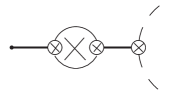
m. n.

Figure 7: Self energy insertion in external leg of a reduced graph. Minimal vertices are indicated by crosses: only the very left vertex can be non-minimal (case “n”).

The first one suits us, since relevant 2-leg graph contains only minimal vertices (m-type graphs). The second is uncomfortable since the very left vertex (that without cross) is non-minimal (n-type graphs).

To see that the latter insertion does not affect the $S$-matrix, we recall that the only part of two-point function contributing to the LSZ formula is the residue in the one-particle exchange pole, proportional to the wave function renormalization constant $Z$ (see e.g. Peskin Chaps. 7.1–7.2). Hadronic phenomenology says us that the highest spin we may need for external (stable) particle is $\frac{1}{2}$. So let us for definiteness work with nucleon propagator. The analysis below (we do not discuss mixing) can be easily adjusted for any spin, the scalar case is much simpler. The isospin structure is irrelevant for current discussion and, therefore, will be neglected.

For spin-$\frac{1}{2}$ particle the (parity conserving) amputated 1PI two-point function $\Sigma(p)$ (that contains all the contributions of both m and n types) can always be expressed via matrices $\hat{\bf 1}$ (the unit matrix) and ${\not{\!p}}$ as

$$\Sigma(p)=\sigma_{1}(\pi)\hat{\bf 1}+\sigma_{2}(\pi)({\not{\!p}}-m)\ ,\quad\pi\equiv p^{2}-m^{2}\ ,$$

so that the full propagator takes the form:

$$\raisebox{-12.91663pt}{\mbox{\includegraphics{sigma-small.eps}}}\equiv\frac{{\not{\!p}}+m}{\pi}+\frac{{\not{\!p}}+m}{\pi}\ \Sigma\ \frac{{\not{\!p}}+m}{\pi}+\ldots$$

$$=\frac{({\not{\!p}}+m)(1-{\sigma}_{2})+{\sigma}_{1}}{\pi(1-{\sigma}_{2})^{2}-2m{\sigma}_{1}(1-{\sigma}_{2})-{\sigma}^{2}_{1}}\;.$$ (41)

To keep the pole position in the physical mass $m$ we, therefore, need the prescription

$$\sigma_{1}(0)=0\ ,$$ (42)

while $\sigma_{2}$ does not affect the mass shift. Further, once the condition (42) holds, the full propagator near the pole is:

$$\left.\raisebox{-12.91663pt}{\mbox{\includegraphics{sigma-small.eps}}}\right|_{\scriptscriptstyle p_{0}\sim\sqrt{{\bf p}^{2}+m^{2}}}$$

$$=\frac{1}{1-\sigma_{2}(0)-2m\sigma^{\prime}_{1}(0)}\frac{{\not{\!p}}+m}{\pi}+\ldots\ ,$$ (43)

and the residue $Z_{f}=1$ is provided by the prescription

$$\sigma_{2}(0)+2m\sigma^{\prime}_{1}(0)=0\ .$$ (44)

First of all, let us show that the considered non-minimal insertions do not affect the pole position of the propagator (41). Indeed, for spin-$\frac{1}{2}$ case the only non-minimal tensor (matrix) structure is ${\not{\!p}}-m$. Hence, by its very definition, a non-minimal (w.r.t. external nucleon line) vertex brings extra factor $\pi$ or ${\not{\!p}}-m$, so the contribution to $\Sigma$ of the n-type graphs has the form:

$$\Sigma^{\rm\bf n}=\Sigma_{\rm s}\cdot\pi+\Sigma_{\rm t}\cdot({\not{\!p}}-m).$$

Besides, it is generally accepted that $\Sigma$ is regular near $p^{2}=m^{2}$ (nucleon is massive and stable); at any finite loop order it is justified by the very procedure of loop calculation. Then, decomposing the (matrices!) $\Sigma_{\rm s}$ and $\Sigma_{\rm t}$ through $\bf\hat{1}$ and ${\not{\!p}}\pm m$ one easily shows that the last expression can always be rewritten via some scalar (and regular in $\pi=0$) functions $\sigma_{s}$ and $\sigma_{t}$:

$$\Sigma^{\rm\bf n}=\pi\sigma_{\rm s}(\pi)\hat{\bf 1}+\sigma_{\rm t}(\pi)({\not{\!p}}-m)\ ,$$

so that the only contribution it may give to $\sigma_{1}$ is proportional to $\pi$ and, thereby, does not affect the condition (42). In fact, only the minimal piece of the on-shell contribution of m-type graphs (cf. Eq. (16)–(17)) can affect $\sigma_{1}(0)$, and it is set to zero by the RP (23) in Sec. VII (there is no imaginary part as the particle is stable). That is, to keep the correct pole position one just imposes the RP (23) on the graphs with only minimal (resultant) vertices and there is no need in the corresponding RP’s for graphs containing non-minimal vertices.

However, as seen from Eq. (43), the non-minimal vertices do affect the residue as they may contribute to $\sigma^{\prime}_{1}$ and $\sigma_{2}$. Here we shall follow another logics. Separating the contributions of m- and n-type graphs we can write the prescription (44) as

$$\sigma^{\rm\bf m}_{2}+2m(\sigma^{\rm\bf m}_{1})^{\prime}=-\left[\sigma^{\rm\bf n}_{2}+2m(\sigma^{\rm\bf n}_{1})^{\prime}\right]\quad{\rm at}\;p^{2}=m^{2}\ .$$ (45)

As usual, to fulfill it we must introduce counterterms. Working in effective theory at some fixed loop order, we can separately adjust counterterms for graphs of two different types, to be collectively denoted as $C^{\rm\bf m}_{{}_{Z}}$ and $C^{\rm\bf n}_{{}_{Z}}$, respectively. Now, according to the reduction theorem, the self-energy subgraphs with non-minimal vertices are not present inside the graph after the reduction, the only possibility is pictured in Fig. 7n. Hence, the adjusted $C^{\rm\bf n}_{{}_{Z}}$ can appear only on external legs replacing corresponding self-energy insertions and are never put inside the graph. In turn, any 2-leg insertion inside the graph is regulated by $C^{\rm\bf m}_{{}_{Z}}$ only and not affected by $C^{\rm\bf n}_{{}_{Z}}$. Simply speaking, the (non-minimal) RP’s for two-point graphs with non-minimal vertices decouple from the other set of RP’s. Only on external legs both $C^{\rm\bf m}_{{}_{Z}}$ and $C^{\rm\bf n}_{{}_{Z}}$ contribute. But, as it is seen from Eq. (45), whatever the m-type counterterms may be, their contribution on the left side can always be compensated by n-type counterterms on the right side so that the equality, and, thus, the condition (44) holds for external leg propagator. One can treat it as a manifestation of the well known fact that the wave function renormalization constant is a redundant parameter of a theory.

Practically it allows one to set $Z=1$ on the external legs automatically, having still a freedom in relevant (off-shell) counterterms for resultant (sub-)graphs. Then the LSZ formula says that we need to calculate only the resultant (amputated) graphs without self-energy insertions on external legs ($S$-matrix resultant graphs). In particular, graphs with non-minimal vertices can be discarded in the $S$-matrix calculations — that is exactly what we wanted to show.

Note also, that any additional mixing in external propagators due to non-minimal vertices can be excluded by the same arguments; though, as mentioned in Sec. VII, the problem of mixing which unavoidably arise whenever two-point function is discussed is beyond the scope of this article.

Unfortunately, the above reasoning does not give a hand to avoid non-minimal RP’s fixing the off-shell counterterms for graphs built of minimal vertices. In particular, corresponding 2-leg subgraphs will appear and may introduce off-shell subdivergencies (the on-shell behavior is, of course, regulated by RP (23)). Moreover, while in conventional renormalizable theories we are basically limited by first derivative of $\Sigma$, in effective theory other derivatives can also diverge. In forthcoming publication we will show that, accepting certain off-shell asymptotic conditions for the full sums of given type graphs (e.g. self-energy), one can avoid calculation of an infinite number of non-minimal counterterms and work directly with finite parts of those sums. In fact, the corresponding technique is already described in Secs. IV–VII.

References

- (1) A. Vereshagin and V. Vereshagin, Phys. Rev. D 69, 025002 (2004).
- (2) V. Vereshagin, Phys. Rev. D 55, 5349 (1997).
- (3) A. Vereshagin and V. Vereshagin, Phys. Rev. D 59, 016002 (1999).
- (4) A. Vereshagin, V. Vereshagin, and K. Semenov-Tian-Shansky, J. Math. Sci. 125, 144 (2005); translated from Zap. Nauchn. Sem. POMI 291, 78 (2002) (in Russian).
- (5) S. Weinberg, Physica A 96, 327 (1979).
- (6) S. Weinberg, The Quantum Theory of Fields, vols. 1–3 (Cambridge University Press, Cambridge, England, 2000).
- (7) A. Vereshagin and V. Vereshagin, Newsletter 15, 288 (1999); A. Vereshagin, Newsletter 16, 426 (2002).
- (8) K. Semenov-Tian-Shansky, A. Vereshagin, and V. Vereshagin, in AIP Conference Proceedings, Vol. 717, NY 2004: Tenth International Conference on Hadron Spectroscopy, Aschaffenburg, Germany, 2003, edited by E.Klempt, H.Koch, and H.Orth. See also talks given by the authors — to appear in Proceedings of international workshop “Hadron Structure and QCD: from LOW to HIGH energies”, St.Petersburg, Repino, Russia, 2004; Proceedings of the XVIIIth International Workshop “High Energy Physics and Quantum Field Theory”, St.Petersburg, Peterhof, Russia, 2004.
- (9) A. N. Vasil’ev, The Field Theoretic Renormalization Group in Critical Behavior Theory and Stochastic Dynamics (Chapman&Hall/CRC, NY, 2004; ISBN 0-415-31002-4).
- (10) J. C. Collins, Renormalization (Cambridge Univ. Press, Cambridge, 1984).
- (11) M. E. Peskin and D. V. Schroeder, Quantum Field Theory (Addison-Wesley, NY, 1997).
- (12) N. N. Bogoliubov and Y. A. Mitropolski, Asympthotic Methods in the Theory of Nonlinear Oscillations (Hindustan Publishing Corp., Delhi, Gordon and Breach, New York, 1961).
- (13) S. Coleman, Aspects of Symmetry (Cambridge University Press, Cambridge, 1985).
- (14) N. N. Bogoliubov, A. A. Logunov, and I. T. Todorov. Foundations of the axiomatic method in quantum field theory (Nauka, Moskow, 1969; in Russian).
- (15) S. Weinberg, Phys. Rev. 177, 2604 (1969).
- (16) C. Cronström and M. Noga, Nucl. Phys. B15, 61 (1970); A. Sudbery, Nucl. Phys. B20, 1 (1970); V. I. Ogievetskii, Sov. J. Nucl. Phys. 13, 105 (1971); S. R. Beane, Phys. Rev. D64, 116010 (2001).
- (17) W. Balser, From Divergent Power Series to Analytic Functions (Lecture notes in mathematics, Springer-Verlag, Berlin, 1994).
- (18) J. F. Chew, The analytic -matrix (W. A. Benjamin, Inc. New York, 1966).
- (19) A. Salam and J. Strathdee, Phys. Rev. D 2, 2869 (1970).
- (20) S. Weinberg, Phys. Rev. 133, B1318 (1964); ibid 134, B882 (1964); ibid 135, B1049 (1964); ibid 138, B988 (1965); ibid 181, 1893 (1969).
- (21) A. N. Vasiliev, Functional Methods in Quantum Field Theory and Statistical Physics (Gordon and Breach, Amsterdam, 1998).
- (22) S. Weinberg, Phys. Rev. 130, 2, 776; ibid 131, 1, 440; ibid 133, 1B, 232; M. Scadron and S. Weinberg, Phys. Rev. 133, 6B, 1589; M. Scadron, S. Weinberg and J. Wright, Phys. Rev. 135, 1B, 202.
- (23) M. Veltman, Physica 29, 186 (1963).
- (24) Particle Data Group, Review of Particle Physics, Phys. Letters B 592 (2004).
- (25) M. Harada, F. Sannino, and J. Schechter, Phys. Rev. D54, 1991 (1996); D. Black, A. Fariborz, F. Sannino, and J. Schechter, Phys. Rev. D58, 054012 (1998); ibid, D59, 074026 (1999); D. Black, A. Fariborz, S. Moussa, S. Nasri, and J. Schechter, Phys. Rev. D64, 014031 (2001).
- (26) S. Weinberg, in General Relativity — An Einstein Centenary Survey, ed. by S. W. Hawking and W. Israel (Cambridge University Press, Cambridge, England, 1979).
- (27) J. Gasser and H. Leutwyler, Ann. Phys. (N.Y.) 158, 142 (1984); Nucl. Phys. B250, 465 (1985).
- (28) D. J. Gross, Twenty five years of asymptotic freedom (arXiv:hep-th/9809060).
- (29) G. B. Arfken and H. J. Weber, Mathematical methods for physicists (Academic, New York, 1995); E. T. Whittaker and G. N. Watson, A course of modern analysis (Cambridge University Press, Cambridge, 1927).
- (30) G. Veneziano, Nuovo Cimento 57A, 190 (1968).
- (31) P. H. Frampton, Dual resonance models and superstrings (World Scientific, Singapore, 1986); M. B. Green, J. H. Schwarz, and E. Witten, Superstring theory (Cambridge University Press, Cambridge, 1987).