Casimir effect in a wormhole spacetime

Abstract

We consider the Casimir effect for quantized massive scalar field with non-conformal coupling $\xi$ in a spacetime of wormhole whose throat is rounded by a spherical shell. In the framework of zeta-regularization approach we calculate a zero point energy of scalar field. We found that depending on values of coupling $\xi$, a mass of field $m$, and/or the throat’s radius $a$ the Casimir force may be both attractive and repulsive, and even equals to zero.

I Introduction

The central problem of wormhole physics consists of the fact that wormholes are accompanied by unavoidable violations of the null energy condition, i.e., the matter threading the wormhole’s throat has to possess “exotic” properties. The classical matter does satisfy the usual energy conditions, hence wormholes cannot arise as solutions of classical relativity and matter. If they exist, they must belong to the realm of semiclassical or perhaps quantum gravity. In the absence of the complete theory of quantum gravity, the semiclassical approach begins to play the most important role for examining wormholes. Recently the self-consistent wormholes in the semiclassical gravity were studied numerically in Refs HocPopSus97 ; KhuSus02 ; Khu03 ; Gar05 . It was shown that the semiclassical Einstein equations provide an existence of wormholes supported by energy of vacuum fluctuations. However, it should be stressed that a natural size of semiclassical vacuum wormholes (say, a radius of wormhole’s throat $a$) should be of Planckian scales or less. This fact can be easily argued by simple dimensional considerations ForRom96 . In order to obtain semiclassical wormholes having scales larger than Planckian one has to consider either non-vacuum states of quantized fields (say, thermal states with a temperature $T>0$) or a vacuum polarization (the Casimir effect) which may happen due to some external boundaries (with a typical scale $R$) existing in a wormhole spacetime. In the both cases there appears an additional dimensional macroscopical parameter (say $R$) which may result in enlargement of wormhole’s size.

In this paper we will study the Casimir effect in a wormhole spacetime. For this aim we will consider a static spherically symmetric wormhole joining two different universes (asymptotically flat regions). We will also suppose that each universe contains a perfectly conducting spherical shell rounding the throat. These shells will dictate the Dirichlet boundary conditions for a physical field and, as the result, produce a vacuum polarization. Note that this problem is closely related to the known problem which was investigated by Boyer Boy68 who studied the Casimir effect of a perfectly conducting sphere in Minkowski spacetime (see also BorEliKirLes97 ). However, there is an essential difference which is expressed in different topologies of wormhole and Minkowski spacetimes. A semitransparent sphere as well as semitransparent boundary condition were investigated in Refs. BorVas99 ; Sca99 ; Sca00 ; BorVas04 ; GraJafKheQuaShrWei04 ; Mil04 . The consideration of the delta-like potential which models a semitransparent boundary condition in quantum field theory cause some problems and there is ambiguity in renormalization procedure (see the Refs. BorVas04 ; GraJafKheQuaShrWei04 ; Mil04 and references therein). Thermal corrections to the one-loop effective action on singular potential background was considered recently in Ref. MckNay05 .

We will adopt a simple geometrical model of wormhole spacetime: the short-throat flat-space wormhole which was suggested and exploited in Ref. KhuSus02 . The model represents two identical copies of Minkowski spacetime; from each copy a spherical region is excised, and then boundaries of those regions are to be identified. The spacetime of the model is everywhere flat except a throat, i.e., a two-dimensional singular spherical surface. We will assume that the wormhole’s throat is rounding by two perfectly conducting spherical shells (in each copy of Minkowski spacetime) and calculate the zero-point energy of a massive scalar field on this background. In the end of calculations the radius of one sphere will tend to infinity giving the Casimir energy for single sphere. For calculations we will use the zeta function regularization approach DowCri76 ; ZetaBook which was developed in Refs. Method ; BorEliKirLes97 ; KhuBor99 ; BezBezKhu01 ; BorMohMos01 . In framework of this approach, the ground state energy of scalar field $\phi$ is given by

$$E(s)=\frac{1}{2}\mu^{2s}\zeta_{\cal L}\left(s-\frac{1}{2}\right),$$ (1)

where

$$\zeta_{\cal L}(s)=\sum_{(n)}\left(\lambda_{(n)}^{2}+m^{2}\right)^{-s}$$

is the zeta function of the corresponding Laplace operator. The parameter $\mu$, having the dimension of mass, makes right the dimension of regularized energy. The $\lambda_{(n)}^{2}$ are eigenvalues of the three dimensional Laplace operator ${\cal L}=\triangle-\xi\mathcal{R}$

$$(\triangle-\xi\mathcal{R})\phi_{(n)}=\lambda_{(n)}^{2}\phi_{(n)},$$ (2)

where $\mathcal{R}$ is the curvature scalar (which is singular in framework of our model, see Eq. 6).

The expression 1 is divergent in the limit $s\to 0$ which we are interested in. For renormalization we subtract from 1 the divergent part of it

$$E^{\rm ren}=\lim_{s\to 0}\left(E(s)-E^{\rm div}(s)\right),$$ (3)

where

$$E^{\rm div}(s)=\lim_{m\to\infty}E(s).$$

By virtue of the heat kernel expansion of zeta function is the asymptotic expansion for large mass, the divergent part has the following form (in $3+1$ dimensions)

$$E^{\rm div}(s) = \frac{1}{2}\left(\frac{\mu}{m}\right)^{2s}\frac{1}{(4\pi)^{3/2}\Gamma(s-\frac{1}{2})}$$

$$\times \left\{B_{0}m^{4}\Gamma(s-2)+B_{1/2}m^{3}\Gamma(s-\frac{3}{2})+B_{1}m^{2}\Gamma(s-1)+B_{3/2}m\Gamma(s-\frac{1}{2})+B_{2}\Gamma(s)\right\},$$

where $B_{\alpha}$ are the heat kernel coefficients of operator ${\cal L}$. In the case of singular potential (singular scalar curvature) one has to use specific formulae from Refs. BorVas99 ; GilKirVas01 for calculation the heat kernel coefficients (see also a recent review Vas02 ).

Finally, the renormalized ground state energy 3 should obey the normalization condition

$$\lim_{m\to\infty}E^{\rm ren}=0.$$

For more details of approach see review BorMohMos01 .

The organization of the paper is the following. In Sec. II we describe a spacetime of wormhole in the short-throat flat-space approximation. In Sec. III we analyze the solution of equation of motion for massive scalar field and obtain close expression for zero point energy. In Sec. IV we discuss obtained results and make some speculations.

We use units $\hbar=c=G=1$. The signature of the spacetime, the sign of the Riemann and Ricci tensors, is the same as in the book by Hawking and Ellis HawEllBook .

II The geometry of the model

We will take a metric of static spherically symmetric wormhole in a simple form:

$$ds^{2}=-dt^{2}+d\rho^{2}+r^{2}(\rho)(d\theta^{2}+\sin^{2}\theta d\varphi^{2}),$$ (5)

where $\rho$ is a proper radial distance, $\rho\in(-\infty,\infty)$. The function $r(\rho)$ describes the profile of throat. In the paper we adopt the model suggested in the Ref. KhuSus02 which was called there as short-throat flat-space approximation. In framework of this model the shape function $r(\rho)$ is

$$r(\rho)=|\rho\,|+a,$$

with $a>0$. $r(\rho)$ is always positive and has the minimum at $\rho=0$: $r(0)=a$, where $a$ is a radius of throat. It is easy to see that in two regions ${\cal D}_{+}\!:\,\rho>0$ and ${\cal D}_{-}\!:\,\rho<0$ one can introduce new radial coordinates $r_{\pm}=\pm\rho+a$, respectively, and rewrite the metric 5 in the usual spherical coordinates:

$$ds^{2}=-dt^{2}+dr_{\pm}^{2}+r_{\pm}^{2}(d\theta^{2}+\sin^{2}\theta\,d\varphi^{2}),$$

This form of the metric explicitly indicates that the regions ${\cal D}_{+}$ and ${\cal D}_{-}$ are flat. However, note that such the change of coordinates $r_{\pm}=\pm\rho+a$ is not global, because it is ill defined at the throat $\rho=0$. Hence, as was expected, the spacetime is curved at the wormhole throat. To illustrate this we calculate the Ricci tensor in the metric 5:

$$\mathcal{R}^{\rho}_{\rho} = -\frac{2r^{\prime\prime}}{r}=-4\frac{\delta(\rho)}{a},$$

$$\mathcal{R}^{\theta}_{\theta}=\mathcal{R}^{\varphi}_{\varphi} = -\frac{-1+r^{\prime 2}+rr^{\prime\prime}}{r^{2}}=-2\frac{\delta(\rho)}{a},$$ (6)

$$\mathcal{R} = -\frac{2(-1+r^{\prime 2}+2rr^{\prime\prime})}{r^{2}}=-8\frac{\delta(\rho)}{a}.$$

The energy-momentum tensor corresponding to this metric has the diagonal form from which we observe that the source of this metric possesses the following energy density and pressure:

$$\varepsilon = -\frac{-1+r^{\prime 2}+2rr^{\prime\prime}}{8\pi r^{2}}=-\frac{\delta(\rho)}{2\pi a},\allowdisplaybreaks$$

$$p_{\rho} = \frac{-1+r^{\prime 2}}{8\pi r^{2}}=0,\allowdisplaybreaks$$

$$p_{\theta} = p_{\varphi}=\frac{r^{\prime\prime}}{8\pi r}=\frac{\delta(\rho)}{4\pi a}.$$

III Zero point energy

Let us now consider a scalar field $\phi$ in the spacetime with the metric 5. The equation for eigenvalues of operator ${\cal L}$ is

$$(\triangle-\xi{\cal R})\phi_{(n)}=\lambda_{(n)}^{2}\phi_{(n)},$$ (7)

where ${\cal R}$ is the scalar curvature, $\xi$ is an arbitrary coupling with ${\cal R}$ and $\triangle=g^{\alpha\beta}\nabla_{\alpha}\nabla_{\beta}$, $\alpha=1,2,3$. Due to the spherical symmetry of spacetime 5, a general solution to the equation 7 can be found in the following form:

$$\phi(\rho,\theta,\varphi)=u(\rho)Y_{ln}(\theta,\varphi),$$

where $Y_{ln}(\theta,\varphi)$ are spherical functions, $l=0,1,2,\dots$, $n=0,\pm 1,\pm 2,\dots,\pm l$, and a function $u(\rho)$ obeys the radial equation

$$u^{\prime\prime}+2\frac{r^{\prime}}{r}u^{\prime}+\left(\lambda^{2}-\frac{l(l+1)}{r^{2}}-\xi{\cal R}\right)u=0,$$ (8)

where a prime denotes the derivative with respect $\rho$, $\lambda=\sqrt{\omega^{2}-m^{2}}$ and scalar curvature ${\cal R}=-8\delta(\rho)/a$. For new function $w=ur$ this equation reads

$$w^{\prime\prime}+\left(\lambda^{2}-\frac{l(l+1)}{r^{2}}-\xi{\cal R}-\frac{r^{\prime\prime}}{r}\right)w=0,$$

and looks like the Schrödinger equation for massive particle with mass $M$ with total energy $E=\lambda^{2}/2M$ and potential energy

$$U=(\xi{\cal R}+\frac{r^{\prime\prime}}{r})/2M=\frac{1-4\xi}{aM}\delta(\rho).$$ (9)

Therefore, the $\xi>1/4$ corresponds to negative potential.

Unfortunately, in our case it is impossible to find in manifest form the spectrum of operator ${\cal L}$ given by Eq. 7. For this reason, we will use an approach developed in Refs. Method ; BorEliKirLes97 ; KhuBor99 ; BorMohMos01 ; BezBezKhu01 . This approach does not need an explicit form of spectrum. The spectrum of an operator is usually found from some boundary conditions which look like an equation $\Psi(\lambda)=0$ where function $\Psi$ consists of the solutions of Eq. 8 and depends additionally on other parameters of problem. It was shown in Refs. Method ; BorEliKirLes97 ; KhuBor99 ; BorMohMos01 ; BezBezKhu01 that the zero point energy may be represented in the following form:

$$E(s)=-\mu^{2s}\frac{\cos(\pi s)}{2\pi}\sum_{(n)}d_{n}\int_{m}^{\infty}dk(k^{2}-m^{2})^{1/2-s}\frac{\partial}{\partial k}\ln\Psi(ik),$$ (10)

with the function $\Psi$ taken on the imaginary axes. The sum is taken over all numbers of problem and $d_{n}$ is degenerate of state . This formula takes into account the possible boundary states, too. If they exist we have to include them additively at the beginning in the Eq. 1. But integration over interval $|k|<m$ (the possible boundary states exist in this domain) will cancel this contribution. For this reason the integration in the formula 10 is started from the energy $k=m$. Therefore, hereinafter we will consider the solution of the Eq. 8 for negative energy that is in imaginary axes $\lambda=ik$. The main problem is now reduced to finding the function $\Psi$. Thus, now we need no explicit form of spectrum of operator ${\cal L}$.

In the flat regions ${\cal D}_{\pm}$, where $r(\rho)=\pm\rho+a$, $r^{\prime}(\rho)=\pm 1$, ${\cal R}(\rho)=0$, and in imaginary axes the Eq.8 reads

$$u^{\prime\prime}+\frac{2}{\rho\pm a}u^{\prime}-\left(k^{2}+\frac{l(l+1)}{(\rho\pm a)^{2}}\right)u=0.$$ (11)

A general solution of this equation can be written as

$$u^{\pm}[k(a\pm\rho)]=A^{\pm}\sqrt{\frac{\pi}{2k(a\pm\rho)}}I_{\nu}[k(a\pm\rho)]+B^{\pm}\sqrt{\frac{\pi}{2k(a\pm\rho)}}K_{\nu}[k(a\pm\rho)],$$ (12)

where $I_{\nu},K_{\nu}$ are the Bessel functions of second kind, $\nu=l+1/2$, and $A^{\pm}$, $B^{\pm}$ are four arbitrary constants.

The solutions $u^{\pm}[k(\rho\pm a)]$ have been obtained in the flat regions ${\cal D}_{\pm}$ separately. To find a solution in the whole spacetime we must impose matching conditions for $u^{\pm}[k(\rho\pm a)]$ at the throat $\rho=0$. The first condition demands that the solution has to be continuous at $\rho=0$. This gives

$$u^{-}[ka]=u^{+}[ka].$$ (13a)

To obtain the second condition we integrate Eq.8 within the interval $$(-\epsilon,\epsilon) \epsilon\to 0$$ and then go to the limit . It gives the second condition

$$\left.-\frac{du^{-}[x]}{dx}\right|_{x=ka}=\left.\frac{du^{+}[x]}{dx}\right|_{x=ka}+\frac{8\xi}{ka}u^{+}[ka].$$ (13b)

Therefore, the general solution of Eq. 11 depends on two constants, only. Two other constants may be found from Eqs. 13a and 13b.

In addition to two matching conditions 13a and 13b we impose two boundary conditions. We round the wormhole throat by sphere of radius $a+R$ ($\rho=R$) in region ${\cal D}_{+}$, and by sphere of radius $a+R^{\prime}$ ($\rho=-R^{\prime}$) in region ${\cal D}_{-}$. Therefore the space of wormhole is divided by two spheres to three regions: the space of finite volume between spheres and two infinite volume spaces out of spheres. We suppose that the scalar field obeys the Dirichlet boundary condition on both of these spheres which means the perfect conductivity of spheres:

$$u^{-}[k(R^{\prime}+a)] = 0,$$ (13c)

$$u^{+}[k(R+a)] = 0.$$ (13d)

The four conditions 13 obtained represent a homogeneous system of linear algebraic equations for four coefficients $A^{\pm}$, $B^{\pm}$. As is known, such a system has a nontrivial solution if and only if the matrix of coefficients is degenerate. Hence we get

$$\left|\begin{array}[]{cccc}-I_{\nu}[ka]&-K_{\nu}[ka]&I_{\nu}[ka]&K_{\nu}[ka]\\ I^{\prime}_{\nu}[ka]+\frac{16\xi-1}{2ka}I_{\nu}[ka]&K^{\prime}_{\nu}[ka]+\frac{16\xi-1}{2ka}K_{\nu}[ka]&I^{\prime}_{\nu}[ka]-\frac{1}{2ka}I_{\nu}[ka]&K^{\prime}_{\nu}[ka]-\frac{1}{2ka}K_{\nu}[ka]\\ I_{\nu}[k(a+R)]&K_{\nu}[k(a+R)]&0&0\\ 0&0&I_{\nu}[k(a+R^{\prime})]&K_{\nu}[k(a+R^{\prime})]\end{array}\right|=0.$$ (14)

After some algebra the above formula can be reduced to the following relation for function $$\Psi$$ which we need for calculation of the energy 10:

$$\Psi_{in} = I_{\nu}[k(a+R^{\prime})]\left(\Psi^{*}\left[\left(\xi-\frac{1}{8}\right)K_{\nu}[ka]+\frac{ka}{4}K^{\prime}_{\nu}[ka]\right]-\frac{1}{8}K_{\nu}[k(a+R)]\right)$$

$$- K_{\nu}[k(a+R^{\prime})]\left(\Psi^{*}\left[\left(\xi-\frac{1}{8}\right)I_{\nu}[ka]+\frac{ka}{4}I^{\prime}_{\nu}[ka]\right]-\frac{1}{8}I_{\nu}[k(a+R)]\right)=0,$$

with

$$\Psi^{*}=I_{\nu}[k(a+R)]K_{\nu}[ka]-K_{\nu}[k(a+R)]I_{\nu}[ka].$$ (15)

In the case $$R^{\prime}=R \Psi_{in} \Psi_{in}=\Psi^{1}_{l}\Psi^{2}_{l}$$ above expression coincides with that obtained in Ref. KhuSus02 . In this case may be represented as follows: , where

$$\Psi^{1}_{l} = \Psi^{*}=I_{\nu}[k(a+R)]K_{\nu}[ka]-K_{\nu}[k(a+R)]I_{\nu}[ka],$$

$$\Psi^{2}_{l} = \left(\xi-\frac{1}{8}\right)\Psi^{*}+\frac{ka}{4}\left[I_{\nu}[k(a+R)]K^{\prime}_{\nu}[ka]-K_{\nu}[k(a+R)]I^{\prime}_{\nu}[ka]\right].$$

The solutions of Eq. 15 gives the spectrum of energies between the spheres $R$ and $R^{\prime}$. The spectra for regions out of these spheres can be found as follows:

$$\Psi_{out}^{1}=K_{\nu}[k(a+R)],$$ (15b)

$$\Psi_{out}^{2}=K_{\nu}[k(a+R^{\prime})].$$ (15c)

Indeed, let us consider the energy spectrum of field in space between two spheres with radii $R$ and $\widetilde{R}>R$ and Dirichlet boundary conditions on them. The solution is a linear combination of two modified Bessel functions

$$u_{R\widetilde{R}}=C_{1}I_{\nu}[k\rho]+C_{2}K_{\nu}[k\rho].$$

The Dirichlet boundary conditions give two equations

$$C_{1}I_{\nu}[k(a+R)]+C_{2}K_{\nu}[k(a+R)]=0,$$

$$C_{1}I_{\nu}[k(a+\widetilde{R})]+C_{2}K_{\nu}[k(a+\widetilde{R})]=0.$$

Using these equations we may represent the solution in the following form:

$$u_{R\widetilde{R}}=\frac{C_{1}}{K_{\nu}[k(a+R)]}\left\{I_{\nu}[k\rho]\frac{K_{\nu}[k(a+\widetilde{R})]}{I_{\nu}[k(a+\widetilde{R})]}-K_{\nu}[k\rho]\right\}.$$

Let us now assume that $\widetilde{R}\to\infty$. In this limit the solution takes the following form:

$$u_{R\infty}=CK_{\nu}[k\rho].$$

The Dirichlet boundary condition for this solution on the sphere of radius $R$ gives the equation 15b. As expected this condition coincides with expression for space out of sphere of radius $a+R$ in Minkowski spacetime BorEliKirLes97 . It is obviously because the spacetime out of sphere (in general out of throat) is exactly Minkowski spacetime.

Therefore the regularized total energy 10 reads

$$E(s)=-\mu^{2s}\frac{\cos(\pi s)}{\pi}\sum_{l=0}^{\infty}\nu\int_{m}^{\infty}dk(k^{2}-m^{2})^{1/2-s}\frac{\partial}{\partial k}\left[\ln\Psi_{in}+\ln\Psi_{out}^{1}+\ln\Psi_{out}^{2}\right].$$ (16)

Regrouping terms we can rewrite the above formula in the form having clear physical sense of each term:

$$E(s)=\triangle E(s)+E_{R}^{M}(s)+E_{R^{\prime}}^{M}(s),$$ (17)

where

$$E_{R}^{M}(s) = -\mu^{2s}\frac{\cos(\pi s)}{\pi}\sum_{l=0}^{\infty}\nu\int_{m}^{\infty}dk(k^{2}-m^{2})^{1/2-s}\frac{\partial}{\partial k}\ln I_{\nu}[k(a+R)]K_{\nu}[k(a+R)],$$ (18)

$$E_{R^{\prime}}^{M}(s) = -\mu^{2s}\frac{\cos(\pi s)}{\pi}\sum_{l=0}^{\infty}\nu\int_{m}^{\infty}dk(k^{2}-m^{2})^{1/2-s}\frac{\partial}{\partial k}\ln I_{\nu}[k(a+R^{\prime})]K_{\nu}[k(a+R^{\prime})],$$ (19)

$$\triangle E(s) = -\mu^{2s}\frac{\cos(\pi s)}{\pi}\sum_{l=0}^{\infty}\nu\int_{m}^{\infty}dk(k^{2}-m^{2})^{1/2-s}\frac{\partial}{\partial k}\ln\Psi$$ (20)

and

$$\Psi=\frac{\Psi_{in}}{I_{\nu}[k(a+R^{\prime})]I_{\nu}[k(a+R)]}$$

The term $E_{R}^{M}(s)$ in the formula 17 is nothing but a zero point energy of sphere of radius $a+R$ in Minkowski spacetime with Dirichret boundary condition on the sphere BorEliKirLes97 ; note that the term $E_{R^{\prime}}^{M}(s)$ has an analogous sense.

Now we are ready to calculate the Casimir energy for two spherical boundaries by using expression 16 and Eq. 3. Then let us consider the Boyer’s problem. We consider ”gedanken experiment”: we take a single conducting sphere and measure the Casimir force in this situation. For this reason we have to take a limit $R^{\prime}\to\infty$. In this case the energy 19 tends to zero, and so the term $\triangle E(s)$ in Eq. 20 represents the difference between Casimir energies of a sphere rounding the wormhole and a sphere of the same radius in Minkowski spacetime without wormhole. In the limit $R^{\prime}\to\infty$ we find

$$\Psi=\left(K_{\nu}[ka]-I_{\nu}[ka]\frac{K_{\nu}[k(a+R)]}{I_{\nu}[k(a+R)]}\right)\left(\left(\xi-\frac{1}{8}\right)K_{\nu}[ka]+\frac{ka}{4}K^{\prime}_{\nu}[ka]\right)-\frac{1}{8}\frac{K_{\nu}[k(a+R)]}{I_{\nu}[k(a+R)]}$$ (21)

If one turns $R\to\infty$ then the energy $E^{M}_{R}$ tends to zero and so

$$\Psi\to K_{\nu}[ka]\left(\left(\xi-\frac{1}{8}\right)K_{\nu}[ka]+\frac{ka}{4}K^{\prime}_{\nu}[ka]\right).$$ (22)

This expression coincides exactly with that obtained in Ref. KhuSus02 and describes the zero point energy for whole wormhole spacetime without any additional spherical shells.

A comment is in order. As already noted the positive $\xi$ corresponds to attractive potential and therefore the boundary states may appear. The appearance of boundary states with delta-like potential has been observed in Ref. MamTru82 . Thus, we have to take into account the boundary states at the beginning. Nevertheless, the final formula 16 contains these boundary states, as it was noted in Ref. Method . But it is necessary to note, that in this paper we will consider $\xi<1/4$. Indeed, let us consider for example $l=0$. In this case

$$\Psi=\frac{\pi}{8}e^{-ka}\cosh(k(a+R))\left\{\cosh(kR)+\left[2\frac{1-4\xi}{ka}+1\right]\sinh(kR)\right\}.$$

For $\xi>1/4$ this expression may be equal to zero for some value of $k>m$, $R$ and $a$ and integral 16 will be divergent. As noted in Ref. MamTru82 in this case we can not use the present theory. The same boundary for $\xi$ was noted in Ref. KhuSus02 . This statement is easy to see from expression for potential energy given by Eq. 9. For $\xi>1/4$ the energy is negative and the boundary states may appear.

The general strategy of the subsequent calculations is following (for more details see Refs. Method ; BorEliKirLes97 ; KhuBor99 ; BorMohMos01 ; BezBezKhu01 ). To single out in manifest form the divergent part of regularized energy we subtract from and add to integrand in Eq. 16 its uniform expansion over $1/\nu$. It is obviously that it is enough to subtract expansion up to $1/\nu^{2}$, the next term will give the converge series. We may set $s=0$ in the part from which we had subtracted the uniform expansion because it is now finite (see Eq. 26). The divergent singled out part will contain the standard divergent terms given by Eq. I and some finite terms which we calculate in manifest form (all terms except $A$ in 23).

The uniform asymptotic expansions both 21 and 22 are the same for $R\not=0$. Indeed, in this case the ratios

$$\frac{I_{\nu}[ka]}{K_{\nu}[ka]}\frac{K_{\nu}[k(a+R)]}{I_{\nu}[k(a+R)]} \approx e^{-2\nu\ln(1+\frac{R}{a})},$$

$$\frac{1}{K^{2}_{\nu}[ka]}\frac{K_{\nu}[k(a+R)]}{I_{\nu}[k(a+R)]} \approx 2\nu e^{-2\nu\ln(1+\frac{R}{a})}$$

are exponentially small and we may neglect them. The well-known uniform expansions of Bessel functions AbrSte were used in these expressions. For this reason we may disregard this fraction in Eq. 21 and arrive to Eq. 22. This is a key observation for next calculations. Due to this observation the divergent part which we have to subtract for renormalization from 20 has been already calculated in Ref. KhuSus02 . By using the results of this paper we may write out the expression for renormalized zero point energy:

$$\triangle E = -\frac{1}{32\pi^{2}a}\left(b\ln\beta^{2}+\Omega\right),$$ (23)

$$\Omega = A+\sum_{k=-1}^{3}\omega_{k}(\beta),$$ (24)

$$b = \frac{1}{2}b_{0}\beta^{4}-b_{1}\beta^{2}+b_{2},$$ (25)

where

$$A = 32\pi\sum_{l=0}^{\infty}\nu^{2}\int_{\beta/\nu}^{\infty}dy\sqrt{y^{2}-\frac{\beta^{2}}{\nu^{2}}}\frac{\partial}{\partial y}\left(\ln\Psi+2\nu\eta(y)+\frac{1}{\nu}N_{1}-\frac{1}{\nu^{2}}N_{2}+\frac{1}{\nu^{3}}N_{3}\right),$$ (26)

$$\Psi = \left(K_{\nu}[\nu y]-I_{\nu}[\nu y]\frac{K_{\nu}[\nu y(1+x)]}{I_{\nu}[\nu y(1+x)]}\right)\left(\left(\xi-\frac{1}{8}\right)K_{\nu}[\nu y]+\frac{\nu y}{4}K^{\prime}_{\nu}[\nu y]\right)-\frac{1}{8}\frac{K_{\nu}[\nu y(1+x)]}{I_{\nu}[\nu y(1+x)]},$$ (27)

$b_{k}$ are the heat kernel coefficients, $\beta=ma$ is a dimensionless parameter of mass, and $x=R/a$ is a dimensionless parameter of sphere’s radius. The explicit form of heat kernel coefficients $b_{k}$, and also expressions for $\omega_{k},\ N_{k},\ \eta$ are given in the Ref. KhuSus02 . Note that they do not depend on the radius of sphere $R$. The only dependence on $R$ is contained in the coefficient $A$ which has to be calculated numerically. The expression for contribution of the sphere in Minkowski spacetime 18 may be found in Ref. BorEliKirLes97 . We only have to make a change $R\to a+R$.

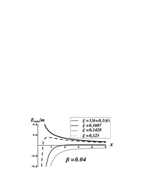
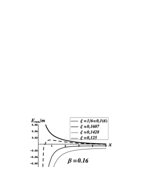
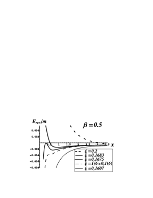
Figure 1: The plots of renormalized zero-point energy $E_{ren}/m$ as a function of $x=R/a$ for $\beta=0.04,0.16,0.5$ and for various values of $\xi$ and fixed mass $m$. We observe that increasing $\xi$ leads to appearance maximum and/or minimum. For subsequent increasing $\xi$ the curve will turn over and extremum disappears. If the radius of spherical shell exceeds ten radius of throat the zero-point energy takes on a value which equals to zero-point energy in whole wormhole spacetime.

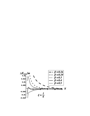
Figure 2: The plot of $\triangle E_{ren}/m$ as a function of $x=R/a$ for $\xi=\frac{1}{6}$ and for various values of $\beta$ and fixed mass $m$. We observe the dynamics of deformation of energy due to changing the parameter $\beta=ma$ for fixed $\xi$.

IV Discussion and conclusion

In this section we will discuss results of numerical calculations of zero-point energy given by formula 23. The renormalized zero-point energy is represented in figures 1, 2 as a function of $x=R/a$ (the position of sphere rounding the wormhole) for various values of $\beta=ma$ and $\xi$. (Note that the value $x=R/a$ characterizes the position of sphere rounding the wormhole; $x=0$ corresponds to sphere’s radius equals to throat’s radius.) In Fig. 1 we only show the full energy $E$. Note that the $\triangle E$ differs just slightly from the full energy $E$. For the same reason we reproduce in Fig. 2 the $\triangle E$, only.

Characterizing the result of calculations we should first of all stress that the value of zero point energy $E_{ren}$ in the limit $R\to\infty$ tends to some constant value obtained in Ref. KhuSus02 for the case of wormhole spacetime without any spherical shells. In the limit $R\to 0$ (i.e., when the sphere radius $a+R$ tends to the throat’s radius $a$) the zero-point energy $E_{ren}$ is infinitely decreasing for all $\beta$ and $\xi$. This means that the Casimir force acting on the spherical shell and corresponding to the Casimir zero point energy $E_{ren}$ is “attractive”, i.e., it is directed inward to the wormhole’s throat, for sufficiently small values of $R$. In the interval $0<R/a<\infty$ there are three qualitatively different cases of behavior of $E_{ren}$ depending on values of $\beta$ and $\xi$. Namely, (i) the zero point energy $E_{ren}$ is monotonically increasing in the whole interval $0<R/a<\infty$. There are neither maxima no minima in this case. Hence the Casimir force is attractive for all positions of the spherical shell. (ii) $E_{ren}$ is first increasing and then decreasing. A graph of the zero point energy has the form of barrier with some maximal value of $E_{ren}$ at $R_{1}/a$. The Casimir force is attractive for the sphere’s radius $R<R_{1}$ and repulsive for $R>R_{1}$. The value $R=R_{1}$ corresponds to the point of unstable equilibrium. (iii) The zero point energy $E_{ren}$ is increasing for $R/a<R_{1}/a$, decreasing for $R_{1}/a<R/a<R_{2}/a$ and then finally increasing for $R/a>R_{2}/a$, so that a graph of $E_{ren}$ has a maximum and minimum. In this case the Casimir force is directed outward provided the sphere’s radius $R_{1}<R<R_{2}$, and inward provided $R<R_{1}$ or $R>R_{2}$. Now the value $R=R_{2}$ corresponds to the point of stable equilibrium, since the zero point energy $E_{ren}$ has here a local minimum.

It is worth noting that the Casimir force is attractive in the whole interval $0<R/a<\infty$ for sufficiently small values of $\xi$ and/or large values of $\beta$. Otherwise, it can be both attractive and repulsive depending on a radius of sphere rounding the wormhole’s throat. The similar situation appears for delta-like potential on the spherical or on the cylindrical boundaries Sca99 ; Sca00 . The repulsive Casimir force was also observed in Ref. HerSam05 for scalar field living in the Einstein Static Universe.

The considered model let us speculate in spirit of Casimir idea who suggested a model of electron as a charged spherical shell Cas56 . Casimir assumed that such a configuration should be stable due to equilibrium between the repulsive Coulomb force and the attractive Casimir force. However, as is known, this idea does not work in Minkowski spacetime since the Casimir force for sphere turns out to be repulsive Boy68 . Now one can revive the Casimir’s idea by considering a spherical shell rounding the wormhole. In this paper we have shown that the Casimir force now can be both attractive and repulsive. Moreover, there exists stable configurations for which the Casimir force equals to zero; the radius of spherical shell in this case depends on the throat’s radius $a$ as well as the field’s mass $m$ and coupling constant $\xi$. Thus, one may try to realize the Casimir’s idea taking a sphere rounding a wormhole. Of course, our consideration was based on the very simple model of wormhole spacetime. However, we believe that main features of above consideration remain the same for more realistic models.

- (1) M. Abramowitz and I.A. Stegun, Handbook of Mathematical Functions, (US National Bureau of Standards, Washington, 1964)
- (2) E.R. Bezerra de Mello, V.B. Bezerra and N.R. Khusnutdinov, J. Math. Phys. 42, 562 (2001)
- (3) M. Bordag, J. Phys. A 28, 755 (1995); M. Bordag and K. Kirsten, Phys. Rev. D 53, 5753 (1996); M. Bordag, K. Kirsten, and E. Elizalde, J. Math. Phys. 37, 895 (1996); M. Bordag, K. Kirsten, and D. Vassilevich, Phys. Rev. D 59, 085011 (1999).
- (4) M. Bordag, E. Elizalde, K. Kirsten, and S. Leseduarte, Phys. Rev. D 56, 4896 (1997)
- (5) M. Bordag and D.V. Vassilevich, J. Phys. A 32, 8247 (1999)
- (6) M. Bordag M. U. Mohideen, V.M. Mostepanenko, Phys. Rep. 353, 1 (2001)
- (7) M. Bordag and D.V. Vassilevich, Phys. Rev. D 70, 045003 (2004)
- (8) T.H. Boyer, Phys. Rev. 174, 1764 (1968)
- (9) H.B.G. Casimir, Physica 19, 846 (1956)
- (10) J. S. Dowker and R. Critchley, Phys. Rev. D 13, 3224 (1976); W. Hawking, Commun. Math. Phys. 55, 133 (1977); S. K. Blau, M. Visser, and A. Wipf, Nucl. Phys. B 310, 163 (1988)
- (11) E. Elizalde, S. D. Odintsov, A. Romeo, A. A. Bytsenko, and S. Zerbini, Zeta Regularization Techniques with Applications, (World Scientific, Singapore, 1994)
- (12) L.H. Ford, T. A. Roman, Phys. Rev. D 53, 5496 (1996); K.K. Nandi, Y.Z. Zhang and Kumar K.B. Vijaya Phys. Rev. D 70, 064018 (2004)
- (13) R. Garattini, Class. Quant. Grav., 22 1105 (2005)
- (14) P.B. Gilkey, K. Kirsten, and D.V. Vassilevich, Nucl. Phys. B601, 125 (2001)
- (15) N. Graham, R.L. Jaffe, V. Khemani, M. Quandt, O. Schroeder, and H. Weigel, Nucl. Phys. B677, 379 (2004)
- (16) S.W. Hawking and G.F.R. Ellis, The Large Scale Structure of spacetime, (Cambridge University Press, Cambridge, London, 1973)
- (17) C.A.R. Herdeiro, M. Sampaio, hep-th/0510052
- (18) D. Hochberg, A. Popov, S. V. Sushkov, Phys. Rev. Lett. 78, 2050 (1997)
- (19) N.R. Khusnutdinov and M. Bordag, Phys. Rev. D 59, 064017 (1999).
- (20) N.R. Khusnutdinov and S.V. Sushkov, Phys. Rev. D 65, 084028 (2002)
- (21) S.G. Mamaev and N.N. Trunov, Yadernaya Fiz. 35, 1049 (1982) [in Russian]
- (22) J.J. Mckenzie-Smith, and W. Naylor, Phys. Lett. B610, 159 (2005)
- (23) N.R. Khusnutdinov, Phys. Rev. D 67, 124020 (2003); Theor. Math. Phys. 138(2), 250 (2004)
- (24) K. Milton, J. Phys. A: Math. Gen. 37, 6391 (2004)
- (25) M. Scandurra, J. Phys. A 32, 5679 (1999)
- (26) M. Scandurra, J. Phys. A 33, 5707 (2000)
- (27) D. Vassilevich, Phys. Rep. 388, 279 (2003)