Polyakov’s String: Twenty Five Years After

Table of contents

• Preface page 01

• Valery Pokrovsky
  Hydden Sasha Polyakov’s life
  in Statistical and Condensed Matter Physics page 02

• Alexander Belavin and Alexei Zamolodchikov
  Moduli Integrals, Ground Ring and Four-Point Function in
  Minimal Liouville Gravity page 16

• Yukitaka Ishimoto and Alexei Zamolodchikov
  Massive Majorana Fermion Coupled to 2D Gravity and Random
  Lattice Ising Model page 47

Предисловие

В Июне 2005 года в Черноголовке состоялась Международная Конференция, посвященная ‘‘Струне Полякова’’. По идее оргкомитета, кроме 25-летней годовщины появления Струны Полякова [1], эта конференция была приурочена также к 35-летию открытия Конформной Инвариантности [2], 30-летию Монополя [3] и Инстантонов [4] и, наконец, 20-летию Конформной Теории Поля [5]. И, по редкому совпадению, к круглой годовщине со дня рождения самого Саши, перечисленный выше список достижений которого далеко не исчерпывает его вклада в Теоретическую Физику 20-го века.

И хотя нам не удалось собрать достаточно представительную конференцию (соответственно, доклады, приведенные в настоящем Сборнике, отражают развитие идей Полякова в высшей степени фрагментарно), нам представляется важным, что она произошла именно в Черноголовке, месте, где много лет, в Институте Теоретической Физики Л.Д.Ландау, работал Александр Поляков.

The International Workshop dedicated to an anniversary of the Polyakov’s String (of course today there is no need to remind the meaning and the role of this theory) was held in Chernogolovka in June 2005. Apart from the 25-th anniversary of the first appearance of the Polyakov’s String theory [1], this conference, to our mind, might be also thought of as a 35 years from the discovery of the Conformal Invariance [2], 30 years of the Monopole [3] and the Instantons [4] and, finally, as the 20-th anniversary of the CFT [5]. A case of mysterious coincidence, this year is also a jubilee of Sasha himself, whose contribution to the Theoretical Physics of 20-th century is far from being exhausted by the achievements listed above.

Although we haven’t managed to bring together a really representative conference (consequently, the talks delivered give only a fragmentary and incomplete picture of the developments of Sasha’s ideas), we find it significant, that it took place Chernogolovka, where during many years Alexander Polyakov worked in the Landau Institute of Theoretical Physics.

Оргкомитет

1
Introduction

History of Science (is it a Science itself?) shows that the greatest field and elementary particle theorists felt an insistent necessity to make something in a more earthly subjects. I do not speak about such universal giants as Bethe, Fermi and Landau, for whom there was no separation between different parts of physics. But their younger and more specialized contemporaries also time to time did seminal works in statistical or condensed matter physics. An example is the brilliant work by Feynman on vortices in a superfluid and his unpublished work on vortices in 2D XY-magnet repeated independently in a famous articles by Berezinskii and by Kosterlitz and Thouless. A fundamental contribution into Statistical Physics was done by Gell-Mann and Bruckner in their work on the virial expansion of weakly interacting Fermi-gas. Lee and Yang theorem on the distribution of nodes of the partition function became one of the cornerstones of the phase transition theory. C.N. Yang probably has the longest list of fundamental works in statistical physics, which includes, besides of the mentioned work, the derivation of the Onsager formula for the magnetization of the Ising magnet (1952, theory of 1D interacting Fermi-gas (together with C.P. Yang, 1965), virial expansion for weakly interacting Bose gas (together with T.D. Lee) and recent works on Bose-Einstein condensation.

The response to these works was always very vivid and eager. Apart of the undoubted merits of the works it can be explained by a simple psychological effect: it is flattering to occur in touch with the deepest minds of humanity.

Even in this company, Sasha Polyakov’s works are probably most popular in the earthly physics. Despite Sasha’s carelessness about experimental consequences of his theories and real figures his works occurred very close to real experiments, most of them in Condensed Matter Physics. They also played very important role for development of Statistical Physics and Condensed Matter Theory. Below I give a brief review of the life of Sasha’s ideas, sometimes unexpected, sometimes rediscovered in other terms. Most of them were conceived as field-theoretical works with no intended application to Condensed Matter Physics.

2 Phase Transitions and Critical Phenomena

No surprise that the Quantum Field Theory can be applied in Statistical Physics. As it was demonstrated by many people the two subjects are almost identical: statistics is a Euclidian field theory. In his book [1] Sasha suggested that this analogy is more than a formal trick, that it may stem from a deep, not yet understood physics associated with the nature of time. Leaving this philosophical question for future, we turn to the Polyakov’s works.

2.1 Bootstrap theory of Phase Transitions

The first Sasha’s intervention into the Phase Transition theory was his article of 1968 [2], just at the end of his ”Aspirantura”. In this work he moved opposite to the standard approach replacing the Euclidian field theory by pseudoeuclidean one. The purpose of this trick was to employ the unitarity condition and avoid a rather doubtful subtraction procedure, which Patashinskii and I applied in our earlier work on the same topic published in 1964 [3]. At that moment we already understood something is wrong in our work, but we did not know what. In Sasha’s work the wrong point was explicitly found and reformulated correctly. It was so exciting that, when Sasha by my request visited me in a hospital where I stayed already for a while, I immediately have felt myself recovered, an unrecorded case of miraculous healing. To my surprise and enjoyment it occurred that a large part of our work (scaling) was correct.

Although the bootstrap equations in principle determined critical exponents, they were too complicated to allow numerical calculations, at least at that time. I believe that now it would be possible by employing a modification of the bootstrap equations proposed by Sasha Migdal [4] (independently and with very small difference in time) and three-point correlators derived by AP in 1970 (see subsection Conformal invariance). Unfortunately, the train has departed in 1972 bringing the Nobel Prize with it.

2.2 Algebra of fluctuating fields

In 1969 Sasha introduced a new concept: algebra of fluctuating fields [6] (independently the same discovery was made by Leo Kadanoff [7]). He suggested that any fluctuating field in a vicinity of the phase transition point can be expanded in a basis (generally infinite) of basic fields $A_{n}(\mathbf{x})$ characterized by their scaling dimensionality $\Delta_{n}$. The product of two such fields taken at close points can be also expanded in the same basis. The three-point coefficients of this expansion describe the triple interaction between the fields and completely determine the algebra. This idea not only simplified enormously the structure of the phase transition theory, but also gave it a new dimension. Till 1969 only the order parameter and the entropy (energy) density were considered as basic fluctuating fields. The algebra revealed a multitude of other fields.

2.3 Conformal invariance

In 1970 Sasha conjectured that symmetry of the effective field theory at phase transition point is much more extensive than the global scaling group. In the spirit of the gauge field theory by Yang and Mills, the scaling symmetry must be local with the scale factor varying in space retaining local isotropy. The transformations performing this job form the conformal group. Some its implications were studied earlier in the quantum field theory, but Sasha was the first to derive its consequences for correlation functions. For two-point correlators in any dimension he found the orthogonality condition $\langle A(\mathbf{x})B(\mathbf{x}^{\prime})\rangle=0$ if $\Delta_{A}\neq\Delta_{B}$. Moreover, he showed that the conformal invariance completely determines the 3-point correlator and obtained a beautiful formula for it:

$$\langle A_{1}(\mathbf{x}_{1})A_{2}(\mathbf{x}_{2})A_{3}(\mathbf{x}_{3})\rangle=\frac{\Gamma_{123}}{|\mathbf{x}_{1}-\mathbf{x}_{2}|^{\Delta_{1}+\Delta_{2}-\Delta_{3}}|\mathbf{x}_{2}-\mathbf{x}_{3}|^{\Delta_{2}+\Delta_{3}-\Delta_{1}}|\mathbf{x}_{3}-\mathbf{x}_{1}|^{\Delta_{3}+\Delta_{1}-\Delta_{2}}}$$ (2.1)

To my knowledge no attempts was made to measure 3-point correlators. All scattering methods measure 2-point correlators. A reasonable way to find 3-point correlators would be to measure the dependence of a 2-point correlator on weak oscillatory perturbations, for example, sound. The experiment looks difficult since the temperature and pressure in critical measurements must be fixed with very high precision. The perturbation should be very weak to retain such a high precision. Nevertheless, such an experiment seems feasible.

In the same work Sasha noted that the conformal group in 2 dimensions is very reach: it is well-known group of conformal transformation of a complex variable $z=x+iy$ provided with any analytic function $w(z)$. Sasha anticipated that irreducible representations of this group completely determine all possible types of critical behavior (universality classes) in 2 dimensions. This program was realized only 13 years later in a famous work by Belavin, Polyakov and Zamolodchikov [8]. Enormous number of journal articles and many books developed and reviewed this theory. I will not make any attempt to describe it in this brief review. I only note that indeed all known types of critical behavior including exactly solved Ising model, 8-vertex and Ashkin-Teller models, Potts model, their multicritical points and an infinite class of model by Andrews and Baxter, Heisenberg model etc. took their place as special representations of the Conformal Group.

2.4 Multi-component vector model and real magnets

In 1971-72 Vadim Berezinskii had published two seminal articles on 2-dimensional XY-model with global symmetry group SO(2) or U(1) [9]. He discovered the algebraic order in this system and its destruction by vortices. In the first of these works he stated that 3-component and more generally n-component vector model with the non-abelian symmetry group SO(n) also has algebraic order. In 1975 Sasha revised this problem [10] and has found that strong interaction generated by the non-abelian group and its topology completely changes the physical properties of the vector fields. In particular, he found that there is no phase transition in the model for $n\geq 3$ and the ordering field acquires mass at large distances at any temperature.

The n-vector model is a model of a classical vector field with the Hamiltonian

$$H=\frac{J}{2}\int(\nabla\mathbf{n(x)})^{2}d^{2}x,$$ (2.2)

where $\mathbf{n(x)}$ is an n-component vector of unit length. Employing a clever renormalization procedure conserving the length of the vector, Sasha found a remarkable result for the dependence of the order parameter $M=|\langle\mathbf{n}\rangle|$ on scale $L$:

$$M=\left(1-\frac{(n-2)T}{4\pi J}\ln\frac{L}{a}\right)^{\frac{n-1}{2(n-2}}$$ (2.3)

This result known as Polyakov’s renormalization has some limitations. Namely, the ratio $T/4\pi J$ must be small and the value $M$ must be much larger than $T/4\pi J$, though it can be much smaller than 1. At the distances $L\gg R_{C}=a\exp(4\pi J/T)$ the expected behavior of $M(L)$ is $M=\exp(-L/R_{c})$. The renormalization group does not work at such long distances. The conjecture about exponential decay of correlations was confirmed later by exact calculations (Polyakov and Wiegmann [11]). Physically the strong renormalization stems from strong fluctuations generated by Goldstone modes (spin waves). At $n=2$ the equation (2.3) reproduces the Berezinskii’s algebraic order. At $n=3$ corresponding to isotropic (Heisenberg) magnet the equation (2.3) is strongly simplified:

$$M=1-\frac{T}{4\pi J}\ln\frac{L}{a}$$ (2.4)

In real magnets the isotropy is slightly violated by spin-orbit and dipolar interactions or by an external magnetic field. This violation fixes the length scale $L_{A}=\sqrt{J/A}$, where $A$ is the amplitude of the symmetry-violating field, for example a coefficient in the additional term $An_{z}^{2}$ in the Hamiltonian. If the length $L_{A}$ is much less than the correlation length $R_{c}$, the magnetization is given by equation (2.4) with $L=L_{A}$. The linear dependence of magnetization on temperature in weakly anisotropic magnets is a firmly established experimental fact. It was found in many materials by many authors. In Fig. 1 we demonstrate the experimental dependence $M(T)$ for an ultrathin iron film on the surface Ag(111) found by Z. Qiu et al. [12] by the measurement of the surface magneto-optic Kerr effect (SMOKE). The linear dependence takes place at $T/T_{c}$ from 0 to 0.95. Close to the Curie point they observed the critical behavior $M\propto(T_{c}-T)^{1/8}$.

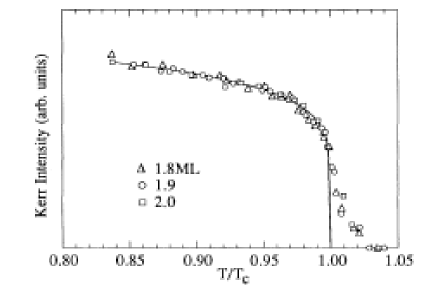
Figure 1: Magnetization vs. temperature

2.5 Quantum Phase Transitions

In his book [1] published in 1987 Sasha considered probably the first model displaying the Quantum Phase Transition in two space dimensions. It was the lattice of quantum rotators. In this model plane quantum rotators are placed at sites $\mathbf{a}$ of a regular lattice. Each rotator is characterized by its rotation angle $\varphi_{\mathbf{a}}$ or alternatively by its angular momentum $\hat{n}_{\mathbf{a}}$ with the standard commutation relation $\left[\hat{n}_{\mathbf{a}},\varphi_{\mathbf{a}^{\prime}}\right]=-i\delta_{\mathbf{a,a}^{\prime}}$. The eigenvalues of $\hat{n}_{\mathbf{a}}$ are integers. The Hamiltonian of the model reads:

$$H=\frac{K}{2}{\displaystyle\sum\limits_{\mathbf{a}}}\hat{n}_{\mathbf{a}}^{2}-J{\displaystyle\sum\limits_{(\mathbf{a,a}^{\prime})}}\cos\left(\varphi_{\mathbf{a}}-\varphi_{\mathbf{a}^{\prime}}\right)$$ (2.5)

The summation in the lust sum of equation (2.5) proceeds over the pairs of nearest neighbors. The competition between ”kinetic” and ”potential” energy results in a phase transition at zero temperature from the ”ordered” state with $\left\langle\cos\varphi_{\mathbf{a}}\right\rangle\neq 0$ and indefinite $\hat{n}_{\mathbf{a}}$ at $J>K$ to the ”disordered state with all $\hat{n}_{\mathbf{a}}=0$ and $\left\langle\cos\varphi_{\mathbf{a}}\right\rangle=0$ at $J<K$. The tuning of the ratio $J/K$ could be produced by pressure. The spin version of the model can be formulated for spins $S\geq 1$. This is the Heisenberg model with the strong anisotropy term $KS_{z}^{2}$.

The problem of quantum phase transitions became rather popular last 15 years in connection with High-T_c superconductors, magnetic chains, metal-insulator transitions etc. The detailed description of the state of art is given in the book by Sachdev [13].

3 Topological Excitations

In the beginning of 1970-th after the Berezinskii’s work on vortices in XY-magnets [9], Sasha has asked me what kind of objects are vortices. Are they quasiparticles? I answered that in 3 dimensions the vortex rings are indeed quasiparticles with the dispersion $E\sim\sqrt{p}$, but I do not know what is the status of the vortex  in 2 dimensions since its energy is infinite. A week later Sasha told me that he finally realized what vortex are: topological excitations or vacuum states with different topological numbers. These conversations remains in my memory as a benchmark of a novel and exciting Saha’s studies of topological excitations, probably most popular of his works. They included the discovery of the monopole solution in the SU(2) gauge theory, rediscovery and deep study of skyrmions in 2D $3-$component vector field theory and introduction of new notion and objects, instantons. The monopole solution was independently found by G. t’Hooft. Since my purpose is to review applications of Sasha’s theories in Condensed Matter Physics, I will speak below about skyrmions and instantons.

3.1 Skyrmions

A particle-like solution of the vector field theory was first found by the nuclear theorist R.T.H. Skyrm [14]. Belavin and Polyakov [15] in 1975 proved that this solution has a nontrivial topological structure: it realizes the mapping of the plane onto the surface of the unit sphere $S_{2}$. They introduced the name Skyrmion and extended theory to the many-skyrmion solutions. They discovered a deep analytical structure of Skyrmion solutions and found that classical skyrmions do not interact: the energy of $n-$skyrmion configuration is equal to $4\pi Jn$ independently on skyrmion radii and positions of their centers. According to Belavin and Polyakov, the elementary skyrmion solution can be conveniently described in terms of complex variables $z=x+iy$, where $x$ and $y$ are coordinates in the plane, and $w=\tan\frac{\theta}{2}e^{i\phi}$, $\theta$ and $\phi$ being spherical coordinates of the vector (magnetization):

$$w=\frac{R\cdot e^{i\alpha}}{z-z_{0}},$$

where $R$ is the radius of the Skyrmion, $z_{0}$ determines position of its center and $\alpha$ is a constant angular shift. The energy does not depend on any of these four parameters (zero modes) and is equal to $4\pi J$. The distribution of spins in a skyrmion is plotted in Fig. 2.

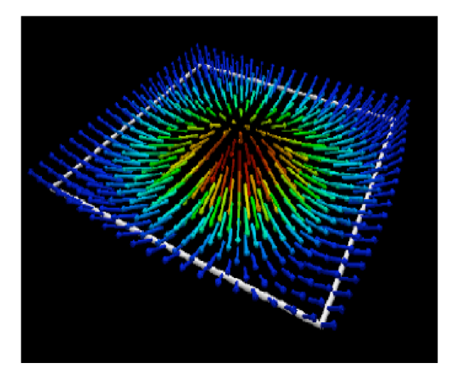
Figure 2: Distribution of spins  in a skyrmion

The presence of skyrmions was predicted theoretically and convincingly proved experimentally for two-dimensional electron gas in the condition of the Quantum Hall Effect. Theoretical prediction was made by Sondhi et al. [16]. They argued that the exchange interaction between electrons is sufficiently large to make this system almost ideal ferromagnet. The Zeeman energy is relatively small due to smallness of the gyromagnetic factor, which can be reduced almost to zero by a comparatively small hydrostatic pressure. The direct Coulomb interaction is also small in comparison to the exchange, but it fixes the radius of the Skyrmion. In contrast to the case of the Heisenberg ferromagnet the Skyrmion carries electric charge. These localized objects has rather big spin proportional to its area. Participating in the process of the spin relaxation in the NMR it increases dramatically the relaxation time. Another effect is a sharp peak in the dynamic spin polarization due to Skyrmions (see Fig. 3). The NMR measurements were performed with the heterojunction Ga/GaAs/GaAlAs.

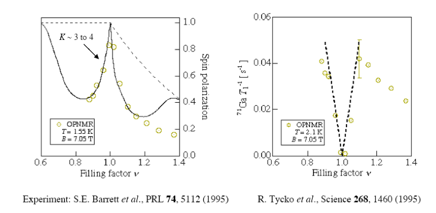
Figure 3: The left panel shows the spin polarization in the NMR experiment near the filling factor $\nu=1$; the right panel shows the NMR relaxation rate vs. the filling factor.

These experiments allow to estimate the skyrmion radius or the total spin of the skyrmion $S\approx 16$. Many theoretical works were dedicated to study of the phase diagram: do the skyrmion form a liquid gas or a crystal structure and what is the magnetic state of the system as a whole (see, for example [17]), but experimentally it is not yet well established.

Indirect evidences of the skyrmion presence in antiferromagnets were indicated by F. Waldner [18]. He analyzed three types of experiments: elastic neutron scattering for quasi-two dimensional compounds NTT [19] and Rb₂Mn_xCr_1-xCl₄ [20] which gives the value of the correlation length vs. temperature; the line broadening in the electron spin resonance (ESR) in several quasi-two-dimensional compounds like (CH₂)₂(NH₃)₂MnCl₄ and similar organic magnets, K₂MnF₄ and Rb₂MnF₄ [21]; the NMR relaxation rate in some of these compounds [22]. In all cases he found the activation exponent with the barrier energy equal to $AJS^{2}$ with the numerical coefficient $A=4\pi$ within the precision of the experiment.

Why the skyrmion were not observed in weakly anisotropic ferromagnetic films as permalloy, Fe and Ni on a smooth crystal substrate? The reason was elucidated in the work [23]. The authors studied what happens with the skyrmion at small symmetry-breaking perturbations like anisotropy, magnetic field or dipolar forces. Their conclusion is that the uniaxial anisotropy itself leads to shrinking of the skyrmion to zero radius. However, if the 4-order in derivatives term in the exchange interaction is positive, it makes the skyrmion stable and fixes it radius $R\sim\sqrt{l_{dw}a}$, where $l_{dw}$ is the domain wall width and $a$ is the lattice constant. For real magnets this radius varies between 1 and 10 nm. This is a very small object and its experimental observation requires very high resolution. Theory predicts that in ferromagnetic insulators with localized spins the sign of the mentioned correction to the exchange interaction is negative unless the couplings between not-nearest neighbors are anomalously large. Thus, skyrmions are absolutely unstable in these ferromagnets. In the itinerant ferromagnets with the oscillating RKKY interaction between spins, the sign is positive and we can expect stable, but very small skyrmions. This is a disadvantage for their experimental discovery, but may be very useful in their application as digits in a magnetic record.

Last several years experimentalists proposed a modification of the skyrmion [24]. They deposit permalloy magnetic disks with the radius from 0.1 to 1 $\mu m$. The dipolar forces in such a disk put the spins into the plane. At small radius the monodomain configuration with all spins parallel (in-plane) is energetically stable, but at larger radius the vortex configuration wins everywhere except of a small circle near the center where spins go out of plane exactly as in skyrmion. The radius of this pseudoskyrmion is $\sim\sqrt{J/M^{2}d}$, where $d$ is the thickness of the disk. Despite of the seeming likeness between this problem and problem of skyrmion the shape of this excitation is rather different from that of the skyrmion.

3.2 Instantons

The first classical instanton solution in the gauge field theory was obtained by Belavin, Polyakov, Schwarz and Tyupkin in 1975 [25]. It represents a limited in time tunneling trajectory between two topologically different vacuum states. In condensed matter physics such transitions are frequent phenomena. In some situations they represent a dominant mechanism of dissipation. We will describe couple of such cases.

3.2.1 Phase slip centers

The phase slip centers were proposed by Skocpol, Beasley and Tinkham [26] as a mechanism of dissipation in thin superconducting wires. Small transverse sizes of such wires make impossible the formation of vortices and suppress the motion of normal carriers (quasiparticles). The paradox is that the electric field penetrating in the wires should accelerate the Cooper pairs and destroy the superconducting state. Instead they proposed that a new node of the condensate (Ginzburg-Landau) wave function enters into a wire. The phase changes by 2$\pi$ at passing such a center. This is the so-called phase-slip center. Since it moves inside the wire, the phase changes with time. According to Josephson the time dependent phase generates a voltage and together with it dissipation.

Ivlev and Kopnin [27] were the first to recognize that the phase-slip centers are typical instantons. The change of the phase by $2\pi$ can be treated as a transition to a vacuum with another topological number. The field and phase at a  fixed point is time-dependent and also changes from point to point. To ensure a state stationary in average the phase and field variations must be periodic both in time and in space. Thus, the phase-slip centers form a regular  rectangular lattice in the space-time plane (see Fig. 4) and physical values are double periodic.

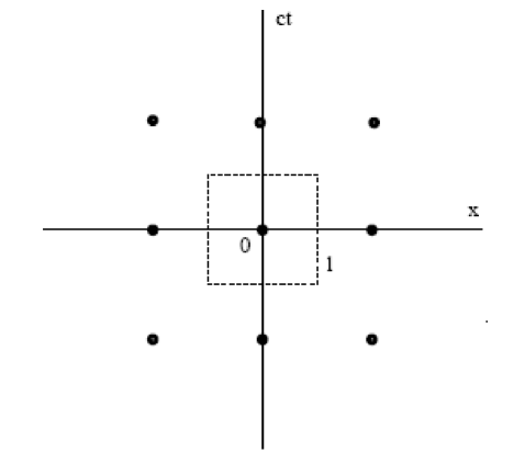
Figure 4: The lattice of phase-slip centers in space-time plane. The contour $l$ encircles a unit cell of the lattice.

Ivlev and Kopnin proposed a ”quantization rule” for the electric field in the two-dimensional space time $x_{0}=ct$, $x_{1}=x$. They introduced the gauge-invariant potentials $\mathbf{Q=A-}\frac{\hbar c}{2e}\nabla\chi$ and $\Phi=\varphi+\frac{\hbar}{2e}\frac{\partial\chi}{\partial t}$, where $\mathbf{A}$ is the electromagnetic vector-potential, $\varphi$ is the scalar potential and $\chi$ is the phase of the condensate wave function. In the wire only a component along the wire $Q_{x}$ survives. Let introduce relativistically-covariant 2-component vector $\mathbf{q=}\left(\Phi_{x},Q\right)$ and consider its circulation around a contour $l$ surrounding a phase-slip center and containing an elementary cell of the lattice. Since the vector $\mathbf{q}$ has the periodicity of the lattice, this circulation is equal to zero. The vector $\mathbf{q}$ can be represented in terms of the standard ”relativistic” 2-vector-potential $\mathbf{a=(\varphi,A})$ and the 2-gradient of the phase: $\mathbf{q=a-}\frac{\hbar c}{2e}\nabla\chi$. Zero circulation of the vector $\mathbf{q}$ implies that ${\displaystyle\oint}\mathbf{a\cdot}d\mathbf{r=\Phi}_{0}n;$ where $\leavevmode\nobreak\ \mathbf{\Phi}_{0}=\frac{\pi\hbar c}{e}$ is the (superconducting) flux quantum and $n$ is an integer. Using the Stokes theorem and the expression of electric field via potentials, they found:

$${\displaystyle\int\nolimits_{c}}Edxcdt=\mathbf{\Phi}_{0}n$$ (3.1)

This equation determines the average electric field $\bar{E}$ in terms of repeating phase-slip frequency $\omega$ and the distance between them $L$: $\bar{E}=\frac{\hbar\omega}{2eL}$. In the dc regime the current drops each time when the number of phase-slip centers in the wire changes by one. Discontinuous current-voltage curves were first obtained in the experiment by Skocpol et al. [26]. In Fig. 5. we show the current voltage characteristics extracted from the work by Jelia et al. [28].

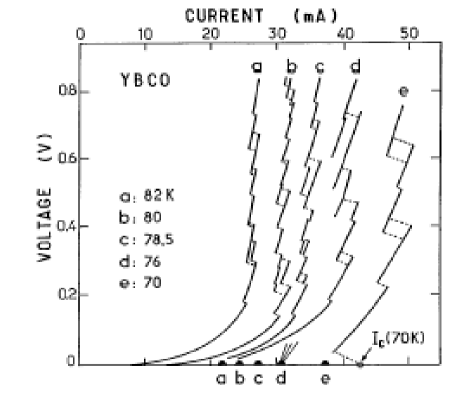
Figure 5: dc current-voltage characteristics of an YBCO bridge (length 200 $\mu$m, width 20 $\mu$m, thickness 90 nm) showing jumps of the current and resistance.

The resonance with an external ac radiation of proper frequency results in Shapiro steps in current  voltage characteristics of superconducting wires as it is shown on Fig. 6.

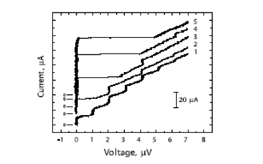
Figure 6: Current-voltage characteristics of a 15 $\mu$m wide Sn strip under microwave irradiation with frequency $f$ 0.5 GHz (1), 1 GHz (2), 2 GHz (3), 3GHz (4), no microwaves (5). The graph is extracted from the article by Sivakov et al. [29]

Phase-slip centers appear also in one-dimensional or quasi-one-dimensional charge density waves (CDW) [30]. Charge density waves are described by a scalar complex order parameter. The change of its phase by $2\pi$ is the instanton and has the same structure as in superconductors, but its physical manifestation is different: it is caused by a voltage bias and causes the charge transfer, i.e. the current. Therefore, in corresponding I-V characteristics the current and voltage interchange each other in comparison to the corresponding characteristics for superconductors.

4 Thermodynamics of membranes

In 1981 Polyakov made a fundamental work in the quantum string theory [31]. He described their propagation as a random surface in which not only the shape of the surface, but also the metrics fluctuates. In his work [31] Sasha indicated the simple and reliable way for practical computation of statistics: the triangulation of surfaces. Besides of its direct impact on the string theory and quantum gravitation, it had a deep influence onto statistical physics of membranes, in particular biological membranes. Two reasons enforce me to be brief in this section: the formalism is more complicated than in others sections and I am far from being an expert in this problem. Therefore I will not try to reproduce complicated fluctuating differential geometry. Instead I refer the reader to original articles. However, we show some pictures to give the feeling what it is about. One of the most important problems of this theory is the so-called crumpling transition, i.e. the transition from a compact comparatively smooth state of the membrane to a fractional state with sharp edges and peaks like in a roughly folded sheet of paper [32]. In a later work [33] Sasha indicated an useful analogy between the Heisenberg model and his model of quantum surface: the normals to the surface play the role of spins. The smooth state is analogous to a ferromagnet, whereas the crumpled state is an analogue of a paramagnet. On Fig. 6,7 we illustrate this transition by computational pictures extracted from the P.Coddington’s website http://www.cs.adelaide.edu.au/users/paulc/physics/randomsurfaces.html.

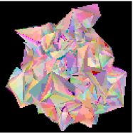
Figure 7: The smooth state of a membrane

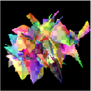
Figure 8: The crumpled state of a membrane.

In a real experiment with the DMPC membranes (DMPC is an abbreviation for dimyristol phosphatidylchlorine) the difference in shape looks not less dramatic (see Fig. 8). The transition is driven with concentration of a special reagent farnesol [34].

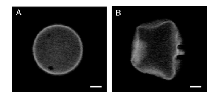
Figure 9: A DCMP vesicle before and after the crumpling transition. The scale represents 5 $\mu$m. The transition proceeds at 20% of the farnesol at 13⁰C.

Abstract

Straightforward evaluation of the correlation functions in 2D minimal gravity requires integration over the moduli space. For degenerate fields the higher equations of motion of the Liouville field theory allow to turn the integrand to a derivative and to reduce it to the boundary terms and the so-called curvature contribution. The last is directly related to the expectation value of the corresponding ground ring element. The action of this element on a cohomology related to a generic matter primary field is evaluated directly through the operator product expansions of the degenerate fields. This permits us to construct the ground ring algebra and to evaluate the curvature term in the four-point function. The operator product expansions of the Liouville “logarithmic primaries” are also analyzed and relevant logarithmic terms are carried out. All this results in an explicit expression for the four-point correlation number of one degenerate and three generic matter fields. We compare this integral with the numbers coming from the matrix models of 2D gravity and discuss some related problems and ambiguities.

1 Introduction

1. Liouville gravity (LG) is the term for the two-dimensional quantum gravity whose action is induced by a “critical” matter, i.e., the matter described by a conformal field theory (CFT) $\mathcal{M}_{c}$ with central charge $c$. This induced action is universal and is called the Liouville action, because its variation with respect to the metric is proportional to the Liouville (or constant curvature) equation [1]. Let us denote $\left\{\Phi_{i},\Delta_{i}\right\}$ be the set of primary fields and their dimensions in $\mathcal{M}_{c}$.

2. Liouville field theory (LFT) is constructed as the quantized version of the classical theory based on the Liouville action. LFT is again a conformal field theory with central charge $c_{\text{L}}$. It is convenient to parameterize it in terms of variable $b$ or

$$Q=b^{-1}+b$$ (1.1)

as

$$c_{\text{L}}=1+6Q^{2}$$ (1.2)

Parameter $b$ enters the local Lagrangian

$$\mathcal{L}_{\text{L}}=\frac{1}{4\pi}\left(\partial_{a}\phi\right)^{2}+\mu e^{2b\phi}$$ (1.3)

where $\mu$ is the scale parameter called the cosmological constant and $\phi$ is the dynamical variable for the quantized metric

$$ds^{2}=\exp\left(2b\phi\right)\widehat{g}_{ab}dx^{a}dx^{b}$$ (1.4)

Here $\widehat{g}_{ab}$ is the “reference metric”, a technical tool needed to give LFT a covariant form

$$\mathcal{A}_{\text{L}}=\int\left(\frac{1}{4\pi}\widehat{g}^{ab}\partial_{a}\phi\partial_{b}\phi+\frac{Q}{4\pi}\phi\widehat{R}+\mu e^{2b\phi}\right)\sqrt{\widehat{g}}d^{2}x$$ (1.5)

with $\widehat{R}$ the scalar curvature of the background metric. Basic primary fields are the exponential operators $V_{a}=\exp\left(2a\phi\right)$, parameterized by a continuous (in general complex) parameter $a$ in the way that the corresponding conformal dimension is

$$\Delta_{a}^{\text{(L)}}=a(Q-a)$$ (1.6)

Liouville field theory is exactly solvable [2]. In particular the three-point function $C_{\text{L}}(a_{1},a_{2},a_{3})=\left\langle V_{a_{1}}(x_{1})V_{a_{2}}(x_{2})V_{a_{3}}(x_{3})\right\rangle_{\text{L}}$ is known explicitly for arbitrary exponential fields

$$C_{\text{L}}(a_{1},a_{2},a_{3})=\left(\pi\mu\gamma(b^{2})b^{2-2b^{2}}\right)^{(Q-a)/b}\frac{\Upsilon_{b}(b)}{\Upsilon_{b}(a-Q)}\prod_{i=1}^{3}\frac{\Upsilon_{b}(2a_{i})}{\Upsilon_{b}(a-a_{i})}$$ (1.7)

where $a=a_{1}+a_{2}+a_{3}$ and $\Upsilon_{b}(x)$ is a special function related to the Barnes double gamma function (see e.g. [3]). Correlation function (1.7) is consistent with the following identification of the exponential fields with different values of $a$

$$V_{a}(x)=R_{\text{L}}(a)V_{Q-a}(x)$$ (1.8)

known as the reflection relations [3]. Here

$$R_{\text{L}}(a)=\left(\pi\mu\gamma(b^{2})\right)^{(Q-2a)/b}\frac{\gamma(2ab-b^{2})}{\gamma(2-2ab^{-1}+b^{-2})}$$ (1.9)

is called the Liouville reflection amplitude. The local structure of LFT is determined completely by the general “continuous” operator product expansion (OPE) of generic Liouville exponential fields

$$V_{a_{1}}(x)V_{a_{2}}(0)=\int^{\prime}\frac{dP}{4\pi}C_{a_{1},a_{2}}^{\text{(L)}Q/2+iP}(x\bar{x})^{\Delta_{Q/2+iP}^{\text{(L)}}-\Delta_{a_{1}}^{\text{(L)}}-\Delta_{a_{2}}^{\text{(L)}}}\left[V_{Q/2+iP}(0)\right]$$ (1.10)

where the structure constant is expressed through (1.7) $C_{a_{1},a_{2}}^{\text{(L)}p}=$ $C_{\text{L}}(g,a,Q-p).$ The integration contour here is the real axis if $a_{1}$ and $a_{2}$ are in the “basic domain”

$$\left|Q/2-\operatorname*{Re}a_{1}\right|+\left|Q/2-\operatorname*{Re}a_{2}\right|<Q/2$$ (1.11)

In other domains of these parameters an analytic continuation is implied. It is equivalent to certain deformation of the contour due to the singularities of the structure constant. This prime near the integral sign helps to keep in mind this prescription.

In LG the parameter $b$ is chosen in the way that together with $\mathcal{M}_{c}$ LFT forms a joint conformal field theory with central charge $c+c_{\text{L}}=26$. Technically it is also convenient to include the

3. Reparametrization ghost field theory. This is the standard fermionic $BC$ system of spin $(2,-1)$

$$A_{\text{gh}}=\frac{1}{\pi}\int(C\bar{\partial}B+\bar{C}\partial\bar{B})d^{2}x$$ (1.12)

with central charge $-26$, which corresponds to the gauge fixing Faddeev-Popov determinant. The matter+Liouville stress tensor $T$ is a generator of $26$ dimensional Virasoro algebra. Together with the ghost field theory this allows to form a BRST complex with respect to the nilpotent BRST charge

$$\mathcal{Q}=\oint\left(CT+C\partial CB\right)\frac{dz}{2\pi i}$$ (1.13)

4. Correlation functions is one of the most important problems in the LG. In gravitational correlation functions the matter operators $\Phi_{i}$ are “dressed” by appropriate exponential Liouville fields $V_{a_{i}}$ in the way to form either the $(1,1)$ form $U_{i}=\Phi_{i}V_{a_{i}}$ of ghost number $0$ or the dimension $(0,0)$ operator $W_{i}=C\bar{C}U_{i}$ of ghost number $1$. In both cases this requires

$$\Delta_{i}+a_{i}(Q-a_{i})=1$$ (1.14)

Invariant (or integrated) correlation functions are independent on any coordinates and better called the correlation numbers. In the field theoretic framework, a (genus $0$) correlation number $\left\langle U_{1}\ldots U_{n}\right\rangle_{\text{G}}$ at $n\geq 3$ is constructed as the integral

$$\left\langle U_{1}\ldots U_{n}\right\rangle_{\text{G}} =\int_{M_{n}}\left\langle W_{1}(x_{1})\ldots W(x_{n})\right\rangle$$ (1.15)

$$=\int\left\langle W_{1}(x_{1})W_{2}(x_{2})W_{3}(x_{3})U_{4}(x_{4})d^{2}x_{4}\dots U(x_{n})d^{2}x_{n}\right\rangle$$

The integration here is over the moduli space $M_{n}$ of the sphere with $n$ punctures. Technically it is equivalent to choose any $3$ of $W_{i}$ at arbitrary fixed positions $x_{1}$, $x_{2}$ and $x_{3}$ and integrate the $(1,1)$ forms $U_{i}(x_{i})d^{2}x_{i}$ inserted instead of $W_{i}$ at $i=4,\ldots,n$. At $n<3$ the definition is slightly different. This is because of non-trivial conformal symmetries of the sphere with $2$ and $0$ punctures.

The simplest case of 1.15 is the tree-point function, where the moduli space is trivial and the result is factorized in a product of the matter, Liouville and ghost three-point functions

$$\left\langle U_{1}U_{2}U_{3}\right\rangle_{\text{G}}=x_{12}\bar{x}_{12}x_{23}\bar{x}_{23}x_{31}\bar{x}_{31}\left\langle\Phi_{1}(x_{1})\Phi_{2}(x_{2})\Phi_{3}(x_{3})\right\rangle_{\text{CFT}}\left\langle V_{1}(x_{1})V_{2}(x_{2})V(x_{3})\right\rangle_{\text{L}}$$ (1.16)

The three-point functions $\left\langle\Phi_{1}(x_{1})\Phi_{2}(x_{2})\Phi_{3}(x_{3})\right\rangle_{\text{CFT}}$, familiar also as the structure constants of the operator product expansion (OPE) algebra, are known explicitly in solvable matter CFT’s. Thus eq.(1.16) gives the LG 3-point correlation number in the explicit form. The two-point number and the zero-point one (the partition sum) are simply read off from this expression of the 3-point function.

5. The four-point function is the next step in the order of complexity

$$\ \left\langle U_{1}U_{2}U_{3}U_{4}\right\rangle_{\text{G}} =$$ (1.17)

$$\ x_{12}\bar{x}_{12}x_{23}\bar{x}_{23}x_{31}\bar{x}_{31}\int\left\langle\Phi_{1}(x_{1})\ldots\Phi_{4}(x_{4})\right\rangle_{\text{CFT}}\left\langle V_{1}(x_{1})\ldots V_{4}(x_{4})\right\rangle_{\text{L}}d^{2}x_{4}$$

This expression is much less explicit. First, it involves the integration over $x_{4}$. Then, even if the matter 4-point function is known in any convenient form, general representations for the Liouville four-point function are more complicated. E.g., the “conformal block” decomposition [3]

$$\left\langle V_{1}(x_{1})\ldots V_{4}(x_{4})\right\rangle_{\text{L}} =$$ (1.18)

$$\int\frac{dP}{4\pi}C_{\text{L}}(a_{1},a_{2},Q/2+iP)C_{\text{L}}(Q/2-iP,a_{3},a_{4})\mathcal{F}_{P}(a_{i},x_{i})\mathcal{F}_{P}(a_{i},\bar{x}_{i})$$

involves the so called general conformal block [4]

$$\mathcal{F}_{P}(a_{i},x_{i})=\raisebox{-26.68881pt}{\includegraphics[height=59.18913pt,width=104.06125pt]{block.eps}}=\mathcal{F}_{P}\left(\left.\begin{array}[c]{cc}a_{1}&a_{3}\\ a_{2}&a_{4}\end{array}\right|\begin{array}[c]{cc}x_{1}&x_{3}\\ x_{2}&x_{4}\end{array}\right)$$ (1.19)

which is by itself a complicated function of its arguments, not to talk about the integration over the “intermediate momentum” $P$ in (1.18). In the present paper we take a preliminary step towards the evaluation of the four-point integral in the special case of

6. Minimal gravity (MG). If the conformal matter $\mathcal{M}_{c}$ is represented by a minimal CFT model (more precisely, a “generalized minimal model” (GMM), see below) $\mathcal{M}_{b^{2}}$, we talk about the “minimal gravity” (MG) (respectively generalized minimal gravity (GMG)). In GMG the evaluation of the four-point integral is dramatically simplified in the case when one of the matter operators $\Phi_{i}$ in the r.h.s. of (1.17) is a degenerate field $\Phi_{m,n}$. This is due to the so called “higher equations of motion” (HEM) which hold for the operator fields in LFT [5]. Let $U_{4}=U_{m,n}$ where

$$U_{m,n}=\Phi_{m,n}\tilde{V}_{m,n}$$ (1.20)

and $\tilde{V}_{m,n}$ is an appropriate Liouville dressing for $\Phi_{m,n}$. Then HEM’s allow to rewrite the integrand in (1.17) as a derivative

$$\ \left\langle U_{1}U_{2}U_{3}U_{m,n}\right\rangle_{\text{GMG}}=B_{m,n}^{-1}\int\partial\bar{\partial}\left\langle O_{m,n}^{\prime}(x)W_{1}(x_{1})W_{2}(x_{2})W_{3}(x_{3})\right\rangle d^{2}x$$ (1.21)

($B_{m,n}$ is a numerical constant, see sect.3) and hence reduce the problem to the boundary terms and the so-called curvature term. The last is directly expressed in terms of the expectation value $\left\langle O_{m,n}W_{1}W_{2}W_{3}\right\rangle$ of the

7. Ground ring (GR) element $O_{m,n}$ associated with the field $\Phi_{m,n}$. Therefore, we want to learn handle the ground ring algebra and the correlation functions of its elements. This knowledge will also prove instructive in the subsequent calculations of the

8. Boundary terms. To evaluate the boundary contributions we need to know appropriate terms in the OPE of the field $O_{m,n}^{\prime}$ in (1.21). This field is constructed as a “logarithmic counterpart” of the element $O_{m,n}$ and satisfies the identity

$$\partial\bar{\partial}O_{m,n}^{\prime}=B_{m,n}U_{m,n}+\text{BRST exact}$$ (1.22)

Analysis of this expansion allows to evaluate the boundary contributions and finally the four-point integral (1.17) with $U_{4}=U_{m,n}$. This is the main purpose of all the work presented below.

2 Generalized minimal models

Strictly speaking, minimal models of CFT $\mathcal{M}_{p/p^{\prime}}$ [4] are consistently defined as a field theoretic constructions only if the “parameter” $p/p^{\prime}$ is an irreducible rational number so that $p$ and $p^{\prime}$ are coprime integers. In this case the finite set of $(p-1)(p^{\prime}-1)/2$ degenerate primary fields $\Phi_{m,n}$ with $1\leq m<p$ and $1\leq n<p^{\prime}$ (modulo the identification $\Phi_{m,n}=\Phi_{p-m,p^{\prime}-n}$) form, together with their irreducible representations, the whole space of $\mathcal{M}_{p/p^{\prime}}$. “Canonical” minimal models $\mathcal{M}_{p/p^{\prime}}$ are believed to be a completely consistent CFT, i.e., to satisfy all standard requirements of quantum field theory, except for (in most cases) the unitarity. They are also considered exactly solvable as the structure of their OPE algebra is known explicitly [6].

There are many ways to relax some of the requirements leading to the set of $\mathcal{M}_{p/p^{\prime}}$ as unique CFT structures. For example, in the literature the “parameter” $p/p^{\prime}$ is often taken as an arbitrary number (e.g., [6]). The algebra of the degenerate primary fields doesn’t close any more within any finite subset and rather the whole set $\{\Phi_{m,n}\}$ with $(m,n)$ any natural numbers forms a closed algebra. Moreover, some authors include local fields with dimensions different from the Kac values, even continuous spectrum of dimensions. Although the consistency of such constructions from the field theoretic point of view remains to be clarified, these extensions prove to be a convenient technical tool. Moreover, statistical mechanics offers a number of examples where either a generalization of $\mathcal{M}_{p/p^{\prime}}$ for non-integer values $p/p^{\prime}$ is essentially necessary or non-degenerate primary operators appear as observables (both generalization are sometimes required).

In this paper we denote $b^{2}$ the parameter $p/p^{\prime}$ and admit the notion of GMM in the most wide sense as a conformal field theory with central charge

$$c=1-6(b^{-1}-b)^{2}$$ (2.1)

which may involve fields $\Phi_{\alpha}$ of any dimension. Continuous parameter $\alpha$ is introduced to parameterize a continuous family of primary fields with dimensions

$$\Delta_{\alpha}^{\text{(M)}}=\alpha(\alpha-q)$$ (2.2)

where

$$q=b^{-1}-b$$ (2.3)

Also we always use the “canonical” CFT normalization of the primary fields $\Phi_{\alpha}$ through the two-point functions

$$\left\langle\Phi_{\alpha}\Phi_{\alpha}\right\rangle_{\text{GMM}}=\left(x\bar{x}\right)^{-2\Delta_{\alpha}}$$ (2.4)

Degenerate fields $\Phi_{m,n}$ have dimensions

$$\Delta_{m,n}^{\text{(M)}}=-q^{2}/4+\lambda_{m,-n}^{2}$$ (2.5)

where yet another convenient notation

$$\lambda_{m,n}=(mb^{-1}+nb)/2$$ (2.6)

is introduced. They correspond to either $\alpha=\alpha_{m,n}$ or $\alpha=q-\alpha_{m,n}$ with

$$\alpha_{m,n}=q/2+\lambda_{-m,n}$$ (2.7)

The main restrictions, which singles out this apparently loose construction, is that the

1. Degenerate fields $\Phi_{1,2}$ and $\Phi_{2,1}$ (and therefore in general the whole set $\left\{\Phi_{m,n}\right\}$) are in the spectrum

2. The null-vectors in the degenerate representations $\Phi_{m,n}$ vanish

$$D_{m,n}^{\text{(M)}}\Phi_{m,n}=\bar{D}_{m,n}^{\text{(M)}}\Phi_{m,n}=0$$ (2.8)

Here $D_{m,n}^{\text{(M)}}$ ($\bar{D}_{m,n}^{\text{(M)}}$) are the operators made of the right Virasoro generators $M_{n}$ (respectively left $\bar{M}_{n}$) which create the level $mn$ singular vector in the Virasoro module of $\Phi_{m,n}$. For definiteness we normalize these operators through the $M_{-1}^{mn}$ term as

$$D_{m,n}^{\text{(M)}}=M_{-1}^{mn}+d_{1}^{(m,n)}(b^{2})M_{-2}M_{-1}^{mn-2}+\ldots$$ (2.9)

   First examples read explicitly

$$D_{1,2}^{\text{(M)}} =M_{-1}^{2}-b^{2}M_{-2}$$ (2.10)

$$D_{1,3}^{\text{(M)}} =M_{-1}^{3}-2b^{2}(M_{-2}M_{-1}+M_{-1}M_{-2})+4b^{4}M_{-3}$$

$$\ldots$$

3. The identification $\Phi_{\alpha}\equiv\Phi_{q-\alpha}$ is also often added.

It turns out that this set of definitions imposes important restrictions on the structure of this formal construction. The three-point function

$$C_{\text{M}}(\alpha_{1},\alpha_{2},\alpha_{3})=\left\langle\Phi_{\alpha_{1}}\Phi_{\alpha_{2}}\Phi_{\alpha_{3}}\right\rangle_{\text{GMM}}$$ (2.11)

of the “generic” primary fields can be restored uniquely from the above requirements [7]

$$C_{\text{M}}(\alpha_{1},\alpha_{2},\alpha_{3})=\frac{b^{b^{-2}-b^{2}-1}\Upsilon_{b}(2b-b^{-1}+\alpha)}{\left[\gamma(1-b^{2})\gamma(2-b^{-2})\right]^{1/2}\Upsilon_{b}(b)}\prod_{i=1}^{3}\frac{\Upsilon_{b}(\alpha-2\alpha_{i}+b)}{\left[\Upsilon_{b}(2\alpha_{i}+b)\Upsilon_{b}(2\alpha_{i}+2b-b^{-1})\right]^{1/2}}$$ (2.12)

where again $\alpha=\alpha_{1}+\alpha_{2}+\alpha_{3}$ and $\Upsilon_{b}(x)$ is the same function as in eq.(1.7). At the degenerate values of the parameters $\alpha_{i}=\alpha_{m_{i},n_{i}}$ (and if the standard “fusion” relations are satisfied) the known degenerate structure constants [6] are recovered from (2.12).

Explicit form of the OPE of $\Phi_{1,2}$ and a generic primary field $\Phi_{\alpha}$

$$\Phi_{1,2}(x)\Phi_{\alpha}(0)=C_{+}^{\text{(M)}}(\alpha)(x\bar{x})^{\alpha b}\left[\Phi_{\alpha+b/2}\right]+C_{-}^{\text{(M)}}(\alpha)(x\bar{x})^{1-\alpha b-b^{2}}\left[\Phi_{\alpha-b/2}\right]$$ (2.13)

($\left[\Phi_{\alpha}\right]$ stands for a primary field $\Phi_{\alpha}$ and all the tower of its conformal descendants) will be of use below. In our normalization

$$C_{+}^{\text{(M)}}(\alpha)=\left[\frac{\gamma(b^{2})\gamma(2\alpha b+2b^{2}-1)}{\gamma(2b^{2}-1)\gamma(b^{2}+2\alpha b)}\right]^{1/2}\;;\;\;C_{-}^{\text{(M)}}(\alpha)=\left[\frac{\gamma(b^{2})\gamma(2\alpha b+b^{2}-1)}{\gamma(2b^{2}-1)\gamma(2\alpha b)}\right]^{1/2}$$ (2.14)

General form of (2.13) reads

$$\Phi_{m,n}(x)\Phi_{\alpha}(0)=\sum_{r,s}^{(m,n)}\left(x\bar{x}\right)^{\lambda_{r,s}(2\alpha+\lambda_{r,s}-q)-\Delta_{m,n}^{\text{(M)}}}C_{\text{M}}(\alpha_{m,n},\alpha,\alpha+\lambda_{r,s}))\left[\Phi_{\alpha+\lambda_{r,s}}\right]$$ (2.15)

where $\lambda_{r,s}$ are as in eq.(2.6) and the sign $\sum_{r,s}^{(m,n)}$ stands for the sum over the following set of integers (we use the notation $\{n_{1}:d:n_{1}+nd\}=\{n_{1},n_{1}+d,\ldots,n_{1}+nd\}$)

$$(r,s)=(\{-m+1:2:m-1\},\{-n+1:2:n-1\})$$ (2.16)

Other exact results in GMM form somewhat miscellaneous collection. What is important for our program is the construction of the four-point function

$$G_{(m,n),\alpha_{1},\alpha_{2},\alpha_{3}}^{\text{(GMM)}}(x)=\left\langle\Phi_{m,n}(x)\Phi_{\alpha_{1}}(x_{1})\Phi_{\alpha_{2}}(x_{2})\Phi_{\alpha_{3}}(x_{3})\right\rangle_{\text{GMM}}$$ (2.17)

with one degenerate field $\Phi_{m,n}$ and three generic primaries $\Phi_{\alpha}$[4]. The null-vector decoupling condition (2.8) entails certain partial differential equation for the corresponding correlations functions. In the four-point case this equation reduces to an ordinary linear differential equation of the order $mn$, whose independent solutions are the four-point conformal blocks (in the picture we denote $\Delta_{i}=\Delta_{\alpha_{i}}^{\text{(M)}}$ and $\Delta_{m,n}=\Delta_{m,n}^{\text{(M)}}$)

$$\mathcal{F}_{r,s}(x)=\raisebox{-41.12164pt}{\includegraphics[height=87.68538pt,width=178.8753pt]{rsblock.eps}}$$ (2.18)

and $\Delta_{(r,s)}=\Delta_{\alpha_{1}}^{\text{(M)}}+\lambda_{r,-s}\left(2\alpha_{1}-q+\lambda_{r,-s}\right)$. The four point function is then combined as

$$G_{(m,n),\alpha_{1},\alpha_{2},\alpha_{3}}^{\text{(GMM)}}(x)=$$ (2.19)

$$\sum_{r,s}^{(m,n)}C_{\text{M}}(\alpha_{m,n},\alpha_{1},\alpha_{1}+\lambda_{r,-s})C_{\text{M}}(\alpha_{1}+\lambda_{r,-s},\alpha_{2},\alpha_{3})\mathcal{F}_{r,s}(x)\mathcal{F}_{r,s}(\bar{x})$$

where $\sum_{r,s}^{(m,n)}$ has the same meaning as in eq.(2.15).

The following remark is very relevant for the subsequent developments. In the present study, when considering the GMG, we restrict ourselves only to the four point function with one degenerate matter field $\Phi_{m,n}$, leaving the other three to be formal generics $\Phi_{\alpha}$. In particular, expression (2.19) is the relevant construction for the matter part of the integrand in eq.(1.17). What is important is that if one or more of the operators $\Phi_{\alpha}$ are also degenerate, the number of conformal blocks entering the correlation function (2.19) might be reduced and this expression doesn’t hold literally. In this case the considerations below are not literally valid. Important and sometimes rather subtle modifications has to be made. In the present paper we will not study this interesting but more delicate situation (although it is extremely actual in quantum gravity applications).

There is another interesting aspect similar to the subtlety mentioned above. When dealing with GMM one should keep in mind that there are objects of different nature. Some are continuous in the parameter $b^{2}$, like the central charge, degenerate dimensions or certain correlation functions. Others may be highly discontinuous and dependent on the arithmetic nature of the numbers $p$ and $p^{\prime}$. Simplest example is the number of irreducible Virasoro representations entering the theory. This warns us to be careful when trying to reproduce the results of $\mathcal{M}_{p/p^{\prime}}$ as a naive limit of $\mathcal{M}_{b^{2}}$ as $b^{2}\rightarrow p/p^{\prime}$ and $\alpha\rightarrow\alpha_{m,n}$ in the formal primary fields. This is why we stress again that the three matter fields $\Phi_{\alpha}$ in the matter correlation function have generic non-degenerate values of the parameters $\alpha_{1}$, $\alpha_{2}$ and $\alpha_{3}$.

3 Higher equations of motion

Let $a_{m,n}=Q/2-\lambda_{m,n}$ with $(m,n)$ a pair of positive integers, so that $V_{m,n}=V_{a_{m,n}}$ are the Liouville exponentials corresponding to degenerate representations of the Liouville Virasoro algebra. Let also $D_{m,n}^{\text{(L)}}$ be the corresponding “singular vector creating” operators made of the Liouville Virasoro generators $L_{n}$, similar to the operators $D_{m,n}^{\text{(M) }}$ introduced above. In fact $D_{m,n}^{\text{(L)}}$ is obtained from $D_{m,n}^{\text{(M)}}$ through the substitution $M_{n}\rightarrow L_{n}$ and $b^{2}\rightarrow-b^{2}$. Like in GMM, in LFT the corresponding singular states vanish [8, 9]

$$D_{m,n}^{\text{(L)}}V_{m,n}=\bar{D}_{m,n}^{\text{(L)}}V_{m,n}=0$$ (3.1)

Let $D_{m,n}^{\text{(L)}}$ be normalized similarly to (2.9) as

$$D_{m,n}^{\text{(L)}}=L_{-1}^{mn}+d_{1}^{(m,n)}(-b^{2})L_{-2}L_{-1}^{mn-2}+\ldots$$ (3.2)

Define also the “logarithmic degenerate” fields

$$V_{m,n}^{\prime}=\frac{1}{2}\frac{\partial}{\partial a}V_{a}|_{a=a_{m,n}}$$ (3.3)

for every pair $(m,n)$ of natural numbers. These fields are not primary. Under conformal transformations $x\rightarrow y$ they transform as

$$\left|y_{x}\right|^{2\Delta_{m,n}}V_{m,n}^{\prime}(y)=V_{m,n}^{\prime}(x)-\Delta_{m,n}^{\prime}V_{m,n}(x)\log\left|y_{x}\right|$$ (3.4)

where $y_{x}$ stands for $\partial y/\partial x$. Nevertheless, as it is shown in [5] $D_{m,n}^{\text{(L)}}\bar{D}_{m,n}^{\text{(L)}}V_{m,n}^{\prime}$ is a primary field and, moreover, the following identity holds for the LFT operator fields

$$D_{m,n}^{\text{(L)}}\bar{D}_{m,n}^{\text{(L)}}V_{m,n}^{\prime}=B_{m,n}\tilde{V}_{m,n}$$ (3.5)

where $\tilde{V}_{m,n}=V_{a}|_{a=a_{m,-n}}$ is the Liouville exponential of dimension $\Delta_{m,n}^{\text{(L)}}+mn$. The numerical constant $B_{m,n}$ reads

$$B_{m,n}=\frac{\left(\pi\mu\gamma(b^{2})\right)^{n}b^{1+2n-2m}}{\gamma(1-m+nb^{2})}{\textstyle\prod_{k,l}^{\{m,n\}}}2\lambda_{k,l}$$ (3.6)

where $\prod_{k,l}^{\{m,n\}}$ stands for the product over

$$(k,l)=(\{-m+1:1:m-1\}\otimes\{-n+1:1:n-1\})\setminus(0,0)$$ (3.7)

It is important to observe is that in GMG the exponential $\tilde{V}_{m,n}$ is naturally combined with the corresponding minimal matter field $\Phi_{m,n}$ to form the dressed $(1,1)$ form (1.20). This fact makes HEM crucial for the integrability of (1.17) in MG.

4 Generalized Minimal Gravity

Here we quote some known results in GMG. It is repeatedly observed in the literature, that in GMG the matter GMM parameter $b$ coincides with the one of the corresponding LFT. This is why we keep the same notation throughout this paper. For the dressed matter fields $U_{a}=\Phi_{\alpha}V_{a}$, eq.(1.14) allows two solutions. For definiteness let’s take

$$U_{a}=\Phi_{a-b}V_{a}$$ (4.1)

The GMG problem is to evaluate the gravitational correlation functions (1.15) with the matter part given by the GMM expressions. Thus in GMG we’re restricted to the cases where the GMM correlation function is unambiguously determined.

The three-point function is easily calculated by multiplying $C_{\text{M}}(a_{1}-b,a_{2}-b,a_{3}-b)$ by the corresponding Liouville three-point function $C_{a_{1},a_{2},a_{3}}^{\text{(L)}}$. The resulting product can be written in the form

$$\left\langle W_{a_{1}}W_{a_{2}}W_{a_{2}}\right\rangle_{\text{GMG}}=\Omega N(a_{1})N(a_{2})N(a_{3})$$ (4.2)

where $W_{a}=C\bar{C}U_{a}$,

$$\Omega=-\left[\pi\mu\gamma(b^{2})\right]^{Q/b}\left[\gamma(b^{2})\gamma(b^{-2}-1)b^{-2}\right]^{1/2}$$ (4.3)

and the “leg-factors” $N(a)$ read

$$N(a)=\left[\pi\mu\gamma(b^{2})\right]^{-a/b}\left[\gamma(2ab-b^{2})\gamma(2ab^{-1}-b^{-2})\right]^{1/2}$$ (4.4)

The two-point function $\left\langle U_{a}U_{a}\right\rangle_{\text{GMG }}$ and the partition sum $Z_{\text{L}}$ can be restored from this expression in the form

$$\left\langle U_{a}U_{a}\right\rangle_{\text{GMG }}=\left[\pi\mu\gamma(b^{2})\right]^{Q/b}\frac{N^{2}(a)}{\pi(2a-Q)}$$ (4.5)

and

$$Z_{\text{L}}=\left[\pi\mu\gamma(b^{2})\right]^{Q/b}\frac{1-b^{2}}{\pi^{3}Q\gamma(b^{2})\gamma(b^{-2})}$$ (4.6)

For the normalized correlation functions $\left\langle\left\langle W_{a_{1}}W_{a_{2}}W_{a_{2}}\right\rangle\right\rangle=Z_{\text{L}}^{-1}\left\langle W_{a_{1}}W_{a_{2}}W_{a_{2}}\right\rangle_{\text{GMG}}$ and $\left\langle\left\langle U_{a}U_{a}\right\rangle\right\rangle=Z_{\text{L}}^{-1}\left\langle U_{a}U_{a}\right\rangle_{\text{GMG}}$ it is convenient to use slightly different leg-factors

$$\mathcal{N}(a)=\pi N(a)\left[\frac{\gamma(b^{2})\gamma(b^{-2})}{-(1-b^{-2})^{2}}\right]^{1/2}=\frac{\pi}{(\pi\mu)^{a/b}}\left[\frac{\gamma(2ab-b^{2})\gamma(2ab^{-1}-b^{-2})}{\gamma^{2a/b-1}(b^{2})\gamma(2-b^{-2})}\right]$$ (4.7)

where for definiteness we suppose that the branch of the square root is chosen in the way that

$$\mathcal{N}(b)=\mu^{-1}$$ (4.8)

$$\left\langle\left\langle W_{a_{1}}W_{a_{2}}W_{a_{2}}\right\rangle\right\rangle =-(1+b^{-2})b^{-2}(b^{-2}-1)\prod_{i=1}^{3}\mathcal{N}(a_{i})$$

$$\left\langle\left\langle U_{a}U_{a}\right\rangle\right\rangle =\frac{(b^{-2}+1)b^{-2}(b^{-2}-1)}{(2ab^{-1}-b^{-2}-1)}\mathcal{N}^{2}(a)$$ (4.9)

At the generic values of $a$ it will prove convenient to define renormalized fields

$$\mathcal{U}(a)=\mathcal{N}^{-1}(a)U_{a}\;;\;\;\;\mathcal{W}(a)=\mathcal{N}^{-1}(a)W_{a}$$ (4.10)

for which (4.9) is reduced to

$$\left\langle\left\langle\mathcal{U}(a)\mathcal{U}(a)\right\rangle\right\rangle =\frac{(g+1)g(g-1)}{(2s-g-1)}$$ (4.11)

$$\left\langle\left\langle\mathcal{W}(a_{1})\mathcal{W}(a_{2})\mathcal{W}(a_{3})\right\rangle\right\rangle =-(g+1)g(g-1)$$

where $s=ab^{-1}$ and $g=b^{-2}$. It is readily verified that formally $\mathcal{W}(a)=\mathcal{W}(Q-a)$, i.e., in this normalization the dressed matter operators are independent on the choice of the dressing. This might seem an important advantage. The price to pay is that the leg-factors (4.4) are sometimes singular (and in any case depend on the cosmological constant $\mu$).

5 Discrete states and four-point integral

The next level of difficulty is the four-point correlation number $\left\langle U_{a_{1}}U_{a_{2}}U_{a_{3}}U_{a_{4}}\right\rangle_{\text{GMG}}$ given by the integral (1.17). If one of the four matter operators is degenerate, e.g., $\Phi_{\alpha_{4}}=\Phi_{m,n}$, the matter four-point function is constructed explicitly through (2.19). Let the other three fields remain generic formal primaries of GMM. Our purpose is to evaluate the integral

$$\langle U_{m,n}U_{a_{1}}U_{a_{2}}U_{a_{3}}\rangle_{\text{GMG}}=\int\left\langle U_{m,n}(x)W_{a_{1}}(x_{1})W_{a_{2}}(x_{2})W_{a_{3}}(x_{3})\right\rangle d^{2}x$$ (5.1)

where $U_{m,n}$ is the dressed degenerate field $\Phi_{m,n}$ defined in (1.20). Denote

$$\Theta_{m,n}=\Phi_{m,n}V_{m,n}$$ (5.2)

the direct product of the matter and Liouville degenerate fields, and introduce the operators

$$\mathcal{D}_{m,n}=D_{m,n}^{\text{(M)}}+(-)^{mn}D_{m,n}^{\text{(L)}}$$ (5.3)

(and similarly $\mathcal{\bar{D}}_{m,n}$) where $D_{m,n}^{\text{(M)}}$ and $D_{m,n}^{\text{(L)}}$ are the matter and Liouville “singular vector creating” operators (2.9) and (3.2).

Proposition 1: For every pair $(m,n)$ of positive integers an operator $H_{m,n}$ exists, made of the Virasoro generators $M_{n},$ $L_{n}$ and the ghost fields $B$ and $C$ as a graded polynomial of order $mn-1$ and ghost number $0$, such that $H_{m,n}\Theta_{m,n}$ is closed but non-trivial. Operator $H_{m,n}$ is unique modulo exact terms, i.e., represents a one-dimensional cohomology class.

Statement 1 can be verified by explicit calculations on the first levels. One finds

$$H_{1,2}=M_{-1}-L_{-1}+b^{2}CB$$ (5.4)

$$H_{1,3}=M_{-1}^{2}-M_{-1}L_{-1}+L_{-1}^{2}-2b^{2}\left(M_{-2}+L_{-2}\right)+$$

$$\qquad\qquad\qquad+2b^{2}\left(M_{-1}-L_{-1}\right)CB-4b^{4}C\partial B$$

For the series $(1,n)$ a proof based on the explicit expression for the operators $D_{m,n}^{\text{(L)}}$ and $D_{m,n}^{\text{(M)}}$ [11], is given in ref.[10]. At general $(m,n)$ the statement is most certainly also true [12].

Cohomology classes $H_{m,n}\Theta_{m,n}$ were discovered in [14, 13] and are called the “discrete states”. Although the generic form of the operators $H_{m,n}$ is not known to us, the normalization is supposed to be fixed as

$$H_{m,n}=\sum_{k=0}^{mn-1}\left(M_{-1}\right)^{mn-1-k}\left(-L_{-1}\right)^{k}+\ldots$$ (5.5)

Apparently

$$\left(\partial H_{m,n}-\mathcal{Q}R_{m,n}\right)\Theta_{m,n}=\left(\bar{\partial}\bar{H}_{m,n}-\mathcal{\bar{Q}}\bar{R}_{m,n}\right)\Theta_{m,n}=0$$ (5.6)

where $R_{m,n}$ is again a graded polynomial in $M_{n},$ $L_{n}$ and ghosts.

Proposition 2:

$$\mathcal{D}_{m,n}\mathcal{\bar{D}}_{m,n}\Theta_{m,n}^{\prime}=\left(\partial H_{m,n}-\mathcal{Q}R_{m,n}\right)\left(\bar{\partial}\bar{H}_{m,n}-\mathcal{\bar{Q}}\bar{R}_{m,n}\right)\Theta_{m,n}^{\prime}$$ (5.7)

where

$$\Theta_{m,n}^{\prime}=\Phi_{m,n}V_{m,n}^{\prime}$$ (5.8)

and $V_{m,n}^{\prime}$ is from eq.(3.3).

We verified relation (5.7) directly for $(m,n)=(1,2)$ and $(1,3)$. Thus, it is not excluded that more general case might require some modifications. Combined with HEM (3.5) this statement gives the precise local form of the “cohomological HEM” (1.22). In particular, it permits us to replace eq.(5.1) by (1.21) and then rewrite it as

$$B_{m,n}^{-1}\int_{\partial\Gamma}\partial\left\langle O_{m,n}^{\prime}(x)W_{a_{1}}(x_{1})W_{a_{2}}(x_{2})W_{a_{3}}(x_{3})\right\rangle\frac{dx}{2i}$$ (5.9)

where

$$O_{m,n}^{\prime}=H_{m,n}\bar{H}_{m,n}\Theta_{m,n}^{\prime}$$ (5.10)

The moduli integral is hence reduced to the boundary integral and the so-called curvature contribution. The boundary consists of three small circles $\partial\Gamma=\sum_{i=1}^{3}\partial\Gamma_{i}$ around the $W$-insertions (integrated clockwise) and a big circle $\partial\Gamma_{\infty}$ near infinity (integrated counterclockwise), leading to what is called the curvature contribution. To evaluate the boundary terms we need to understand better the short-distance behavior of the operator product $O_{m,n}^{\prime}(x)W_{a}(0)$. As the first step we discuss the curvature term.

6 Curvature term

The curvature term comes from the fact that the operator $O_{m,n}^{\prime}$ is not exactly a scalar (a $(0,0)$ form) but a logarithmic field. Under conformal coordinate transformations $x\rightarrow y$ it acquires an inhomogeneous part

$$O_{m,n}^{\prime}(y)=O_{m,n}^{\prime}(x)-\Delta_{m,n}^{\prime}O_{m,n}(x)\log\left|y_{x}\right|$$ (6.1)

where

$$O_{m,n}=H_{m,n}\bar{H}_{m,n}\Theta_{m,n}$$ (6.2)

is the ground ring element (see below) and

$$\Delta_{m,n}^{\prime}=\frac{d}{da}\Delta_{a}^{\text{(L)}}|_{a=a_{m,n}}=mb^{-1}+nb=2\lambda_{m,n}$$ (6.3)

This subtlety is can be treated in two ways. First, it is easy to show that on the sphere the transformation (6.1) leads to the following behavior of the correlation function with $O_{m,n}^{\prime}(x)$ at $x\rightarrow\infty$

$$\left\langle O_{m,n}^{\prime}(x)W_{a_{1}}(x_{1})W_{a_{2}}(x_{2})W_{a_{3}}(x_{3})\right\rangle\sim-2\Delta_{m,n}^{\prime}\log(x\bar{x})\left\langle O_{m,n}W_{a_{1}}W_{a_{2}}W_{a_{3}}\right\rangle$$ (6.4)

Therefore the curvature contribution can be included as a boundary term $\partial\Gamma_{\infty}$ at $\infty$. It is evaluated as

$$\frac{1}{2i}\int_{\partial\Gamma_{\infty}}\partial\left\langle O_{m,n}^{\prime}(x)W_{a_{1}}(x_{1})W_{a_{2}}(x_{2})W_{a_{3}}(x_{3})\right\rangle dx=-2\pi\lambda_{m,n}\left\langle O_{m,n}W_{a_{1}}W_{a_{2}}W_{a_{3}}\right\rangle$$ (6.5)

Another trick, which is easier generalized for more complicated surfaces, is to keep a trace of the background metric $\widehat{g}_{ab}=e^{\sigma}\delta_{ab}$. Since the scale factor $\sigma(x)$ transforms as

$$\sigma(y)=\sigma(x)-2\log\left|y_{x}\right|$$ (6.6)

under conformal maps, the combination

$$\tilde{O}_{m,n}^{\prime}(x)=O_{m,n}^{\prime}(x)-\Delta_{m,n}^{\prime}\sigma(x)O_{m,n}(x)/2$$ (6.7)

is a scalar (the dependence on the background metric is the price to pay). Thus, in the BRST invariant environment equation (5.7) can be rewritten as

$$B_{m,n}U_{m,n}=\sqrt{\widehat{g}}\left(\frac{1}{4}\widehat{\triangle}\tilde{O}_{m,n}^{\prime}-\frac{\Delta_{m,n}^{\prime}}{8}\widehat{R}O_{m,n}\right)$$ (6.8)

where $\widehat{\triangle}$ is the covariant Laplace operator with respect to $\widehat{g}_{ab}$ and $\widehat{R}$ is the corresponding scalar curvature. On a sphere the contribution of the second term apparently reduces to (6.5).

At this step it is clear that a better understanding of the ground ring structure in GMG, in particular the evaluation of the expectation value in the right hand side of eq.(6.5), is of importance in the program.

7 Ground ring in GMG

It has been discovered in refs.[13, 14] that in MG the degenerate fields $\Phi_{m,n}$ of GMM, when combined with the degenerate exponentials $V_{m,n}$ of the corresponding LFT, give rise to non-trivial BRST invariant operators (6.2) with ghost number $0$ and conformal dimension $(0,0)$. Some of these operators were evaluated explicitly in [10]. The spatial derivatives $\partial O_{m,n}$ and $\bar{\partial}O_{m,n}$ are exact (5.6). Therefore the correlation functions of these discrete states in the BRST closed environment do not depend on their positions. Moreover, as the BRST cohomology classes, they form a closed ring under the operator product expansions, called the ground ring. This observation led E.Witten [14] to conclude that this object plays a crucial role in MG and probably the complete algebraic structure of the theory is in fact that of the ground ring. In this section we present few explicit calculations revealing the GR properties. Cohomology properties of $O_{m,n}$ are relevant only in a $\mathcal{Q}$-invariant environment. The simplest invariant state on a sphere is created by three operators $W_{a}$. For this reason we perform actual calculation of the correlation function of $\left\langle O_{m,n}W_{a_{1}}W_{a_{2}}W_{a_{3}}\right\rangle$ on a sphere with three generic $W_{a}$ insertions. Notice, that we again suppose all the three parameters $a_{1}$, $a_{2}$ and $a_{3}$ generic. Certain delicate effects, which we’re not going to touch here, might take place if one or more of $W_{a}$ involve reducible representations of either matter or Liouville Virasoro algebras.

Modulo exact forms the discrete states $O_{m,n}$ act in the space of classes $W_{a}$. This is because their action doesn’t change the ghost number and generically all non-trivial classes are exhausted by the composite fields $W_{a}$ with different $a$. Moreover, due to the decoupling restrictions in the OPE of the degenerate fields $\Phi_{m,n}$ and $V_{m,n}$ with the primaries $\Phi_{\alpha}$ and $V_{a}$ respectively, the general structure of the operator product $O_{m,n}(x)W(a)$ is doomed to have the form

$$O_{m,n}W(a)=\sum_{r,s=0}^{(m,n)}A_{r,s}^{(m,n)}W(a+\lambda_{r,s})+\text{exact}$$ (7.1)

with some numerical coefficients $A_{r,s}^{(m,n)}$. Our immediate goal is to evaluate these numbers.

It is instructive to perform explicit calculations in the simplest case $(m,n)=(1,2)$. The special OPE we need in this case are (2.13) and

$$V_{1,2}(y)V_{a}(0)=C_{+}^{\text{(L)}}(a)(y\bar{y})^{ab}\left[V_{a-b/2}\right]+C_{-}^{\text{(L)}}(a)(y\bar{y})^{1-ab+b^{2}}\left[V_{a+b/2}\right]$$ (7.2)

where

$$C_{+}^{\text{(L)}}(a)=1\;;\;\;\;C_{-}^{\text{(L)}}(a)=-\frac{\pi\mu}{\gamma(-b^{2})}\frac{\gamma(2ab-b^{2}-1)}{\gamma(2ab)}$$ (7.3)

It is easy to verify by explicit calculation (at least at the primary field level) that in the product $U_{a}=\Phi_{a-b}V_{a}$ the action of $H_{1,2}$ and $\bar{H}_{1,2}$ eliminates the “wrong terms” (i.e., those which include the combinations $\Phi_{a-b/2}V_{a-b/2}$ and $\Phi_{a-3b/2}V_{a+b/2}$) and we are left with

$$O_{1,2}W(a)=A_{0,-1}^{(1,2)}W(a-b/2)+A_{0,1}^{(1,2)}W(a+b/2)+\text{exact}$$ (7.4)

Here explicitly

$$A_{0,-1}^{(1,2)}=\left(1-2ab+b^{2}\right)^{2}C_{-}^{\text{(M)}}(a-b)C_{+}^{\text{(L)}}(a)$$ (7.5)

$$A_{0,1}^{(1,2)}=\left(1-2ab+b^{2}\right)^{2}C_{+}^{\text{(M)}}(a-b)C_{-}^{\text{(L)}}(a)$$

The polynomial multipliers in the coefficients are the result of the action of $H_{1,2}\bar{H}_{1,2}$ on the corresponding terms in the expansion of $\Theta_{1,2}(x)W_{a}(0)$. Similar calculation can be performed directly for the action of every $\Theta_{m,n}$, level by level. We verified the cancelation of the “wrong terms” explicitly in the case $(m,n)=(1,3)$ and carried out the polynomials appearing due to the action of $H_{1,3}\bar{H}_{1,3}$. The result is summarized as follows

$$N(a+\lambda_{r,s})A_{r,s}^{(m,n)}=\Lambda_{m,n}N(a)$$ (7.6)

where

$$\pi\Lambda_{m,n}=B_{m,n}\mathcal{N}(a_{m,-n})$$ (7.7)

and $B_{m,n}$ are the same as in eq.(3.6) and the factor $\mathcal{N}(a)$ was introduced in eq.(4.7).

It seems tempting to simplify these relations by introducing the renormalized fields $\mathcal{W}(a)$ as in eq.(4.10) and

$$\mathcal{O}_{m,n}=\Lambda_{m,n}^{-1}O_{m,n}$$ (7.8)

Expression (7.1) is reduced to

$$\mathcal{O}_{m,n}\mathcal{W}(a)=\sum_{k,l}^{(m,n)}\mathcal{W}(a+kb+lb^{-1})$$ (7.9)

This coincides with what has been figured out previously [15] on the basis of more general arguments. Here we arrive at the same expression through a direct calculation [16] (see also [17] for a related treatment). So far we did it explicitly only for a restricted number of particular examples. In particular, simple expression (7.6) appears as a result of mysterious interplay between different terms in the explicit expressions for $H_{m,n}$ and the singular vectors. Simple result of complicated calculations certainly implies a hidden structure behind. However, the general derivation revealing this structure, remains an open problem. Another important feature of our treatment, which differs it from that of ref.[15], is that we considered the action of $O_{m,n}$ on a cohomology $W_{a}$ with generic $a$. It is natural to expect, that the relations (7.9) are modified when specialized to the degenerate classes $W_{m,n}=C\bar{C}\Phi_{m,n}\tilde{V}_{m,n}$ corresponding to irreducible representations of the matter Virasoro symmetry (i.e., with vanishing singular vector in the matter sector). Although the effect might simply result in the proper truncation of the sum in eq.(7.9) implied by the fusion algebra of the degenerate fields, technically the limit $a\rightarrow a_{m,-n}$ in this expression turns out to be subtle and requires more careful analysis. Therefore, as it has been already mentioned above, in this article we restrict ourselves to the case of generic values of $a$, leaving the degenerate irreducible situation for further study. The present result is sufficient for our subsequent treatment of the integral (5.1) with three generic non-degenerate values of $a_{1}$, $a_{2}$ and $a_{3}$.

The simple form (7.9) naturally implies the following structure of the ground ring algebra

$$\mathcal{O}_{m,n}\mathcal{O}_{m^{\prime},n^{\prime}}=\sum_{l}^{[m,m^{\prime}]}\sum_{k}^{[n,n^{\prime}]}\mathcal{O}_{l,k}$$ (7.10)

where the symbol $\sum_{k}^{[n,n^{\prime}]}$ stands for the sum over $k=\left\{\left|n-n^{\prime}\right|+1:2:n+n^{\prime}-1\right\}$. Or, following [15] one can introduce the generating elements $X=\mathcal{O}_{1,2}/2$ and $Y=\mathcal{O}_{2,1}/2$ and rewrite (7.10) in the form

$$\mathcal{O}_{m,n}=U_{m-1}\left(Y\right)U_{n-1}\left(X\right)$$ (7.11)

where $U_{n}(x)$ are the Chebyshev polynomials of the second kind.

8 Boundary terms

The three boundary integrals in (5.9)

$$g_{i}=\int_{\partial\Gamma_{i}}\partial\left\langle O_{m,n}^{\prime}(x)W_{a_{1}}(x_{1})W_{a_{2}}(x_{2})W_{a_{3}}(x_{3})\right\rangle\frac{dx}{2i}$$ (8.1)

are controlled by the OPE of the “logarithmic primitive” $O_{m,n}^{\prime}$ and the (generic in our case) states $W(a_{i})$. A straightforward way to evaluate this expansion is to carry out first such expansion for the “primitive” product $\Theta_{m,n}^{\prime}(x)=\Phi_{m,n}(x)V_{m,n}^{\prime}(x)$ and then decorate it with $C\bar{C}(0)$ and apply $H_{m,n}\bar{H}_{m,n}$. Again the last OPE is a product of two independent ones, those for $\Phi_{m,n}(x)\Phi_{\alpha}(0)$ and for $V_{m,n}^{\prime}(x)V_{a}(0)$. While the first is the same discrete degenerate OPE (2.15) as in the case of ground ring calculations, the second is more complicated and requires a separate analysis.

The most direct way is to start with the general “continuous” OPE (1.10), which we rewrite here as

$$V_{g}(x)V_{a}(0)=\int_{\uparrow}^{\prime}\frac{dp}{4\pi i}C_{g,a}^{\text{(L)}p}(x\bar{x})^{\Delta_{p}^{\text{(L)}}-\Delta_{g}^{\text{(L)}}-\Delta_{a}^{\text{(L)}}}\left[V_{p}(0)\right]$$ (8.2)

where $\uparrow$ passes through $Q/2$ along the imaginary axis and the prime indicates the deformations necessary for the analytic continuation from the “basic domain” (1.11). The singularities of the structure constant

$$C_{g,a}^{\text{(L)}p}=\frac{(\pi\mu\gamma(b^{2})b^{2-2b^{2}})^{(p-a-g)}\Upsilon_{b}(b)\Upsilon_{b}(2g)\Upsilon_{b}(2a)\Upsilon_{b}(2Q-2p)}{\Upsilon_{b}(p+a-g)\Upsilon_{b}(a+g+p-Q)\Upsilon_{b}(a+g-p)\Upsilon_{b}(p+g-a)}$$ (8.3)

are determined by zeros of the four $\Upsilon_{b}$-functions in the denominator. An example of their location is shown in fig.1, where we have chosen both $a$ and $g$ real, positive and less then $Q/2$. The pattern in this figure corresponds to the “basic domain”, i.e., $a+g>Q/2$. The “right” zeros of all the four multipliers in the denominator are to the right and all “left” ones are to the left from the integration contour $\uparrow$, which in this case remains a straight line going vertically through $Q/2$. The strings of zeros are shifted slightly from the real axis to better distinguish zeros coming from different factors. The uppermost and the next string from the above are due to the factors $\Upsilon_{b}(p+a-g)$ and $\Upsilon_{b}(a+g+p-Q)$ respectively. Then lie the zeros of $\Upsilon_{b}(a+g-p)$ and the lowest string belongs to the multiplier $\Upsilon_{b}(p+g-a)$.

Figure 1: Location of the poles of the sturcture constant while $a+g>Q/2.$

Then if e.g. the parameter $g$ decreases and $a+g$ becomes less than $Q/2$ the two poles at $a+g$ and $Q-a-g$ cross the vertical line $\operatorname*{Re}p=Q/2$ (called often the Seiberg bound [18]). Analyticity requires the integration contour to be deformed accordingly (fig.2).

Figure 2: The contour deformation due to the analytic continuation of the OPE (8.2) away from the basic domain.

Figure 3: “Discrete terms” due to the poles at $p=a+g$ and $p=Q-a-g$ are picked up explicitly. These contributions are singular at $g\rightarrow 0$ due to close poles at $p=a-g$ (resp. at $p=Q-a+g$). Notice that we pick up as the discreted term the pole located close to the vertical line $\operatorname*{Re}p=Q/2$.

The effect of this deformation can be separated as the so called discrete terms

$$V_{g}(x)V_{a}(0) =\frac{1}{2}(x\bar{x})^{-2ag}[V_{a+g}(0)]+\frac{1}{2}(x\bar{x})^{-2ag}R_{\text{L}}(a+g)[V_{Q-a-g}(0)]$$ (8.4)

$$+\int_{\uparrow}\frac{dp}{4\pi i}C_{g,a}^{\text{(L)}p}(x\bar{x})^{\Delta_{p}^{\text{(L)}}-\Delta_{g}^{\text{(L)}}-\Delta_{a}^{\text{(L)}}}\left[V_{p}(0)\right]$$

like it is shown in fig.3, where the two poles $a+g$ and $Q-a-g$ are picked up explicitly and the corresponding residues are evaluated. Notice, that the two discrete terms in (8.4) are in fact identical due to the reflection relation (1.8). This is in fact a consequence of the complete symmetry of the integral (8.2) under the reflection $p\rightarrow Q-p$ and therefore holds for all “mirror images” w.r.t. this symmetry. Below we’ll use this feature to keep only one of each pair of images, say that with $\operatorname*{Re}p<Q/2$ and then supply the answer with the factor of $2$. Further change of the parameters may force more poles to cross the contour and there will be more discrete terms in the right hand side of (8.4).

Another important remark is in order here. In the derivation of (8.4) above we implied that $\operatorname*{Re}(a+g)<Q/2$. A quick reconsideration of the opposite case $\operatorname*{Re}(a+g)>Q/2$ shows that we have to pick up instead the poles $p=Q-a+g$ and $p=a-g$. This replaces eq.(8.4) by

$$V_{g}(x)V_{a}(0)=(x\bar{x})^{-2(Q-a)g}R_{\text{L}}(a)[V_{Q-a+g}(0)]+\int_{\uparrow}\frac{dp}{4\pi i}C_{g,a}^{\text{(L)}p}(x\bar{x})^{\Delta_{p}^{\text{(L)}}-\Delta_{g}^{\text{(L)}}-\Delta_{a}^{\text{(L)}}}\left[V_{p}(0)\right]$$ (8.5)

In general, if two poles of the integrand pinch the integration contour, similarly to what we have just observed in a simple example, it is the correct choice to pick up explicitly the residue of the pole which is closer to the bound $\operatorname*{Re}p=Q/2$ (and finally to put remaining integration contour to its original position $\operatorname*{Re}p=Q/2$). Opposite choice is misleading since in this case the residual integral part contains more important terms than those taken into account. Finally it is convenient to use the reflection relations and put all the discrete terms $V_{a}$ to the half plane $\operatorname*{Re}a<Q/2$.

Our purpose is to study (8.2) at $g$ close to certain degenerate value $g\rightarrow a_{m,n}=Q/2-\lambda_{m,n}$. It is seen immediately that the structure constant (8.3) contains an overall multiplier $\Upsilon_{b}(2g)$ vanishing in this limit. Hence, the singularities arising from the divergencies of the integral are very important. To give an idea of what happens in general we consider first the simplest possible case $g\rightarrow a_{1,1}=0$. The corresponding degenerate field $V_{1,1}$ is just the identity operator while the logarithmic primary $V_{1,1}^{\prime}$ coincides with the basic Liouville field $\phi$. In the limit $g\rightarrow 0$ the integral term in both equations (8.4) and (8.5) disappears and we arrive at pure $V_{a}(0)$ (as it of course should be for the identity operator at the place of $V_{g}$ at the left hand side). This is the simplest, trivial case of the discrete degenerate OPE (similarly to (2.15) in GMM)

$$V_{m,n}(x)V_{a}(0)=\sum_{r,s}^{(m,n)}\left(x\bar{x}\right)^{\lambda_{r,s}(Q-2a-\lambda_{r,s})-\Delta_{m,n}^{\text{(L)}}}C_{r,s}^{\text{(L)}}(a)\left[V_{a+\lambda_{r,s}}\right]$$ (8.6)

which hold for the fields $V_{m,n}$ due to the decoupling (3.1) of the singular vectors. Further, the linear in $g$ term in (8.4) gives

$$\phi(x)V_{a}(0)=-a\log(x\bar{x})V_{a}(0)+\text{less singular terms}$$ (8.7)

This logarithmic OPE, which holds at $\operatorname*{Re}a<Q/2$, apparently simulates the similar expansion in the theory of free scalar field. However, at $\operatorname*{Re}a>Q/2$ we have to differentiate in $g$ eq.(8.5) instead. The net result

$$\phi(x)V_{a}(0)=\left(\left|Q/2-a\right|_{\operatorname*{Re}}-Q/2\right)\log(x\bar{x})V_{a}(0)+\ldots$$ (8.8)

is easier formulated in terms of the symbol

$$\left|x\right|_{\operatorname*{Re}}=\genfrac{\{}{.}{0.0pt}{}{\;\;x\;\;\;\text{if }\operatorname*{Re}x>0}{-x\;\;\;\text{if }\operatorname*{Re}x<0}$$ (8.9)

which will be repeatedly used throughout what follows. Notice, that for the logarithmic degenerate field the integral term in the right hand side of (8.5) doesn’t vanish, as it had place in the case of an authentic degenerate field. The OPE (8.8) remains continuous, although the integral term is less singular than the logarithmic one. We will see before long that the mechanism leading to the non-analytic structure (8.9) in this simple case is general and gives rise to all non-analyticities in the boundary terms.

After this simple warm up we consider more complicated case $g\rightarrow-b$, which corresponds to $V_{1,2}$ and, in the logarithmic case, to $V_{1,2}^{\prime}$. A sample of poles of the structure constant is demonstrated in fig.4. The string of right zeros of $\Upsilon_{b}(a+g-p)$ penetrates further to the half-plane $\operatorname*{Re}p<Q/2$ and the first and second zeros at $p=a+g$ and $p=a+g+b$ hit respectively the second and the first ones from the “left” string of the factor $\Upsilon_{b}(p-a+g)$ at $p=a-g-b$ and $p=a-g$ (as usual there are symmetric under $p\rightarrow Q-p$ pinches in the left half-plane $\operatorname*{Re}p>Q/2$ which give identical contributions and therefore are not discussed separately).

Figure 4: Singular terms in the integral (8.2) in the limit $g\rightarrow-b$. The discrete terms are picked up explicitly. This picture corresponds to the case $\operatorname*{Re}(a+g)<Q/2-b$.

In the limit $g\rightarrow-b$ these pinches produce singularities, which neutralize the overall zero in the factor $\Upsilon_{b}(2g)$ and give just the two-term discrete OPE (7.2). Of course, this discrete degenerate OPE, as well as the more general one (8.6), are easier figured out from the null-vector decoupling and self-consistency conditions (the bootstrap). Here we reproduce it more systematically from the generic Liouville OPE (1.10) mainly to show the mechanism leading to the singular discrete terms and to vanishing of the continuous integral part. Moreover, this approach offers a way to carry out important terms at the next order in the $g+b$ expansion, i.e., in the OPE $V_{m,n}^{\prime}(x)V_{a}(0)=\ldots$.

First of all, it is clear that the terms of the form

$$O_{m,n}^{\prime}(x)W_{a}(0)=\ldots+\log(x\bar{x})R_{m,n}^{a}(0)+\ldots$$ (8.10)

(where $R_{m,n}^{a}$ is some local operator to be discussed below) are of the most interest in the calculation of the boundary terms (8.1). This is because

1. Such terms give finite contribution to (8.1).

2. Less singular terms are not important in the integral (8.1).

3. Contributions of more singular terms (if there are any) depend singularly on the radius of the circle $\partial\Gamma_{i}$. In field theory we attribute such divergencies to certain singular renormalizations and therefore do not count them in the definition of the integral (5.1).

Terms of this type can come only from those contributions to $V_{m,n}^{\prime}(x)V_{a}(0)$ where the derivative with respect to $g$ in eq.(8.2) (or w.r.t. $a$ in the definition (3.3)) acts on the exponent of the $(x\bar{x})$-dependence. Moreover, such terms appear only in the discrete terms, where the vanishing $\Upsilon_{b}(2g)$ is compensated by a singularity of the integral (in particular, they are never present in the residual “continuous” terms). A short meditation makes it evident that the terms of interest are precisely those appearing in the discrete OPE (7.2),

$$V_{1,2}^{\prime}(x)V_{a}(0)=$$ (8.11)

$$\log(x\bar{x})\left(q_{0,1}^{(1,2)}(a)(x\bar{x})^{ab}C_{+}^{\text{(L)}}(a)V_{a-b/2}(0)+q_{0,-1}^{(1,2)}(a)(x\bar{x})^{1-ab+b^{2}}C_{-}^{\text{(L)}}(a)V_{a+b/2}(0)\right)+\ldots$$

decorated however by certain multipliers

$$q_{0,s}^{(1,2)}(a)=\left|a-bs/2-Q/2\right|_{\operatorname*{Re}}-\lambda_{1,2}$$ (8.12)

These multipliers are traced back to the derivative in $g$ of the $(x\bar{x})$-exponent, the non-analyticity being attributed to the fact that in different domains of the parameter $a$ different poles have to be taken as the discrete terms (we remind again that in the colliding pairs of poles we always pick up explicitly the one which is $p$ closer to the Seiberg bound $\operatorname*{Re}p=Q/2$). This is precisely the same mechanism of non-analyticity as we have seen in eq.(8.8).

Once the relevant terms in the logarithmic Liouville OPE $V_{1,2}^{\prime}(x)V_{a}(0)$ are established, all further calculations repeat literally those in the derivation (7.4). Skipping the straightforward calculations (which show that the “wrong” cross terms disappear in the product of (8.11) and (2.13) after $H_{1,2}\bar{H}_{1,2}$ is applied and give again the familiar polynomials in the “good” terms) let us quote the final result, which has a better look if we again renormalize the fields $W_{a}$ as in eq.(4.10)

$$O_{1,2}^{\prime}(x)\mathcal{W}_{a}=\Lambda_{1,2}\log(x\bar{x})\left(q_{0,1}^{(1,2)}(a)\mathcal{W}_{a-b/2}+q_{0,-1}^{(1,2)}(a)\mathcal{W}_{a+b/2}\right)+\text{ non-logarithmic terms}$$ (8.13)

Here $\Lambda_{1,2}$ is from eq.(7.7).

Two examples considered above make the road smooth enough to roll along in the general case. The relevant logarithmic terms in $V_{m,n}^{\prime}(x)V_{a}(0)$ are

$$V_{m,n}^{\prime}(x)V_{a}(0)=\sum_{r,s}^{(m,n)}\left(x\bar{x}\right)^{\lambda_{r,s}(Q-2a-\lambda_{r,s})-\Delta_{m,n}^{\text{(L)}}}q_{r,s}^{(m,n)}(a)C_{r,s}^{\text{(L)}}(a)\left[V_{a+\lambda_{r,s}}\right]$$ (8.14)

where (8.12) is generalized to

$$q_{r,s}^{(m,n)}(a)=\left|a-\lambda_{r,s}-Q/2\right|_{\operatorname*{Re}}-\lambda_{m,n}$$ (8.15)

and the sum is again over the standard set (2.16). The general version of (8.13) can be directly borrowed from the expression (7.6) in sect.7. In the ground ring calculation this expression was never proved, just guessed on the basis of explicit results for $(m,n)=(1,2)$ and $(m,n)=(1,3)$. In the present context there is no need to repeat the $(1,3)$ calculation because, as we have seen above, for the logarithmic terms it is literally the same as that of sect.7. Hence the guess (7.6) implies

$$\mathcal{O}_{m,n}^{\prime}(x)\mathcal{W}_{a}=\log(x\bar{x})\sum_{r,s}^{(m,n)}q_{r,s}^{(m,n)}(a)\mathcal{W}_{a-\lambda_{r,s}}$$ (8.16)

where we have found it convenient to get rid of $\Lambda_{m,n}$ renormalizing $O_{m,n}^{\prime}$ similarly to (7.8)

$$\mathcal{O}_{m,n}^{\prime}(x)=\Lambda_{m,n}^{-1}O_{m,n}^{\prime}$$ (8.17)

9 Four point correlation number

Now we are in the position to write down the main result of this paper, i.e., the GMG four-point function with one degenerate and three generic matter fields. Summing up the boundary contributions (8.16) and the curvature term (6.5) we find for the normalized correlation number the following expression

$$Z_{\text{L}}^{-1}\int\left\langle\mathcal{U}_{m,n}(x)\mathcal{W}_{a_{1}}\mathcal{W}_{a_{2}}\mathcal{W}_{a_{3}}\right\rangle d^{2}x=-(b^{-2}+1)b^{-3}(b^{-2}-1)\Sigma_{m,n}(a_{1},a_{2},a_{3})$$ (9.1)

where

$$\Sigma_{m,n}(a_{1},a_{2},a_{3})=-2mn\lambda_{m,n}+\sum_{i=1}^{3}\sum_{r,s}^{(m,n)}\left(\lambda_{m,n}-\left|a_{i}-\lambda_{r,s}-Q/2\right|_{\operatorname*{Re}}\right)$$ (9.2)

This expression seems to gain somewhat in the transparency after a simple resummation of the $\lambda_{m,n}$ terms

$$\Sigma_{m,n}(a_{1},a_{2},a_{3})=mn\lambda_{m,n}-\sum_{i=1}^{3}\sum_{r,s}^{(m,n)}\left|\lambda_{i}-\lambda_{r,s}\right|_{\operatorname*{Re}}$$ (9.3)

Here convenient “momentum” parameters $\lambda_{i}=Q/2-a_{i}$ are introduced for the generic matter insertions. This parametrization makes the symmetry of (9.2) w.r.t. $a_{i}\rightarrow Q-a_{i}$ (i.e., the independence on the choice of the “Liouville dressing” of the matter fields) apparent and suggests the following diagrammatic representation

$$\Sigma_{m,n}(a_{1},a_{2},a_{3})=$$ (9.4)

$$mn\lambda_{m,n}-\sum_{r,s}^{(m,n)}\raisebox{-20.06238pt}{\includegraphics[height=49.4397pt,width=86.0588pt]{d1.eps}}-\sum_{r,s}^{(m,n)}\raisebox{-32.62273pt}{\includegraphics[height=74.81404pt,width=61.935pt]{d2.eps}}-\sum_{r,s}^{(m,n)}\raisebox{-34.62422pt}{\includegraphics[height=77.93593pt,width=64.43604pt]{d3.eps}}$$

This expression looks extremely simple, especially compared with the complicated root leading to it in our treatment. Most probably this means that we miss a much simpler and therefore more profound look at the physics behind the problem. Nevertheless, we believe that our expression is correct, at least if the generic non-degenerate fields are involved together with the degenerate composite $U_{m,n}$. Few comparisons with the direct numerical integration in eq.(5.1), as well as with the numbers coming from the matrix model approach, are presented in the subsequent two sections. They both support our expression (9.1).

However a little closer inspection of (9.3) reveals striking problems. There is apparent inconsistency if one (or more) of the fields $W_{i}$ in our correlation function corresponds to a degenerate matter primary $\Phi_{m^{\prime},n^{\prime}}$. This problem comes out immediately if one inserts the matter identity $I=\Phi_{1,1}$, e.g., $W_{3}=W_{b}=V_{b}$ instead of one of the generic $W$-insertions. Our formula gives in this case

$$\Sigma_{m,n}(a_{1},a_{2},b)=mn\lambda_{m,n}-\sum_{r,s}^{(m,n)}\left|\lambda_{1,-1}-\lambda_{r,s}\right|-\sum_{i=1}^{2}\sum_{r,s}^{(m,n)}\left|\lambda_{i}-\lambda_{r,s}\right|_{\operatorname*{Re}}$$ (9.5)

while the usual interpretation of $V_{b}$ as the area element implies (or, equivalently, eq.(8.8))

$$\Sigma_{m,n}(a_{1},a_{2},b)=b-\sum_{i=1}^{2}\left|\lambda_{i}\right|_{\operatorname*{Re}}$$ (9.6)

and evidently contradicts (9.5) if $(m,n)\neq(1,1)$. Similar problem arises always if the degeneracy of a matter insertion in one (or more) $W_{i}$ entails a reduction of the number of the conformal blocks involved in the matter four-point function (2.17). We have already mentioned this subtlety as the reason to consider only all three generic non-degenerate $W_{i}$ insertions in our calculations. From the analytic point of view this effect is certainly due to the delicate interplay between two limits, e.g., $\alpha_{1}\rightarrow\alpha_{m^{\prime},n^{\prime}}$ in $W_{1}$ and $\lambda_{2}\pm\lambda_{3}\rightarrow\lambda_{r,s}$ (with $(r^{\prime},s^{\prime})$ from the set prescribed by the standard fusion rules) in $W_{2}$ and $W_{3}$, required to turn $\Phi_{1}$ to a degenerate $(m^{\prime},n^{\prime})$ GMM field.

For the moment we are not certain about the resolution of this important difficulty. We believe, however, that our formula (9.2) gives correct answer as far the number of matter conformal blocks is equal to the degeneracy level $mn$ of the field $U_{m,n}$ chosen in (5.1) as the integrated insertion. If not, sometimes we can use the freedom in the choice of the integration point in (1.17) and take another degenerate field $U_{m^{\prime},n^{\prime}}$ as the starting point, such that $m^{\prime}n^{\prime}$ gives the actual number of blocks. For example, this always can be done if all the degenerate fields belong to the $(1,n)$ (or $(m,1)$) subset. In this case it is sufficient to begin with the field with the least value of $n$.

In the case of more general degenerate insertions this often cannot be always done. A simple example is the OPE$\;\Phi_{1,2}\Phi_{2,1}$ which results in a single representation $\left[\Phi_{2,2}\right]$ and therefore the four point function with these two matter operators contains only one conformal block. In connection with the problems indicated above we find it instructive to consider an example of the four-point function $\left\langle U_{1,2}U_{2,1}U_{a_{1}}U_{a_{2}}\right\rangle_{\text{GMG}}$ which involves this pair of matter operators. Of course the decoupling of the matter singular vectors (2.8) require the parameters $a_{1}$ and $a_{2}$ to be related according to the fusion rules with the “intermediate” representation $\left[\Phi_{2,2}\right]$. We consider here the choice $a_{1}+a_{2}=Q-\lambda_{1,1}$, because it illustrates an interesting and important effect. Namely, with this choice the Liouville four-point function is resonant. This is apparent under the following choice of the Liouville “dressings” of the fields $\Phi_{1,2}$ and $\Phi_{2,1}$

$$\left\langle U_{1,2}U_{2,1}U_{a}U_{Q/2-a}\right\rangle_{\text{GMG}} =\int\left\langle\Phi_{1,2}(x)\Phi_{2,1}(0)\Phi_{a-b}(1)\Phi_{q/2-a}(\infty)\right\rangle_{\text{GMM}}$$ (9.7)

$$\times\left\langle V_{b^{-1}-b/2}(x)V_{b-b^{-1}/2}(0)V_{a}(1)V_{Q/2-a}(\infty)\right\rangle_{\text{L}}d^{2}x$$

and therefore in the Liouville part $\sum_{i}a_{i}=Q$. In LG such poles are interpreted as certain $\log\mu$ decoration of the standard power-like $\mu$-dependence of the correlation function. On the other hand, everyone familiar with the matrix model machinery (whose net result is quite similar to the mean field picture) would have a problem to imagine how logarithms can appear those context. Also our result (9.3)) is never singular in the parameters. Both confrontations suggest that even if the Liouville correlation function has a pole as a function of $a_{i}$, the moduli integral vanishes to cancel the singularity. This is what we are want to demonstrate now for the case (9.7), although we’re not yet in the position to resolve the singularity and give a prescription for the finite part of this integral.

The resonant Liouville correlation function is

$$\left\langle V_{b^{-1}-b/2}(x)V_{b-b^{-1}/2}(0)V_{a}(1)V_{Q/2-a}(\infty)\right\rangle_{\text{L}}=-(x\bar{x})^{b^{-2}+b^{2}-5/2}\left[(1-x)(1-\bar{x})\right]^{ab-2ab^{-1}}\log\mu$$ (9.8)

The matter four point function is also quite simple in this case

$$\left\langle\Phi_{1,2}(x)\Phi_{2,1}(0)\Phi_{a-b}(1)\Phi_{q/2-a}(\infty)\right\rangle_{\text{GMM}}=\frac{(1-b^{2}-(1-2ab)x)(1-b^{2}-(1-2ab)\bar{x})}{(1-b^{2})^{2}(x\bar{x})^{1/2}\left[(1-x)(1-\bar{x})\right]^{b^{2}-ab}}$$ (9.9)

Thus

$$\left\langle U_{1,2}U_{2,1}U_{a}U_{Q/2-a}\right\rangle_{\text{GMG}}=-\log\mu\int\frac{(1-b^{2}-(1-2ab)x)(1-b^{2}-(1-2ab)\bar{x})d^{2}x}{(1-b^{2})^{2}(x\bar{x})^{3-b^{-2}-b^{2}}\left[(1-x)(1-\bar{x})\right]^{b^{2}-2ab+2ab^{-1}}}$$ (9.10)

The integral is carried out explicitly with the use of the general integration formula

$$\int x^{\mu-1}\bar{x}^{\bar{\mu}-1}(1-x)^{\nu-1}(1-\bar{x})^{\bar{\nu}-1}d^{2}x=\frac{\pi\Gamma(\mu)\Gamma(\nu)\Gamma(1-\bar{\mu}-\bar{\nu})}{\Gamma(1-\bar{\mu})\Gamma(1-\bar{\nu})\Gamma(\mu+\nu)}$$ (9.11)

and turns out to vanish, as we expected on the basis of the general arguments. This finite part of this integral requires more delicate analysis. We hope to clarify this important question shortly.

10 Numerical check: direct integration

In this section we perform a numerical check of our analytic expression (9.2) for the integral (5.1) through the direct numerical integration over the moduli space. Of course, the space of three generic parameters $a_{1}$, $a_{2}$ and $a_{3}$, together with the central charge parameter $b$, is too big to investigate it to any extent of comprehensiveness. Here we restrict ourselves to a very preliminary study, taking a simple example of the four point function $\left\langle U_{1,2}^{4}\right\rangle_{\text{GMG}}$ with four identical $U_{1,2}$ insertions. Although it is not precisely the case of three generic non-degenerate matter primaries, the OPE $\Phi_{1,2}\Phi_{1,2}$ always contains two representations, $\left[I\right]$ and $\left[\Phi_{1,3}\right]$ and therefore there always two conformal blocks in the matter correlation function. This case therefore satisfies our above criteria and is supposed to be given formally by the expressions (9.1,9.2).

On the other hand, this particular example has some important advantages for the numerical work. The matter structure constants (and to some extent the Liouville ones) are simplified. The matter conformal blocks are expressed explicitly in terms of the hypergeometric functions. And finally, all the four insertions are identical and therefore the integrated 2-form in (5.1) enjoys the complete modular symmetry, i.e., is invariant under the transformations

$$R:x \rightarrow 1-x\;;\;\;\;\;\;\;\;\;T:x\rightarrow 1/x$$

$$RT:x \rightarrow 1/(1-x)\;;\;\;\;TR:x\rightarrow 1-1/x$$ (10.1)

$$\;\;TRT =RTR:x\rightarrow x/(x-1)$$

This allows to reduce the integration region in the integral (5.1) from the whole complex plane to a fundamental domain, e.g., the segment $\mathbf{F=}\{{\operatorname*{Re}}x<1/2;\;\left|1-x\right|<1\}$.

Our general result (9.1) for $\left\langle U_{1,2}^{4}\right\rangle_{\text{GMG}}$ can be written as

$$Z_{\text{L}}^{-1}\left\langle U_{1,2}^{4}\right\rangle_{\text{GMG}}=-(2\pi)^{4}(b^{-2}+1)b^{-3}(b^{-2}-1)\Sigma_{1,2}(b^{-2})\mathcal{L}^{4}(g)$$ (10.2)

where $Z_{\text{L}}$ is as in (4.6) and the “leg-factor” $\mathcal{L}(g)$ reads

$$\mathcal{L}(g)=\left[\left|\frac{\gamma(2gb-b^{2})\gamma(2gb^{-1}-b^{-2})}{4\gamma^{2g/b-1}(b^{2})\gamma(2-b^{-2})}\right|\right]^{1/2}$$ (10.3)

Here $g$ is the solution of the “dressing condition” (1.14)

$$g=Q/2-\sqrt{(b-b^{-1}/2)^{2}}=b^{-1}/2+b/2-\left|b-b^{-1}/2\right|$$ (10.4)

Factor (9.3) then becomes

$$b^{-1}\Sigma_{1,2}(b^{-2})=-\frac{1}{2}b^{-2}+\frac{7}{2}-\frac{3}{2}\left|b^{-2}-3\right|$$ (10.5)

It is plotted in fig.5 as the function of $b^{-2}$ as a broken straight line.

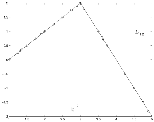
Figure 5: Direct numerical evaluation of the integral (10.6) (circles) versus the exact result (continuous straight line)

The original four-point integral (5.1) turns in this case to

$$\left\langle U_{1,2}^{4}\right\rangle_{\text{GMG}}=6\int_{\mathbf{F}}G_{\text{M}}(x,\bar{x})G_{\text{L}}(x,\bar{x})d^{2}x$$ (10.6)

where the GMM $G_{\text{M}}(x,\bar{x})=\left\langle\Phi_{1,2}(x)\Phi_{1,2}(0)\Phi_{1,2}(1)\Phi_{1,2}(\infty)\right\rangle_{\text{GMM}}$ reads explicitly

$$G_{\text{M}}(x,\bar{x})=\mathcal{F}_{1,1}(x)\mathcal{F}_{1,1}(\bar{x})-\kappa^{2}\mathcal{F}_{1,3}(x)\mathcal{F}_{1,3}(\bar{x})$$ (10.7)

where

$$\kappa^{2}=\dfrac{(1-2b^{2})^{2}\gamma(b^{2})}{\gamma^{2}(2b^{2})\gamma(2-3b^{2})}$$ (10.8)

and the conformal blocks are

$$\mathcal{F}_{1,1}(x) =x^{1-3b^{2}/2}(1-x)^{1-3b^{2}/2}{}_{2}F_{1}(2-3b^{2},1-b^{2},2-2b^{2},x)$$ (10.9)

$$\mathcal{F}_{1,3}(x) =x^{b^{2}/2}(1-x)^{b^{2}/2}{}_{2}F_{1}(-1+3b^{2},b^{2},2b^{2},x)$$

The Liouville correlation function $G_{\text{L}}(x,\bar{x})=\left\langle V_{g}(x)V_{g}(0)V_{g}(1)V_{g}(\infty)\right\rangle_{\text{L}}$ is represented in the form

$$G_{\text{L}}(x,\bar{x})=\mathcal{R}_{g}\int^{\prime}\frac{dP}{4\pi}r_{g}(P)\mathcal{F}_{P}\left(\left.\begin{array}[c]{cc}\Delta_{g}&\Delta_{g}\\ \Delta_{g}&\Delta_{g}\end{array}\right|x\right)\mathcal{F}_{P}\left(\left.\begin{array}[c]{cc}\Delta_{g}&\Delta_{g}\\ \Delta_{g}&\Delta_{g}\end{array}\right|\bar{x}\right)$$ (10.10)

where the complicated expressions for the Liouville structure constants are reduced to

$$\mathcal{R}_{g}=\left(\gamma(b^{2})b^{2-2b^{2}}\right)^{(Q-4g)/b}\frac{\Upsilon_{b}^{4}(b)\Upsilon_{b}^{4}(2g)}{\pi^{2}\Upsilon_{b}^{4}(2g-Q/2)}$$ (10.11)

and

$$r_{g}(P) =\frac{\pi^{2}\Upsilon_{b}(2iP)\Upsilon_{b}(-2iP)\Upsilon_{b}^{4}(2g-Q/2)}{\Upsilon_{b}^{2}(b)\Upsilon_{b}^{2}(2g-Q/2-iP)\Upsilon_{b}^{2}(2g-Q/2+iP)\Upsilon_{b}^{4}(Q/2-iP)}$$ (10.12)

$$=\sinh 2\pi b^{-1}P\sinh 2\pi bP\exp\left(-8\int_{0}^{\infty}\frac{dt}{t}\frac{\sin^{2}Pt\left(\cosh^{2}(Q-2g)t-e^{-Qt}\cos^{2}Pt\right)}{\sinh bt\sinh b^{-1}t}\right)$$

The general symmetric conformal block $\mathcal{F}_{P}\left(\left.\begin{array}[c]{cc}\Delta_{g}&\Delta_{g}\\ \Delta_{g}&\Delta_{g}\end{array}\right|x\right)$ is evaluated numerically through the recursive procedure introduced in ([21]) (a summary can be found in the more accessible paper [3]). As usual, the prime near the integral sign indicates possible discrete terms. In this study we consider only the region $1<b^{-2}<5$ where such extra terms don’t appear and the integral in (10.10) can be understood literally. In fig.5 the results of the numerical evaluation of the integral (10.6) are shown as circles. Notice, that near the break at $b^{-2}=3$ this integral converges very slowly near $x=0$, $1$ and $\infty$. Numbers in fig.5 in this region require proper modification of the integration algorithm. A solution to this problem, as well as other interesting details related to the numerical evaluation of (10.6) will be reported as a separate publication.

11 Comparing with martix models

It is of course very interesting to compare our expression (9.1) with the correlation numbers arising in the matrix model context. Unfortunately this is not straightforward. The standard formulations of the matrix models are interpreted mostly in terms of genuine rational minimal models with $b^{2}=p/p^{\prime}$ and involve only degenerate CFT matter fields. Moreover, the main bulk of the matrix model results contains the field theory related information in rather ciphered form. It still takes a considerable effort to disentangle the relevant correlation functions and interpret them in terms of the minimal gravity.

There is a matrix model example where the continuous interpretation is unambiguous and in addition the matter central charge varies continuously, so that our treatment of the generalized minimal gravity seems to be relevant. Recently I.Kostov [22] worked out a new exciting result about the so-called gravitational $O(n)$ model. This model is a random lattice covered by self-avoiding polymer loops, each component bringing up the weight factor $n$. The critical thermodynamics is controlled by two parameters, the “cosmological constant” $x$ coupled to the size of the lattice and the “mass” parameter $t$, which regulates the length of the polymers. Both parameters are chosen as the deviations of the corresponding absolute activities from the double critical point where the lattice size and loop length “blow up” simultaneously. The critical singularity in the neighborhood of this point is the subject of continuous field theory.

According to ref.[22] the singular part $Z(t,x)$ of the genus $0$ partition function admits the following simple description. Introduce the (standard in the $O(n)$ model) parameterization of the loop weight $-2<n<2$

$$n=-2\cos(\pi g)$$ (11.1)

in terms of the variable $1<g<2$. Also let $Z(x,t)$ be the singular part of the genus $0$ partition function and

$$u=-(g-1)Z_{xx}$$ (11.2)

its second derivative in $x$. Then $u$ is a solution to the following simple transcendental equation

$$u^{p}+tu^{p-1}=x$$ (11.3)

where $p=(g-1)^{-1}$. Equations (11.3) and (11.2) result in the following expansion

$$Z =tx^{2}+x^{g+1}\sum_{\begin{subarray}{c}n=0\\ n\neq 1\end{subarray}}^{\infty}\frac{\Gamma(g(n-1)-n-1)}{n!\Gamma(g(n-1)-2n+2)}\left(tx^{1-g}\right)^{n}$$ (11.4)

$$=x^{g+1}\left(\frac{-1}{(g-1)g(g+1)}+tx^{1-g}+\frac{\left(tx^{1-g}\right)^{2}}{2(g-3)}+\frac{\left(tx^{1-g}\right)^{3}}{6}+\frac{(g-2)\left(tx^{1-g}\right)^{4}}{8}+\ldots\right)$$

On the other hand, the critical dilute polymers on the random lattice admit the standard continuous interpretation in terms of GMG with[23]

$$c_{\text{M}}=13-6(g+g^{-1})$$ (11.5)

This is one of the occasions where the GMM $\mathcal{M}_{b^{2}}$ is relevant as the matter field theory, the parameters being related as

$$g=b^{-2}$$ (11.6)

Moreover, the GMM operator coupled to the off-critical “mass” of the polymer loop is most likely the degenerate $\Phi_{1,3}$ field and we’re dealing with the GMG perturbed by the composite field

$$U_{1,3}=\Phi_{1,3}V_{b^{-1}-b}$$ (11.7)

Notice the particular choice of the Liouville “dressing”, which turns out to be relevant in the gravity context at $1<b^{-2}<3$[23, 24]. Therefore, the coefficients in the expansion (11.4) are interpreted as the multipoint correlation functions of this field in the corresponding GMG. Since the overall normalization of the partition function depends on the scale and cannot be fixed in the universal way, it is natural to relate the normalized correlation functions

$$Z_{\text{L}}^{-1}\left\langle U_{1,3}^{n}\right\rangle_{\text{GMG}}=\frac{\Gamma(b^{-2}(n-1)-n-1)\Gamma(2-b^{-2})}{\Gamma(b^{-2}(n-1)-2n+2)\Gamma(-1-b^{-2})}(2\pi L_{\text{eg}})^{n}$$ (11.8)

The rescaling factor $L_{\text{eg}}$ is introduced here because the normalization of the dimensional cosmological constant $\mu$ is different from that of $x$ and also the field $U_{1,3}^{\text{(mat)}}$ coupled to the parameter $t$ is normalized differently from our $U_{1,3}$. The rescaling factor relates the dimensionless combinations

$$U_{1,3}^{\text{(mat)}}x^{g-1}=\left(2\pi L_{\text{eg}}\right)^{-1}U_{1,3}$$ (11.9)

It is easy to find this factor explicitly, comparing the GMG two- and three-point functions (4.9) with the corresponding terms in (11.8)[7]

$$L_{\text{eg}}=\frac{\gamma(b^{-2}-1)\left[-\gamma(b^{2})\gamma(2-3b^{2})\right]^{1/2}}{2(2-b^{-2})(\pi\mu\gamma(b^{2})^{b^{-2}-1})}$$ (11.10)

The four-point case of (11.8) reads

$$Z_{\text{L}}^{-1}\left\langle U_{1,3}^{4}\right\rangle_{\text{GMG}}=-3(g-2)(g-1)g(g+1)(2\pi L_{\text{eg}})^{4}$$ (11.11)

At the same time, our expression (9.1) gives for this case

$$\left\langle\left\langle\mathcal{U}_{1,3}^{4}\right\rangle\right\rangle=-(g+1)g(g-1)b^{-1}\Sigma_{1,3}$$ (11.12)

where

$$b^{-1}\Sigma_{1,3}=\frac{3}{2}\left(g+3-\left|g-1\right|-\left|g-3\right|-\left|g-5\right|\right)$$ (11.13)

and at $1<g<3$

$$b^{-1}\Sigma_{1,3}=3(g-2)$$ (11.14)

in agreeable consent with (11.11).

Acknowledgments

Authors are grateful to B.Feigin, I.Kostov, A.Litvinov, V.Petkova and A.Zamolodchikov for useful discussions. Our collaboration was supported by INTAS under the grant #INTAS-OPEN-03-51-3350. A.B was supported by Russian Foundation for Basic Research under the grant #RBRF 04-02-16027, by the RAS program ”Elementary particles and the fundamental nuclear physics” and the Scienific School grant 2044.2003.2. As usual, Al.Z’s creativity was mostly inspired by Galina Gritsenko. Besides that Al.Z acknowledges the hospitality and stimulating scientific atmosphere of the Theoretical Physics Laboratory at RIKEN, where the main part of the article has been written. His efforts were supported also by the European Committee under contract EUCLID HRPN-CT-2002-00325. The organizers of the LAPP conference “RAQIS 05” gave us a rare occasion to work for a while in a personal contact and coordinate in this way the final version the manuscript.

Abstract

We consider the partition function of the 2D free massive Majorana fermion coupled to the quantized metric of the spherical topology. By adding an arbitrary conformal “spectator” matter we get a control over the total matter central charge. This gives an interesting continuous family of criticalities and also enables us to make a connection with the semicalssical limit. We use the Liouville field theory as the effective description of the quantized gravity. The spherical scaling function is calculated approximately but, to our belief, to a good numerical precision in almost the whole region of the spectator parameter. Impressive comparison with the predictions of the solvable matrix model gives rise to a more general model of random lattice statistics, which is most probably not solvable by the matrix model technique but reveals a more general pattern of critical behavior. We hope that numerical simulations or series extrapolation will be able to reveal our family of scaling functions.

1 Introduction

It was demonstrated in recent developments that the Liouville field theory (LFT) is an effective tool to study relevant problems of 2D quantum gravity [1]. The field theory of two-dimensional gravity, based on LFT, is currently believed to give an effective description of the universal critical behavior in certain models of statistical physics called the random lattice spin systems. These systems were in fact first introduced rather as the models of the continuous 2D gravity itself [2, 3, 4, 5] then from the internal needs of the statistical mechanics, basic motivation coming from the Polyakov’s formulation of the string theory [6]. The random lattice models (RLM) can be thought of as the ordinary lattice systems but defined on a general graph of fixed topology, the graph itself being a dynamical degree of freedom and subject to the averaging in the partition sum. From this point of view the name “dynamical lattice” or “dynamical triangulations” [5] seems more correct then the traditional reference RLM. It has been argued long ago that such “naive” version of the Regge calculus [7] at large lattice size reveals interesting critical behavior (see e.g. [4]). Moreover, the critical exponents occur to coincide with those in the continuous description through the field theoretic path integral over all metrics on a surface [8]. It has been realized that the Liouville field theory might be a convenient instrument to treat such problems, especially in the DDK (David-Distler-Kawai) formulation [9, 10].

Further development of the field theoretic approach to the 2D gravity required essentially a better understanding of LFT as a conformal field theory. Despite some attempts based on the “analytic continuation in the number of integrations” [11, 12], the progress was slow. It was tempered probably by the superficial but persistent idea that the structures studied earlier in the rational conformal field theories (CFT) feature to some extent the general pattern of CFT. Finally, in 1992 H.Dorn and H.Otto [13] supported the belief that LFT is a solvable CFT and gave an explicit expression for the three-point correlation function. Unfortunately up to this time the topic was completely out of fashion and further development went slowly [14, 15]. This is because, with the exception of certain boundary versions [16, 17], the application of new results in the string theory remains problematic.

In this article we would like to put forward another, opposite side of LFT (and general continuous 2D gravity), its role as the effective field theory of the RLM critical behavior. Many interesting models of dynamical lattice are exactly solvable by the matrix model technique [18]. First 2D gravity applications appeared already in [2]. This gave rise to another popular idea that the matrix model patterns of critical behavior cover completely all universality classes in RLM and therefore all possible continuous 2D gravities. However we find this idea doubtful and one of the main motivations of this study is to justify this concern. To this order we study the theory of 2D massive Majorana fermion coupled to the quantized gravity. This field theory is supposed to be a continuous description of the random lattice Ising model (RLIM), as first formulated and solved by V.Kazakov [19] (for more detailed study see [20]). And indeed, the critical exponents of RLIM are known [8] to be reproduced correctly in the LFT description. Here we go beyond the critical exponents and try to evaluate a scaling function, the one related to the spherical partition function of the massive (perturbed) matter. For the time being LFT approach fails to give a comprehensive answer for such scaling functions. Instead it offers some critical correlation functions (see e.g., [11, 21, 12] or [22, 23] for more recent studies) and thus few first terms of the conformal perturbative expansion. However, in [1] it was demonstrated that even this restricted information turns out rather useful if certain conjectures are made about the analytic structure of the scaling function. In fact these conjectures, although they are not universal and some explicit counterexamples are known, seem rather natural and are justified by a number of particular examples. Under these analytic assumptions, the perturbative information can be treated through a combined analytic-numeric procedure [1] (efficiency of this procedure has been earlier observed in the case of classical gravity in [24]) and results in approximate, but sometimes impressively accurate numerical description of the scaling function.

Below we perform the same program for the Majorana fermion CFT perturbed by the mass term. The spherical scaling function obtained in this way can be compared with the exact one evaluated in the matrix model framework. In fact we consider a more general model where an additional conformal matter is added, which remains always critical but allows us an access over the LFT parameter which can now vary continuously. We propose to attribute the corresponding scaling functions to a kind of generalization of the standard RLIM, a result of the “naive” decoration of the statistical weights by a “determinant” factor. This generalized RLIM is hardly exactly solvable in general but likely can be studied numerically through the extrapolations of the finite $N$ data [25] or through the MC simulations [26, 5]. If our conjecture is correct, such studies should reveal new types of critical behavior, never seen before in the matrix model studies.

2 Massive fermion coupled to Liouville

Our model is defined through the following local Lagrangian

$$\mathcal{L}_{m}=\mathcal{L}_{\text{L}}(b)+\mathcal{L}_{\text{ising}}+\mathcal{L}_{\text{sp}}+\frac{m}{2\pi}\varepsilon e^{2a\phi}$$ (2.1)

where $\mathcal{L}_{\text{L}}$ is the usual Liouville action with cosmological coupling constant $\mu$ and parameter $b$

$$\mathcal{L}_{\text{L}}(b)=\frac{1}{4\pi}(\partial_{a}\phi)^{2}+\mu e^{2b\phi}$$ (2.2)

For what is concerned LFT, we follow the notations of [14], in particular $V_{a}$ denotes the quantum version of the exponential Liouville field $\exp(2a\phi)$, which is a Liouville primary of dimension $\Delta_{a}^{\text{(L)}}=a(Q-a)$. The Liouville central charge (as usual $Q=b^{-1}+b$)

$$c_{\text{L}}=1+6Q^{2}$$ (2.3)

Then, $\mathcal{L}_{\text{ising}}$ is the usual $c=1/2$ free field theory of the Majorana massless fermion

$$\mathcal{L}_{\text{ising}}=\frac{1}{2\pi}\left(\psi\bar{\partial}\psi+\bar{\psi}\partial\bar{\psi}\right)$$ (2.4)

This normalization corresponds to the following massless free fermion propagators

$$\left\langle\psi(z)\psi(0)\right\rangle=\frac{1}{z};\;\;\;\left\langle\bar{\psi}(\bar{z})\bar{\psi}(0)\right\rangle=\frac{1}{\bar{z}}$$ (2.5)

The energy density operator $\varepsilon=i\bar{\psi}\psi$, which plays the role of a perturbation in (2.1), has dimension $(1/2,1/2)$. It is normalized in the standard in CFT way

$$\left\langle\varepsilon(x)\varepsilon(0)\right\rangle=\frac{1}{x\bar{x}}$$ (2.6)

Finally, as in ref.[1] we added a “spectator” CFT of central charge $c_{\text{sp}}$ to have a control over the parameters of the Liouville gravity. This matter is not coupled to the perturbation term and therefore remains conformal, being in our formalism completely decoupled from the other degrees of freedom. Its presence is indicated by the term $\mathcal{L}_{\text{sp}}$ in the total Lagrangian. We call the resulting family of 2D gravity theories the gravitational Ising model (GIM).

For a semiclassical analysis the interaction term in the Lagrangian is better written as

$$\mathcal{L}_{\text{int}}=\frac{m}{2\pi}\left(\varepsilon e^{2a\phi}+\frac{m}{16a^{2}}e^{4a\phi}\right)$$ (2.7)

The second term in the brackets is the “trailing” counterterm needed to give the perturbing field definite dimension.

As usual, the following balance equations hold

$$c_{\text{sp}}+\frac{3}{2}+6Q^{2} =26$$ (2.8)

$$a(Q-a) =\frac{1}{2}$$

The first equation is recombined as

$$6Q^{2}=\frac{49}{2}-c_{\text{sp}}$$ (2.9)

This is the relation which determines the parameter $b$ of the model in terms of the central charge of the background matter. In particular the semiclassical regime $b\rightarrow 0$ is achieved when $c_{\text{bg}}\rightarrow-\infty$ and “pure Ising” case $c_{\text{bg}}=0$ corresponds to $b^{2}=3/4$.

According to the conventional wisdom (learned in fact from the matrix model experience and from the semiclassical intuition) in the second equation from the two solutions we choose the least one

$$a=\frac{Q}{2}-\sqrt{\frac{Q^{2}-2}{4}}$$ (2.10)

For the pure Ising model we have

$$a=b/3$$ (2.11)

while in the semiclassical regime

$$a=b/2-b^{3}/4+O(b^{7})$$ (2.12)

Self-consistency of LFT requires the parameter $b$ to remain real. This restricts the variation of $c_{\text{sp}}$ to the region $-\infty<c_{\text{sp}}\leq 1/2$. Inside this interval we always choose $b$ to be the smaller solution of (2.8) so that $0<b^{2}\leq 1$.

3 Partition function

The spherical (genus $0$) partition function $Z(m,\mu)$ scales as

$$Z(m,\mu)=\mu^{Q/b}G_{\text{sphere}}\left(\frac{m}{\mu^{s}}\right)$$ (3.1)

where the scaling function $G_{\text{sphere}}$ depends on the scale invariant combination of the coupling constants. The exponent $s$ is easily figured out from the scale dependence of the individual terms in (2.1)

$$s=ab^{-1}$$ (3.2)

This parameter varies from $s=1/2-b^{2}/4+\ldots$ in the semiclassical limit $b\rightarrow 0$ to $s=1-\sqrt{1/2}=0.29289\ldots$ at $b^{2}=1$. In the pure Ising model $s=1/3$.

Formal perturbative expansion in $\mathcal{L}_{\text{int}}$ gives

$$Z(m,\mu)=\sum_{n=0}^{\infty}\frac{(-m)^{n}}{(2\pi)^{n}n!}\left\langle\varepsilon^{n}\right\rangle_{\text{GIM}}$$ (3.3)

where $\left\langle...\right\rangle_{\text{GIM}}$ means non-normalized correlation functions in GIM. In the Liouville gravity such $n$-point functions are given by the integrals over the moduli of our sphere with $n-3$ punctures

$$\left\langle\varepsilon^{n}\right\rangle_{\text{GIM}}=\int\left\langle C\bar{C}(x_{1})C\bar{C}(x_{2})C\bar{C}(x_{3})\right\rangle\left\langle\varepsilon(x_{1})\ldots\varepsilon(x_{n})\right\rangle_{\text{ff}}\left\langle V_{a}(x_{1})\ldots V_{a}(x_{n})\right\rangle_{\text{L}}d^{2}x_{3}\ldots d^{2}x_{n}$$ (3.4)

where $\left\langle\ldots\right\rangle_{\text{ff}}$ and $\left\langle\ldots\right\rangle_{\text{L}}$ are the correlation functions respectively in the theory of free Majorana fermion and LFT while $C$ and $\bar{C}$ are familiar in 2D gravity and string theory gauge fixing ghosts. Expression (3.4) doesn’t need any comments for a reader familiar with the string theory, otherwise some details and explanations are placed in ref.[1]. There one can also find how to treat the case $n<3$, which does not fit in eq.(3.4) and therefore requires special consideration.

Again, a simple dimensional analysis shows that $\left\langle\varepsilon^{n}\right\rangle_{\text{GIM}}\sim\mu^{(Q-na)b}$ and therefore (3.3) is nothing but the power series for the scaling function $G_{\text{sphere}}$. Recall also that in the theory of fermions only the $\varepsilon$-correlations are non-zero with an even number of insertions $n=2k$. The expansion can be rewritten in the form

$$\frac{Z(m,\mu)}{Z(0,\mu)}=\sum_{k=0}^{\infty}\frac{a_{2k}}{(2\pi)^{2k}(2k)!}\left(\frac{m^{2}}{\mu^{2s}}\right)^{k}$$ (3.5)

with

$$a_{n}=Z_{\text{L}}^{-1}\mu^{ns}\left\langle\varepsilon^{n}\right\rangle_{\text{GIM}}$$ (3.6)

Here $Z_{\text{L}}$ denotes the Liouville partition function of the sphere $Z_{\text{L}}=\left\langle I\right\rangle_{\text{L}}$ (we imply that the fermionic correlation function are normalized in the standard way so that $\left\langle I\right\rangle_{\text{ff}}=1$).

As in [1] we find it convenient to introduce the fixed area partition function $Z_{A}(m)$

$$Z_{A}(m)=A\int_{\uparrow}Z(m,\mu)e^{\mu A}\frac{d\mu}{2\pi i}$$ (3.7)

the integration contour $\uparrow$ going along the imaginary axis of $\mu$ to the right from all singularities of the integrand. This partition function expands as follows

$$Z_{A}(m)=Z_{A}(0)\sum_{k=0}^{\infty}z_{2k}\eta^{2k}$$ (3.8)

where the coefficients $z_{n}$ are easily related to those in (3.5)

$$z_{n}=\frac{\pi^{ns}a_{n}\Gamma(-b^{-2}-1)}{(2\pi)^{n}n!\Gamma(-b^{-2}-1+ns)}$$ (3.9)

and the scaling parameter $\eta$ reads

$$\eta=m\left(\frac{A}{\pi}\right)^{s}$$ (3.10)

Due to the extra $\Gamma$ function in the denominator of (3.9) convergence of the series (3.8) is much better then that of (3.5). In fact it is absolutely convergent and defines an entire scaling function of $t=\eta^{2}$

$$z(t)=\sum_{k=0}^{\infty}z_{2k}t^{k}$$ (3.11)

4 Perturbative terms

As usual (see e.g., [13, 1]) the Liouville partition function is restored from the three-point function in LFT [13, 14]

$$Z_{\text{L}}=\left[\pi\mu\gamma(b^{2})\right]^{Q/b}\frac{1-b^{2}}{\pi^{3}Q\gamma(b^{2})\gamma(b^{-2})}$$ (4.1)

In the same way, the normalization (2.6) corresponds to the following (unnormalized) two-point function [1]

$$\left\langle\varepsilon\varepsilon\right\rangle_{\text{GIM}}=-\left(\pi\mu\gamma(b^{2})\right)^{(Q-2a)/b}\frac{\gamma(2ab-b^{2})\gamma(2ab^{-1}-b^{-2})}{\pi(Q-2a)}$$ (4.2)

For the first two coefficients in (3.11) we obtain

$$z_{0} =1$$ (4.3)

$$z_{2} =\frac{\gamma(b^{2}(2s-1))\Gamma(b^{-2}-1)\gamma^{1-2s}(b^{2})}{8\Gamma(1+b^{-2}-2s)}$$

Next perturbative coefficient $z_{4}$ requires more involved calculations. Basically it is reduced to the following integral

$$z_{4}=\frac{1}{24(2\pi)^{4}}\int\left\langle\varepsilon(x)\varepsilon(0)\varepsilon(1)\varepsilon(\infty)\right\rangle_{\text{ff}}\left\langle\left\langle V_{a}(x)V_{a}(0)V_{a}(1)V_{a}(\infty)\right\rangle\right\rangle_{\text{L}}^{(A)}d^{2}x$$ (4.4)

where the normalized fixed area Liouville correlation functions

$$\left\langle\left\langle\ldots\right\rangle\right\rangle_{\text{L}}^{(A)}=\frac{\left\langle\ldots\right\rangle_{\text{L}}^{(A)}}{Z_{\text{L}}^{(A)}}$$ (4.5)

are defined through the fixed area partition function

$$Z_{\text{L}}^{(A)}=\left(\frac{\pi\gamma(b^{2})}{A}\right)^{Q/b}\frac{\Gamma(2-b^{2})}{\pi^{3}b^{3}\gamma(b^{2})\Gamma(b^{-2})}$$ (4.6)

and the fixed area unnormalized correlations

$$\left\langle V_{a_{1}}\ldots V_{a_{n}}\right\rangle_{\text{L}}^{(A)}=A\int_{\uparrow}\left\langle V_{a_{1}}\ldots V_{a_{n}}\right\rangle_{\text{L}}e^{\mu A}\frac{d\mu}{2\pi i}=\frac{\left\langle V_{a_{1}}\ldots V_{a_{n}}\right\rangle_{\text{L}}|_{\mu\rightarrow A^{-1}}}{\Gamma(-b^{-2}-1+b^{-1}\sum_{i=1}^{n}a_{i})}$$ (4.7)

In the four-point case the Liouville correlation function can be constructed almost explicitly as the holomorphic-antiholomorphic decomposition [14]. We quote the relevant formulas explicitly below in sect.10, where the problem of the fourth-order coefficient is discussed in some more detail. Here we present only the matter four-point function $\left\langle\varepsilon(x)\varepsilon(0)\varepsilon(1)\varepsilon(\infty)\right\rangle_{\text{ff}}$ . It is made of the free fermion propagators and has a factorized form

$$\left\langle\varepsilon(x)\varepsilon(0)\varepsilon(1)\varepsilon(\infty)\right\rangle_{\text{ff}}=F_{\text{ff}}(x)F_{\text{ff}}(\bar{x})$$ (4.8)

where

$$F_{\text{ff}}(x)=\frac{1-x+x^{2}}{x(1-x)}$$ (4.9)

We postpone the analysis of the more complicated four point term and, as a preliminary step, restrict our perturbative information to what we have explicitly in eq.(4.3). At the first sight this pity information is by no means enough to make any conclusions about the whole scaling function. We will see in a moment that when supplemented with some analytic properties of the entire scaling function (which, in order, follow from natural physical arguments) and also with an additional hypothesis about the location of its zeros, a surprisingly good description of $z(t)$ can be achieved even with these restricted data.

5 Criticality and $t\rightarrow\infty$ asymptotic

If the area of the surface is very large as compared to the characteristic scale $m^{-\rho}$ of the perturbed matter, we expect the following asymptotic

$$Z_{A}(m)\sim A^{Q^{\prime}/b^{\prime}}\exp\left(-\mathcal{E}_{0}A\right)$$ (5.1)

Here $\mathcal{E}_{0}$ is the specific (per unit area) free energy of the perturbed matter interacting with the quantized gravity. We introduced also a convenient parameter

$$\rho=(2s)^{-1}$$ (5.2)

For the dimensional reasons

$$\mathcal{E}_{0}=-m^{2\rho}f_{0}$$ (5.3)

where $f_{0}$ is some numerical constant, which depends in our model on the Liouville parameter $b^{2}$. As for the power correction $A^{Q^{\prime}/b^{\prime}}$, it can figured out through the following speculation. It is almost obvious that in our model the massive fermion develops a final correlation length $\sim m^{-\rho}$ and therefore, at the asymptotic scales we are interested in, it doesn’t influence the dynamics contributing only to the local quantities like $\mathcal{E}_{0}$. Thus, the large scale fluctuations of the surface are governed by the residual spectator matter (and the ghosts) and therefore the effective infrared Liouville theory is characterized by another parameters $b^{\prime}$ and $Q^{\prime}=1/b^{\prime}+b^{\prime}$. The latter can be found from the IR central charge balance [1]

$$1+6(Q^{\prime})^{2}+c_{\text{sp}}=26$$ (5.4)

or

$$Q^{\prime}=\sqrt{Q^{2}+\frac{1}{12}}$$ (5.5)

On all these physical accounts we assume the following $t\rightarrow\infty$ asymptotic of the scaling function $z(t)$

$$z(t)\sim\exp\left(\pi f_{0}t^{\rho}+\rho\left(Q/b-Q^{\prime}/b^{\prime}\right)\log t+O(1)\right)$$ (5.6)

Note that as usual $\mu_{\text{c}}=m^{2\rho}f_{0}$ is interpreted as the position of the critical singularity in the “grand” partition function (3.1). In other words, the critical value of $m$ is $m_{\text{c}}=\left(\mu/f_{0}\right)^{s}$.

6 Basic conjecture

Our basic conjecture states that in the region of interest $0\leq b^{2}\leq 1$ the scaling function $z(t)$ always enjoys the asymptotic (5.6) in the whole complex plane except for the negative part of the real axis, where all its zeros are located. This is very restrictive requirement for an entire function and it is this property, together with some numerical fortuity, which makes even very restricted perturbative input miraculously efficient.

At $t\rightarrow-\infty$ the asymptotic of $z(t)$ is a result of competition of two terms

$$z(t) =\exp\left(\pi f_{0}t^{\rho}e^{i\pi\rho}-\left(1/2+\delta\right)\log e^{i\pi}t+\ldots\right)+\text{c.c.}$$ (6.1)

$$=2\exp\left(\pi f_{0}(-t)^{\rho}\cos\pi\rho-\left(1/2+\delta\right)\log(-t)\right)\cos\left(\pi f_{0}(-t)^{\rho}\sin\pi\rho-\pi\left(1/2+\delta\right)\right)$$

where for convenience we have denoted

$$\rho\left(Q/b-Q^{\prime}/b^{\prime}\right)=-\frac{1}{2}-\delta$$ (6.2)

Asymptotic position of $n$-th zero $t_{n}$, $n=1,2,\ldots$ at $n\rightarrow\infty$ follows

$$-t_{n}=\left(\frac{n+\delta}{-f_{0}\sin\pi\rho}\right)^{2s}$$ (6.3)

If the zeros of an entire function are known we have (see below about the convergence problem)

$$z(t)=\prod_{n=1}^{\infty}\left(1-\frac{t}{t_{n}}\right)$$ (6.4)

and therefore

$$\log z(t)=\sum_{n=1}^{\infty}\log\left(1-\frac{t}{t_{n}}\right)=t\sum_{n=1}^{\infty}\frac{1}{-t_{n}}-\frac{t^{2}}{2}\sum_{n=1}^{\infty}\frac{1}{(-t_{n})^{2}}-\ldots$$ (6.5)

From the first two terms we find

$$z_{2}=\sum_{n=1}^{\infty}\frac{1}{-t_{n}}$$ (6.6)

and

$$z_{4}-\frac{z_{2}^{2}}{2}=r_{2}=-\frac{1}{2}\sum_{n=1}^{\infty}\frac{1}{(-t_{n})^{2}}$$ (6.7)

In our particular case the product (6.4), as well as the sum (6.6), are divergent since the order $\rho$ of our function is always $1\leq\rho<(2-\sqrt{2})^{-1}=1.70711\ldots$. It can be shown, however (see Appendix), that the sum rule (6.6) remains valid if the right hand side is understood in terms of the zeta function of the zeros $t_{n}$. A mathematically correct canonical product for the function of order $\rho<2$ with zeros at $t_{n}$ reads

$$z(t)=\exp\left(z_{2}t\right)\prod_{n=1}^{\infty}\left(1-\frac{t}{t_{n}}\right)\exp\left(\frac{t}{t_{n}}\right)$$ (6.8)

7 Numerics and approximations

$b^{2}$	$s$	$z_{2}$	$\delta$	$-f_{0}$	$-f_{0}^{\text{(exact)}}$	$z_{4}^{\text{(est)}}$	$z_{4}$
$0.05$	$0.488$	$-5.26967$	$-0.414$	$1.61954$		$13.8494$
$0.10$	$0.475$	$-2.7913$	$-0.411$	$0.831718$		$3.85341$
$0.15$	$0.463$	$-1.9818$	$-0.408$	$0.575331$		$1.91275$
$0.20$	$0.450$	$-1.59146$	$-0.404$	$0.452694$		$1.20427$
$0.25$	$0.438$	$-1.37065$	$-0.399$	$0.384486$		$0.863088$
$0.30$	$0.427$	$-1.23648$	$-0.393$	$0.344516$		$0.670052$
$0.35$	$0.415$	$-1.15384$	$-0.386$	$0.321859$		$0.547863$
$0.40$	$0.404$	$-1.10562$	$-0.378$	$0.311425$		$0.462962$
$0.45$	$0.393$	$-1.08291$	$-0.368$	$0.310866$		$0.398285$
$0.50$	$0.382$	$-1.08110$	$-0.357$	$0.319416$		$0.343762$
$0.55$	$0.372$	$-1.09830$	$-0.343$	$0.337485$		$0.292372$
$0.60$	$0.362$	$-1.13467$	$-0.327$	$0.366663$		$0.2381$
$0.65$	$0.352$	$-1.19248$	$-0.306$	$0.41011$		$0.174833$
$0.70$	$0.342$	$-1.27680$	$-0.281$	$0.473557$		$0.094298$
$0.75$	$0.333$	$-1.39733$	$-0.25$	$0.567684$	$0.563124$	$-0.016269$	$0$
$0.80$	$0.325$	$-1.57298$	$-0.21$	$0.714273$		$-0.18167$
$0.85$	$0.316$	$-1.84474$	$-0.16$	$0.964987$		$-0.462053$
$0.90$	$0.308$	$-2.32185$	$-0.10$	$1.47712$		$-1.05291$
$0.95$	$0.300$	$-3.45523$	$-0.023$	$3.04496$		$-3.04188$
$0.99$	$0.294$	$-8.75236$	$0.049$	$15.7725$		$-23.4948$

Table 1: First order approximation for $f_{0}$ at different values of $b^{2}$. We present also our analytic estimate for the forth-order perturbative coefficient $z_{4}$ through eq.(7.5)

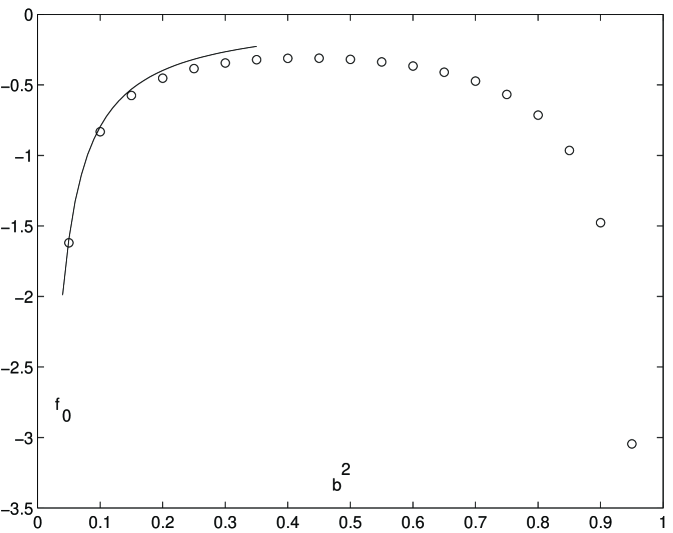
Figure 1: First order approximation for $f_{0}$ at different values of $b^{2}$ (circles). Semiclassical limit is drawn as a continuous curve.

Suppose that the asymptotic (6.3) gives a reasonably good approximation for $t_{n}$ even at small $n$. Then the sum rule (6.6) allows to relate approximately the parameter $f_{0}$ in the asymptotic (6.3) to the first perturbative coefficient $z_{2}$

$$z_{2}=\left(f_{0}\sin\pi\rho\right)^{2s}\sum_{n=1}^{\infty}\frac{1}{\left(n+\delta\right)^{2s}}=\left(f_{0}\sin\pi\rho\right)^{2s}\zeta(2s,\delta+1)$$ (7.1)

The divergent sum is evaluated as the analytic continuation through the ordinary Riemann $\zeta$-function. The first estimate for $f_{0}$ is then

$$f_{0}=-\frac{1}{\sin\pi\rho}\left(\frac{z_{2}}{\zeta(2s,\delta+1)}\right)^{\rho}$$ (7.2)

For different values of the spectator parameter $b^{2}$ these estimates are presented in Table 1 and plotted in fig.1. Two examinations allow us to evaluate the accuracy of the approximation. First is the exactly solvable point $b^{2}=3/4$ which corresponds to pure Ising (no spectator matter) and is believed to be related to a matrix model solution. Accidentally or not, the comparison of the exact matrix model result (see sect. 9 below) with our prediction for this point is impressive (table 1). Another one is the classical region $b^{2}\rightarrow 0$. Here we are dealing with the rigid sphere with the quantum gravity effects suppressed. The specific vacuum energy of the free massive fermion of mass $m$ in the flat classical background is

$$\mathcal{E}_{0}=\frac{m^{2}}{4\pi}\log m$$ (7.3)

From the scaling (5.3) and (2.12) we interpret this as the following leading behavior of $f_{0}(b^{2})$ at $b^{2}\rightarrow 0$

$$f_{0}=-\frac{1}{4\pi b^{2}}+O(1)$$ (7.4)

This asymptotic is also plotted in fig.1. Further semiclassical corrections to the vacuum energy also can be evaluated systematically in the field theory framework. The authors plan to address this interesting topic elsewhere.

The second sum rule (6.7) allows to obtain an estimate for the next perturbative coefficient $z_{4}$

$$z_{4}\approx z_{4}^{\text{(est)}}=\frac{z_{2}^{2}}{2}-\frac{1}{2}\left(-f_{0}\sin\pi\rho\right)^{4s}\zeta(4s,\delta+1)$$ (7.5)

These numbers for $z_{4}^{\text{(est)}}$ are also presented in the Table. In principle they can be compared with the direct evaluation of the integral in (4.4). This would be a crucial examination for our basic conjecture and also an estimate of the convergence of the analytic-numeric procedure. Unfortunately this direct calculation is more difficult technically. A preliminary discussion will be given in sect.10.

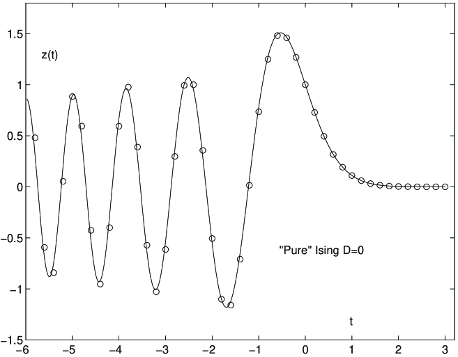
Figure 2: Scaling function $z(t)$ at the solvable point $b^{2}=0.75$. Our approximation (7.6) (circles) is compared with the exact matrix model function (8.32) (continuous curve).

Once the parameter $f_{0}$ is estimated the zeros $t_{n}$ are evaluated through the asymptotic formula (6.3). The approximate scaling function $z(t)$ is then constructed as the product (6.8). Even better convergent expression, more suitable for the numerics, is

$$z_{\text{est}}(t)=\exp\left(z_{2}t+\left(z_{4}^{\text{(est)}}-z_{2}^{2}/2\right)t^{2}\right)\prod_{n=1}^{\infty}\left(1-\frac{t}{t_{n}}\right)\exp\left(\frac{t}{t_{n}}+\frac{t^{2}}{2t_{n}^{2}}\right)$$ (7.6)

For the “pure Ising” case $b^{2}=0.75$ this scaling function is plotted in fig.2 and compared with the exact scaling function available from the matrix model solution (see below).

8 Random lattice Ising model

Now we consider a model of discrete (random lattice) gravity which seems to be directly related (in its continuous limit) to the field theory of the previous sections. Although the continuous limit is not supposed to depend essentially on the details of the microscopic lattice description, here we’ll formulate a very particular system, the Ising model on the triangular random lattice. This is basically the standard random lattice Ising system as e.g., considered in refs.[19, 20]. In this standard formulation the model is exactly solvable by the matrix model technique, and we’re going to use the essence of this solution in what follows. However, in order to match the more general pattern introduced in sect.2 with the spectator conformal matter (and in fact in order to make the situation less vulgar) we decorate this model by a $D$-component massless boson, or, in the string theory language, by immersing the system to $D$-dimensional target space. We expect that in the continuous limit this additional lattice boson simulates our “spectator matter”, at least for the spherical topology, with $c_{\text{sp}}=D$.

Take an irregular planar lattice (called also a graph or a triangulation) constructed from $N$ triangles. Planar means here that the graph can be drawn on a sphere without intersections. An example is given in fig.3. Let $\{G_{N}\}$ be the ensemble of such topologically different graphs. Let’s also enumerate the triangles of a particular graph by index $i=1,\ldots,N$ and attach to each one a spin variable $\sigma_{i}=\pm 1$. Finally, let $I_{ij}$ be the incidence matrix of the corresponding triangulation

Figure 3: A sample element of $\left\{G_{N}\right\}$ for $N=24$. Ising spins $\sigma_{i}$ are attached to the faces of the triangulation.

$$I_{ij}=\genfrac{\{}{.}{0.0pt}{}{1\;\;\text{ if triangles }i\;\text{and }j\text{ have common edge}}{0\;\;\text{otherwise\ }}$$ (8.1)

The familiar Ising model corresponds to the spin configurations distributed with the Gibbs weights $W[\left\{\sigma_{i}\right\}]=\exp\left(-\mathcal{H}[\left\{\sigma_{i}\right\}]\right)$ where

$$\mathcal{H}[\left\{\sigma_{i}\right\}]=K\sum_{i,j}I_{ij}\sigma_{i}\sigma_{j}+H\sum_{i}\sigma_{i}$$ (8.2)

and $K$ and $H$ are standard “temperature” and “magnetic field” parameters. Although a non-vanishing magnetic field makes the physics of the model much more rich and interesting, to avoid additional complications presently we restrict ourselves by the zero magnetic field $H=0$. Thermodynamic information is encoded in the microcanonic partition sum

$$Z_{N}(K)=N\sum_{{}^{\left\{G_{N}\right\}}}\det\nolimits^{-D/2}\left(\Delta_{ij}^{\text{lat}}\right)\sum_{\left\{\sigma_{i}\right\}}\exp\left(-\mathcal{H}[\left\{\sigma_{i}\right\}]\right)$$ (8.3)

Notice unusual factor of $N$ in the definition of the partition sum, which is introduced to facilitate the subsequent comparisons with the continuous theory. The determinant factor represents the discrete version of the Laplace operator

$$\Delta_{ij}^{\text{lat}}=\left(I_{ij}-3\delta_{ij}\right)^{\prime}$$ (8.4)

and introduces new “spectator central charge” parameter $D$. This discrete operator always have zero eigenvalue, which should be projected out in the definition (8.3), the prime in the last formula indicating this zero mode prescription.

As it is, the problem (8.3) does not seem easier then the continuous path integral over $g_{ab}$. To simulate a continuous surface one should take a kind of thermodynamic limit, where the size of the graph $N$ goes to infinity. In this limit direct calculation of the partition sum seems a complicated problem. Fortunately, for certain choices of statistical weights, there is a powerful machinery, which permits to calculate effectively the thermodynamic limit of the sums like (8.3). This is famous matrix model technique. Here we do not go into any details of this interesting theory, referring for example to the review [27]. We’d only like to mention that a particular case of (8.3) with $D=0$ (pure RLIM) is solved exactly in [19] and [20] (see also [29] where precisely our model of random triangulations with $D=0$ is treated). Some important things can be learned from this exact solution. We consider the asymptotic of large $N$ which only can be related to a continuous theory.

1. At generic values of the temperature parameter $K$ the $N\rightarrow\infty$ asymptotic has the form

$$Z_{N}(K)\sim\mathcal{Z}(K)N^{-5/2}e^{-E(K)N}$$ (8.5)

Here $E(K)$ is the specific (per a triangle) free energy. This function is non-universal and depends on the details of the random lattice model. For our very particular realization it can be found explicitly in [29]. On the contrary, the power-like pre-exponential dependence $N^{-5/2}$ is universal, the index $-5/2$ is known as the “pure gravity” critical exponent.

2. A criticality, like in the standard Ising model, occurs at certain value $K=K_{\text{c}}$ (the critical temperature). This value again depends on the microscopic details of the model. Our particular triangular system has [29]

$$K_{\text{c}}=\frac{1}{2}\log\frac{23}{108}$$ (8.6)

The asymptotic (8.5) changes here to

$$\,Z_{N}(K_{\text{c}})\sim\mathcal{Z}_{\text{c}}N^{-7/3}e^{-E(K_{\text{c}})N}$$ (8.7)

The power pre-exponential behavior is changed, the exponent $-7/3$ being familiar as the “gravitational Ising” critical index. In particular this change of the asymptotic means that $\mathcal{Z}(K)$ is singular at $K=K_{\text{c}}$ and in any case $\mathcal{Z}_{\text{c}}\neq\mathcal{Z}(K_{\text{c}})$.

3. The crossover scaling behavior at $K$ near the critical point is expected to be universal and a subject of the field theory application. Let

$$\tau=\frac{K-K_{\text{c}}}{K_{\text{c}}}$$ (8.8)

and $\left|\tau\right|\ll 1$. In this region it turns out relevant to introduce the “correlation size” $N_{\text{c}}$ of the lattice. While generically $N_{\text{c}}\sim 1$, near the critical point $N_{\text{c}}$ diverges. Exact solution of the RLIM shows that

$$N_{\text{c}}\sim\frac{L_{0}}{\left|\tau\right|^{3}}\gg 1$$ (8.9)

where $L_{0}$ is some (non-universal) constant dependent on the choice of the scale. In the large $N$ asymptotic of the partition function $Z_{N}(K)$ we have to distinguish the following regions:

i) At $1\ll N\ll N_{\text{c}}$ the “Ising” behavior (8.7) is observed.

ii) At $N\gg N_{\text{c}}$ the Ising spins correlate locally, contributing only to $E(K)$. The “pure gravity” asymptotic (8.5) appears with certain singular in $\tau$ contribution to $E(K)=E_{\text{reg}}(K)+E_{\text{sing}}(\tau)$, the singularity being caused by the long range (as compared to the lattice scale) correlation of the Ising spins

$$\,Z_{N}(K)\sim\mathcal{Z}(K_{\text{c}})N^{-5/2}e^{-E_{\text{reg}}(K)N-E_{\text{sing}}(\tau)N}$$ (8.10)

The singular contribution $E_{\text{sing}}(\tau)$ in the exactly solvable RLIM reads

$$E_{\text{sing}}(\tau)=e_{0}\left|\tau\right|^{3}$$ (8.11)

where the amplitude of critical singularity $e_{0}$ again depends on the choice of the scale.

iii) Crossover scaling function $F_{\text{sphere}}(y)$ appears at $N\sim N_{\text{c}}$

$$Z_{N}(K)\sim F_{\text{sphere}}\left(\frac{N}{N_{\text{c}}}\right)N^{-7/3}e^{-E_{\text{reg}}(K)N}$$ (8.12)

This function has the following asymptotic properties at small and large values of its argument

$$F_{\text{sphere}}(y) \sim\mathcal{Z}_{\text{c}}\;\;\;\;\;\;\;\;\;\;\;\;\;\;\;\;\;\;\;\;\;\;\;\;\;\;\;\;\;\;\;\;\;\;\text{at}\;\;\;y\ll 1$$ (8.13)

$$F_{\text{sphere}}(y) \sim F_{\infty}y^{-1/6}\exp\left(-L_{0}e_{0}y\right)\;\;\;\text{at\ \ \ \ }y\gg 1$$

where apparently

$$F_{\infty}=\mathcal{Z}(K_{\text{c}})N_{\text{c}}^{-1/6}$$ (8.14)

Moreover, the exact solution of the matrix model gives the scaling function $F_{\text{scaling}}(y)$ of RLIM in explicit form. Before discussing it, let us conjecture natural generalizations of the above scaling relations for model (8.3) with $-\infty<D\leq 1/2$, which we find natural to name the generalized random lattice Ising model (GRLIM). First, the assumed relation to the continuous quantum gravity described in sect.2 suggests to replace the generic asymptotic (8.5) by

$$Z_{N}(K,D)\sim\mathcal{Z}(K,D)N^{-d_{\text{g}}(D)}e^{-E(K,D)N}$$ (8.15)

where the familiar $c_{\text{sp}}=D$ KPZ [8] scaling is expected

$$d_{\text{g}}(D)=\frac{1}{12}\left(25-D+\sqrt{\left(25-D\right)\left(1-D\right)}\right)$$ (8.16)

A critical point $K=K_{\text{c}}(D)$ is expected to exist in general, where the asymptotic is different

$$Z_{N}(K_{\text{c}},D)\sim\mathcal{Z}_{\text{c}}(D)N^{-d_{\text{c}}(D)}e^{-E(K_{\text{c}},D)N}$$ (8.17)

Now

$$d_{\text{c}}(D)=\frac{1}{24}\left(49-2D+\sqrt{\left(49-2D\right)\left(1-2D\right)}\right)$$ (8.18)

Again $E(K,D)$ is interpreted as the specific (per triangle) free energy of the infinite system, which develops a singularity at $K=K_{\text{c}}$

$$E(K,D)=E_{\text{reg}}(K,D)+e_{0}(D)\left|\tau\right|^{2\rho(D)}$$ (8.19)

where

$$\rho(D)=\frac{\left(\sqrt{49-2D}-\sqrt{1-2D}\right)\left(\sqrt{49-2D}+\sqrt{25-2D}\right)}{48}$$ (8.20)

$\tau$ is defined in eq.(8.8) and $e_{0}(D)$ is the amplitude of critical singularity. Finally, in the scaling region $\left|\tau\right|\ll 1$ the correlation size scales as

$$N_{\text{c}}(D)\sim L_{0}(D)\left|\tau\right|^{-2\rho(D)}$$ (8.21)

and becomes large as compared to the lattice scales. In this region and at $N\sim N_{\text{c}}$ equation (8.12) is generalized to

$$Z_{N}(K,D)\sim F_{\text{sphere}}\left(\frac{N}{N_{\text{c}}},D\right)N^{-d_{\text{c}}(D)}e^{-E_{\text{reg}}(K,D)N}$$ (8.22)

where the scaling function now depends on $D$ and

$$F_{\text{sphere}}(y) \sim\mathcal{Z}_{\text{c}}(D)\;\;\;\;\;\;\;\;\;\;\;\;\;\;\;\;\;\;\;\;\;\;\;\;\;\;\;\;\;\;\;\;\;\;\;\;\;\;\;\;\;\;\;\;\;\;\;\;\text{at}\;\;\;y\ll 1$$ (8.23)

$$F_{\text{sphere}}(y) \sim F_{\infty}y^{d_{\text{c}}(D)-d_{\text{g}}(D)}\exp\left(-e_{0}(D)L_{0}(D)y\right)\;\;\;\text{at\ \ \ \ }y\gg 1$$

Notice, that we expect certain symmetry $\tau\rightarrow-\tau$ of the singular part. This can be argued form the Ising model duality. This symmetry holds also over a random lattice, mapping the model on a triangulation on a similar model on a $\phi^{3}$ graph. Of course these arguments rely strongly on the universality of the critical behavior and support only the symmetry of the scale independent characteristics. For example, the scale-dependent factors like $L_{0}(D)$, $e_{0}(D)$ as well as the overall normalization of the scaling function, can well be different in the low and high temperature phases $\tau>0$ and $\tau<0$ respectively. We didn’t make this fact explicit above to render the equations more transparent.

It is easy to relate all these scaling characteristics to the observables of the field theory problem discussed in sect.2. Of course the Liouville parameters $b$ and $a$ in (2.1) are

$$b =\sqrt{\frac{49-2D}{48}}-\sqrt{\frac{1-2D}{48}}$$ (8.24)

$$a =\sqrt{\frac{49-2D}{48}}-\sqrt{\frac{25-2D}{48}}$$

The scaling function $z(t)$ defined in eq.(3.11) is, up to the overall normalization and the normalization of the argument, nothing but $F_{\text{sphere}}(y,D)$ in GRLIM. More precisely

$$f_{\text{sphere}}(y,D)=\frac{F_{\text{sphere}}(y,D)}{F_{\text{sphere}}(0,D)}=z(t)$$ (8.25)

where $y\sim t^{\rho}$ while the coefficient depends on the choice of the scale (or precise definition of $N_{\text{c}}$). To be slightly more explicit, let us introduce dimensional parameters $a_{0}$ and $m_{0}$ which relate the area $A$ and the coupling constant $m$ as defined in sect.2 to $N$ and $\tau$ of the microscopic model

$$A =a_{0}N$$ (8.26)

$$m =m_{0}\tau$$

Let us also fix unambiguously the correlation size of the surface by the relation

$$A_{\text{c}}=\pi m^{-2\rho}$$ (8.27)

so that

$$y=\frac{A}{A_{\text{c}}}=t^{\rho}$$ (8.28)

and

$$L_{0}=\frac{\pi}{a_{0}m_{0}^{2\rho}}$$ (8.29)

In particular, the amplitude $e_{0}(D)$ in eq.(8.19) is related to the universal parameter $f_{0}$ of eq.(5.3)

$$L_{0}(D)e_{0}(D)=\pi f_{0}$$ (8.30)

Once the normalization is fixed we can compare the normalized GRLIM scaling function $f_{\text{sphere}}(y,D)$ with our perturbative prediction (3.11), (4.3)

$$f_{\text{sphere}}(y,D)=1+z_{2}y^{2s}+z_{4}y^{4s}+\ldots$$ (8.31)

as well as with the asymptotic, controlled mainly by the parameter $f_{0}$ from table 1. In particular, in the exactly solvable case $D=0$ this scaling function is extracted explicitly from the matrix model treatment (see next section for more details)

$$f_{\text{sphere}}(y,0)=3^{2/3}\Gamma\left(\frac{2}{3}\right)\operatorname*{Ai}\left(\frac{3^{2/3}l_{\text{eg}}^{2}}{4}y^{2/3}\right)$$ (8.32)

This is the function plotted in the continuous line in fig.2. In (8.32) $l_{\text{eg}}$ is a numeric constant

$$l_{\text{eg}}=2\gamma(1/3)\gamma^{2/3}(3/4)=1.919868134043972\ldots$$ (8.33)

caused by our particular definition of $N_{\text{c}}$ and $\operatorname*{Ai}(x)$ is the Airy function

$$\text{ }\operatorname*{Ai}(x)=\frac{1}{3^{2/3}}\sum_{n=0}^{\infty}\frac{\left(-3^{1/3}x\right)^{n}}{n!\Gamma(2/3-n/3)}$$ (8.34)

Notice that according to this power expansion of the Airy function, $z_{4}=0$ at the pure Ising point $b^{2}=0.75$. In the last section of this paper we are going to support this conclusion from the point of view of the Liouville gravity integral (4.4).

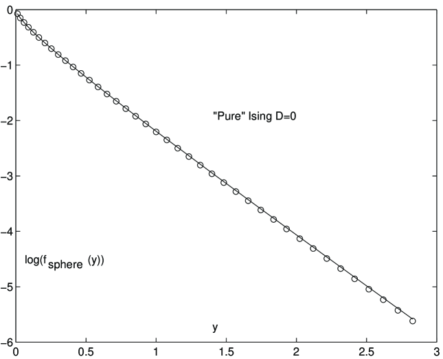
Figure 4: Logarithmic plot of $f_{\text{sphere}}(y)$ for the “pure Ising” model $D=0$. Circles – our approximation, continuous – exact matrix model function.

The essence of the exact solution to the matrix model in the continuous limit will be discussed in the next section. What we would like to stress here, is that the generalized random lattice model at generic $D\leq 1/2$ is still an interesting model of the dynamical lattice statistics. Although our field theoretic approach involves many poorly justified conjectures and assumptions, it provides very definite predictions for measurable observables in GRLIM, equally well at $D=0$ and $D\neq 0$, where the famous matrix models (sometimes traded as a substitute for the field theory) fail to answer any questions. Numerical coincidence or not, our data presented in fig.2 give astonishingly good and detailed description of the exact matrix model scaling function. Fig.4 presents similar comparison for $f_{\text{sphere}}(y,0)$ for physically relevant positive $t$ and for much larger values of $y$ where the exponential asymptotic (5.1) is clearly seen. Notice that this plot (in the logarithmic scale) follows the falloff of $f_{\text{sphere}}(y,0)$ in at least $3$ orders of magnitude. In fig.5 we also present our prediction for the scaling function $f_{\text{sphere}}(y,D)$ for $D=-2$ ($b^{2}=0.530049\ldots$) and $D=-20$ ($b^{2}=0.191377\ldots$).

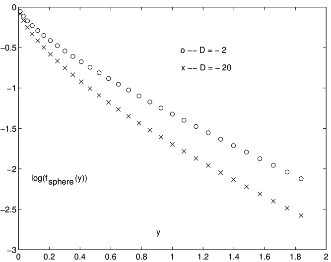
Figure 5: Our approximation for the scaling functions $f_{\text{sphere}}(y,D)$ at $D=-2$ and $D=-20$.

9 Minimal gravity point (pure Ising)

This point corresponds to $b^{2}=3/4$ (or, in the spectator matter language, to $c_{\text{sp}}=D=0$). The situation is supposed to be described by the two matrix model by Kazakov [19, 20]. In the double scaling limit of this matrix model the genus $0$ partition function $Z(T,x)$ is determined through

$$u(T,x)=Z_{xx}(T,x)$$ (9.1)

where $u(T,x)$ is the solution to the following (renormalized) algebraic equation [19]

$$x=u^{3}-\frac{3}{4}T^{2}u$$ (9.2)

Here $x$ is interpreted as the cosmological constant while $T$ corresponds to the off-critical temperature of the Ising system. Precise relation between the parameters $T$ and $x$ in this section and, respectively, $\tau$ and the activity conjugated to $N$ in the previous one, depends on the microscopic realization of the RLIM. In the particular formulation given in sect.8 these parameters can be related using the explicit expressions of [29].

From (9.1) and (9.2) the expansion in $T^{2}$ follows

$$Z(T,x) =-\frac{x^{7/3}}{3}\sum\frac{\Gamma(2n/3-7/3)}{n!\Gamma(2/3-n/3)}\left(-\frac{3T^{2}}{4x^{2/3}}\right)^{n}$$ (9.3)

$$=\frac{9x^{7/3}}{28}+\frac{9T^{2}x^{5/3}}{40}+\frac{3T^{6}x^{1/3}}{128}+\frac{3T^{8}}{1024x^{1/3}}+\ldots$$

The fixed area $a$ partition function (we introduce new letter $a$ for this area instead of $A$, because the normalization of the conjugated cosmological constant $x$ differs from that of $\mu$)

$$Z_{a}(T)=a\int_{\uparrow}Z(T,x)e^{ax}\frac{dx}{2\pi i}$$ (9.4)

where the contour $\uparrow$ is as in (3.7). This is transformed to

$$Z_{a}(T)=-\frac{1}{3}a^{-7/3}\int_{\uparrow}\exp\left(v^{2}-\frac{3}{4}a^{2/3}T^{2}v^{2/3}\right)\frac{dv}{\pi iv^{1/3}}$$ (9.5)

and then expressed in terms of the Airy function

$$Z_{a}(T)=-\frac{a^{-7/3}}{3^{1/3}}\operatorname*{Ai}\left(\frac{(3a)^{2/3}T^{2}}{4}\right)$$ (9.6)

The relation between the scales

$$Ta^{1/3}=l_{\text{eg}}m\left(\frac{A}{\pi}\right)^{1/3}$$ (9.7)

($l_{\text{eg}}$ is from eq.(8.33)) is easily recovered comparing the $T^{2}$ order of (9.3) with $z_{2}$ of (4.3). Finally (9.6) is reduced to

$$Z_{a}(T)=-3^{-1/3}A^{-7/3}\operatorname*{Ai}\left(\left(m\left(3A/\pi\right)^{1/3}l_{\text{eg}}/2\right)^{2}\right)$$ (9.8)

Up to normalization this is equivalent to (8.32). In particular

$$Z_{a}\sim\exp\left(-l_{\text{eg}}^{3}m^{3}\frac{A}{4\pi}\right)$$ (9.9)

From this asymptotic we get

$$-f_{0}^{\text{(exact)}}=\frac{l_{\text{eg}}^{3}}{4\pi}=\frac{2\gamma^{3}(1/3)}{\pi\gamma^{2}(1/4)}=0.563124\ldots$$ (9.10)

the number quoted in table 1.

10 Four-point integral

Here we consider on a preliminary footing the problem of the forth order correction (4.4). The matter ingredient of the integrand is quite simple, see eq.(4.8). An explicit representation of the Liouville four-point function can be taken from [14]. Here we need only the “symmetric” case of this function with all four external dimensions equal (and in fact equal to $1/2$). For numerical purposes it is convenient to reduce the holomorphic-antiholomorphic (spectral) integral to the form [1]

$$\left\langle V_{a}(x)V_{a}(0)V_{a}(1)V_{a}(\infty)\right\rangle_{\text{L}}^{(A)} =\mathcal{R}_{a}^{(A)}\times$$ (10.1)

$$\int^{\prime}\frac{dP}{4\pi}r_{a}(P)\mathcal{F}_{P}\left(\left.\begin{array}[c]{cc}1/2&1/2\\ 1/2&1/2\end{array}\right|x\right)\mathcal{F}_{P}\left(\left.\begin{array}[c]{cc}1/2&1/2\\ 1/2&1/2\end{array}\right|\bar{x}\right)$$ (10.6)

where the overall factor is

$$\mathcal{R}_{a}^{(A)}=\frac{\left(\pi\gamma(b^{2})b^{2-2b^{2}}A^{-1}\right)^{(Q-4a)/b}}{\pi^{2}\Gamma(-b^{-2}-1+4b^{-1}a)}\frac{\Upsilon_{b}^{4}(b)\Upsilon_{b}^{4}(2a)}{\Upsilon_{b}^{4}(2a-Q/2)}$$ (10.7)

The weight function

$$r_{a}(P)=\frac{\pi^{2}\Upsilon_{b}(2iP)\Upsilon_{b}(-2iP)\Upsilon_{b}^{4}(2a-Q/2)}{\Upsilon_{b}^{2}(b)\Upsilon_{b}^{2}(2a-Q/2-iP)\Upsilon_{b}^{2}(2a-Q/2+iP)\Upsilon_{b}^{2}(Q/2-iP)\Upsilon_{b}^{2}(Q/2+iP)}$$ (10.8)

admits the following convenient integral representation

$$r_{a}(P) =\sinh 2\pi b^{-1}P\sinh 2\pi bP\times$$ (10.9)

$$\exp\left(-8\int_{0}^{\infty}\frac{dt}{t}\frac{\sin^{2}Pt\left(\cosh^{2}(Q-2a)t-e^{-Qt}\cos^{2}Pt\right)}{\sinh bt\sinh b^{-1}t}\right)$$

The prime near the integral sign in (10.1) indicates possible discrete terms. The general block function

$$\mathcal{F}_{P}\left(\left.\begin{array}[c]{cc}\Delta_{1}&\Delta_{3}\\ \Delta_{2}&\Delta_{4}\end{array}\right|x\right)=\raisebox{-33.93831pt}{\includegraphics[height=75.12502pt,width=164.00247pt]{lblock.eps}}$$ (10.10)

is effectively computable through the recursive relation of [28]. In our problem we are interested in the particular case $\Delta_{1}=\Delta_{2}=\Delta_{3}=\Delta_{4}=1/2$ but general $P$.

It is easy to see that in our example of free fermion at least one discrete term is always present in the r.h.s of (10.1). It is located at $iP=\pm(Q/2-2a)$. Moreover, if $b^{2}<b_{1}^{2}$, where $b_{1}^{2}=\left(\sqrt{8/3}+1\right)^{-1}\approx 0.38$, a second discrete term appears at $iP=\pm(Q/2-2a-b)$, and so on. For the values of $b^{2}$ below $b_{1}^{2}$ there are more discrete terms and in the classical limit only these terms count. All these complications temper the straightforward numerical analysis of the integral (4.4). The problem will be studied in more details in a separate publication.

In the “matrix model” case $b^{2}=0.75$ the situation is essentially simplified. First, it is easy to see that the discrete term is singular near this point. Here $4a=Q-b$ and we are at the first order resonance. However, in the fixed area correlation function (4.7) this pole is canceled out by the $\Gamma$-function in the denominator and we are left with a finite expression. Moreover, this denominator kills completely the residual integral part and the only remaining contribution is the discrete term. In this case it is not difficult to evaluate explicitly the fixed area Liouville four-point function (see e.g., [1])

$$\left\langle V_{a}(x)V_{a}(0)V_{a}(1)V_{a}(\infty)\right\rangle_{\text{L}}^{(A)}=\frac{4\left[K(x)K(1-\bar{x})+K(\bar{x})K(1-x)\right]}{b\left[x\bar{x}(1-x)(1-\bar{x})\right]^{1/6}}$$ (10.11)

where

$$K(x)=\frac{1}{2}\int\left[t(1-t)(1-xt)\right]^{-1/2}dt$$ (10.12)

is the complete elliptic integral of the first kind. Thus, with the matter four point function (4.8) our problem is reduced to the integral

$$I(1/6)=\int\frac{\left(1-x+x^{2}\right)\left(1-\bar{x}+\bar{x}^{2}\right)}{x\bar{x}(1-x)(1-\bar{x})}\frac{K(x)K(1-\bar{x})+K(\bar{x})K(1-x)}{\left[x\bar{x}(1-x)(1-\bar{x})\right]^{1/6}}d^{2}x$$ (10.13)

This integral is divergent and we want to evaluate its finite part. In fact, our intention is to demonstrate that this finite part vanishes. If it doesn’t, this resonant contribution will show up as the forth order term in the grand partition function (3.3) of the form $m^{4}\mu\log\mu$. Such logarithmic contributions never appear in the (mean-field-like) machinery of the matrix models. If we believe that this $b^{2}=3/4$ point is indeed related to the solvable matrix model, it is natural to expect a cancelation of this logarithm as the result of the vanishing of the integral (10.13).

For not to mess with the divergent contributions it is convenient to consider a more general parametric family of integrals $I(\nu)$

$$I(\nu)=\int\frac{\left(1-x+x^{2}\right)\left(1-\bar{x}+\bar{x}^{2}\right)}{x\bar{x}(1-x)(1-\bar{x})}\frac{K(x)K(1-\bar{x})+K(\bar{x})K(1-x)}{\left[x\bar{x}(1-x)(1-\bar{x})\right]^{\nu}}d^{2}x$$ (10.14)

Although this integral is always divergent, at non-integer $\nu$ it is safe to handle it formally. In the standard way we reduce it to the contour integrals

$$I(\nu)=\frac{1}{2i}\int_{0}^{1}\frac{\left(1-x+x^{2}\right)K(x)}{x^{1+\nu}(1-x)^{1+\nu}}dx\int_{C}\frac{\left(1-y+y^{2}\right)K(y)}{y^{1+\nu}(1-y)^{1+\nu}}dy$$ (10.15)

where $C$ goes from $-\infty$ to $-\infty$ around $0$ counterclockwise. Using the integration formulas

$$\int_{0}^{1}\frac{\left(1-x+x^{2}\right)K(x)}{x^{1+\nu}(1-x)^{1+\nu}}dx =\frac{\left(1-2\nu\right)\left(1-6\nu\right)}{(1-4\nu)^{2}}\frac{2^{2\,\nu}\pi^{2}\,\Gamma^{2}(-\nu)}{\,\Gamma^{2}(3/4)\,\Gamma^{2}(1/4-\nu)}$$ (10.16)

$$\int_{0}^{1}\frac{(1-t+t^{2})K(t)}{t^{1+\nu}(1-t)^{3/2-2\nu}}dt =\frac{\left(1-2\nu\right)\left(1-6\nu\right)}{(1-4\nu)^{2}}\frac{2^{2\nu-1}\pi\gamma(-\nu)\Gamma^{2}(3/4+\nu)}{\Gamma^{2}(3/4)}\;$$

we arrive at the following compact expression

$$I(\nu)=\frac{2^{4\nu-9}\pi^{2}\,\left(1-2\nu\right)^{2}\left(1-6\nu\right)^{2}\gamma^{2}(\nu-1/4)}{\gamma^{2}(1+\nu)\gamma^{2}(3/4)}$$ (10.17)

Among many other interesting features, this integral shows a double zero at $\nu=1/6$, which justifies the expected vanishing of (10.13). We’d like to remind in this relation that our estimate of the forth order coefficient $z_{4}$ through the sum rules (7.5) is also numerically quite close to zero, as it can be seen in table 1.

Acknowledgments

The authors thank H.Kawai for discussions and interest to their work. Y.I. is grateful to I.Kostov and SPTh/CEA Saclay for their help and hospitality. The same to M.Staudacher and the members of Albert-Einstein Institute for their discussions and hospitality during his stay in Potsdam. As usual, Al.Z was guided by the Galchenok Lodestar. The work is partially a result of discussions held between the authors during the visit of one of them at the Theoretical Physics Laboratory of RIKEN. Thus Al.Z acknowledges the hospitality and stimulating scientific atmosphere this theory group. He was also supported by the European Committee under contract EUCLID HRPN-CT-2002-00325.

Appendix A Zeta regularization

Let

$$z(t)=\sum_{n=0}^{\infty}z_{2n}t^{n}$$ (A.1)

be an entire function of order $\rho$ and $t_{n}$, $n=1,2,\ldots$ its zeros, which are supposed to be all real and negative. We normalize it in the way that $z(0)=1$. To simplify the considerations we assume that $1<\rho<2$, although the arguments are straightforwardly extended to any finite order. The convergent canonical product reads

$$z_{\text{can}}(t)=\prod_{n=1}^{\infty}\left(1-\frac{t}{t_{n}}\right)\exp\left(\frac{t}{t_{n}}\right)$$ (A.2)

while apparently

$$z(t)=\exp(z_{2}t)z_{\text{can}}(t)$$ (A.3)

The zeta function of the zeros is defined as the series

$$\zeta_{z}(s)=\sum_{n=1}^{\infty}\frac{1}{(-t_{n})^{s}}$$ (A.4)

convergent at $\operatorname*{Re}s>\rho$, otherwise being understood as the analytic continuation. At $2>\operatorname*{Re}s>\rho$ it can also be defined through the canonical product as

$$\zeta_{z}(s)=\frac{\sin\pi s}{\pi}\int_{0}^{\infty}t^{-s}\frac{d\log z_{\text{can}}(t)}{dt}dt$$ (A.5)

(we need to take here $z_{\text{can}}(t)$ instead of $z(t)$ in order to avoid a divergency at $t=0$). Inversely

$$\log z_{\text{can}}(t)=\int_{\uparrow}\frac{\pi\zeta_{z}(s)}{\sin\pi s}t^{s}\frac{ds}{2i\pi s}$$ (A.6)

where the contour of integration $\uparrow$ goes along the imaginary axis to the right from the pole at $s=\rho$ and to the left from the pole of the sine function at $s=2$. At the same time, similar pole at $s=1$ contributes to the asymptotic of $\log z_{\text{can}}(t)$ at $t\rightarrow\infty$. Comparing with (A.3) we find that

$$z_{2}=\zeta_{z}(1)$$ (A.7)

The divergent sum in eq.(6.6) should be understood as the analytic continuation of (A.4).

References

- [1] A.M. Polyakov, Gauge Fields and Strings. Harwood Academic Publishers, Chur 1987.
- [2] A.M. Polyakov, Zh. Exp. Teor. Fiz. 55, 1026 (1968) [Sov. Phys. JETP 28, 533 (1969)].
- [3] A.Z. Patashinskii and V.L. Pokrovskii, Zh. Exp. Teor. Fiz. 46, 994 (1964) [Sov. Phys. JETP 19, 677 (1964)].
- [4] A.A. Migdal, Zh. Exp. Teor. Fiz. 55, 1498 (1968) [Sov. Phys. JETP 28, 1036 (1969)].
- [5] A.M. Polyakov, Pis’ma Zh. Exp. Teor. Fiz. 12, 538 (1970) [JETP Lett. 12, 312 (1970)].
- [6] A.M. Polyakov, Zh. Exp. Teor. Fiz. 57, 271 (1969) [Sov. Phys. JETP 30, 151 (1970)].
- [7] L.P. Kadanoff, Phys. Rev. Lett. 23, 1430 (1969).
- [8] A.A. Belavin, A.M. Polyakov and A.B. Zamolodchikov, Nucl. Phys. B 241, 83 (1984).
- [9] V.L. Berezinskii, Zh. Exp. Teor. Fiz. 59, 907 (1970); 61, 1144 (1971) [Sov. Phys. JETP 32, 493 (1971); 34, 907 (1971)].
- [10] A.M. Polyakov, Phys. Lett. B 59, 79 (1975).
- [11] A.M. Polyakov and P.B. Wiegmann, Phys. Lett. B 131, 121 (1983).
- [12] Z.Q. Qiu, J. Pearson, and S.D. Bader, Phys. Rev. Lett. 67, 1646 (1991).
- [13] S. Sachdev, Quantum Phase Transitions, ??
- [14] T.H.R. Skyrm, Proc. Roy. Soc. London A 247, 260 (1958).
- [15] A.A. Belavin and A.M. Polyakov, Pis’ma Zh. Exp. Teor. Fiz. 22, 503 (1975) [JETP Lett. 22, 245 (1975)].
- [16] S.L. Sondhi, A. Karlhede, S.E. Kivelson, and E.H. Rezai, Phys. Rev. B 47, 16419 (1993).
- [17] S.V. Iordanski and A. Kashuba, JETP Lett. 72, 343 (2000).
- [18] F. Waldner, J. Mag. Mag. Mat. 31-34, 1203 (1983); ib. 54-57, 873 (1986); Phys. Rev. Lett. 65, 1519 (1990).
- [19] Y. Endosh et al., Phys. Rev. B 37, 1519 (1988)
- [20] S. Higgins and R.A. Cowley, J. Phys. C 21, 2215 (1988)
- [21] H.R. Boesch, U. Schmocker, F. Waldner, K. Emerson, and J.E. Drumhaller, Phys. Lett. A36, 461 (1971); H.W. de Wijn, L.R. Walker, J.L. Davis and H.J. Guggenheim, Sol. St. Com. 11, 803 (1972); H. Hagen, H. Reimann, U. Schmocker, and F. Waldner, Physica B86-88, 1287 (1977); C.M.J. van Uijen and H.W. de Wijn, Phys. Rev. B 24, 5368 (1981).
- [22] D. Brinkmann, M. Mali, J. Roos, R. Messer and H. Birli, Phys. Rev. B 26, 4810 (1982); E. Bechtold-Schweikert, M. Mali, J. Roos, and D. Brinkmann, Phys. Rev. B 30, 2891 (1984).
- [23] Ar. G. Abanov and V.L. Pokrovsky, Phys. Rev. B 58, R8889 (1998).
- [24] J.A.C. Bland, in Bulletin of the American Physical Society, Abstract of Invited talk at the APS March Meetuing 2002, v.1, p. 124 and references inside.
- [25] A.A. Belavin, A.M. Polyakov, A.S. Schwartz, and Yu.S. Tyupkin, Phys. Lett. B 59, 85 (1975).
- [26] W.J. Skocpol, M.R. Beasley, and M. Tinkham, J. Low Temp. Phys., 16, 145 (1974).
- [27] B.I. Ivlev and N.B. Kopnin, Adv. Phys. 33, 47 (1984).
- [28] F.S. Jelia, J.-P. Maneval, F.-R. Ladan, F. Chibane, A. Marie-de-Ficquelmont, L. Mechin, J.-C. Vilegier, M. Aprili and J. Lesueur, Phys. Rev. Lett. 81, 1933 (1998).
- [29] A.G. Sivakov, A.M. Glukhov, A.N. Omelyanchouk, Y.M. Koval, P. Müller, and A.V. Ustinov, Phys. Rev. Lett. 91, 267001 (2003).
- [30] S.E. Burkov, V.L. Pokrovsky and G.V. Uimin, Sol. St. Comm. 40, 981 (1981); R.P. Hall, F. Handley, and A. Zettl, Phys. Rev. Lett. 56, 2399 (1986).
- [31] A.M. Polyakov, Phys. Lett. B 103, 207 (1981).
- [32] Y. Kantor and D.R. Nelson, Phys. Rev. Lett. 58, 2774 (1987); Y. Kantor, M. Kardar, and D. R. Nelson, Phys. Rev. Lett. 57, 791 (1986).
- [33] A.M. Polyakov, Nucl. Phys. B 268, 406 (1986).
- [34] A.C. Rowat, D. Keller, J.H. Ipsen, Biochimica et Biophysica Acta 1713, 29 (2005).

References

- [1] A.Polyakov. Quantum geometry of bosonic strings. Phys.Lett., B103 (1981) 207–210.
-
[2]
H.Dorn and H.-J.Otto. On correlation functions for non-critical
strings with but . Phys.Lett., B291 (1992) 39,
hep-th/9206053;
Two and three point functions in Liouville theory. Nucl.Phys., B429 (1994) 375, hep-th/9403141. - [3] A.Zamolodchikov and Al.Zamolodchikov. Conformal bootstrap in Liouville field theory. Nucl.Phys. B477 (1996) 577-605.
- [4] A.Belavin, A.Polyakov and A.Zamolodchikov. Infinite conformal symmetry in two-dimensional quantum field theory. Nucl.Phys., B241 (1984) 333–380.
- [5] Al.Zamolodchikov. Higher equations of motion in Liouville field theory. Int.J.Mod.Phys., A19S2 (2004) 510-523, hep-th/0312279.
- [6] V.Dotsenko and V.Fateev. Operator algebra of two-dimensional conformal theories with central charge . Phys.Lett., B154 (1985) 291.
- [7] Al.Zamolodchikov. On the three-point function in minimal Liouville gravity. Theor.Math.Phys., 142 (2005) 183-196, hep-th/0505063.
- [8] H.Poincaré. Les fonctions fuchsiennes et l’équation . J.Math.Pure Appl. (5) 4 (1898) 137–230.
- [9] A.Polyakov. Unpublished lectures, USSR Schools of Theoretical Physics, 1979.
- [10] C.Imbimbo, S.Mahapatra and S.Mukhi. Construction of physical states of non-trivial ghost number in string theory. Nucl.Phys., B375 (1992) 399.
- [11] L. Benoit, Y. Saint-Aubin. Degenerate conformal field theories and explicit expression for some null vectors. Phys.Lett., B215 (1988) 517-522.
- [12] B.Feigin, private communication.
- [13] I.Klebanov and A.Polyakov. Interaction of discrete states in two-dimensional string theory. Mod.Phys.Lett., A6 (1991) 3273–3281. hep-th/9109032.
- [14] E.Witten. Ground ring of two dimensional string theory. Nucl.Phys., B373 (1992) 187, hep-th/9108004.
- [15] N.Seiberg and D.Shih. Branes, rings and matrix models in minimal (super)string theory. JHEP 0402 (2004) 021, hep-th/0312170
- [16] A.Belavin and Al.Zamolodchikov. Moduli integrals and ground ring in minimal Liouville gravity. JETP Lett., 82 (2005) 8–14.
- [17] I.Kostov and V.Petkova. Bulk correlation functions in 2D quantum gravity. hep-th/0505078.
- [18] N.Seiberg. Notes on Quantum Liouville Theory and Quantum Gravity, in “Random Surfaces and Quantum Gravity”, ed. O.Alvarez, E.Marinari, P.Windey, Plenum Press, 1990.
- [19] J.Teschner. Liouville theory revisited. Class.Quant.Grav., 18 (2001) R153-R222, hep-th/0104158.
- [20] M.Douglas, I.Klebanov, D.Kutasov, J.Maldacena, E.Martinec and N.Seiberg. A new hat for the matrix model. hep-th/0307195.
-
[21]
Al.Zamolodchikov. Conformal symmetry in two-dimensions: an
explicit recurrence formula for the conformal partial wave amplitude.
Commun.Math.Phys., 96 (1984) 419;
Confomal symmetry in two-dimensional space: recursion representation of conformal block. Theor.Math.Phys., 73 (1987) 1088–1093. - [22] I. Kostov, 2005, in preparation.
- [23] I. K. Kostov. O(N) vector model on a planar random lattice: spectrum of anomalous dimensions. Mod.Phys.Lett., A4 (1989) 217.
- [24] M. Gaudin and I. Kostov. O(N) model on a fluctuating planar lattice: some exact results. Phys.Lett. B220 (1989) 200.

References

- [1] Al.Zamolodchikov. Perturbed conformal field theory on fluctuating sphere. Contribution to the Balkan Workshop BW2003, “Mathematical, Theoretical and Phenomenological Challenges Beyond Standard Model”, 29 August–02 September 2003, Vrnjancka Banja, Serbia, hep-th/0508044.
- [2] V. A. Kazakov. Bilocal regularization of models of random surfaces. Phys.Lett., B150 (1985) 282.
- [3] F. David. A model of random surfaces with nontrivial critical behavior. Nucl.Phys., B257 (1985) 543.
- [4] V.Kazakov, I.Kostov and A.Migdal. Critical properties of randomly triangulated planar random surfaces. Phys.Lett. B157 (1985) 295.
- [5] D.Boulatov, V.Kazakov, I.Kostov and A.Migdal. Analytical and numerical study of the model of dynamically triangulated random surfaces. Nucl.Phys., B275 (1986) 641.
- [6] A.Polyakov. Quantum geometry of bosonic strings. Phys.Lett., B103 (1981) 207–210.
- [7] T. Regge. General relativity without coordinates. Phys.Rev., 108 (1961) 558-571.
- [8] V.Knizhnik, A.Polyakov and A.Zamolodchikov. Fractal structure of 2–D quantum gravity. Mod.Phys.Lett., A3 (1988) 819.
- [9] F.David. Conformal field theories coupled to 2-D gravity in the conformal gauge. Mod. Phys.Lett., A3 (1988) 1651.
- [10] J.Distler and H.Kawai. Conformal field theory and 2-D quantum gravity or who’s afraid of Joseph Liouville? Nucl.Phys., B231 (1989) 509.
- [11] M.Goulian and M.Li. Correlation functions in Liouville theory. Phys.Rev.Lett., 66 (1991) 2051.
-
[12]
V.Dotsenko. Three point correlation functions of the
minimal conformal theories coupled to 2-D gravity. Mod.Phys.Lett.,
A6 (1991) 3601–3612;
Correlation functions of local operators in 2-D gravity coupled to minimal matter. NATO Advanced Study Institute: Cargese 1991, 423–432. hep-th/9110030. -
[13]
H.Dorn and H.-J.Otto. On correlation functions for non-critical
strings with but . Phys.Lett., B291 (1992) 39,
hep-th/9206053;
Two and three point functions in Liouville theory. Nucl.Phys., B429 (1994) 375; hep-th/9403141. - [14] A.Zamolodchikov and Al.Zamolodchikov. Structure constants and conformal bootstrap in Liouville field theory. Nucl.Phys., B477 (1996) 577.
- [15] J.Teschner. On the Liouville three point function. Phys.Lett., B363 (1995); hep-th/9507109.
- [16] V.Fateev, A.Zamolodchikov and Al.Zamolodchikov. Boundary Liouville field theory. I: Boundary state and boundary two-point function. hep-th/0001012.
- [17] A.Zamolodchikov and Al.Zamolodchikov. Liouville field theory on a pseudosphere. hep-th/0101152.
- [18] E.Brézin, C.Itzykson, G.Parisi and J.-B.Zuber. Planar diagrams. Comm.Math.Phys., 59 (1978) 35.
- [19] V.Kazakov. Exact solution of the Ising model on a random two-dimensional lattice. Pisma v ZhETF 44 (1986) 105-108 (JETP Lett., 44 (1986) 133-137).
- [20] D.Boulatov and V.Kazakov. The Ising model on random planar lattice: the structure of phase transition and the exact critical exponents. Phys.Lett., B186 (1987) 379.
- [21] P.Di Francesco and D.Kutasov. Correlation functions in 2-D string theory. Phys.Lett. B261 (1991) 385.
- [22] Al.Zamolodchikov. On the three-point function in minimal Liouville gravity. Theor.Math.Phys., 142 (2005) 183-196, hep-th/0505063.
- [23] A.Belavin and Al.Zamolodchikov. Moduli integrals, ground ring and four-point function in minimal Liouville gravity. Contribution to the proceedings of the International Workshop “Polyakov’s String: Twenty Five Years After”, Chernogolovka, June 23–25, 2005.
- [24] Al.Zamolodchikov. Scaling Lee-Yang model on a sphere. I: Partition function. JHEP 0207 (2002) 029; hep-th/0109078.
- [25] F.David. A model of random surfaces with nontrivial critical behavior. Nucl.Phys., B257 (1985) 543.
- [26] D.Boulatov, V.Kazakov, I.Kostov and A.Migdal. Fluctuations of the intrinsic geometry and the mean size of triangulated random surfaces. 2. Monte Carlo simulations. Bulg.J.Phys., 13 (1986) 313–317.
- [27] P.Ginsparg and G.Moore. Lectures on 2-D gravity and 2-D string theory. Lectures given at TASI summer school, Boulder CO, June 11-19, 1992; hep-th/9304011.
-
[28]
Al.Zamolodchikov. Conformal symmetry in two-dimensions: an
explicit recurrence formula for the conformal partial wave
amplitude. Commun.Math.Phys., 96 (1984) 419;
Conformal symmetry in two-dimensional space: recursion representation of conformal block. Theor.Math.Phys., 73 (1987) 1088–1093. - [29] Z.Burda and J.Jurkiewicz. The Ising model on a random lattice with a coordination number equal 3. Kraków University Preprint TPJU-1/89, 1989.