FIELD-THEORETIC MODELS WITH V-SHAPED POTENTIALS

Abstract

In this lecture we outline main results of our investigations of certain field-theoretic systems which have V-shaped field potential. After presenting physical examples of such systems we show that in static problems the exact ground state value of the field is achieved on a finite distance – there are no exponential tails. This applies in particular to soliton-like object called the topological compacton. Next, we discuss scaling invariance which appears when the fields are restricted to small amplitude perturbations of the ground state. Evolution of such perturbations is governed by a nonlinear equation with a non-smooth term which can not be linearized even in the limit of very small amplitudes. Finally, we briefly describe self-similar and shock-wave solutions of that equation.

1 Introduction

The existence of ground state, also called the vacuum state, is one of fundamental features of models in condensed matter physics as well as in particle physics. The ground states can usually be found by minimizing an effective potential $V.$ In most cases such potential is smooth at the minimum. Then, the first derivative of $V$ at the minimum vanishes, and the square root of the inverse of the second derivative of $V$ at the minimum yields the basic (perturbative) length scale in the model. Such characteristic length can be finite or infinite, but in either case there are well-developed, described in numerous textbooks, formalisms for dealing with such models. In particular, evolution of small amplitude perturbations of the ground state is governed by linearized equations, i.e., by a free field theory which in turn can be used as the starting point for perturbative treatment of interactions if the original field equations are nonlinear.

It is easy to point out field-theoretic systems such that the standard formalism mentioned above is not applicable: it suffices to choose the effective potential which is V-shaped at the minimum. Then, the left and right first derivatives of the potential have non-vanishing limits when approaching the vacuum value of the field, and the second derivative at that point does not exist. It turns out that there exist models with the V-shaped field potential which are relatively simple, so that they can be analyzed in detail. They have several characteristic features which seem to be independent of detailed form of the field potential. We would like to especially emphasize two of them: lack of exponential tails, and asymptotic scaling symmetry. These facts make such models quite interesting from theoretical viewpoint.

In this lecture we outline and summarize main results of our investigations of simple models with V-shaped field potentials. The original works have been published in [1, 2]. For completeness of this review we also mention briefly certain new results [3] which are not published yet.

We start from the presentation in Section 2 of two macroscopic, mechanical systems with infinite number of degrees of freedom which lead in a natural way to the V-shaped potentials: 1) rectilinear set of elastically coupled pendulums which point upwards and bounce from two stiff rods when they fall down; 2) rectilinear set of elastically coupled balls which vertically bounce from a floor. The first system exhibits spontaneous symmetry breaking, and it can host static topological defects. Such defects provide a nice example of the first universal feature of the models with the V-shaped potentials: the lack of exponential tails in static, finite energy solutions of field equations. This topic is discussed in Section 3. Equations of motion of the second mechanical system have scaling symmetry which also seems to be universal in the limit of small amplitudes of perturbations of the ground state. This symmetry and the related self-similar solutions of pertinent evolution equation are described in Sections 4 and 5. In Section 6 we briefly describe shock wave solutions which too seem to be generic phenomenon in such models.

2 The physical examples

2.1 The system of elastically coupled pendulums bouncing between two rods

The first system we consider consists of infinite number of ordinary pendulums which are attached to a rectilinear wire at the points $x_{i}=ia,$ $i=0,\pm 1,\pm 2,...$. They can swing only in the plane perpendicular to the wire, see Fig.1. Here $a$ is the constant distance between any two neighboring pendulums. Each pendulum has a stiff arm of length $R,$ and the mass $m$ at the free end, see Fig.2. The wire is elastic with respect to torsion – it provides the elastic coupling between the pendulums. There is one degree of freedom per pendulum: the angle $\phi(x_{i},t)$ between the vertical direction and the arm. We adopt the convention that $\phi(x_{i},t)=0$ corresponds to the vertical upward position of the $i$-th pendulum. The vertical downward position is represented by $\phi=\pi$ and $\phi=-\pi.$ Symmetrically on both sides of the wire, parallel to it we put two stiff bounding rods which restrict the allowed range of the angles:

$$|\phi_{i}(x_{i},t)|\leq\phi_{0},\;\;\;\;\mbox{where}\;\;\;\;\phi_{0}<\pi.$$

Moreover, we assume that when a pendulum hits (with a nonzero velocity) the rod, it elastically bounces back. The gravitational force is represented by the acceleration $g$ which has the usual vertical direction.

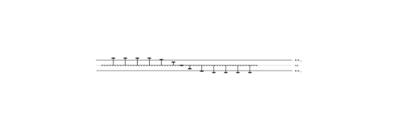
Figure 1: The system of pendulums: the view from above. The central dot represents a pendulum which is directed vertically upward. Lines $B_{1},\>B_{2}$ represent the two bounding rods, line $S$ represents the wire to which the pendulums are attached. The springs on the wire symbolize its torsional elasticity.

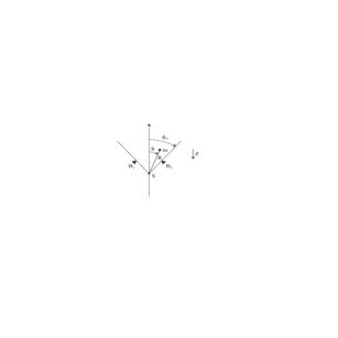
Figure 2: The perpendicular cross section of the system of pendulums. Only one pendulum is drawn. $B_{1},\>B_{2}$ and $S$ have the same meaning as in Fig.1.

The system described above reminds the one invented by A. C. Scott [4] in order to demonstrate sinus-Gordon solitons. Our system has very different properties due to the bounding rods.

When $\phi(x_{i},t)<\phi_{0}$ for all integer $i$ (notice the sharp inequality), equations of motion for the pendulums have the form

$$\ddot{\phi}(x_{i},t)=\frac{g}{R}\sin\phi(x_{i},t)+\kappa\frac{\phi(x_{i}-a,t)+\phi(x_{i}+a,t)-2\phi(x_{i},t)}{maR^{2}},$$ (1)

where the dots stand for derivatives with respect to the time $t$. The first term on the r.h.s. is due to the gravitational force acting on the mass $m$, and the second one represents the torque of the elastic forces exerted by the wire. The constant coefficient $\kappa$ characterizes the torsional elasticity of the wire.

Equation (1) is not valid when $\phi(x_{i},t)=\phi_{0}$ for certain pendulum because it does not include the instantaneous force acting on that pendulum from the bounding rod. The elastic bouncing condition has the form:

$$\dot{\phi}(x_{i},t)\rightarrow-\dot{\phi}(x_{i},t)$$

when $\phi(x_{i},t)=\pm\phi_{0}.$

We will consider Eq. (1) in the continuum limit. Standard steps, see, the first paper in [1], yield

$$\frac{\partial^{2}\phi(\xi,\tau)}{\partial\tau^{2}}-\frac{\partial^{2}\phi(\xi,\tau)}{\partial\xi^{2}}-\sin\phi(\xi,\tau)=0$$ (2)

when

$$|\phi(\xi,\tau)|<\phi_{0}.$$

Here we have introduced the dimensionless continuous variables:

$$\tau=\sqrt{\frac{g}{R}}\>t,\;\;\;\xi=\sqrt{\frac{mgR}{\kappa a}}\>x.$$

The elastic bouncing condition now takes the form

$$\frac{\partial\phi(\xi,\tau)}{\partial\tau}\rightarrow-\frac{\partial\phi(\xi,\tau)}{\partial\tau}\;\;\;\mbox{when}\;\;\;\phi(\xi,\tau)=\pm\phi_{0}.$$ (3)

Notice that Eq. (2) coincides with the well-known sinus-Gordon equation. In spite of that, it turns out that the condition (3) and the restriction

$$|\phi(\xi,\tau)|\leq\phi_{0}$$ (4)

change the dynamics dramatically.

Equation (2) and restriction (4) follow from the Lagrangian:

$$\;\;\;\;L=\frac{1}{2}(\partial_{\tau}\phi)^{2}-\frac{1}{2}(\partial_{\xi}\phi)^{2}-V(\phi),$$

where

$$V(\phi)=\left\{\begin{array}[]{lcl}\cos\phi-1&{\rm for}&|\phi|\leq\phi_{0},\\ \infty&{\rm for}&|\phi|>\phi_{0}.\end{array}\right.$$

This potential is shown in Fig. 3.

Figure 3: The field potential $V(\phi)$. The physical values of the field $\phi$ are restricted to the interval $[-\phi_{0},\phi_{0}].$

There are two degenerate ground states: $\;\phi=\pm\phi_{0}.$ The Lagrangian has the $Z_{2}$ symmetry $\phi\rightarrow-\phi$ which is spontaneously broken. Therefore we may expect that in this model there exists a topological defect represented by a static solution of field equation (2) interpolating between the two ground states. Indeed, such defect has been found, [1]. It is described in Section 3 below.

2.2 The folding transformation

The bouncing condition (3) implies that velocities of pendulums can be discontinuous functions of the time. One can get rid of this inconvenience by passing to an auxiliary model, which we shall call the ‘unfolded’ model. It is a new model with a field $\underline{\phi}(\xi,\tau)$ such that $\partial_{\tau}\underline{\phi}$ is continuous in $\tau$. As opposed to $\phi$, the new field $\underline{\phi}$ can take arbitrary real values. Solutions $\phi(\xi,\tau)$ of our original model are obtained from $\underline{\phi}(\xi,\tau)$ by formulas which correspond to multiple folding the $\underline{\phi}$ axis, see Fig. 4. Pertinent formulas can be found in paper [2].

Figure 4: The relation between $\phi$ and $\underline{\phi}.$

Figure 5: The field potential $\underline{V}(\underline{\phi})$ of the unfolded model. It is periodic function of $\underline{\phi}.$

It is clear from Fig. 4 that smooth motion along the $\underline{\phi}$ axis implies elastic reflection at $\pm\phi_{0}$ in the $\phi$ space. The field potential in the unfolded model is denoted by $\underline{V}(\underline{\phi})$. It has the form presented in Fig. 5.

The potential $\underline{V}(\underline{\phi})$ is symmetrically V-shaped at each minimum. The force $-d\underline{V}/d\underline{\phi}$ is always finite, hence the velocity $\dot{\underline{\phi}}$ does not have any discontinuities.

Because of its periodicity the potential $\underline{V}$ can be written in the form of Fourier series. Using such representation one can show that when $\phi_{0}\ll 1$ the unfolded model can be regarded as a nonanalytic perturbation of the sinus-Gordon model, [3].

The relation between the unfolded model and the original one reminds relation between a group and its universal covering.

2.3 The system of elastically coupled, vertically bouncing balls

Balls of mass $m$ can move along vertical poles which are fastened to a floor at the points $\xi_{i}=ai,\;i=0,\pm 1,\pm 2,\ldots,$ lying along a straight line. The balls bounce elastically from the floor, and each of them is connected with its nearest neighbors by elastic strings. The system has one degree of freedom per ball, represented by the elevation $\epsilon$ of the ball above the floor, see Fig. 6.

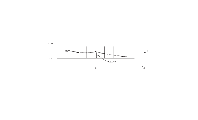
Figure 6: The system of balls connected by springs. The balls can move without friction along the vertical poles (the continuous vertical lines). They elastically bounce from the floor which is depicted as the continuous horizontal line.

Each ball is subject to the force of gravity and to the elastic forces from two strings. In a continuum limit equations of motion for this system can be written in the form

$$\frac{\partial^{2}\epsilon(\xi,\tau)}{\partial\tau^{2}}-\frac{\partial^{2}\epsilon(\xi,\tau)}{\partial\xi^{2}}=-1,$$ (5)

where $\epsilon(\xi,\tau)\geq 0.$

Here we use dimensionless variables $\tau,\xi$ and $\epsilon$. They differ from the dimensional ones by appropriate dimensional factors, [3].

The elastic bouncing condition has the from:

$$\frac{\partial\epsilon}{\partial\tau}(\xi,\tau)\rightarrow-\frac{\partial\epsilon}{\partial\tau}(\xi,\tau)\;\;\;\;\mbox{when}\;\;\;\;\epsilon(\xi,\tau)=0.$$

Similarly as in the case of pendulums, we can remove this cumbersome condition by unfolding the model. In the unfolded model, instead of the field $\epsilon(\xi,\tau)\geq 0$ we have a new field $\underline{\epsilon}(\xi,\tau)$ which can take arbitrary real values. The evolution equation for $\underline{\epsilon}$ has the form [3]

$$\frac{\partial^{2}\underline{\epsilon}(\xi,\tau)}{\partial\tau^{2}}-\frac{\partial^{2}\underline{\epsilon}(\xi,\tau)}{\partial\xi^{2}}=-\mbox{sign}(\underline{\epsilon}(\xi,\tau)),$$ (6)

where the sign function has the values $\pm 1$ when $\underline{\epsilon}\neq 0,$ and 0 if $\underline{\epsilon}=0.$ The corresponding field potential has the form

$$\underline{V}(\underline{\epsilon})=|\underline{\epsilon}|.$$ (7)

It has the regular symmetric V shape. The folding transformation has the form

$$\epsilon(\xi,\tau)=|\underline{\epsilon}(\xi,\tau)|.$$ (8)

3 The lack of exponential tails

Let us assume that the field equation has the following form

$$\frac{\partial^{2}\phi(\xi,\tau)}{\partial\tau^{2}}-\frac{\partial^{2}\phi(\xi,\tau)}{\partial\xi^{2}}+V^{\prime}(\phi)=0,$$ (9)

where the field potential $V(\phi)$ is V-shaped at the minimum located at $\phi=\phi_{0}.$ Hence, in the static case

$$\frac{\partial^{2}\phi(\xi)}{\partial\xi^{2}}-V^{\prime}(\phi)=0.$$ (10)

Suppose that $\phi$ approaches the constant ground state value $\phi_{0}$ from below ($\phi\rightarrow\phi_{0}-$). Then Eq. (10) is equivalent to the equation

$$\frac{\partial\phi(\xi)}{\partial\xi}=\sqrt{2\>(V(\phi)-V(\phi_{0}))}.$$

For $\phi$ close to $\phi_{0}$

$$\phi(\xi)=\phi_{0}-\delta\phi(\xi),$$

where $\delta\phi\geq 0,$ and

$$V(\phi)-V(\phi_{0})=-V^{\prime}(\phi_{0}-)\>\delta\phi+\frac{1}{2}V^{\prime\prime}(\phi_{0}-)\>(\delta\phi)^{2}+\ldots,$$

where $V^{\prime}(\phi_{0}-)$ denotes the limit of the first derivative from the side of $\phi<\phi_{0}$ (the left derivative of $V$ at $\phi_{0}$), $V^{\prime}(\phi_{0}-)<0.$ Hence, for $\delta\phi\cong 0$

$$\partial_{\xi}\delta\phi\cong-\sqrt{2|V^{\prime}(\phi_{0}-)|}\sqrt{\delta\phi}.$$

This equation has the general solution of the form

$$\delta\phi(\xi)\cong\frac{1}{2}|V^{\prime}(\phi_{0}-)|(\xi_{0}-\xi)^{2},$$ (11)

where $\xi_{0}$ is an arbitrary constant.

Thus, we have found a parabolic approach to the ground state value of the field $\phi$. This value is reached at $\xi=\xi_{0}$ exactly – there is no exponential tail. The parabolic approach is due to the fact that $V^{\prime}(\phi_{0}-)<0$. This means that the force pushing $\phi$ towards the ground state value does not vanish in the limit $\phi\rightarrow\phi_{0}-.$ In the two physical examples presented above this reflects the fact that there is a finite threshold for a force which could move the pendulums or the balls upward from the bounding line or the floor, respectively – the force has to be stronger than the gravity.

The well-known exponential tails are obtained when $V^{\prime}(\phi_{0})=0$ and $V^{\prime\prime}(\phi_{0})>0$. In that case

$$\delta\phi(\xi)\cong c_{0}\exp(-\sqrt{V^{\prime\prime}(\phi_{0})}\xi),$$

where $c_{0}$ is a constant.

Nice example of the parabolic approach to the ground state values of the fields is provivded by the topological defect found in the model with pendulums. Particularly simple is the case when the maximal allowed angle $\phi_{0}$ is small, $\phi_{0}\ll 1$. Then $\sin\phi\cong\phi,$ and Eq.(2) may be replaced by the linear one

$$\frac{\partial^{2}\phi(\xi,\tau)}{\partial\tau^{2}}-\frac{\partial^{2}\phi(\xi,\tau)}{\partial\xi^{2}}-\phi(\xi,\tau)=0.$$ (12)

However, one should keep in mind that this equation, as well as Eq.(2), is not physically relevant when $|\phi(\xi,\tau)|\geq\phi_{0}.$ The physically correct configuration is obtained by solving Eq.(12) when $|\phi|<\phi_{0}$ and matching this solution with the ground state fields $\pm\phi_{0}.$

Equation (12) has the static solution of the form $\phi_{0}\sin\xi$. Matching it with $\pm\phi_{0}$ yields the field $\phi_{c}(\xi)$ of the topological defect:

$$\phi_{c}(\xi)=\left\{\begin{array}[]{ccc}-\phi_{0}&\mbox{if}&\xi\leq-\pi/2\\ \phi_{0}\sin\xi&\mbox{if}&-\pi/2\leq\xi\leq\pi/2\\ +\phi_{0}&\mbox{if}&\xi\geq\pi/2.\end{array}\right.$$

In the case $\phi_{0}$ is not small $\sin\xi$ is replaced by an elliptic function. Then the matching with the ground states fields takes place at $\xi=\pm L/2$, where

$$L\cong\pi\left(1+\frac{\phi_{0}^{2}}{16}+\ldots\right)$$

when $\phi_{0}\ll 1,$ or

$$L\cong 2\ln\frac{4}{\pi-\phi_{0}}$$

when $\phi_{0}\rightarrow\pi-,$ see [1, 3].

Energy density for this topological defect reaches the exact vacuum value at $\xi=\pm L/2.$ For this reason we call the defect the ‘topological compacton’. In literature one can find other soliton or soliton-like solutions which have compact support, see, e.g., [5, 6, 7], but they are not related to topological sectors in field space. The name ‘compacton’ appears already in the paper [5].

Figure 7: The profile of the topological compacton when $\phi_{0}=1$. In this case $L/2\approx 1.67$.

Picture of the compacton in the system of pendulums is provided by Fig.1. There the compacton is seen from above. At the l.h.s. of the picture the pendulums just lie on the bounding rod $B_{1}$, more to the center they gradually rise above $B_{1}$, and at the r.h.s. of the picture they lie on the bounding rod $B_{2}$.

One consequence of the lack of exponential tails is that one can combine compactons and anti-compactons into a chain which is static, because these objects interact only when they touch each other. The anti-compacton is obtained by reversing the sign of the field $\phi_{c}$.

4 The asymptotic scale invariance

Let us consider small amplitude oscillations of the field $\phi$ around the V-shaped minimum of the field potential $V$ at $\phi=\phi_{0}:$

$$\phi(\xi,\tau)=\phi_{0}+\psi(\xi,\tau),$$

where $|\psi|\ll 1.$ For simplicity we put $\phi_{0}=0.$ Then Eq. (9) acquires the form

$$\frac{\partial^{2}\psi(\xi,\tau)}{\partial\tau^{2}}-\frac{\partial^{2}\psi(\xi,\tau)}{\partial\xi^{2}}+V^{\prime}(\psi)=0,$$ (13)

where the field potential $V(\psi)$ is V-shaped at the minimum located at $\psi=0,$ see Fig. 8.

Figure 8: Generic V-shaped potential and the piecewise linear approximation.

Because $\psi\approx 0,$ we may replace $V^{\prime}$ by its piecewise linear approximate form

$$V(\psi)\cong V^{\prime}(0+)\>\psi\>\Theta(\psi)-|V^{\prime}(0-)|\>\psi\>\Theta(-\psi),$$

where $\Theta$ denotes the step function. Then, Eq. (13) is replaced by

$$\frac{\partial^{2}\psi}{\partial\tau^{2}}-\frac{\partial^{2}\psi}{\partial\xi^{2}}=-V^{\prime}(0+)\>\Theta(\psi)+|V^{\prime}(0-)|\>\Theta(-\psi).$$ (14)

Notice that this equation remains nonlinear for arbitrarily small $\psi$ – there is no linear regime!

This equation has the scaling symmetry: if $\psi(\xi,\tau)$ is a solution of it, then

$$\psi_{\lambda}(\xi,\tau)\stackrel{{\scriptstyle df}}{{=}}\lambda^{2}\;\psi(\frac{\xi}{\lambda},\frac{\tau}{\lambda}),$$ (15)

where $\lambda>0$ is an arbitrary positive number, obeys Eq. (14) too. Because this symmetry appears in the approximate evolution equation (14) we call it the asymptotic scale invariance.

The energy

$$E[\psi]=\frac{1}{2}\int d\xi\>[(\partial_{\tau}\psi)^{2}+(\partial_{\xi}\psi)^{2}]+\int d\xi\>V(\psi)$$

scales as follows:

$$E[\psi_{\lambda}]=\lambda^{3}E[\psi].$$

In general, $\lambda$ should not be too large because if $\psi_{\lambda}$ has large amplitude then the piecewise linear approximation is not correct. This restriction does not apply to the unfolded mechanical model with bouncing balls because in that case the exact potential (7) is piecewise linear. When $\lambda\rightarrow 0+$ the solutions $\epsilon_{\lambda}(\xi,\tau)$ are in general characterized by high frequencies, short wave lengths and small energy. This reminds the phenomenon of turbulence, even more so when we recall that Navier-Stokes equations in the high Reynolds number regime have a scale invariance similar to the one described above.

Immediate consequence of the scale invariance is the lack of a characteristic frequency for small amplitude oscillations around the ground state. For example, one can find infinite periodic running wave solutions to Eq. (2) with the elastic bouncing condition (3) which have the dispersion relation of the form

$$\omega^{2}-k^{2}=\mu^{2},$$

where $\mu^{2}$ can take any value from the interval $(0,\infty),$ [1, 2].

Figure 9: The periodic running wave based on one bounding rod.

There are two kinds of such waves: with the pendulums bouncing periodically from one bounding rod, or swinging from one rod to the other one and back. In the former case the wave has the form presented in Fig. 9, where

$$\zeta=\frac{v\tau-\xi}{\sqrt{v^{2}-1}},$$

and $v>1$ is the phase velocity of the wave.

5 The self-similar solutions

We will discuss self-similar solutions of Eq. (14) in the particular case when $V^{\prime}(0+)=|V^{\prime}(0-)|.$ After rescaling $\xi$ and $\tau$ by $1/\sqrt{V^{\prime}(0+)}$ we obtain the following equation:

$$\frac{\partial^{2}\psi}{\partial\tau^{2}}-\frac{\partial^{2}\psi}{\partial\xi^{2}}=-\mbox{sign}(\psi).$$ (16)

It coincides with Eq.(6) of the unfolded model with the coupled balls. Direct physical meaning has $|\psi(\xi,\tau)|$ which is equal to the elevation above the floor of the ball at the point $\xi$ at the time $\tau$.

We follow the standard procedure for finding the self-similar solutions, see, e.g., [8]. In our case the appropriate Ansatz for the solution has the form

$$\psi(\xi,\tau)=\xi^{2}S(y),\;\;\;y=\frac{\tau}{\xi}.$$

Then Eq.(16) is reduced to the ordinary differential equation for the function $S(y)$

$$(1-y^{2})\>S^{\prime\prime}+2y\>S^{\prime}-2\>S=-\mbox{sign}(S).$$

This equation has the following partial solutions:

$$\mbox{when}\;\;\;S>0:\;\;\;\;\;\;S(y)=-\frac{1}{2}\beta(y^{2}+1)+\frac{\alpha}{2}y+\frac{1}{2},$$

$$\mbox{when}\>\;\;S<0:\;\;\;\;\;\;S(y)=\frac{1}{2}\beta(y^{2}+1)-\frac{\alpha}{2}y-\frac{1}{2},$$

$$S(y)=0,$$

where $\alpha,\beta$ are constants. These partial solutions are valid on appropriate finite intervals of the $y$-axis. They are put together to form the complete solution, [3]. To this end one has to solve recurrence relations obtained from infinite number of matching conditions. One parameter remains free, so we actually obtain a family of self-similar solutions. Example of the solution is depicted in Fig. 10.

Figure 10: The self-similar solution. The two arrows indicate that the waves emanate from the points which move along the $\xi$-axis: $\xi=\pm\tau$.

The solution is composed of infinitely many quadratic polynomials in $\xi$ taken on domains which become smaller and smaller when $\xi\rightarrow\tau+$ or $\xi\rightarrow-\tau-$. For $\xi\rightarrow\pm\infty$ and fixed $\tau>0$ the solution approaches the linear functions $\pm\tau\xi/2.$ The zeros of $\psi$ move with ‘super luminal’ velocities, that is with velocities greater than 1.

The solution presented in Fig. 10 is symmetric with respect to $\xi\rightarrow-\xi.$ It turns out that the left- and right-hand halves of this solution taken separately are solutions too.

The solution described above cannot be physically realized in the system of coupled balls because it has infinite energy – this is a general feature of self-similar solutions. Nevertheless, finite pieces of it can be observed. The point is that the dynamics of the model is local. Therefore, if a physical, finite energy initial configuration differs from our solution only at very large values of $|\xi|$, this difference will be seen in the region of finite $|\xi|$ only after certain finite time interval. During that time interval the self-similar solution describes the evolution of the part of the system very well.

6 The symmetric shock waves

These solutions are not of the self-similar type. The Ansatz

$$\psi(\xi,\tau)=\Theta(-z)W(z),\;\;\;\;\mbox{where}\;\;\;\;z=\frac{1}{4}(\xi^{2}-\tau^{2})$$

reduces Eq. (16) to the following ordinary differential equation

$$z\>W^{\prime\prime}+W^{\prime}=\mbox{sign}(W),$$

which has the following partial solutions:

$$\mbox{when}\;\;\;W>0:\;\;\;\;W(z)=z+z_{1}+z_{1}\>\ln|\frac{z}{z_{1}}|+d_{1},$$

$$\mbox{when}\;\;\;W<0:\;\;\;\;W(z)=-z-z_{0}-z_{0}\>\ln|\frac{z}{z_{0}}|-d_{0},$$

where $d_{0},d_{1},z_{0},z_{1}$ are constants. These solutions are defined on finite intervals of the $z$-axis. Putting them together we obtain a one parameter family of solutions which are defined for all $z\leq 0$, [3]. Because of the step function in the Ansatz we do not need to know $W(z)$ for $z>0.$

$\Theta(-z)W(z)$ describes a shock wave, symmetric with respect to $\xi\rightarrow-\xi$ and restricted to the light-cone $\xi^{2}\leq\tau^{2}.$ The snapshots of the wave at three times are shown in Figs. 11, 12, 13.

Figure 11: The symmetric shock wave at an initial time $\tau_{0}>0$. The arrows indicate that the wave fronts move. $\psi(\xi,\tau_{0})=0$ for $|\xi|>\tau_{0}.$

Figure 12: The symmetric shock wave at a time $\tau_{1}>\tau_{0}.$ Now $\psi(\xi,\tau_{1})=0$ for $|\xi|>\tau_{1}.$

Figure 13: The symmetric shock wave at a time $\tau_{2}>\tau_{1}.$ At later times more zeros of $\psi$ appear.

The height of the step, equal to $W(0)$, is the free parameter. The velocities of the steps (shock fronts) are equal to $\pm 1$. The number of zeros of the function $\psi$ grows indefinitely with the time $\tau.$ These zeros move along the $\xi$-axis with velocities larger that 1, but they never catch up with the front.

The shock wave described above has infinite energy because the gradient energy density at the shock fronts is infinite. In a real physical system like the system of coupled balls this energy will be finite, but then our solution is only an approximation to the real dynamics. Certainly it can be helpful, but it should be used with care.

7 Summary

Let us list the main features of classical field-theoretic models with the V-shaped potentials that we have found:

• the parabolic approach to the ground state value of the field,

• the absence of linear regime for oscillations around the ground state,

• the (approximate) scale invariance and the existence of self-similar solutions,

• the existence of shock waves.

These ‘signatures’ may help to find physical realizations of such models other than the classical mechanical systems of the type presented in Section 2.

There are several interesting questions which in our opinion deserve attention.
1. How does the presence of the threshold force, which is the reason for the lack of exponential tails, influence the evolution of finite energy perturbations of the ground state?
2. The continuum limit yields models which in general are much simpler than the discrete ones, see, e.g., remarks in [9]. What are the physical properties of discrete systems with V-shaped potentials? In particular, is there a discrete version of the shock wave in the system of coupled balls?
3. What are the properties of the corresponding quantum models ? In particular, one may expect that the scale invariance will be broken in the quantum model. What is the resulting mass scale?

We hope to provide some partial answers soon.

8 Acknowledgements

H. Arodź and P. Klimas thank the Organizers of the School for their very kind hospitality, and for the possibility to present this lecture (H. A.).

This work is supported in part by the COSLAB Programme of the European Science Foundation.

References

- [1] H. Arodź, Acta Phys. Pol. B33 (2002) 1241 (nlin.ps/0201001); B35 (2004) 625 (hep-th/0312036)
- [2] H. Arodź and P. Klimas, Acta Phys. Pol. B36 (2005) 787 (cond-mat/0501112)
- [3] H. Arodź, P. Klimas and T. Tyranowski, in preparation.
- [4] A. C. Scott, Amer. J. Phys. 37 (1969) 52.
- [5] P. Rosenau, J. M. Hyman, Phys. Rev. Lett. 70 (1993) 564.
- [6] F. Cooper, H. Shepard and P. Sodano, Phys. Rev. E48 (1993) 4027.
- [7] S. Dusuel, P. Michaux and M. Remoissenet, Phys. Rev. E57 (1998) 2320.
- [8] L. Debnath, Nonlinear Partial Differential Equations for Scientists and Engineers. Birkhäuser, Boston-Basel-Berlin, 2005. Chapter 8.
- [9] M. Remoissenet, Waves Called Solitons. Concepts and Experiments. Springer-Verlag, Berlin-Heidelberg-New York, 1996. Chapter 6.