SU-ITP-05/30 IPM/P-2005/037 hep-th/0510189

Integrable Spin Chains on the Conformal Moose

$\mathcal{N}=1$ Superconformal Gauge Theories as
Six-Dimensional String Theories

Darius Sadri¹, M. M. Sheikh-Jabbari²

¹Department of Physics, Stanford University
382 via Pueblo Mall, Stanford CA 94305-4060, USA

²Institute for Studies in Theoretical Physics and Mathematics (IPM)
P.O.Box 19395-5531, Tehran, Iran

darius@itp.stanford.edu, jabbari@theory.ipm.ac.ir

Abstract

We consider ${\cal N}=1,\ D=4$ superconformal $U(N)^{p\times q}$ Yang-Mills theories dual to $AdS_{5}\times S^{5}/Z_{p}\times Z_{q}$ orbifolds. We construct the dilatation operator of this superconformal gauge theory at one-loop planar level. We demonstrate that a specific sector of this dilatation operator can be thought of as the transfer matrix for a two-dimensional statistical mechanical system, related to an integrable $SU(3)$ anti-ferromagnetic spin chain system, which in turn is equivalent to a $2+1$-dimensional string theory where the spatial slices are discretized on a triangular lattice. This is an extension of the $SO(6)$ spin chain picture of ${\cal N}=4$ super Yang-Mills theory. We comment on the integrability of this ${\cal N}=1$ gauge theory and hence the corresponding three-dimensional statistical mechanical system, its connection to three-dimensional lattice gauge theories, extensions to six-dimensional string theories, AdS/CFT type dualities and finally their construction via orbifolds and brane-box models. In the process we discover a new class of almost-BPS BMN type operators with large engineering dimensions but controllably small anomalous corrections.

1 Introduction

According to AdS/CFT [1, 2] string theory on a given background (which is a gravitating theory) is dual to a (usually non-gravitational) gauge theory. The best known example of this duality is between type IIB strings on $AdS_{5}\times S^{5}$ with $N$ units of the fiveform flux on $S^{5}$ and the four dimensional $\mathcal{N}=4$ $U(N)$ supersymmetric Yang-Mills (SYM) theory. The latter has a vanishing $\beta$-function and is a conformally invariant field theory. As a superconformal field theory the perturbative quantum corrections appear only through the anomalous dimensions of operators. Hence solving the field theory amounts to specifying the scaling dimensions of the operators (up to some conformal ratios). The scaling dimension $\Delta$ of a given operator ${\cal O}_{\Delta}$ is the eigenvalue of the dilatation operator ${\mathfrak{D}}$, i.e.

$$[{\mathfrak{D}},{\cal O}_{\Delta}]=\Delta{\cal O}_{\Delta}\ .$$ (1.1)

The dilatation operator ${\mathfrak{D}}$ is the Hamiltonian of the ${\cal N}=4$ gauge theory on $\mathbb{R}\times S^{3}$ or equivalently the Hamiltonian of the gauge theory on $\mathbb{R}^{4}$ in radial quantization [2]. Therefore, giving a representation of ${\mathfrak{D}}$ on the space of fields of the ${\cal N}=4$ gauge theory (the constituents of ${\cal O}_{\Delta}$) amounts to solving the theory.

In the last two years, motivated by the results and insights obtained from the BMN [3] double scaling limit (for reviews see [4, 5]) some very important steps towards determining the dilatation operator ${\mathfrak{D}}$ were taken [6, 7]. The original observation was made realizing a close connection between the dilatation operator ${\mathfrak{D}}$ in some specific subsector of the operators of the gauge theory and the Hamiltonian of an integrable system, namely the $SO(6)$ spin chain system [8]. Based on this observation it was proposed that the ${\cal N}=4$ gauge theory is also integrable (in a certain limit). This proposal is based on two facts:
    (i) There is a one-to-one correspondence between the gauge invariant operators of the ${\cal N}=4$ gauge theory which are built strictly from $\Delta_{0}$ number of (six real) scalars of the ${\cal N}=4$ gauge multiplet and the allowed configurations of an $SO(6)$ spin chain system with $\Delta_{0}$ number of sites. Verification of this observation is almost immediate.
    (ii) At planar, one-loop level, i.e.​ strict ’t Hooft large $N$ limit and at first order in the ’t Hooft coupling $g_{YM}^{2}N$, the one-loop anomalous correction to the dilatation operator obtained via explicit computations of two-point functions matches exactly the Hamiltonian of an $SO(6)$ spin chain system with nearest neighbor interactions; for a nice review on this subject see [9].

The above observations were extended beyond the $SO(6)$ sector to the one-loop planar dilatation operator of the full theory [6], which matches the Hamiltonian of a “super spin chain” system [10]. The above has been checked by explicit computations of two-point functions. In fact it has been shown that the four-dimensional superconformal invariance under $psu(2,2|4)$ is strong enough to completely fix the form of the dilatation operator at one-loop planar level [9].

To argue for the integrability of the ${\cal N}=4$ SYM, even in the strict ’t Hooft planar limit, one needs to know all loop results. In this direction the higher loop planar dilatation operator has been worked out in [14, 15], where it was argued that the integrability structure survives. As a result of technical difficulties, these computations have been mainly limited to some subsectors of the $SO(6)$ sector. At higher-loop level, although still very restrictive, the superconformal symmetry is not enough to completely fix the form of the dilatation operator [9] and some explicit computation is necessary. These computations, on the gauge theory side, have been performed mainly in the BMN or near BMN limit [14, 15] corresponding to the thermodynamic limit of the spin chain system where the Bethe ansatz [16] is applicable [9]. At higher-loop level the corresponding spin chain system is not of the form of nearest neighbor interactions. So far the dilatation operator has been worked out up to four-loop planar level; at three-loop level some discrepancies with the results of the string theory side have been observed [9, 17] and more recently it has been argued that these discrepancies can be resolved using the “quantum string Bethe ansatz” [18].

In this work we consider the less supersymmetric cases of ${\cal N}=1$ superconformal gauge theories and extend the results of the spin chain/gauge theory correspondence to these cases. The example of interest here is the ${\cal N}=1,\ D=4$ $U(N)^{p\times q}$ SYM with $3\,p\,q$ chiral matter fields in the bi-fundamental representations $(N_{ij},\bar{N}_{i+1,j})$, $(N_{ij},\bar{N}_{i,j+1})$ and $(N_{i+1,j},\bar{N}_{i,j+1})$, with $i=1,2,\cdots,p$, $j=1,2,\cdots,q$. This gauge theory is dual to type IIB strings on the $1/8$ BPS orbifold of $AdS_{5}\times S^{5}$ [23, 24, 25]. We find the dilatation operator of this SCFT and argue for the integrability of the ${\cal N}=1$ theory in the appropriate limit [27, 28], which we find to extend beyond the untwisted states that result from large $N$ orbifold inheritance [24, 25]. A similar analysis for ${\cal N}=2$ superconformal gauge theories has been carried out in [29]. (Penrose limits of such orbifolds have been studied in [30].)

One of our remarkable results is that we find a three-dimensional classical statistical mechanical system whose Euclidean spatial slices form the quiver (moose) diagram [23] describing the orbifold gauge theory, which for the case of interest is a two-dimensional triangular lattice. We will argue that our system is equivalent to a $2+1$ dimensional $U(N)$ lattice gauge theory. This in turn is equivalent to a $2+1$ dimensional string theory with discretized worldsheet and target space. The thermodynamic limit then corresponds to taking $N$ large. The latter brings a new insight into the spin chains related to the ${\cal N}=4$ gauge theory.

In section 2, we outline the structure of the lattice, the transformation properties of the bi-fundamental fields, enumerate the gauge invariant operators and describe their structure on the lattice. In section 3, we work out the dilatation operator of the $\mathcal{N}=1$ orbifold theory. We demonstrate that the dilatation operator can be thought of as the transfer matrix for a theory on the corresponding $2d$ lattice. In section 4, we discuss two different views of the structure we uncover: a description in terms of a lattice Laplacian which makes manifest the string dynamics and a description in terms of an integrable spin chain. We also make some comments on the BMN limit of the ${\cal N}=1$ superconformal theory. In section 5, we discuss how the $2+1$-dimensional lattice picture is extended to a $3+2+1$ dimensional string theory, once the gauge fields of the ${\cal N}=1$ theory are also included. For this purpose we use a relation between AdS/CFT and brane box models [31]. In section 6, we discuss the Higgsed phase of the ${\cal N}=1$ theory, where the conformal symmetry is lost. In this section we discuss the relation to $2+1$ dimensional lattice gauge theories as well as the deconstruction and six-dimensional picture. Finally in section 7 we give a summary and outlook. In two appendices we introduce and fix our conventions, and give some examples to clarify the discussion in the main body of the work.

2 ${\cal N}=1$ Gauge Theory and the Lattice

In this section we introduce and elaborate on a pictorial way of presenting the ${\cal N}=1$ SYM theory, an interesting subset of its operators and the dilatation operator, using the corresponding quiver diagram, which in our case is a two dimensional triangular lattice. This two dimensional lattice plays a central part in our construction, and its role as a target space for string dynamics will become apparent as we proceed.

2.1 The Lattice

The field content of the $\mathcal{N}=1$ supersymmetric gauge theory is given by a triplet of chiral supermultiplets, which we label as $A,B,C$. These arise as orbifold projections of the three chiral multiplets of $\mathcal{N}=4$ theory when written in $\mathcal{N}=1$ language. In addition, we have a single vector supermultiplet, again projected from the vector multiplet of the parent $\mathcal{N}=4$ theory.

The projected fields transform non-trivially under the $U(N)^{p\times q}$ subgroup of the original $U(Npq)$ gauge symmetry of the ${\cal N}=4$ theory which survives the orbifolding. This subgroup consists of the degrees of freedom left invariant by the orbifold action. To construct the $\mathbb{Z}_{p}\times\mathbb{Z}_{q}$ orbifold theory we start with an ${\cal N}=4$ $U(Npq)$ theory and then find an $Npq\times Npq$ representation of $\mathbb{Z}_{p}\times\mathbb{Z}_{q}$ under which the chiral multiplets are projected to $3pq$ $N\times N$ matrices, in bi-fundamental representations of the $U(N)^{p\times q}$ [24, 25].

The three complex scalars are bi-fundamentals under this gauge symmetry, and are to be associated with directed links on the lattice, the indices $i,j$ denoting the particular gauge group associated with a lattice site.

The transformation properties are as follows:

$$A_{i,j} \>\>\>\>\>\>\>\>\sim\>\>\>\>\>\>\>\left(N_{i,j}\ ,\ \>\bar{N}_{i,j+1}\right)\>\>,$$ (2.1a)

$$B_{i,j} \>\>\>\>\>\>\>\>\sim\>\>\>\>\>\>\>\left(N_{i,j}\ ,\ \>\bar{N}_{i-1,j-1}\right)\>\>,$$ (2.1b)

$$C_{i,j} \>\>\>\>\>\>\>\>\sim\>\>\>\>\>\>\>\>\left(N_{i,j}\ ,\ \bar{N}_{i+1,j}\right)\>\>.$$ (2.1c)

The first entry gives the starting point of the directed link and the second entry the endpoint. Conjugation of a field corresponds to flipping the direction of the arrow on a link, yielding the transformation properties for the conjugate fields:

$$\bar{A}_{i,j} \>\>\>\>\>\>\>\>\sim\>\>\>\>\>\>\>\left(N_{i,j+1}\ ,\ \ \ \>\bar{N}_{i,j}\right)\>\>,$$ (2.2a)

$$\bar{B}_{i,j} \>\>\>\>\>\>\>\>\sim\>\>\>\>\>\>\>\left(N_{i-1,j-1}\ ,\ \bar{N}_{i,j}\right)\>\>,$$ (2.2b)

$$\bar{C}_{i,j} \>\>\>\>\>\>\>\>\sim\>\>\>\>\>\>\>\left(N_{i+1,j}\ ,\ \ \ \>\bar{N}_{i,j}\right)\>\>.$$ (2.2c)

On the lattice, the fields in the vector multiplet $V$ of the ${\mathcal{N}=1}$ theory are associated with lattice sites, as they are adjoints whose transformation property is:

$$V_{i,j}\>\>\>\>\>\>\>\>\sim\>\>\>\>\>\>\>\left(N_{i,j}\ ,\ \bar{N}_{i,j}\right)\>\>.$$ (2.3)

The gauge structure of the theory after orbifolding is captured succinctly by a moose (or quiver) diagram [23], whose structure gives a visualization of the transformation properties of the fields which survive the orbifold, as given above. For the orbifold under consideration the relevant moose is a two-dimensional triangular lattice, with $p\times q$ sites. The coordinates on the lattice as well as the basis vectors are depicted in Figures 1 and 2.

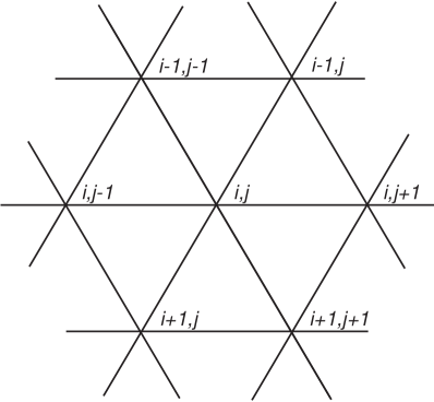
Figure 1: The lattice coordinates.

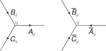
Figure 2: The direction vectors designating the three chiral multiplets on the lattice, relative to the site $i,j$.

In other words, our two dimensional lattice is on a torus and the volume of the torus is proportional to $pq$; that is a fuzzy two torus with the fuzziness parameter $\Theta=\frac{r}{pq}$, where $r={\rm gcd}(p,q)$ is the greatest common divisor of $p$ and $q$; for $p=q$, $\Theta=1/p$. One should, however, note that the lattice spacing and the size of the links is an arbitrary scale in the conformal field theory. For this reason we have called this lattice a “conformal moose” (recall the expression in the title). This means that for the fuzzy torus we are considering the complex structure is fixed and the ratio of the real and imaginary parts of the Kahler form, $\Theta$, is also fixed. In section 6 we consider a case where the size of the lattice spacing is fixed, by giving VEV’s to the bi-fundamental scalars.

The ratio of the coupling of the orbifolded gauge theory to the parent theory depends on the order of the finite group generating the orbifold, in our case $\mathbb{Z}_{p}\times\mathbb{Z}_{q}$. After orbifolding, the coupling of the $\mathcal{N}=1$ theory is related to the parent theory’s coupling by

$$g_{YM}^{2}=(g_{YM}^{parent})^{2}\times p\times q$$ (2.4)

where the order of the orbifold group appears on the right hand side.

The superpotential of the theory can also be calculated using e.g. the techniques of [31]:

$$W=\sum_{i=1}^{p}\sum_{j=1}^{q}\ tr\left(A_{ij}B_{i,j+1}C_{i-1,j}-A_{ij}C_{i,j+1}B_{i+1,j+1}\right),$$ (2.5)

where the $tr$ is over the $N\times N$ matrices and $A,B$ and $C$’s now represent the three bi-fundamental chiral superfields. This superpotential has a simple representation on the $2d$ oriented triangle lattice: sum over all the basic cells on the lattice (triangles), with a charge assignment, positive sign to counter-clockwise loops and negative sign to clockwise ones.

2.2 Gauge Invariant Operators

The observables of the ${\mathcal{N}=1}$ theory we focus on are constructed as gauge invariant combinations of the degrees of freedom. We shall be primarily interested in those operators built from the three complex scalar fields which in ${\mathcal{N}=1}$ language correspond to the scalar components of the three chiral superfields. The group structure of the fields will be responsible for much of the interesting physics we discuss, and so apply with little change to the fermions in the chiral multiplets. We also briefly mention how the vector multiplet enters the picture.

Given the transformation properties of the fields, we are not free to multiply them arbitrarily. Any gauge invariant operator is the trace of an appropriate combination of fields, or the product of several such traces. As is evident, any gauge invariant operator is mapped onto a certain closed loop on the lattice, one loop being associated to each trace. Among the closed loop operators there exist distinguished classes, for example those which are BPS, or those constructed only from chiral fields $A,B,C$, and not their conjugates. We shall refer to the latter as “holomorphic” operators, which include as a subclass the BPS operators. We caution the reader that not all “holomorphic” operators as defined are protected, and to avoid confusion, we shall take care to distinguish between “BPS” and “holomorphic”. We will show in the next section that the BPS protected operators are those built only from a single chiral or anti-chiral multiplet, for example a string of $A$’s, and by virtue of gauge invariance must completely wrap the lattice in one direction. They can of course wrap multiple times; the important point is that they begin and end at the same site.

The most general operator consisting only of scalar fields contains both chiral and anti-chiral fields. The chiral fields are assigned with positive $R$-charge, whereas the anti-chiral ones carry opposite or negative $R$-charge, as per usual in $\mathcal{N}=1$ supersymmetry. We use the convention that the $R$-charge of a fundamental chiral field is one. The $U(1)$ R-symmetry of the orbifold theory is a subgroup of the $SO(6)_{R}\simeq SU(4)_{R}$ of the parent theory. In fact the subgroup surviving the orbifolding is larger, i.e. $U(1)\times\mathbb{Z}_{p}\times\mathbb{Z}_{q}$, where is $\mathbb{Z}_{p}\times\mathbb{Z}_{q}$ is known as “quantum symmetry” [25] and on the lattice is nothing but the translations on the (fuzzy) two torus. As we will see later, when we reinterpret the dilatation operator as a Hamiltonian, the $R$-charge is a conserved quantity.

There is a straightforward way to understand which operators survive the orbifolding. The operators we have described fall into two classes, depending on whether they are inherited from the parent $\mathcal{N}=4$ theory or not, i.e.​​ untwisted or twisted respectively. Given an operator in the daughter theory, the question of whether the operator is inherited can be recast in terms of its charge under the quantum symmetry. The generators of the $\mathbb{Z}_{p}\times\mathbb{Z}_{q}$ quantum symmetry generate translations along the two dimensional lattice. On the covering space the generators of $U(N)$ are tensored with the generators of $\mathbb{Z}_{p}\times\mathbb{Z}_{p}$ (taking $q=p$) and the gauge-invariant operators are traces of products of fields sitting in the product representation $U(N)\otimes\Gamma_{i}\otimes\tilde{\Gamma}_{j}$ with $\Gamma_{i}$ and $\tilde{\Gamma}_{j}$ the generators of the first and second $\mathbb{Z}_{p}$ factor respectively, and $i,j=1,2,\cdots,p$. The traces from which gauge-invariant operators are built are understood as acting on these tensor products. Not all such products have non-vanishing trace, and there are many gauge-invariant operators in the parent theory which are projected out by the orbifold action. Those which are traceless are precisely the operators which do not survive the orbifolding. Examples of such operators (for the case of a $\mathbb{Z}_{3}\times\mathbb{Z}_{3}$ orbifold) are $Tr(A^{2})$, $Tr(AB)$, and $Tr(ABA)$, with $A,B,C,\bar{A},\bar{B},\bar{C},$ the fields of $\mathcal{N}=4$ $U(Npq)$ supersymmetric theory written as three complex fields (as we do when writing the action for this theory in $\mathcal{N}=1$ language). Some examples of operators which survive the projection are $Tr(A^{3})$, $Tr(A^{6})$, $Tr(ABC)$, and $Tr(ABABAB)$. Take for example $Tr(ABC)$. Carrying out the projection, this gives rise to

$$\sum_{i,j}\ tr\left(A_{i,j}B_{i,j+1}C_{i-1,j}\right)$$

where $tr$ is now the trace over $U(N)$ valued fields. The sum in this expression places one such operator starting at each lattice site, and hence this operator covers the entire lattice in a symmetric manner. It is invariant under shifts along any lattice direction (the quantum symmetry) and the operators which are invariant under this symmetry are precisely the inherited untwisted operators. The Hamiltonian of the $\mathcal{N}=1$ superconformal Yang-Mills theory, its superpotential (2.5), as well as the dilatation operator are in this sector of the theory. Likewise there are operators which appear in the $\mathcal{N}=1$ projected theory which are not inherited from the parent. This second class constitutes the operators forming the twisted sector of the theory. The twisted operators are those which are not invariant under the quantum symmetry (lattice translations), so for example $tr\left(A_{i,j}B_{i,j+1}C_{i-1,j}\right)$ without a sum on $i,j$, sits in the twisted sector. It is also evident that not all BPS operators in the daughter theory are descendants of chiral primary operators in the parent $\mathcal{N}=4$ theory. An operator of the form $tr(A_{i,j}A_{i,j+1}\ldots A_{i,j+p})$ which wraps the lattice once along a single horizontal line is not inherited, but if we replicate it along all horizontal lines, $\sum_{i}tr(A_{i,j}A_{i,j+1}\ldots A_{i,j+p})$, then it can be related to an $\mathcal{N}=4$ chiral primary.

There is another classification of the operators on the lattice which comes from the fact that the lattice is on a torus. As we argued above the gauge invariant operators are orientable close loops on the lattice, they can then be shrinkable or non-shrinkable cycles of the (fuzzy) two torus. For example, the operator $tr\left(A_{i,j}B_{i,j+1}C_{i-1,j}\right)$ is shrinkable whereas $tr(A_{i,j}A_{i,j+1}\ldots A_{i,j+p})$ is a non-shrinkable one. One can associate a “winding” number to non-shrinkable operators. We will comment more on this point in section 4.

We would like to also point out that, in the 2+1-dimensional picture given here, one may introduce Wilson lines to generate gauge invariant operators that cover all six dimensions, by extending our loops to also include loops that extend into the 3+1-dimensional space-time. The idea is to take a composite operator, sitting at $x$, and explode it into pieces sitting at different space-time points, with Wilson lines running from space-time point to space-time point between the sub-operators at the different points to make the whole operator gauge invariant. Then we have a loop that lies in 3+1+2 dimensions. The dilatation/Hamiltonian operator is then a direct sum of the 3+1-dimensional one and the one on the lattice (to be discussed in the next section).

3 Gauge Theory Dynamics on the Lattice

So far we have built a one-to-one relation between the gauge invariant operators of a $U(N)^{p\times q}$ ${\cal N}=1$ superconformal gauge theory which are made out of $3pq$ bi-fundamental scalars and the oriented closed loops on the $2d$ triangle lattice, which wraps a fuzzy two torus. Here we extend the lattice description of the ${\cal N}=1$ SCFT to beyond the level of operators and Hilbert spaces, to a dynamical level and in section 3.2 present a simple lattice description of the terms in the one loop planar dilatation operator.

3.1 Dilatation operator of the ${\cal N}=1$ gauge theory

In this section we work out the dilatation operator of the $\mathcal{N}=1$ superconformal gauge theory, in the subsector of operators built purely from the three complex scalars. We present a derivation via an orbifolding of the $\mathcal{N}=4$ dilatation operator, but also outline a more direct derivation starting from the $\mathcal{N}=1$ action.

The $\mathcal{N}=4$ dilatation operator up to two-loop order and at planar-level for operators built strictly from scalars (and no covariant derivatives) has been worked out in [6]. We quote the one-loop result here, which we take as a starting point for the derivation of the dilatation operator in the $\mathcal{N}=1$ theory. This theory contains six real scalars transforming in the adjoint representation of the $U(Npq)$ gauge group and the fundamental of the $SO(6)$ R-symmetry of the $\mathcal{N}=4$ theory, which we collect into three complex scalars making manifest an $SU(3)$ subgroup of $SO(6)$.

The dilatation operator $\mathfrak{D}$ has a perturbative expansion in powers of the Yang-Mills coupling constant $g_{YM}$, taking the form

$$\mathfrak{D}=\sum_{n=0}^{\infty}\left(\frac{g_{YM}}{4\pi}\right)^{2n}\mathfrak{D}_{n}\>\>.$$ (3.1)

Here $\mathfrak{D}_{n}$ is the $n$-loop contribution. The eigenvectors of $\mathfrak{D}$ are the operators with well defined scaling dimensions, given by their respective eigenvalues. In general at higher-loops $\mathfrak{D}$ is not diagonal due to operator mixing, and finding a suitable basis of scaling operators requires diagonalizing $\mathfrak{D}$ at the appropriate loop order. The tree level (classical) scaling dimension is $\mathfrak{D}_{0}$, which is given by

$$\mathfrak{D}_{0}=\sum_{m=1}^{6}Tr:\phi_{m}\ \delta_{m}:\>\>,$$ (3.2)

where $:\ :$ denotes normal ordering, taken here to mean that all the variations with respect to the fields are understood not to act on other fields within the same $:\ :$ block.

The one-loop correction to the scaling is given by (after extracting the coupling dependent prefactor)

$$\mathfrak{D}_{1}\>=\>-\sum_{m=1}^{6}\sum_{n=1}^{6}Tr:\left([\phi_{m},\phi_{n}][\delta_{m},\delta_{n}]+\frac{1}{2}[\phi_{m},\delta_{n}][\phi_{m},\delta_{n}]\right):\>\>.$$ (3.3)

The ordering of the fields is important because of their matrix structure. As explained in Appendix A, the derivatives which appear above are a short-hand way of capturing the action of Wick contractions, leading to propagators.

The one-loop dilatation operator, when expressed in terms of the complex scalars, can be split into three parts,

$$\mathfrak{D}_{1}\>=\>\mathfrak{D}_{1}^{h}\>+\>\mathfrak{D}_{1}^{\bar{h}}\>+\>\mathfrak{D}_{1}^{h\bar{h}}\>\>,$$ (3.4)

with

$$\begin{split}\mathfrak{D}_{1}^{h}=&-\sum_{i=1}^{3}\sum_{j=1}^{3}Tr\Big{(}[\Phi_{i},\Phi_{j}][\Delta_{i},\Delta_{j}]\Big{)}\>\>,\\ \mathfrak{D}_{1}^{\bar{h}}=&-\sum_{i=1}^{3}\sum_{j=1}^{3}Tr\Big{(}[\bar{\Phi}_{i},\bar{\Phi}_{j}][\bar{\Delta}_{i},\bar{\Delta}_{j}]\Big{)}\>\>,\\ \mathfrak{D}_{1}^{h\bar{h}}=&-\sum_{i=1}^{3}\sum_{j=1}^{3}Tr\Big{(}2[\Phi_{i},\bar{\Phi}_{j}][\Delta_{i},\bar{\Delta}_{j}]+[\Phi_{i},\Delta_{j}][\bar{\Phi}_{i},\bar{\Delta}_{j}]+[\Phi_{i},\bar{\Delta}_{j}][\bar{\Phi}_{i},\Delta_{j}]\Big{)}\>\>.\end{split}$$ (3.5)

The significance of explicitly splitting the dilatation operator in this way will become clear momentarily. Here $\mathfrak{D}_{1}^{h}$ denotes the parts of the dilatation operator constructed only from holomorphic fields and derivatives, and likewise $\mathfrak{D}_{1}^{\bar{h}}$ with holomorphic fields and derivatives replaced by anti-holomorphic ones. Finally, $\mathfrak{D}_{1}^{h\bar{h}}$ contains mixed holomorphic and anti-holomorphic terms. Certain subsectors of operators are not mixed under renormalization; the example of our interest is the sector of holomorphic operators which is closed. This is due to the fact that $\mathfrak{D}_{1}^{\bar{h}}$ and $\mathfrak{D}_{1}^{h\bar{h}}$ vanishes on the holomorphic operators and the action of the dilatation operator on holomorphic operators receives contributions only from $\mathfrak{D}_{1}^{h}$.

To obtain the dilatation operator of the ${\cal N}=1$ theory we perform the orbifolding on (3.5). The justification why this procedure should work comes from the fact that the dilatation operator of the ${\cal N}=1$ theory is in the untwisted sector and hence is directly inherited from the parent theory [25]. To perform the orbifolding, we expand the fields and the variations in equation (3.5) in a basis of the orbifolded generators $\Phi_{I}=\Phi_{I}^{a}T^{a},\Delta_{I}=\Delta_{I}^{a}\bar{T}^{a}$ (as explained in Appendix B; see also Appendix A for why $\Delta_{I}$ is taken to transform as the conjugate of $\Phi_{I}$), then collect terms after evaluating the trace. Here $a$ enumerates the hermitian generators of $U(Npq)$.

Carrying out the projection for a general $\mathbb{Z}_{p}\times\mathbb{Z}_{p}$ orbifold (i.e.​ taking $q=p$), we arrive at a sum of terms, whose structure is best captured in terms of interaction “plaquettes” on a “Moose” or “quiver” lattice. This is described in detail in the next section, where we also re-interpret the dilatation operator as a Hamiltonian or transfer matrix for a certain lattice theory. This is in line with the recent philosophy pursued in the spin chain constructions for the $\mathcal{N}=4$ super Yang-Mills theory, where this picture has led to insights about integrability of the $\mathcal{N}=4$ theory in certain regimes, and has allowed the use of techniques such as the Bethe Ansatz for finding a diagonal basis of scaling operators. Our construction in the next section brings out interesting dynamics not previously noted in the $\mathcal{N}=4$ studies.

Having obtained the dilatation operator a few comments are in order.
First, the $U(1)$ R-charge is a conserved quantity. This property is a direct consequence of the fact that every term in the $\mathcal{N}=4$ interaction Hamiltonian carries zero net $R$-charge, implying the same for every term in the dilatation operator (3.4). Together with the vanishing $R$-charge of the vacuum, this means that the two-point correlation functions of operators with different $R$-charges automatically vanishes, and hence the dilatation operator won’t connect operators of different $R$-charge. The plaquettes we construct in the next section, which correspond term by term to the dilatation operator, also reflect this fact.
Next, as explained above and can be readily seen from (3.5), the holomorphic operators (like-wise for anti-holomorphic operators) form a closed sector under the action of the dilatation operator and this is the sector which we will mainly focus on in this paper. For holomorphic operators, the classical (engineering) dimension is equal to the total $R$-charge of the operator, and this dimension is also the length of the loop on the quiver lattice, measured in units of lattice length (which due to the conformal invariance is an arbitrary length scale). Conservation of $R$-charge then implies conservation of dimension and as well as lengths of loops on the lattice when the loops are allowed to evolve. This conservation extends to non-planar string joining and splitting interactions. Of course, conservation of the length applies generally to all operators made out of bi-fundamentals, being a result of the fact that in every term of the dilatation operator (3.4), the number of fields and derivatives are the same. The identification of the $R$-charge and dimension is, however, special to holomorphic and anti-holomorphic operators.

Conservation of the length is the statement that the two-point functions of two renormalized operators is non-vanishing only when they carry the same classical dimension. The area enclosed by the loops, however, is not conserved. As we will see the area is restricted to change by the area enclosed by zero or two fundamental lattice triangles at each Euclidean time step. The behavior of the anti-holomorphic operators exactly mirrors that of the holomorphic operators, so we restrict our attention to the holomorphic ones.

Another route to the derivation of the $\mathcal{N}=1$ dilatation operator exists, in which we start with the explicit form of the $\mathcal{N}=1$ action. The derivation of the $\mathcal{N}=1$ action itself progresses via an orbifolding of the known $\mathcal{N}=4$ theory. Then, using standard Feynman diagram techniques we compute two-point functions of composite operators. As usual, correlators of local composite operators require renormalization beyond those necessary for fundamental fields appearing in the action, and introduce anomalous dimensions for the composite operators (see for example [5]). From the renormalized two-point functions of such operators, we then extract their scaling dimensions, which defines the dilatation operator [6].

The two approaches differ in the order in which the orbifolding is applied and the dilatation operator computed. As presented in this section, the dilatation operator of the $\mathcal{N}=4$ is first constructed, to which the orbifolding is applied, yielding the dilatation operator of the $\mathcal{N}=1$ theory. The alternative of first orbifolding the $\mathcal{N}=4$ theory prior to using it to derive the dilatation operator produces the same result, since the orbifold projection as applied to operators appearing in the $\mathcal{N}=4$ Hamiltonian is precisely the same as the one applied to the dilatation operator, and the one- and higher-loop structure of the dilatation operator is intimately tied to the structure of the Hamiltonian. As a result, the orbifolding commutes with the action of the dilatation operator. For operators in the untwisted sector, this is required by orbifolding inheritance, which applies at the planar level we consider, but the result is in fact more general. The fact that orbifolding does not destroy the structure of the dilatation operator can be shown noting that the dilatation operator of ${\cal N}=4$ SYM commutes with the $SO(6)$ $R$-symmetry generators and hence with the $\mathbb{Z}_{p}\times\mathbb{Z}_{q}\subset SO(6)$ with respect to which we do the orbifolding.

A similar construction to the one we use here has been presented in [29], where an $\mathcal{N}=2$ supersymmetric theory is derived from the $\mathcal{N}=4$ theory via a $\mathbb{Z}_{p}$ orbifolding. Our dilatation operator is related to that of [29] by a second $\mathbb{Z}_{q}$ projection. Our approach in this section is quite general, and can be applied generically to other orbifolds.

3.2 The Time Evolution Matrix and Interactions

The dilatation operator in the ${\cal N}=1$ superconformal Yang-Mills gauge theory on $R^{4}$ is the Hamiltonian in the radial quantization and/or the Hamiltonian of the gauge theory on $R_{\tau}\times S^{3}$. Next, recall that operators of different classical dimension cannot be related by ${\mathfrak{D}}$. That is, if ${\mathfrak{D}}_{0}{\cal O}_{1}=d_{1}{\cal O}_{1}$, ${\mathfrak{D}}_{0}{\cal O}_{2}=d_{2}{\cal O}_{2}$ and $d_{1}\neq d_{2}$, then $\langle{\cal O}_{1}|{\mathfrak{D}}|{\cal O}_{2}\rangle=0$. Hence, the classical dimension of operators is a conserved quantum number under the time evolution generated by the dilatation operator. Therefore, we can easily remove the ${\mathfrak{D}}_{0}$ part in the dilatation operator ${\mathfrak{D}}$ and if we restrict ourselves to the one-loop planar dilatation operator, ${\mathfrak{D}}_{1}$, we have:

$$(1+\epsilon{\mathfrak{D}}_{1}){\cal O}_{\tau}={\cal O}_{\tau+\epsilon}\ .$$ (3.6)

In other words, ${\mathfrak{D}}_{1}$ may be thought as the operator evolving the configuration at “time” $\tau$ to a configuration at time $\tau+\epsilon$, with $\epsilon$ the minimal discrete time step. Since the theory is conformal there is no preferred scale in the theory, neither for $\epsilon$ nor for the triangle lattice spacing and we can then smoothly take the $\epsilon\to 0$ limit.

In the lattice theory terminology an operator which generates transitions between the configurations in different time steps is called a transfer matrix. We identify the matrix elements of the one-loop planar dilatation operator $\mathfrak{D}_{1}$ between the basis of states given by the gauge-invariant operators with the matrix elements of the transfer matrix $\hat{T}$ in the same basis, i.e.,

$$\big{<}\>\mathcal{O}_{i}\>|\>\hat{T}\>|\>\mathcal{O}_{j}\>\big{>}\>\equiv\>\big{<}\>\mathcal{O}_{i}\>|\>\mathfrak{D}\>|\>\mathcal{O}_{j}\>\big{>}\ ,$$ (3.7)

with $\mathcal{O}_{i}$ labeling the basis of gauge-invariant operators, consisting of any number of traces. The finite translations in time can then be obtained iterating the action of the transfer matrix, i.e. the transfer matrix to power $T/\epsilon$, in the $\epsilon\to 0$ limit, produces the translation by finite amount $T$. We focus our discussion on single trace operators, except when we discuss $1/N$ corrections which lead to string joining or splitting, as the more general cases of multiple-trace operators follows immediately from their study. The transfer matrix for our system is then an infinite dimensional matrix, since there are an infinite number of gauge-invariant operators, of arbitrary dimension, that can be specified at each slice, even on a finite size lattice (since we allow our operators to wrap the lattice any number of times.) Note that the transfer matrix is block diagonal for certain subclasses of operators. The rows and columns labeled by BPS operators have vanishing entries at the one-loop level, as the overlap of a BPS operator vanishes with all operators (including itself). This is what defines them as BPS. Had we included the tree-level contribution, for BPS operators only the diagonal elements would be non-zero.

Another set of blocks is formed by the holomorphic (likewise anti-holomorphic) operators, since as mentioned in section 3.1, they will not mix under renormalization with operators outside the class. This is basically due to the fact that ${\mathfrak{D}}_{1}$ is a sum of three parts ${\mathfrak{D}}_{1}^{h}$, ${\mathfrak{D}}_{1}^{{\bar{h}}}$ and ${\mathfrak{D}}_{1}^{h{\bar{h}}}$, and that ${\mathfrak{D}}_{1}^{{\bar{h}}}$ and ${\mathfrak{D}}_{1}^{h{\bar{h}}}$ have derivatives with respect to anti-holomorphic fields (cf. (3.5)). These statements are predicated on a specific choice of transfer matrix, which defines our statistical mechanical system, and which we now specify.

The evolution of the operators from time slice to time slice gives rise to a natural picture in terms of fluctuating strings and their interactions. In section 2.2 we have prescribed a map from local gauge-invariant operators to loops on the quiver diagram. This quiver diagram plays the role of a lattice and the loops behave as discretized strings propagating in time. The allowed fluctuations of these strings are determined by the structure of the terms in the transfer matrix. We can describe these allowed transitions in terms of “interaction plaquettes”. Some examples will clarify the picture. For concreteness, first consider the holomorphic interactions, i.e.​ those plaquette terms appearing in $\mathfrak{D}_{1}^{h}$. There are two basic types of plaquettes to consider, those which enclose two unit triangle areas and those which enclose zero area (the open plaquettes and corners). They are shown in Figures 3 and 4 respectively. Notice that in Figure 3 the three plaquettes in the top half are traversed in a right-handed fashion, and the bottom half in the left-handed direction.

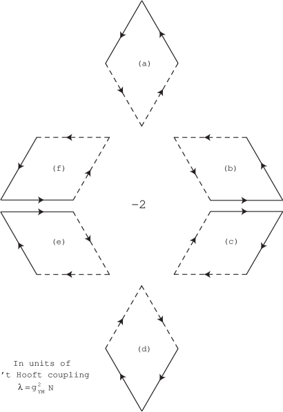
Figure 3: The basic “holomorphic” interaction plaquettes which enclose two units of lattice area. The solid lines correspond to fields, and the dashed lines to field derivatives. These are the terms appearing in $\mathfrak{D}_{1}^{h}$, and contribute with a coefficient of $-2$ (in units of $g^{2}_{YM}N$) to the amplitude. Notice that the bottom three are mirrors of the top three, flipped along the horizontal.

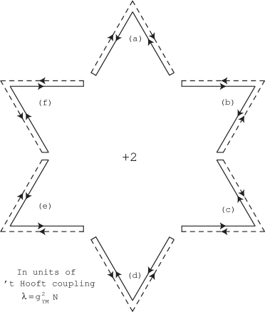
Figure 4: The basic “holomorphic” interaction plaquettes which enclose zero area. As before, the solid lines correspond to fields, and the dashed lines to field derivatives. These are the terms appearing in $\mathfrak{D}_{1}^{h}$, and contribute $+2$ (in units of $g^{2}_{YM}N$) to the amplitude. These terms are related individually to those in Figure 3 by commuting the derivative terms, as they appear in $\mathfrak{D}_{1}^{h}$. Again, the bottom three are mirrors of the top three, flipped along the horizontal.

In Figure 5 we show how the right-handed parallelogram plaquettes are related to the left-handed ones. Consider an operator of the form $tr(AB\Delta^{A}\Delta^{B})$ (plaquette (b) in Figure 3). Reading the trace in the opposite direction, we get $tr(BA\Delta^{B}\Delta^{A})$, transforming a right-handed operator into a left-handed one. These both arise from $\mathfrak{D}_{1}^{h}\sim Tr([A,B][\Delta^{A},\Delta^{B}])+\ldots$, which gives rise to a sum of terms of the form $tr(AB\Delta^{A}\Delta^{B})$ and $tr(BA\Delta^{B}\Delta^{A})$ at all lattice sites, and so the left-right handed flip arises from the commutation of $A,B$ and $\Delta^{A},\Delta^{B}$ in $\mathfrak{D}_{1}^{h}$.

Diagrammatically, this reversal corresponds to flipping the plaquette along the diagonal dividing the plaquette into two equilateral triangles, which are fundamental units of the lattice (this diagonal also separates the fields and the derivatives). Similarly, Figure 6 shows how the right-handed and left-handed corner plaquettes are related.

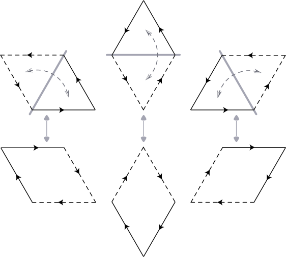
Figure 5: The diagrammatic relation between left-handed and right-handed open plaquettes.

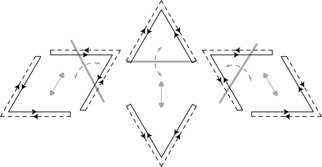
Figure 6: The diagrammatic relation between left-handed and right-handed corner plaquettes.

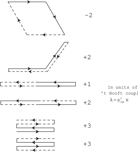
Figure 7: Examples of operators which mix holomorphic and anti-holomorphic fields. The open plaquette has the same weight as in Figure 3, and the corner plaquette has the same weight as in Figure 4. Due to some cancelations the third diagram has half the weight of a corner plaquette in Figure 4, while the fourth diagram carries the same weight as the corner plaquettes. The final two figures carry the weight $+3$. The numbers on the right side of the plaquettes shows their contributions in units of $g^{2}_{YM}N$.

Hermitian Conjugation of a plaquette simply reverses the direction in which the arrows flow. For example, conjugation of $tr(A\bar{C}\Delta^{A}\bar{\Delta}^{C})$ gives $tr(C\bar{A}\Delta^{C}\bar{\Delta}^{A})$, turning the original right-handed plaquette into a left-handed one. Each plaquette in $\mathfrak{D}_{1}^{h}$ is the conjugate of one plaquette in $\mathfrak{D}_{1}^{\bar{h}}$. The sum of $\mathfrak{D}_{1}^{h}$ and $\mathfrak{D}_{1}^{\bar{h}}$ is hermitian. Likewise, the first term in $\mathfrak{D}_{1}^{h\bar{h}}$ is hermitian and the sum of the second and third terms is also hermitian. Thus $\mathfrak{D}_{1}$ is hermitian with real eigenvalues, as expected, since it is the one-loop correction to the generator of the conformal group of the theory, and whose eigenvalues, giving the one-loop corrections to the scaling dimensions, must be real.

When expanding the sum in $\mathfrak{D}_{1}$, we have terms such as

$$\begin{split}\mathfrak{D}_{1}\>=\>-\>Tr\Big{(}&[A,B][\Delta^{A},\Delta^{B}]\>+\>[B,A][\Delta^{B},\Delta^{A}]\>+\>\\ &[A,B][\Delta^{B},\Delta^{A}]\>+\>[B,A][\Delta^{A},\Delta^{B}]\>+\>\ldots\Big{)}\end{split}$$ (3.8)

and after expanding the trace $Tr$ this gives rise to

$$\mathfrak{D}_{1}\>=\>-2\>tr\left(B_{i+3,j+2}A_{i+2,j+1}\Delta^{B}_{i+3,j+3}\Delta^{A}_{i+3,j+2}\>-\>B_{i+1,j+1}C_{i,j}\Delta^{C}_{i,j}\Delta^{B}_{i+1,j+1}\>+\>\ldots\right)$$ (3.9)

the trace is now over $U(N)$ generators. The factor of $2$ results from the equivalence of $[A,B][\Delta^{A},\Delta^{B}]$ and $[B,A][\Delta^{B},\Delta^{A}]$, both of which appear in the sum in $\mathfrak{D}_{1}$. The relative sign between the two terms displayed in (3.9) reflects the fact that they arise, respectively, from the first and second line of (3.8), which differ in their relative ordering of fields in the commutators.

To see how interaction plaquettes make their appearance, consider the operators

$$O_{1}\>=\>tr\left(\>A_{i+3,j}\>A_{i+3,j+1}\>A_{i+3,j+2}\>B_{i+3,j+3}\>B_{i+2,j+2}\>B_{i+1,j+1}\>C_{i,j}\>C_{i+1,j}\>C_{i+2,j}\right)$$ (3.10)

and

$$O_{2}\>=\>tr\left(\>A_{i+3,j}\>A_{i+3,j+1}\>B_{i+3,j+2}\>A_{i+2,j+1}\>B_{i+2,j+2}\>B_{i+1,j+1}\>C_{i,j}\>C_{i+1,j}\>C_{i+2,j}\right)$$ (3.11)

for some fixed $i,j$, and study the action of $\mathfrak{D}_{1}$ on $O_{1}$. We have

$$\mathfrak{D}_{1}\>O_{1}\>=\>2\>N\left(3O_{1}\>-\>O_{2}\>+\>\cdots\right)$$ (3.12)

with $\cdots$ representing other operators we are ignoring for now. Equation (3.12) also shows that a factor of $N$ arises from merging the traces in $\mathfrak{D}_{1}$ and $O_{1}$ ($O_{1}$ is a single trace operator), and the $3$ counts the number of corners in $O_{1}$, since the action of the dilatation operator is localized only at corners and straight parts of operators are not acted on by the dilatation operator. The factor of $N$ combines with the $g^{2}_{YM}$ in (3.1) to give the effective ’t Hooft coupling. Note that $\mathfrak{D}_{1}$ is one-loop planar dilatation operator.

Figures 9 and 8 depict equation (3.12) graphically. The general structure of interactions is as follows: each term in the expansion of $\mathfrak{D}_{1}$ can be represented diagrammatically as a plaquette. Such plaquettes can be inserted anywhere where the two dashed lines, which correspond to the derivatives in $\mathfrak{D}_{1}$, can be contracted with fields in an operator (the arrows on the fields and the derivatives with which they contract must run in opposite directions). The contracted fields disappear in the next time increment, to be replaced by the two remaining fields in the plaquette. The amplitude for such a transition is a numerical coefficient associated with the plaquette, and this defines the matrix element of the transfer matrix between these states. Of course there are in general many terms in the expansion of $\mathfrak{D}_{1}$ which have non-vanishing action when acting on a generic operator. Each such term gives rise to a possible transition, with the associated amplitude.

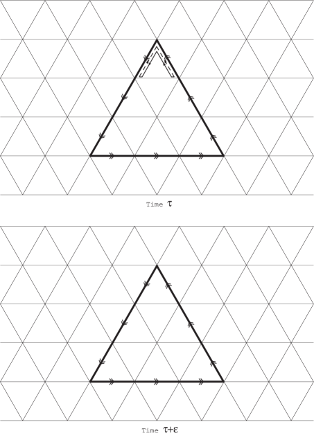
Figure 8: The action of a corner plaquette term at a corner in a single time step. This contributes +2 to the transition amplitude.

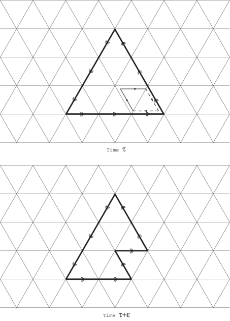
Figure 9: The action of an open plaquette term at a corner in a single time step. This contributes -2 in units of $g^{2}_{YM}N$ to the transition amplitude.

In general, every holomorphic or anti-holomorphic plaquette does one of two things: it either commutes two fields in the operator (adjusting the lattice indices appropriately), or leaves the order of the fields unchanged. This is obvious from the structure of the plaquettes.

The earlier argument that holomorphic operators form a closed subset can now be seen graphically. The only plaquettes which can contract into such operators must have two holomorphic derivatives (i.e.​ derivatives with respect to holomorphic fields), and as pointed out in Appendix A, these derivatives transform in the conjugate representation, for which the arrows run in the opposite direction. The two fields in the plaquette must then be holomorphic. As a result, the insertion of such a plaquette absorbs two holomorphic fields and replaces them with two holomorphic fields, and hence holomorphic operators transition to holomorphic operators. These considerations apply in an obvious fashion to anti-holomorphic operators as well. Plaquettes containing both holomorphic and anti-holomorphic fields also contain both holomorphic and anti-holomorphic derivatives, and their contraction with purely holomorphic or anti-holomorphic operators vanishes. These considerations also imply that mixed operators can never evolve to holomorphic or anti-holomorphic operators.

Recall also our definition of BPS operators. These are operators that are constructed solely from one of the three holomorphic (likewise anti-holomorphic) fields alone, and wrap the lattice any number of times more than zero, in a gauge-invariant way (they start and end at the same lattice site). The only plaquettes which could in principle be contracted with these operators must have two derivatives with respect to the same field, both holomorphic or anti-holomorphic, but not mixed. A glance back at equation (3.5) shows immediately that no such plaquettes exist, as $[\Delta^{A},\Delta^{A}]$, etc. vanishes identically. This justifies the term BPS we introduced earlier.

The evolution generated by the transfer matrix is (imaginary) time reversal symmetric, in the following sense: for any evolution from a string configuration associated to operator $O_{1}$ at time $\tau$ to configuration $O_{2}$ at time $\tau+\epsilon$ generated by a plaquette $p$, there exists a plaquette $\bar{p}$ that would transform configuration $O_{2}$ at time $\tau$ to $O_{1}$ at time $\tau+\epsilon$, or in other words, if we run time backwards, the string configuration $O_{2}$ at time $\tau+\epsilon$ is taken to configuration $O_{1}$ at time $\tau$ by the plaquette $\bar{p}$. The plaquette $\bar{p}$ which accomplishes this is gotten by flipping the plaquette $p$ along the diagonal as depicted in Figure 5 for zero area plaquettes, while for the closed plaquettes $p=\bar{p}$, as their action is proportional to the identity operator.

A more elaborate example of wave propagation is shown in Figure 10, with the configuration of the string depicted at four instants of time, and the plaquettes generating the transitions also displayed. Note that some of the plaquettes which appear in this example mix holomorphic and anti-holomorphic fields.

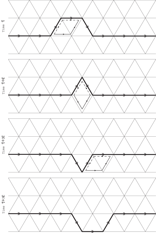
Figure 10: Following some possible string fluctuations for several time steps. This describes a wave propagating along the string.

It should be clear from this example that (planar level) fluctuations of strings can only take place at corners. In other words, the straight portions of strings can not be deformed. This behavior is clearly the reason BPS operators are protected.

The structure of the interaction plaquettes also make it evident that the string length is unchanged when it fluctuates. This is simply a restatement of the observation that the one-loop dilatation operator $\mathfrak{D}_{1}$ only connects operators of the same dimension, since for operators built only from the scalar bi-fundamental fields the dimension is the same as the length. (This generalizes in an obvious way to the fermion bi-fundamentals, if we take account of their canonical dimensions appropriately.) For the case of holomorphic or anti-holomorphic operators, this is also the statement of $R$-charge conservation, as noted previously.

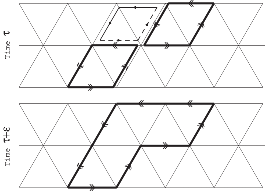
Figure 11: An example of a $1/N$ string interaction diagram, where a double trace operator merges with a single trace one. The $1/N$ suppression is appropriate to (bi)-fundamental fields.

4 Dynamical Pictures

In the previous section we discussed that how the gauge invariant operators of the ${\cal N}=1$, and in particular the holomorphic operators, can be realized on the two dimensional Moose diagram. We also outlined how to perform one-loop planar computations of two point functions, and hence anomalous dimension matrix, in a pictorial way, using the overlaps of operators on the lattice. In this section we build a closer connection with the spin chain on the Moose and/or the lattice theory picture.

4.1 Lattice Laplacian Picture

In section 3.2 we drew an analogy between the one-loop dilatation operator and the transfer matrix describing (Euclidean) time evolution. Wave propagation on a string is governed by a wave equation. We demonstrate here that a basis of operators can be chosen such that their time evolution is described by a Laplacian, together with extra contact terms, giving another perspective on the dynamics of the loops, and through our dictionary, the anomalous dimension matrix.

In this subsection we give a description of the string evolution in terms of solutions of a Laplace equation. First we must introduce a basis of operators. For concreteness, we focus on a subsector of operators $O_{i,j}$ of the form

$$O^{l}_{i,j}\>=\>tr\big{(}\>\overbrace{\underbrace{\overbrace{A\ \ \ldots\ \ A}^{i-1}\ \bar{C}\ A\ \ \ldots\ \ A}_{j-1}\ \bar{B}\ A\ \ \ldots\ \ A}^{p+2}\>\big{)}$$ (4.1)

with the operator $\bar{C}$ located in the $i$’th position, and the operator $\bar{B}$ located in the $j$’th. The superscript $l,\ l=1,2,\cdots,q$, denotes where (most of) the A’s line lies in the $q$ direction of the $2d$ lattice. In principle, the operators of the form (4.1) can have a “winding number”, counting the number of times the operator wraps the lattice. We focus on operators of winding number one, the generalization to higher winding modes goes through with the most obvious modifications. In $O^{l}_{ij}$ there are $i-1$ $A$’s appearing before $\bar{C}$ and $j-1$ before $\bar{B}$, but we do not assume that $\bar{C}$ appears before $\bar{B}$, so that both cases where $i<j$ and $i>j$ are allowed (but not $i=j$). The total length of operators of this form with winding number one is $p+1$, with $p$ the size of the lattice in the $A$ direction. Examples of such operators are depicted in Figure 12.

Figure 12: Examples of operators with winding number one, on a lattice of size $l=7$ in the $A$ direction, where we assume periodic boundary conditions at the edges. Both operators have length or dimension $d=l+1=8$. In the first case, $i=4,j=5$, so we denote it as $O_{4,5}$. In the second example $i=5,j=3$, so this operator is labeled $O_{5,3}$.

Recall that operators built strictly from $A$’s would be BPS, and would receive no anomalous dimension corrections. The presence of $\bar{B}$ and $\bar{C}$ causes this operator to no longer be BPS, but since fluctuations are allowed only to occur at corners and not along the straight portions of operators, this operator is in some sense almost-BPS in the large $p$ limit, as the portions of the operator away from the insertions of $\bar{B}$ and $\bar{C}$ remains BPS. These insertions are the $\mathcal{N}=1$ analogues of BMN-type impurities in the $\mathcal{N}=4$ theory.

An example of the evolution of such operators has already been shown in Figure 10, where the transitions are $O^{l}_{3,5}\rightarrow O^{l}_{4,5}\rightarrow O^{l}_{5,4}\rightarrow O^{l}_{6,4}$. As can readily be seen from Figure 10 and is inferred from discussions of previous section the dilatation operator $\mathfrak{D}_{1}$ does not act on the $l$ index and hence hereafter we drop the $l$ index and simply denote the operators of the form (4.1) by $O_{i,j}$.

For a general operator $O_{i,j}$ of the form (4.1) the action of the dilatation operator is given by

$$\mathfrak{D}_{1}\>O_{i,j}\>= +4\>O_{i,j}\>-\>O_{i-1,j}\>-\>O_{i+1,j}\>-\>O_{i,j-1}\>-\>O_{i,j+1}$$ (4.2)

$$+\delta_{i+1,j}\left(O_{i,j-1}+O_{i+1,j}-O_{i,j}-O_{i+1,j-1}\right)$$

$$+\delta_{i-1,j}\left(O_{i,j+1}+O_{i-1,j}-O_{i,j}-O_{i-1,j+1}\right)$$

with the constant $4$ on right-hand side counting the number of corners in the operator. The second line is a contact term which takes account of the configuration where the two impurities sit next to each other. The $O_{i,j}$ in the contact term correct the number of corners and the last term accounts for the flip transitions when a bump pointing up transitions to a bump pointing down and vice-versa.

We would now like to show the appearance of a latticized Laplacian. To facilitate the rewriting, we introduce the forward and backward shift operators acting the first or second index

$$\begin{split}\mathbb{S}_{i}\>O_{i,j}\>=\>O_{i+1,j}\ ,\ \ \ \ \ \ \ \ \ \ \ \ \hat{\mathbb{S}}_{i}\>O_{i,j}\>=\>O_{i-1,j}\ ,\\ \mathbb{S}_{j}\>O_{i,j}\>=\>O_{i,j+1}\ ,\ \ \ \ \ \ \ \ \ \ \ \ \hat{\mathbb{S}}_{j}\>O_{i,j}\>=\>O_{i,j-1}\ ,\end{split}$$ (4.3)

and the identity operator

$$\mathds{1}\>O_{i,j}\>=\>O_{i,j}\ .$$ (4.4)

In terms of these we define the forward and backward difference operators

$$\begin{split}\nabla_{i}\>\>\equiv\>\mathbb{S}_{i}\>-\>\mathds{1}\\ \hat{\nabla}_{i}\>\>\equiv\>\mathds{1}\>-\>\hat{\mathbb{S}}_{i}\\ \nabla_{j}\>\>\equiv\>\mathbb{S}_{j}\>-\>\mathds{1}\\ \hat{\nabla}_{j}\>\>\equiv\>\mathds{1}\>-\>\hat{\mathbb{S}}_{j}\end{split}$$ (4.5)

from which we also define two Laplacian operators acting on $i,j$

$$\begin{split}\nabla^{2}_{i}\>\equiv\>\nabla_{i}\>-\>\hat{\nabla}_{i}\\ \nabla^{2}_{j}\>\equiv\>\nabla_{j}\>-\>\hat{\nabla}_{j}\end{split}$$ (4.6)

and the total Laplacian

$$\nabla^{2}_{i,j}\>\equiv\>\nabla^{2}_{i}\>+\>\nabla^{2}_{j}$$ (4.7)

With these definitions, we can rewrite the dilatation operator, when acting on the almost-BPS operators (4.2) as

$$\mathfrak{D}_{1}\>O_{i,j}\>=\>\Big{(}\nabla^{2}_{i,j}\>-\>\delta_{i+1,j}\nabla_{i}\>\hat{\nabla}_{j}\>-\>\delta_{i-1,j}\hat{\nabla}_{i}\>\nabla_{j}\Big{)}O_{i,j}$$ (4.8)

The second and third term above are contact terms which correct for the case when we have a minimal size bump, in which case a bump pointing up can flip to a bump pointing down and vice-versa, and also the fact that for minimal size bumps there are only three corners instead of four.

In writing the action of the dilatation operator in this form, we have made evident the picture of operator evolution in terms of waves propagating on a fluctuating string manifest.

To find the eigenvalues and eigenstates of $\mathfrak{D}_{1}$ let us focus on (4.2). The cyclicity of the trace in (4.1) is the remnant of the translational invariance of the lattice in the $A$ direction. This implies that the eigenstates of (4.2) should only be a function of $i-j$. Defining $k\equiv i-j$ (note that the $k$ index does not take the value 0) then (4.2) takes the form

$$\begin{split}\mathfrak{D}_{1}O_{k}&=4O_{k}-2(O_{k-1}+O_{k+1})\ ,\ \ \ \ k\neq\pm 1\\ \mathfrak{D}_{1}O_{+1}&=3O_{+1}-2O_{+2}-O_{-1}\\ \mathfrak{D}_{1}O_{-1}&=3O_{-1}-2O_{-2}-O_{+1}\end{split}$$ (4.9)

Next, let us define

$$O^{\pm}_{k}=O_{k}\pm O_{-k}\ .$$ (4.10)

In terms of $O^{\pm}_{k}$ (4.9) the equations for $O^{+}$ and $O^{-}$ decouple:

$$\mathfrak{D}_{1}O^{\pm}_{k} =4O^{\pm}_{k}-2(O^{\pm}_{k-1}+O^{\pm}_{k+1})\ ,\ \ \ k\neq\pm 1\ ,$$ (4.11a)

$$\mathfrak{D}_{1}O^{+}_{1} =2(O^{+}_{1}-O^{+}_{2})\ ,$$ (4.11b)

$$\mathfrak{D}_{1}O^{-}_{1} =4O^{-}_{1}-2O^{-}_{2}\ .$$ (4.11c)

If we define

$$O^{+}_{0}\equiv O^{+}_{1}\ ,\ \ O^{-}_{0}\equiv 0\ ,$$ (4.12)

then equations (4.11b,c) become compatible with (4.11a) once we relax the $k\neq\pm 1$ condition and allow $k$ to also take the value 0. In fact (4.12) plays the role of “boundary conditions” for the Laplace equation of motion for $O^{\pm}_{k}$’s, $k\geq 0$; $O^{+}_{k}$ have a Neumann boundary condition and $O^{-}_{k}$ Dirichlet. We should stress that this “boundary condition” is not related to the boundary conditions for the closed strings, which still have periodic boundary conditions. Therefore,

$$Q^{+}_{n} \>=\>\sum_{k=1}^{p+1}O^{+}_{k}\cos(\frac{2\pi\ nk}{p+1})\ ,$$ (4.13a)

$$Q^{-}_{n} \>=\>\sum_{k=1}^{p+1}O^{-}_{k}\sin(\frac{2\pi\ nk}{p+1})\ ,$$ (4.13b)

and both have $\mathfrak{D}_{1}$ eigenvalues

$$\omega^{\pm}_{n}\>=\>\frac{g^{2}_{YM}N}{(2\pi)^{2}}\left(1-\cos(\frac{2\pi n}{p+1})\right)\ ,$$ (4.14)

where we have reintroduced the ’t Hooft coupling $\lambda=g^{2}_{YM}N/(4\pi)^{2}$.

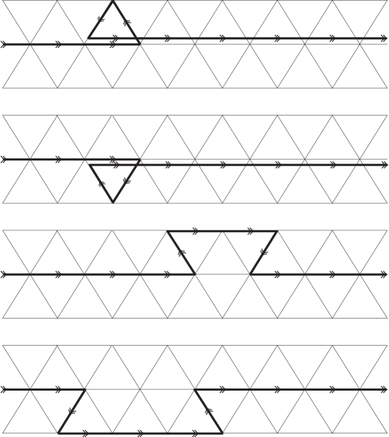
Figure 13: Examples of operators with winding number one, on a lattice of size $l=7$ in the $A$ direction, where we assume periodic boundary conditions at the edges. Both operators have length or dimension $d=l+1=8$. In the first case, $i=4,j=5$, so we denote it as $O_{4,5}$. In the second example $i=5,j=3$, so this operator is labeled $O_{5,3}$.

One could repeat a similar analysis with operators of the form

$$\hat{O}^{k}_{i,j}\>=\>tr\left(B_{i,j}A^{k}CA^{p-k+1}\right)\ ,$$ (4.15)

which are in the holomorphic sector. For these operators we again find a result similar to the previous non-holomorphic two impurity case. An example of such operators and their time evolution is depicted in Figure 13.

4.2 The BMN Limit

It is instructive to consider the “BMN” limit of our ${\cal N}=1$ theory and its realization on the two dimensional triangle lattice. As this point has to some extent been discussed in the literature, especially on the gravity side and when taking the Penrose limit, we will be very brief and only address some issues related to the the gauge theory. For some earlier works on the Penrose limit of orbifolds, see [29, 30, 32, 33].

Let us consider the $p=q$ case. The BMN-type limit is then taking $p,N\to\infty$ while keeping $g^{2}_{YM}$ and $p^{2}/N$ fixed. This BMN-type limit can be thought of as the continuum limit over the discretized string worldsheet. Restricting to operators made out of the bi-fundamental scalars, this is in fact also the continuum limit over a 2+1 dimensional target space. The BMN-type operators are those with dimension (or $R$-charge) of order of $p$. The BMN vacuum states are the straight lines wrapping the lattice. These operators may be in the $A$, $B$ or $C$ directions and in the twisted or untwisted sector, e.g. $tr(A_{i,j+1}A_{i,j+2}\cdots A_{i,j+p})\ ,\ i=1,2,\cdots,p$. As discussed earlier, these operators are BPS and have vanishing anomalous dimension and are labeled by two quantum numbers: their dimension (or $R$-charge) $p$ and the $i$ index (or its Fourier transform). Moreover, there is another possibility that this operator wraps the lattice in the $A$ direction some number of times. This “winding” $w$ is hence the third quantum number needed to specify the vacuum state. (The dimension of the operator is then $pw$.)

From the dual string theory viewpoint, this operator is the vacuum state for the discrete light-cone quantization (DLCQ) of string theory on the corresponding plane-wave [30]. The string can only move freely in one direction (other than the light-cone direction) and is confined in the other directions due to the harmonic oscillator potential coming from the background plane-wave. Therefore, the vacuum state is only labeled by three quantum numbers, $p^{+}$, the light-cone winding $w$, and a momentum which is the Fourier transform of the $i$ index.

The string excitations above the vacuum are then given by placing small bumps on this straight line of $A$’s (as depicted in Figure 10). In the large $p$ limit these are almost BPS BMN-type operators.

One may read off the effective ’t Hooft coupling for this case from (4.14). The result of computations, when $p=q$, are

$$\lambda^{\prime}=\frac{g^{2}_{YM}N}{p^{2}}\$$ (4.16)

where $\lambda^{\prime}$ is the effective dressed ’t Hooft coupling. This result may be argued for by noting that the ${\cal N}=1$ theory we are considering is obtained as a $\mathbb{Z}_{p}\times\mathbb{Z}_{p}$ orbifold of a $U(Np^{2})$ ${\cal N}=4$ gauge theory for which the effective ’t Hooft coupling in the BMN sector with $R$-charge $J$ is $\lambda^{\prime}=\frac{(g_{YM}^{parent})^{2}(Np^{2})}{J^{2}}$. In our case $J=p$ and $g^{2}_{YM}$ and $(g_{YM}^{parent})^{2}$ are related as in (2.4). Note that this argument is only applicable to the untwisted sector. However, as in the usual string theory, one expects this to be valid for the twisted sector as well. This expectation is indeed confirmed by explicit computations we have shown in section 4.1.

4.3 Spin Chain Picture and Integrability

In (Lorentzian) real space, the path integral gives the amplitude for a configuration of the system at some initial time to evolve to the prescribed configuration at the final time. It involves summing over all allowed intermediate states with a given weight, which is the exponential of minus $i$ times the action. When going over to Euclidean space, $i$ times the action becomes minus the Euclidean action, which is just the energy. So in Euclidean space the path integral for a $d+1$ dimensional system is really the partition function of a classical $d+1$ dimensional statistical mechanics system. Using the transfer matrix, this can be related to a quantum mechanical system in $d$ dimensions. This involves taking a limit of the transfer matrix formulation in which the time variable becomes continuous, tuning the spatial and temporal couplings in a special way [34].

We have a Euclidean system in which a configuration of strings on a two-dimensional lattice evolves to another configuration on the same two-dimensional lattice in a discrete Euclidean time step. We have already described how to compute the amplitude for such a transition, which is given by the matrix elements of the transfer matrix between the appropriate initial and final configurations. As we discussed previously, the dimensionality of the transfer matrix is determined by the number of allowed possible string configurations on the lattice. We would now like to relate this to a lower dimensional quantum mechanical system. As usual, in the limit of infinitesimal time steps, the transfer matrix can be expanded as

$$\hat{T}\>=\>1\>-\>\epsilon\hat{H}$$ (4.17)

with $\epsilon$ the infinitesimal time step. By analogy to the relationship between the classical two-dimensional Ising model and the quantum one-dimensional Ising chain, we expect the quantum Hamiltonian to describe a two-dimensional system. Such a description will be briefly discussed in section 6.1, where we will see that the description can be given in terms of a 2+1-dimensional Euclideanized Lattice gauge theory in a temporal gauge, in the conformal fixed point.

However, because the natural description we have been using for the state of the system at a given time is in terms of string configurations, instead of the configuration of all link variables on a slice, the lower dimensional system will naturally turn out to describe $(1+1)$-dimensional objects.

Again, as is the usual structure, in the infinitesimal time limit, only transitions which involve zero or one “flip” contribute at first order in $\epsilon$. The flips occur when a single insertion of the plaquettes in Figure 3 flip two legs of a triangle along a diagonal. Zero flips are due to the insertions of plaquette terms in Figure 4. Earlier we identified the matrix elements of the transfer matrix for a transition between initial and final states with the matrix elements of the one-loop dilatation operator. If we identify $\epsilon$ with the coupling (up to a numerical factor arising from the commutator structure of (3.5)) $2\lambda/(4\pi)^{2}$, where $\lambda=g_{YM}^{2}N$ is the ’t Hooft coupling, then the fact that only zero or single flip transitions contribute is a consequence of keeping only one-loop contributions to the dilatation operator, i.e. ​ weak ’t Hooft coupling. So we make this identification, together with a slight modification of our earlier construction of the transfer matrix, where we now identify the transfer matrix with the complete dilatation operator to one-loop, including both the tree level and the one-loop contributions (3.1). Inclusion of the tree-level classical dimensions allows us to extract the identity term in (4.17).

A string loop is formed from a series of links, labeled $L_{i}$, for $i=1,\ldots,d$, with $d$ the total length of the loop. The state of each link is described by a basis vector in a vector space $\mathds{V}$. For a general operator, $\mathds{V}$ is a six-dimensional vector space with basis vectors corresponding to the fields $A,B,C,\bar{A},\bar{B},\bar{C}$ and hence the Hilbert space of a loop of length $d$ is $6^{d}$ dimensional. The basis for $\mathds{V}$ can be decomposed into $\bf{3}\oplus\bar{\bf{3}}$ of $SU(3)$. This $SU(3)$ is the subgroup of the $SU(4)_{R}$ of the ${\cal N}=4$ parent gauge theory before the orbifolding.

When restricting to holomorphic operators, we work in a three-dimensional complex subspace of this vector space which transform in ${\bf 3}$ or ${\bar{\bf 3}}$ of $SU(3)$. In the holomorphic sector $\mathds{V}$ reduces to $\mathbb{C}^{3}$. We denote the basis vectors for the $i$’th link as $\hat{e}_{i}^{\alpha}$, where $\alpha$ ranges over $A,B,C,\bar{A},\bar{B},\bar{C}$. We denote the state of the $i$’th link as $\hat{s}_{i}$. We introduce for later use the permutation operator

$$\hat{P}_{i,i+1}\ \hat{s}_{i}\otimes\hat{s}_{i+1}\>\equiv\>\hat{s}_{i+1}\otimes\hat{s}_{i}\ ,$$ (4.18)

This operator acts on tensor products of vector spaces associated to neighboring links, or alternatively on pairs of nearest neighbor links, and acts on the states at the positions $i$ and $i+1$ by exchanging them. The full Hilbert space $\mathcal{H}$ of the string is the tensor product over the Hilbert spaces of each individual link

$$\mathcal{H}\>=\>\bigotimes_{i=1}^{d}\mathcal{H}_{i}\ .$$ (4.19)

Identify the matrix element of the transition matrix between states $O_{i}$ and $O_{j}$ as

$$T_{i,j}\>=\>\big{<}\>\mathcal{O}_{i}\>|\>\hat{T}\>|\>\mathcal{O}_{j}\>\big{>}\>=\>\big{<}\>\mathcal{O}_{i}\>|\left({\mathfrak{D}}_{0}\>+\>\frac{g_{YM}^{2}}{(4\pi)^{2}}{\mathfrak{D}}_{1}\right)|\>\mathcal{O}_{j}\>\big{>}\ .$$ (4.20)

Normalize operators so that

$$\big{<}\>\mathcal{O}_{i}\>|\>\mathcal{O}_{j}\>\big{>}\>=\>\frac{1}{d}\delta_{ij}\ ,$$ (4.21)

with $d$ the classical dimension of the operator. Then,

$$\big{<}\>\mathcal{O}_{i}\>|\>{\mathfrak{D}}_{0}\>|\>\mathcal{O}_{j}\>\big{>}\>=\>\delta_{i,j}\ .$$ (4.22)

With this normalization (4.20) and (3.7) are equal. Since the operators with different classical dimension have zero overlaps, in first and all higher loops and even at non-planar level, $\mathcal{H}$ is the Hilbert space for $T$ and the set of all the operators on the $2d$ lattice can be classified into operators of given classical dimension. Moreover, for the same reason (4.22) is an appropriate normalization. If $i=j$, then ${\mathfrak{D}}_{1}$ equals twice the number of corners in $O_{i}$ and if $i\neq j$, then ${\mathfrak{D}}_{1}$ equals zero if the two operators cannot be connected by a single plaquette, and equals minus two if they can.

Hereafter we only consider the holomorphic sector. Noting the planar behavior of the transfer matrix when acting on the strings in the holomorphic sector, it can be written in the following form

$$\hat{T}\>=\>\sum_{i=1}^{d}\left(1\>+\>\frac{2g_{YM}^{2}N}{(4\pi)^{2}}\sum_{\alpha,\beta}\sum_{\delta,\rho}\ C_{\beta\rho}^{\alpha\delta}\ T_{i+1}^{\dagger\alpha}T_{i+1}^{\beta}T_{i}^{\dagger\delta}T_{i}^{\rho}\right)\ .$$ (4.23)

The indices $\alpha,\beta,\gamma,\delta$ label the states and range over $A,B,C$ for the holomorphic subsector. Here the $T_{i}^{\dagger\alpha}$ is a creation operator acting in the Hilbert space associated with the $i$’th link, producing the state indexed by $\alpha$. Likewise, $T_{i}^{\beta}$ is an annihilation operator for the state indexed by $\beta$. This form follows from requiring that the transfer matrix as an operator generates the matrix elements via (4.20). The matrix $C_{\beta\rho}^{\alpha\delta}$ has value

$$C_{\beta\rho}^{\alpha\delta}\>=\>\left(\delta_{\beta}^{\alpha}\delta_{\rho}^{\delta}-\delta_{\rho}^{\alpha}\delta_{\beta}^{\delta}\right)\ ,$$ (4.24)

and the following symmetry

$$C_{\beta\rho}^{\alpha\delta}\>=\>C_{\rho\beta}^{\delta\alpha}\ .$$ (4.25)

Note that these are in fact the spin operators which will appear again below.

To see how the spin chain structure arises, it is useful to consider an example. Take the set of operators

$$\begin{split}O_{1}=Tr(AABBCC)\ ,\\ O_{2}=Tr(ABABCC)\ ,\\ O_{3}=Tr(AABCBC)\ ,\\ O_{4}=Tr(CABBCA)\ ,\end{split}$$ (4.26)

which form a closed set under renormalization at one-loop planar level. Consider now some matrix elements of the transfer matrix (4.20) between these states

$$T_{1,1}\>=\>1\>+\>2\frac{g_{YM}^{2}N}{(4\pi)^{2}}\ \frac{\mathscr{C}}{d}$$ (4.27)

where $\mathscr{C}$ is the number of corners in the operator $\mathcal{O}_{1}$ (three in this example). We also have

$$T_{2,1}\>=\>-2\frac{g_{YM}^{2}N}{(4\pi)^{2}}\frac{1}{d}$$ (4.28)

We expand the transfer matrix to first order, using (4.17), to find the Hamiltonian

$$\big{<}\>\mathcal{O}_{1}|\>\hat{T}\>|\mathcal{O}_{1}\>\big{>}\>=\>1\>-\>\epsilon\>\big{<}\>\mathcal{O}_{1}|\>\hat{H}\>|\mathcal{O}_{1}\>\big{>}$$ (4.29)

and

$$\big{<}\>\mathcal{O}_{2}|\>\hat{T}\>|\mathcal{O}_{1}\>\big{>}\>=\>-\>\epsilon\>\big{<}\>\mathcal{O}_{2}|\>\hat{H}\>|\mathcal{O}_{1}\>\big{>}$$ (4.30)

Setting $\epsilon=\frac{2g_{YM}^{2}N}{(4\pi)^{2}}$, allows us to identify the Hamiltonian $\hat{H}$ as

$$\hat{H}\>=\>\sum_{i=1}^{d}\>\left(1\>-\>\hat{P}_{i,i+1}\right)$$ (4.31)

where $\hat{P}_{i,i+1}$ is the permutation operator, the identity is understood to act on the tensor product of two vector spaces, and we have periodically identified the boundaries. Note that the infinitesimal time limit corresponds to small ’t Hooft coupling, where the perturbative expansion of the dilatation operator (3.1) is valid. In making this identification, we have made use of the observation that the number of corners in a loop equals the classical dimension minus the number of straight pieces in the loop. In general the number of corners is not a conserved quantity, so the other operators with which a given operator can mix may contain different numbers of corners, but it is generically true (for holomorphic operators and at planar level) that the number of corners fixes the number of other operators with which mixing occurs.

The Hamiltonian (4.31) is the Hamiltonian of an integrable (anti-ferromagnet) $SU(3)$ spin chain [8, 27, 28]. The integrability of the (anti-)ferromagnetic $SU(N)$ spin chain, construction of the Lax pairs and transfer matrix and the infinite number of commuting conserved charges in terms of the Lax pairs has been done in [39] and may also be found in the Appendix A of [27]. Moreover, using the algebraic Bethe ansatz equations eigenvalues of the Hamiltonian has been given in terms of the rapidity parameter of the Bethe ansatz [39]. Therefore, here we do not repeat the integrability arguments.

A nice representation of the permutation operator (4.18) and hence the spin chain Hamiltonian (4.31) can be given as follows: since the state at each link is a vector in the complex vector space $\mathds{V}$ of dimension six, we can introduce, by analogy to the spinors, the spin operator acting on $\mathds{V}$, with the representation

$$S^{ab}_{ij}\>=\>\delta^{a}_{i}\>\delta^{b}_{j}\>-\>\delta^{a}_{j}\delta^{b}_{i}$$ (4.32)

with $(a,b)$ ranging from $1,\ldots,6$, and the indices $(i,j)$ being the matrix indices for this six-dimensional representation. Restricting ourselves to holomorphic operators, we can project to the complex three-dimensional subspace of $\mathds{V}$ spanned by $A,B,C$. Taking a three-dimensional representation of the spin operators (4.32), we can rewrite the Hamiltonian as

$$\hat{H}\>=\>2\>+\>\frac{1}{2}\left(S^{ab}_{l}S^{ab}_{l+1}\right)\>-\>\frac{1}{4}\left(S^{ab}_{l}S^{ab}_{l+1}\right)^{2}\ .$$ (4.33)

This is the Hamiltonian for an integrable $SU(3)$ spin chain [39, 40, 27]. It is important to point out that the counting we have presented is particular to the case of holomorphic operators; the additional complication with non-holomorphic operators can be traced to the weights appearing in Figure 7.

So far we have shown, basically by construction, that the Hamiltonian of a spin chain system with certain nearest neighbor interactions is equivalent to the one-loop planar dilatation operator of the ${\cal N}=1$ quiver gauge theory in the sector with operators made only out of three kinds of bi-fundamental scalars. As discussed, the equivalence is most simply seen and established in the basis where we label our states by the oriented closed loops on the two dimensional lattice.

One may try to rephrase the above statement in the language of the path integral and partition functions of the two sides. The partition function of the two dimensional statistical mechanical system, with ${\cal O}_{i}$ and ${\cal O}_{f}$ as the initial and final states, is defined as

$$\begin{split}Z_{{\rm spin\ chain}}[\beta;{\cal O}_{i},{\cal O}_{f}]&=\langle{\cal O}_{f}|e^{\beta\hat{H}}|{\cal O}_{i}\rangle\cr&=\sum_{\{\mathcal{O}_{j_{1}}\}}\cdots\sum_{\{\mathcal{O}_{j_{M}}\}}\langle\mathcal{O}_{f}|\hat{T}|\mathcal{O}_{j_{1}}\rangle\langle\mathcal{O}_{j_{1}}|\cdots|\mathcal{O}_{j_{M}}\rangle\langle\mathcal{O}_{j_{M}}|\hat{T}|\mathcal{O}_{i}\rangle\ ,\end{split}$$ (4.34)

where $\{\mathcal{O}_{j_{k}}\}$ denote the set of all closed loops on the lattice. We should also take $M\to\infty$ at the end of the computation. Each sum over $\{\mathcal{O}_{j_{k}}\}$ can in turn be decomposed into sums over sets containing operators of definite classical dimension.

On the other hand, in the ${\cal N}=1$ SYM, if we restrict ourselves to insertions of operators consisting only of scalars, then the transition amplitude between the initial and final states ${\cal O}_{i}$ and ${\cal O}_{f}$ is

$$\begin{split}Z_{2d\ {\rm reduced\ SYM}}[g^{2}_{YM}N;{\cal O}_{i},{\cal O}_{f}]&=\int[D\Phi]\ e^{-S_{reduced}}\ {\cal O}_{i}\ {\cal O}_{f}\cr&=\sum_{\{gauge\ inv.\ opt.\}}\langle{\cal O}_{f}|e^{-{\mathfrak{D}}}|{\cal O}_{i}\rangle\ ,\end{split}$$ (4.35)

where the subscript reduced stands for the reduction to a sector of scalars and the gauge invariant operators in this sector are identified with the orientable closed loops on the lattice, owing to the block diagonal nature of the transfer matrix (or equivalently $\mathfrak{D}_{1}^{h}$) described above.

It is interesting to see if the above correspondence between the 2+1 dimensional spin chain and the holomorphic sector (or more generally the sector made out of scalars) of the ${\cal N}=1$ SYM theory can be extended beyond this sector to also include the gauge fields. In sections 5 and 6.2 we will argue that this may be achieved if we view the 2+1 theory to as part of a 3+(2+1) six-dimensional theory.

5 Relation to AdS/CFT and Brane Box Models

As discussed earlier, the ${\cal N}=1$ $U(N)^{pq}$ gauge theory of interest can be obtained from an ${\cal N}=4$ $U(Npq)$ SYM theory, via a specific $\mathbb{Z}_{p}\times\mathbb{Z}_{q}$ orbifolding. The action of this orbifold on the scalars appears as a non-trivial $U(Npq)$ gauge rotation (which is not in a subgroup of $U(N)^{pq}$) while for the gauge fields there is no such twist.

The above orbifolding can also be understood from the gravity (string theory) dual to the $U(Npq)$ ${\cal N}=4$ SYM. The gravity dual background in this case is $AdS_{5}\times S^{5}$ with $R_{S^{5}}^{4}=l_{s}^{4}g_{s}Npq$. The orbifolding is then acting on the $S^{5}$ part. To see this, consider the $S^{5}$ embedded in a $\mathbb{C}^{3}$ as $\sum_{i}z_{i}^{2}=R^{2}$. The action of $\mathbb{Z}_{p}\times\mathbb{Z}_{q}$ on $z_{i}$ is

$$\mathbb{Z}_{p}:\left\{\begin{array}[]{ccc}z_{1}\equiv e^{\frac{2\pi i}{p}}z_{1}\\ \\ z_{2}\equiv e^{-\frac{2\pi i}{p}}z_{2}\end{array}\right.\mathbb{Z}_{q}:\left\{\begin{array}[]{ccc}z_{1}\equiv e^{\frac{2\pi i}{q}}z_{1}\\ \\ z_{3}\equiv e^{-\frac{2\pi i}{q}}z_{3}\end{array}\right.$$ (5.1)

The $AdS_{5}\times S^{5}/\mathbb{Z}_{p}\times\mathbb{Z}_{q}$ space can also be obtained as the near horizon geometry of a stack of $N$ D3-branes probing a $\mathbb{C}^{3}/\mathbb{Z}_{p}\times\mathbb{Z}_{q}$ singularity, where the branes are sitting at the $z_{i}=0$ fixed point. From this brane setup it is evident that the dual theory should be a $U(N)^{pq}$ gauge theory with bi-fundamental matter fields, as the $z_{i}=0$ is the point where the stack of branes and their orbifold images are coincident. The brane setup also sheds light on (2.4), recalling the notion of fractional branes [35] and the fact that the RR-charge (or effective tension) of the branes at the orbifold is $\frac{1}{l_{s}^{4}g_{s}}\cdot\frac{1}{pq}$ and that the tension, which is the coefficient in front of the Born-Infeld action for the brane, is (the inverse square of) the coupling for the low energy Yang-Mills theory living on the brane. Moving the branes away from the orbifold fixed point corresponds to moving to the Higgsed phase (Coulomb branch) of the $U(N)^{pq}$ theory [35] where the conformal symmetry is also broken. We will come back to this point in the next section. One may also try to take the Penrose limit(s) on the $AdS_{5}\times S^{5}$ geometries; this has been carried out for example in [30].

The two dimensional lattice is most easily seen in the T-dual picture of the above orbifold scenario. Let us denote the angular parts of $z_{1}/z_{2}$ and $z_{1}/z_{3}$ by $\alpha$ and $\beta$. These are the two $S^{1}$ directions where the orbifolding acts. Now, perform two T-dualities on the $\alpha$ and $\beta$ directions. The stack of $N$ D3-branes is mapped to $N$ D5-branes. The metric of the $\mathbb{C}^{3}/\mathbb{Z}_{p}\times\mathbb{Z}_{q}$ has off-diagonal pieces once two of the coordinates are chosen along the $\alpha$ and $\beta$ directions. These off-diagonal terms upon T-duality become NSNS $B$-fields whose three-form flux, in the near horizon geometry we are interested in, corresponds to intersecting smeared NS5-branes. The above can be summarized in the following simplified five-brane setup: Consider a stack of $N$ D5-branes along the 012345 directions and two sets of $p$ (and $q$) NS5-branes along the 012346 (and 012357) directions. The NS5-branes are respectively smeared in the 4 and 5 directions, and the D5-branes are localized in the 6789 directions. The 45 plane is covered by the $\alpha$ and $\beta$ directions mentioned earlier and is wrapping a two torus. The $\alpha$ and $\beta$ directions do not form an orthogonal basis for this torus.

The above intersecting brane setup leads to a generalization of the Hanany-Witten type brane configuration [37], where the D5-branes now have a finite extent in two directions. This forms the brane box picture [38, 41, 31, 42, 43, 44]. In our brane setup obtained from T-duality, however, the NS5-branes are smeared while in the brane box models all the fivebranes are localized. Nevertheless this does not affect the main picture or the fact that we are dealing with a (3+1 dimensional) conformal field theory.

The brane setup of the brane box model is as follows [38, 31]:

$\bullet$ $N$ D5-branes along 012345.

$\bullet$ $p$ NS5-branes along 012346, and uniformly distributed on the $x^{5}$ direction.

$\bullet$ $q$ NS5-branes along 012357, and uniformly distributed along the $x^{4}$ direction.
The $x^{4}$ and $x^{5}$ directions are periodically identified with radii $R_{4}$ and $R_{5}$. The 45 plane is then like a two dimensional lattice with $p\times q$ sites. The size of the unit cell on the lattice is $\frac{R_{4}R_{5}}{pq}$.

The low energy effective theory living on the above intersecting brane setup is a 3+1 dimensional $U(N)^{pq}$ gauge theory with $A,B$ and $C$ bi-fundamentals corresponding to open strings stretched between segments of the D5-branes, i.e. they are the links on the lattice, exactly as explained earlier. The intersecting brane system is 1/8 BPS and preserves 4 supercharges; therefore, the low energy effective theory is an ${\cal N}=1$ SYM theory. The rotation in the $89$ plane then corresponds to the $U(1)$ $R$-symmetry of the theory. The couplings of all the $pq$ $U(N)$ factors are equal, as we have chosen a uniform distribution of NS5-branes. This coupling is equal to the coupling of the $5+1$ dimensional $U(N)$ SYM on the $N$ D5-branes divided by the volume of each cell: $g^{2}_{5+1\ YM}\times\frac{pq}{R_{4}R_{5}}=g^{2}_{3+1\ YM}\ pq$; $g^{2}_{3+1\ YM}=g_{s}$ [38]. This is another way of stating eq.(2.4). We see that the explicit dependence on the size of the torus, or the lattice spacing, drops out; this is a sign of the conformal symmetry at the level of the $3+1$ dimensional theory. As a result, the lattice spacing remains an arbitrary parameter. The superpotential of this model, which has a natural appearance on the $2d$ oriented triangle lattice (cf. (2.5)) may also be read from the brane setup [31].

The brane box model provides a more geometric view of the $2+1$ dimensional (conformal) lattice we have developed in previous sections. Moreover, it makes closer contact with string theory. In this setup one may interpret the $2+1$ latticized string theory as a discretized version of a specific sector of the ${\cal N}=(1,1)$ little string theory living on the type IIB fivebranes. From this viewpoint, the time direction on the lattice theory is identified with the time direction along the branes. The brane box model also suggests that if we include the site variables, i.e. the vector multiplets of the $3+1$ dimensional ${\cal N}=1$ theory, we should obtain a six dimensional string theory with two directions on a fuzzy two-torus.

6 Higgsed Phase

So far we have studied the ${\cal N}=1$ gauge theory at its conformal fixed point (line). This corresponds to the case where the bi-fundamentals have zero VEV. It is possible to give a non-zero VEV to $A$’s, $B$’s and $C$’s in a such a way that we preserve the supersymmetry and hence the $U(1)$ R-symmetry. This would, however, break the conformal symmetry. From the gravity viewpoint discussed in the previous section this corresponds to taking the stack of $N$ D3-branes away from the orbifold fixed point. From the two dimensional lattice point of view, however, this corresponds to introducing a specific length scale on the two dimensional lattice. In other words, the spacing of the lattice now depends on the VEV’s.

In this section we consider such Higgsing and study the special case that all of the $3pq$ bi-fundamentals acquire non-zero, but equal VEV’s. First we check that this leads to a $2+1$ dimensional effective $U(N)$ lattice gauge theory, now with fixed lattice spacing and next discuss its connection to deconstruction [47].

6.1 Lattice Gauge Theory Picture

What we have is a three-dimensional Euclidean lattice gauge theory in a temporal gauge where the timelike links have had their field values set to zero. This is a discretized Hamiltonian lattice gauge theory. The lattice action of this system is just the plaquette action we have already presented. The operators we have been discussing are literally Wilson loops in this picture. A three dimensional lattice gauge theory has two fixed points: the IR fixed point a UV fixed point. The UV fixed point is a trivial fixed point about which the theory is free. The IR fixed point is a non-trivial one at which the theory flows to an interacting three dimensional conformal field theory. In the IR our lattice gauge theory obviously would look like a continuum theory as we cannot probe the discreteness of the lattice. In fact, one should be more careful, because we are working on a torus. The above then becomes exact only for large $p,q$.

Our viewpoint then provides a relation between the transfer matrix already presented and a three-dimensional Euclidean lattice gauge theory. We take the view that the expansion on the lattice in terms of plaquettes can be reinterpreted as the strong coupling expansion for a lattice gauge theory, in effect defining its Hamiltonian. The lattice gauge theory is formulated in the language of Hamiltonian lattice gauge theory, relying on a continuum Euclidean time direction, with the spacial directions latticized Consider this formulation in temporal gauge, where all vector fields in the time direction are set to zero, $A_{0}=0$. Then the Hamiltonian depends only on space-like components of the vector fields, together with the conjugate momenta. Our interaction plaquettes then provide a strong coupling expansion of such a Hamiltonian, thus providing us with an explicit construction of the lattice gauge theory.

6.2 Relation to Deconstruction

The four-dimensional $\mathcal{N}=1$ superconformal field theory can be Higgsed down to the diagonal subgroup of ${U(N)^{p\times q}}$ by giving vacuum expectation value to the link variables, with all link variables in a particular direction taking on the same VEV [47]. This leads to a picture of deconstructed extra dimensions: at intermediate energies, the dynamics of this theory becomes that of a non-chiral six-dimensional theory with $\mathcal{N}=(1,1)$ supersymmetry, where the lattice directions of the Moose, which has been toroidally identified, is a discretization of two space-like directions, compactified on a torus. There are two energy scales which determine the range within which this higher-dimensional dynamics emerges, an inverse effective lattice spacing $a^{-1}$, and the inverse size of the compact directions $R^{-1}$. The inverse lattice spacing is equal to VEV of the link variables times the four-dimensional gauge coupling of the individual $U(N)$ theories (all taken to be the same throughout the paper). From the lattice picture of the Moose, it is clear that $R\approx pa$, with $p$ the number of gauge theory nodes in one Moose direction. The range of energies where this picture is a good description of the physics is intermediate between the inverse lattice spacing on the high side, and the inverse of the compactification radii on the low side. In this intermediate regime, there are massive excitations which are interpreted as Kaluza-Klein modes of the compactified six-dimensional theory. At energies below the inverse radii, the KK tower is no longer excited, and we recover a four-dimensional effective description. The ultraviolet behaviour of the six-dimensional theory is regulated by that fact that at energies above $a^{-1}$, the physics reverts back to that of the original four-dimensional conformal theory. Notice also that the six-dimensional theory is not conformally invariant, since the gauge coupling outside four-dimensional is dimensionful, being set by the scale of the VEV’s.

In this scenario, the lattice plaquettes we found in the previous section arise from the discretization of terms in the six-dimensional field theory potential.

Finally, a scaling limit can be taken, with the lattice spacing appropriately scaled to zero and the four-dimensional coupling taken to infinity, which yields an interacting continuum six-dimensional theory describing $(1,1)$ little string theory [47].

Our discussion in this paper was mainly related to the superconformal point in the moduli space of the $\mathcal{N}=1$ theory, where all VEV’s vanish, and so is not directly related to deconstruction. However, there is a relation to six-dimensional theories, and the intersecting type IIB fivebranes which we touched on in section 5.

7 Summary and Discussion

In this paper we have considered the ${\cal N}=1$ superconformal $U(N)^{pq}$ gauge theory with $3pq$ bi-fundamental chiral multiplets. We have explored the fact that all the information about this theory, namely its superpotential and its gauge invariant operators, can be summarized on a $2d$ oriented triangle lattice. In this lattice picture bi-fundamentals appear as the link variables and vector gauge fields as site variables. Although we mainly focused on the bosonic part of the chiral multiplets, as we briefly mentioned this lattice can be thought of as a “super-lattice” where links represent the full chiral multiplet and not just the scalar field.

We focused on the computation of the dilatation operator of this theory and gave an explicit representation of the dilatation operator at one-loop planar level on the lattice. Using this information we can then compute the one-loop anomalous dimension of any (gauge invariant) operator of the theory. However, for simplicity we focused on the operators constructed only from the bi-fundamentals. The gauge invariant operators in this sector are the oriented closed loops on the $2d$ lattice. We have shown that the dilatation operator acts like a Laplacian (plus some “contact terms”) on the $2d$ lattice. As such, the gauge invariant operators may be thought of as states in the configuration space of the $2+1$ dimensional oriented closed string theory, with a latticized target space. This $2d$ target space, for finite $p,q$, is a $2d$ fuzzy torus with $pq$ points on it and with noncommutativity parameter $\Theta=\frac{{\rm gcd(p,q)}}{pq}$.

In another interpretation, the dilatation operator which is the Hamiltonian of the gauge theory on $R\times S^{3}$, can also be taken as the transfer matrix for a $2d$ statistical mechanical system on the $2d$ lattice. Recall that the ${\cal N}=1$ theory we have considered arises from the ${\cal N}=4$ SYM via orbifolding and the fact that the latter is related to a one dimensional spin chain system, which is an integrable model. As we argued, the $2d$ statistical mechanical system, corresponding to the one loop planar dilatation operator restricted to the (anti-)holomorphic sector of the ${\cal N}=1$ gauge theory operators, is also integrable; it is the $SU(3)$ anti-ferromagnetic spin chain. One may then try to define the orbifolding on the statistical mechanical model directly without invoking the gauge theory in such a way that integrability is preserved. As we have seen explicitly, this orbifolding can relate a higher dimensional statistical mechanical system to a lower dimensional one, which is generically more tractable. Crystalizing and elaborating on this idea is of course of great interest.

We have shown that only the F-terms contribute to the anomalous dimensions of the operators in the (anti-)holomorphic sector and the F-terms are the contributions of the superpotential to the action. On the other hand the integrable $SU(3)$ spin chain structure is inferred from the specific form of the action. Therefore, the integrability should be closely related to the form of the superpotential. Are there new non-renormalization theorems resulting from the integrability of the lattice theory? It is desirable to make this connection clearer and formulate possible new non-renormalization theorems.

We focused on the one loop planar dilatation operator restricted to the holomorphic operators, corresponding to a $SU(3)$ spin chain with nearest neighbor interactions. As the holomorphic sector closes onto itself, including the higher loop effects, we expect to still find an $SU(3)$ spin chain but now with longer range interactions. As in the $SO(6)$ spin chain of the ${\cal N}=4$ theory one would still expect that the integrability carries over (to all loop order). Providing arguments for this expectation is an interesting line for future work.

We also discussed the theory away from the conformal fixed line, in the Higgsed phase. We argued that in a specific Higgsing, where all the VEV’s of bi-fundamentals are taken equal, the dilatation operator on the space of all gauge invariant operators made out of bi-fundamentals is indeed equivalent to a 2+1 dimensional $U(N)$ lattice gauge theory. It is interesting to check if the integrability extends beyond the conformal fixed line and to the Higgsed phase; if this is true (there have already been conjectures in this direction [27]) one can then directly argue for the integrability of the $3d$ lattice gauge theory.

As we briefly discussed, when including the gauge fields as well as the bi-fundamentals, the effective theory becomes a six-dimensional string theory, a little string theory on a six-dimensional space in which two directions lie on a fuzzy torus. The integrability in the holomorphic sector then implies integrability of a sector of this little string theory. An interesting open question is whether the integrability arguments in the holomorphic sector can be extended to the full little string theory.

In our example where we started with ${\cal N}=4,D=4$ SYM we can at most have two dimensional quivers which preserve conformal symmetry. For ${\cal N}=8,D=3$ superconformal theories, however, we have the possibility of three dimensional quivers, leading to cubic lattices. In this way one may be able to do $3+1$ dimensional (lattice) gauge theory analysis via the $D=3$ SCFT. This is an interesting direction for further studies. On a $3d$ lattice the configurations can be labeled by all different (orientable) closed $2d$ surfaces. In this viewpoint one would expect that a $3d$ lattice theory leads to a membrane theory with a $3+1$ dimensional target space.

Here we mainly focused on the “holomorphic” operators of the ${\cal N}=1,\ D=4$ gauge theory. For this sector, up to some subtleties, one may use a representation on the dual hexagonal lattice. The orientation on the triangles of the original lattice then translates into a positive or negative charge assignment to the sites on the hexagonal lattice. Using the hexagonal dual lattice and this charge assignment one can then find a one-to-one relation between the holomorphic closed loop on the triangle lattice and an “Ising type” configurations on the hexagonal lattice. One can consider closed loops on the triangle lattice in which a specific link is repeated several times. For these cases one should extend the above charge assignment from just $\pm 1$ to $\pm 1$, $\pm 2$, $\pm 3$, $\cdots$. (Note that this charge assignment is different from the $R$-charge of the operator.) Therefore, at least at the level of the configuration space the holomorphic sector of the gauge theory is mapped onto a Potts model, rather than Ising. It is then straightforward to re-write the action of the dilatation operator on this hexagonal lattice, which appears to be a nearest neighbor Hamiltonian corresponding to a $Q$-state Potts model (with large $Q$). Here we did not address the theory from the hexagonal dual lattice viewpoint. There is an obvious interest in the further exploration of this viewpoint. For example whether one can use the integrability structures more apparent in the gauge theory language to study the integrability and phase structure of $3d$ Ising/Potts model (recall also the previous paragraph.) There have also been papers discussing the relation been the brane box models, dimer models and Ising on the hexagonal lattice [49]. It is interesting to study the implication of the integrability we discussed here to these cases.

Our results are captured succinctly as legs of a triangle (see figure 14); the AdS/CFT duality relating the $\mathcal{N}=1$ gauge theory and orbifolds of string theory provides one leg; the main focus of this paper has been on a leg relating the gauge theory to a new 2+1-dimensional “string theory”; this is predicated on the identification of the gauge theory’s dilatation operator as the Hamiltonian of the string theory. The third leg of the triangle, relating the ten-dimensional strings on the orbifold space and the 2+1-dimensional theory described in this paper is open to future exploration.

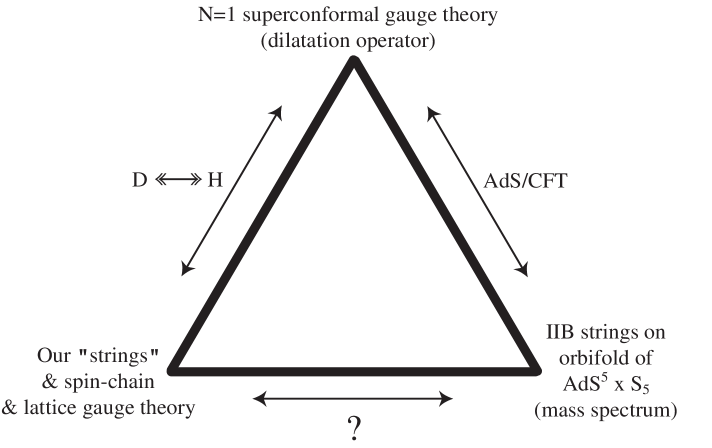
Figure 14: The dualities.

Appendix A Conventions

We present in this appendix our conventions and notation. $SU(N)$ traces satisfy

$$tr(T^{a}T^{b})=C(r)\delta^{ab}$$ (A.1)

with $C(r)$ the Dynkin index of the representation for the fields, equal to $N$ for the adjoint representation. Writing the adjoint fields of $U(N)$ as products of fundamental and anti-fundamentals allows us to write free propagators with the index structure (dropping the obvious space-time dependance):

$$\Big{<}\phi^{i}_{j}\phi^{k}_{l}\Big{>}_{0}\propto\delta^{i}_{l}\delta^{k}_{j}$$ (A.2)

for $U(N)$. For $SU(N)$ there is an extra term arising from the fact that all the generators are traceless. Subtracting the extra trace part gives

$$\Big{<}\phi^{i}_{j}\phi^{k}_{l}\Big{>}_{0}\propto\left(\delta^{i}_{l}\delta^{k}_{j}-\frac{1}{N}\delta^{i}_{j}\delta^{k}_{l}\right)$$ (A.3)

The extra term is subleading in the large $N$ limit, but in any case, because of the commutators in (3.3) we are free to use the $U(N)$ rules.

We also have the useful identity

$$tr\left(T^{a}[T^{b},T^{c}]\right)=iC(r)f^{abc}$$ (A.4)

where $f^{abc}$ are the structure constants. Note also that

$$\epsilon_{ijk}\epsilon_{ilm}=\delta^{jl}\delta^{km}-\delta^{jm}\delta^{kl}$$ (A.5)

summed over $i=1,2,3$.

Following these conventions, the $\mathcal{N}=4$ Lagrangian can be written in $\mathcal{N}=1$ language as follows:

$$S\>=\>\frac{1}{C(r)}\>tr \Bigg{[}\int d^{4}\theta\>\>e^{-g_{YM}V}\>\bar{\Phi}_{i}\>e^{g_{YM}V}\>\Phi_{i}$$ (A.6)

$$+\>\frac{1}{16g_{YM}^{2}}\left(\int d^{2}\theta\>\>W^{\alpha}W_{\alpha}\>+\>\int d^{2}\bar{\theta}\>\>\bar{W}_{\dot{\alpha}}\bar{W}^{\dot{\alpha}}\right)$$

$$+\>i\>g_{YM}\frac{\sqrt{2}}{3!}\epsilon_{ijk}\left(\int d^{2}\theta\>\>\Phi_{i}[\Phi_{j},\Phi_{k}]\>+\>\int d^{2}\bar{\theta}\>\>\bar{\Phi}_{i}[\bar{\Phi}_{j},\bar{\Phi}_{k}]\right)\Bigg{]}$$

The $\Phi_{i}$ are three chiral superfields and $V$ is a vector superfield, all transforming in the adjoint representation of $U(Npq)$.. The correct dependence on the coupling for the gauge kinetic terms is established after taking $V\rightarrow 2g_{YM}V$ in the second term.

When writing the $\mathcal{N}=4$ action in $\mathcal{N}=1$ language, the F-terms and D-terms are

$$\mathcal{L}_{D}\>=\>\frac{-1}{2g_{YM}^{2}}{{Tr}}\left([A,\bar{A}]\>+\>[B,\bar{B}]\>+\>[C,\bar{C}]\right)^{2}$$ (A.7)

with bars denoting conjugation, and

$$\mathcal{L}_{F}\>=\>\frac{1}{g_{YM}^{2}}{{Tr}}\left(|[A,B]|^{2}\>+\>|[A,C]|^{2}\>+\>\|[B,C]|^{2}\right)$$ (A.8)

The trace here is taken over $p\times q\times N$ by $p\times q\times N$ matrices. The F-terms arise from a superpotential of the form $Tr(ABC)$. As in the parent $\mathcal{N}=4$ theory, the gauge field loops, scalar self energies and D-term contributions cancel against each other. This is responsible for making the straight line operators BPS, as discussed in section 3.2.

The orbifolding in the gauge theory acts as a projection on these matrices. The square of the commutator terms in the F-terms appear as

$$|[A,B]|^{2}\>=\>[\bar{B}\>,\>\bar{A}][A\>,\>B]$$ (A.9)

A useful shorthand notation for capturing field contractions is to introduce variations with respect to the fields as follows

$$\delta_{m}=\frac{\delta}{\delta\phi_{m}}$$ (A.10)

The six real scalar fields $\phi_{m}$ are matrix valued $\phi_{m}=\phi_{m}^{a}T^{a}$, with $T^{a}$ being the generators of $U(Npq)$. This definition is motivated by analogy to Wick contractions in the form of free field propagators.

We find it convenient to work in terms of the complex scalars appearing in the three chiral superfields, letting

$$\Phi_{I}=\frac{1}{\sqrt{2}}\left(\phi_{2I-1}+i\phi_{2I}\right)\\$$ (A.11)

with $I=1,2,3$ and $\{\Phi_{I}\}=A,B,C$. Then the variations with respect to these complex fields are defined as

$$\Delta_{I}=\frac{1}{\sqrt{2}}\left(\frac{\delta}{\delta\phi_{2I-1}}-i\frac{\delta}{\delta\phi_{2I}}\right)$$ (A.12)

and the derivatives with respect to the conjugate fields are

$$\bar{\Delta}_{I}=\frac{1}{\sqrt{2}}\left(\frac{\delta}{\delta\phi_{2I-1}}+i\frac{\delta}{\delta\phi_{2I}}\right)$$ (A.13)

Since the Wick contractions of the scalars in non-zero only when we contract a field and its conjugate, we require that the variation $\Delta_{I}$ transform in the same way as $\bar{\Phi}_{I}$, i.e.​ in the conjugate representation, and therefore define $\Delta_{I}=\Delta_{I}^{a}\bar{T}^{a}$. Note that (as explained in section 3.1) the generators $T^{a}$ on the covering space are not hermitian. Note also that derivatives act as annihilation operators, and the fields and derivatives satisfy a creation-annihilation algebra. The example in Appendix B clarifies these points.

Appendix B Orbifolding Example

We give an explicit example of the orbifolding in the gauge theory, where we take $p=q=3$, for which there are $9$ lattice sites. The generators of the symmetry for the theory living on the covering space is the direct product of the generators of the original $U(9N)$ symmetry with the generators of $\mathbb{Z}_{3}\times\mathbb{Z}_{3}$ in the regular representation, leading to the generators

$$T^{A\alpha}\>=\>\left(\begin{matrix}0\>\>&\>\>T^{\alpha}_{1,1}\>\>&\>\>0\>\>&\>\>0\>\>&\>\>0\>\>&\>\>0\>\>&\>\>0\>\>&\>\>0\>\>&\>\>0\\ 0\>\>&\>\>0\>\>&\>\>T^{\alpha}_{1,2}\>\>&\>\>0\>\>&\>\>0\>\>&\>\>0\>\>&\>\>0\>\>&\>\>0\>\>&\>\>0\\ T^{\alpha}_{1,3}\>\>&\>\>0\>\>&\>\>0\>\>&\>\>0\>\>&\>\>0\>\>&\>\>0\>\>&\>\>0\>\>&\>\>0\>\>&\>\>0\\ 0\>\>&\>\>0\>\>&\>\>0\>\>&\>\>0\>\>&\>\>T^{\alpha}_{2,1}\>\>&\>\>0\>\>&\>\>0\>\>&\>\>0\>\>&\>\>0\\ 0\>\>&\>\>0\>\>&\>\>0\>\>&\>\>0\>\>&\>\>0\>\>&\>\>T^{\alpha}_{2,2}\>\>&\>\>0\>\>&\>\>0\>\>&\>\>0\\ 0\>\>&\>\>0\>\>&\>\>0\>\>&\>\>T^{\alpha}_{2,3}\>\>&\>\>0\>\>&\>\>0\>\>&\>\>0\>\>&\>\>0\>\>&\>\>0\\ 0\>\>&\>\>0\>\>&\>\>0\>\>&\>\>0\>\>&\>\>0\>\>&\>\>0\>\>&\>\>0\>\>&\>\>T^{\alpha}_{3,1}\>\>&\>\>0\\ 0\>\>&\>\>0\>\>&\>\>0\>\>&\>\>0\>\>&\>\>0\>\>&\>\>0\>\>&\>\>0\>\>&\>\>0\>\>&\>\>T^{\alpha}_{3,2}\\ 0\>\>&\>\>0\>\>&\>\>0\>\>&\>\>0\>\>&\>\>0\>\>&\>\>0\>\>&\>\>T^{\alpha}_{3,3}\>\>&\>\>0\>\>&\>\>0\end{matrix}\right)$$ (B.1)

$$T^{B\alpha}\>=\>\left(\begin{matrix}0\>\>&\>\>0\>\>&\>\>0\>\>&\>\>0\>\>&\>\>0\>\>&\>\>0\>\>&\>\>0\>\>&\>\>0\>\>&\>\>T^{\alpha}_{1,1}\\ 0\>\>&\>\>0\>\>&\>\>0\>\>&\>\>0\>\>&\>\>0\>\>&\>\>0\>\>&\>\>T^{\alpha}_{1,2}\>\>&\>\>0\>\>&\>\>0\\ 0\>\>&\>\>0\>\>&\>\>0\>\>&\>\>0\>\>&\>\>0\>\>&\>\>0\>\>&\>\>0\>\>&\>\>T^{\alpha}_{1,3}\>\>&\>\>0\\ 0\>\>&\>\>0\>\>&\>\>T^{\alpha}_{2,1}\>\>&\>\>0\>\>&\>\>0\>\>&\>\>0\>\>&\>\>0\>\>&\>\>0\>\>&\>\>0\\ T^{\alpha}_{2,2}\>\>&\>\>0\>\>&\>\>0\>\>&\>\>0\>\>&\>\>0\>\>&\>\>0\>\>&\>\>0\>\>&\>\>0\>\>&\>\>0\\ 0\>\>&\>\>T^{\alpha}_{2,3}\>\>&\>\>0\>\>&\>\>0\>\>&\>\>0\>\>&\>\>0\>\>&\>\>0\>\>&\>\>0\>\>&\>\>0\\ 0\>\>&\>\>0\>\>&\>\>0\>\>&\>\>0\>\>&\>\>0\>\>&\>\>T^{\alpha}_{3,1}\>\>&\>\>0\>\>&\>\>0\>\>&\>\>0\\ 0\>\>&\>\>0\>\>&\>\>0\>\>&\>\>T^{\alpha}_{3,2}\>\>&\>\>0\>\>&\>\>0\>\>&\>\>0\>\>&\>\>0\>\>&\>\>0\\ 0\>\>&\>\>0\>\>&\>\>0\>\>&\>\>0\>\>&\>\>T^{\alpha}_{3,3}\>\>&\>\>0\>\>&\>\>0\>\>&\>\>0\>\>&\>\>0\end{matrix}\right)$$ (B.2)

$$T^{C\alpha}\>=\>\left(\begin{matrix}0\>\>&\>\>0\>\>&\>\>0\>\>&\>\>T^{\alpha}_{1,1}\>\>&\>\>0\>\>&\>\>0\>\>&\>\>0\>\>&\>\>0\>\>&\>\>0\\ 0\>\>&\>\>0\>\>&\>\>0\>\>&\>\>0\>\>&\>\>T^{\alpha}_{1,2}\>\>&\>\>0\>\>&\>\>0\>\>&\>\>0\>\>&\>\>0\\ 0\>\>&\>\>0\>\>&\>\>0\>\>&\>\>0\>\>&\>\>0\>\>&\>\>T^{\alpha}_{1,3}\>\>&\>\>0\>\>&\>\>0\>\>&\>\>0\\ 0\>\>&\>\>0\>\>&\>\>0\>\>&\>\>0\>\>&\>\>0\>\>&\>\>0\>\>&\>\>T^{\alpha}_{2,1}\>\>&\>\>0\>\>&\>\>0\\ 0\>\>&\>\>0\>\>&\>\>0\>\>&\>\>0\>\>&\>\>0\>\>&\>\>0\>\>&\>\>0\>\>&\>\>T^{\alpha}_{2,2}\>\>&\>\>0\\ 0\>\>&\>\>0\>\>&\>\>0\>\>&\>\>0\>\>&\>\>0\>\>&\>\>0\>\>&\>\>0\>\>&\>\>0\>\>&\>\>T^{\alpha}_{2,3}\\ T^{\alpha}_{3,1}\>\>&\>\>0\>\>&\>\>0\>\>&\>\>0\>\>&\>\>0\>\>&\>\>0\>\>&\>\>0\>\>&\>\>0\>\>&\>\>0\\ 0\>\>&\>\>T^{\alpha}_{3,2}\>\>&\>\>0\>\>&\>\>0\>\>&\>\>0\>\>&\>\>0\>\>&\>\>0\>\>&\>\>0\>\>&\>\>0\\ 0\>\>&\>\>0\>\>&\>\>T^{\alpha}_{3,3}\>\>&\>\>0\>\>&\>\>0\>\>&\>\>0\>\>&\>\>0\>\>&\>\>0\>\>&\>\>0\end{matrix}\right)$$ (B.3)

The conjugate representation is generated by

$$\bar{T}^{A\alpha}\>=\>\left(\begin{matrix}0\>\>&\>\>0\>\>&\>\>\bar{T}^{\alpha}_{1,3}\>\>&\>\>0\>\>&\>\>0\>\>&\>\>0\>\>&\>\>0\>\>&\>\>0\>\>&\>\>0\\ \bar{T}^{\alpha}_{1,1}\>\>&\>\>0\>\>&\>\>0\>\>&\>\>0\>\>&\>\>0\>\>&\>\>0\>\>&\>\>0\>\>&\>\>0\>\>&\>\>0\\ 0\>\>&\>\>\bar{T}^{\alpha}_{1,2}\>\>&\>\>0\>\>&\>\>0\>\>&\>\>0\>\>&\>\>0\>\>&\>\>0\>\>&\>\>0\>\>&\>\>0\\ 0\>\>&\>\>0\>\>&\>\>0\>\>&\>\>0\>\>&\>\>0\>\>&\>\>\bar{T}^{\alpha}_{2,3}\>\>&\>\>0\>\>&\>\>0\>\>&\>\>0\\ 0\>\>&\>\>0\>\>&\>\>0\>\>&\>\>\bar{T}^{\alpha}_{2,1}\>\>&\>\>0\>\>&\>\>0\>\>&\>\>0\>\>&\>\>0\>\>&\>\>0\\ 0\>\>&\>\>0\>\>&\>\>0\>\>&\>\>0\>\>&\>\>\bar{T}^{\alpha}_{2,2}\>\>&\>\>0\>\>&\>\>0\>\>&\>\>0\>\>&\>\>0\\ 0\>\>&\>\>0\>\>&\>\>0\>\>&\>\>0\>\>&\>\>0\>\>&\>\>0\>\>&\>\>0\>\>&\>\>0\>\>&\>\>\bar{T}^{\alpha}_{3,3}\\ 0\>\>&\>\>0\>\>&\>\>0\>\>&\>\>0\>\>&\>\>0\>\>&\>\>0\>\>&\>\>\bar{T}^{\alpha}_{3,1}\>\>&\>\>0\>\>&\>\>0\\ 0\>\>&\>\>0\>\>&\>\>0\>\>&\>\>0\>\>&\>\>0\>\>&\>\>0\>\>&\>\>0\>\>&\>\>\bar{T}^{\alpha}_{3,2}\>\>&\>\>0\end{matrix}\right)$$ (B.4)

$$\bar{T}^{B\alpha}\>=\>\left(\begin{matrix}0\>\>&\>\>0\>\>&\>\>0\>\>&\>\>0\>\>&\>\>\bar{T}^{\alpha}_{2,2}\>\>&\>\>0\>\>&\>\>0\>\>&\>\>0\>\>&\>\>0\\ 0\>\>&\>\>0\>\>&\>\>0\>\>&\>\>0\>\>&\>\>0\>\>&\>\>\bar{T}^{\alpha}_{2,3}\>\>&\>\>0\>\>&\>\>0\>\>&\>\>0\\ 0\>\>&\>\>0\>\>&\>\>0\>\>&\>\>\bar{T}^{\alpha}_{2,1}\>\>&\>\>0\>\>&\>\>0\>\>&\>\>0\>\>&\>\>0\>\>&\>\>0\\ 0\>\>&\>\>0\>\>&\>\>0\>\>&\>\>0\>\>&\>\>0\>\>&\>\>0\>\>&\>\>0\>\>&\>\>\bar{T}^{\alpha}_{3,2}\>\>&\>\>0\\ 0\>\>&\>\>0\>\>&\>\>0\>\>&\>\>0\>\>&\>\>0\>\>&\>\>0\>\>&\>\>0\>\>&\>\>0\>\>&\>\>\bar{T}^{\alpha}_{3,3}\\ 0\>\>&\>\>0\>\>&\>\>0\>\>&\>\>0\>\>&\>\>0\>\>&\>\>0\>\>&\>\>\bar{T}^{\alpha}_{3,1}\>\>&\>\>0\>\>&\>\>0\\ 0\>\>&\>\>\bar{T}^{\alpha}_{1,2}\>\>&\>\>0\>\>&\>\>0\>\>&\>\>0\>\>&\>\>0\>\>&\>\>0\>\>&\>\>0\>\>&\>\>0\\ 0\>\>&\>\>0\>\>&\>\>\bar{T}^{\alpha}_{1,3}\>\>&\>\>0\>\>&\>\>0\>\>&\>\>0\>\>&\>\>0\>\>&\>\>0\>\>&\>\>0\\ \bar{T}^{\alpha}_{1,1}\>\>&\>\>0\>\>&\>\>0\>\>&\>\>0\>\>&\>\>0\>\>&\>\>0\>\>&\>\>0\>\>&\>\>0\>\>&\>\>0\end{matrix}\right)$$ (B.5)

$$\bar{T}^{C\alpha}\>=\>\left(\begin{matrix}0\>\>&\>\>0\>\>&\>\>0\>\>&\>\>0\>\>&\>\>0\>\>&\>\>0\>\>&\>\>\bar{T}^{\alpha}_{3,1}\>\>&\>\>0\>\>&\>\>0\\ 0\>\>&\>\>0\>\>&\>\>0\>\>&\>\>0\>\>&\>\>0\>\>&\>\>0\>\>&\>\>0\>\>&\>\>\bar{T}^{\alpha}_{3,2}\>\>&\>\>0\\ 0\>\>&\>\>0\>\>&\>\>0\>\>&\>\>0\>\>&\>\>0\>\>&\>\>0\>\>&\>\>0\>\>&\>\>0\>\>&\>\>\bar{T}^{\alpha}_{3,3}\\ \bar{T}^{\alpha}_{1,1}\>\>&\>\>0\>\>&\>\>0\>\>&\>\>0\>\>&\>\>0\>\>&\>\>0\>\>&\>\>0\>\>&\>\>0\>\>&\>\>0\\ 0\>\>&\>\>\bar{T}^{\alpha}_{1,2}\>\>&\>\>0\>\>&\>\>0\>\>&\>\>0\>\>&\>\>0\>\>&\>\>0\>\>&\>\>0\>\>&\>\>0\\ 0\>\>&\>\>0\>\>&\>\>\bar{T}^{\alpha}_{1,3}\>\>&\>\>0\>\>&\>\>0\>\>&\>\>0\>\>&\>\>0\>\>&\>\>0\>\>&\>\>0\\ 0\>\>&\>\>0\>\>&\>\>0\>\>&\>\>\bar{T}^{\alpha}_{2,1}\>\>&\>\>0\>\>&\>\>0\>\>&\>\>0\>\>&\>\>0\>\>&\>\>0\\ 0\>\>&\>\>0\>\>&\>\>0\>\>&\>\>0\>\>&\>\>\bar{T}^{\alpha}_{2,2}\>\>&\>\>0\>\>&\>\>0\>\>&\>\>0\>\>&\>\>0\\ 0\>\>&\>\>0\>\>&\>\>0\>\>&\>\>0\>\>&\>\>0\>\>&\>\>\bar{T}^{\alpha}_{2,3}\>\>&\>\>0\>\>&\>\>0\>\>&\>\>0\end{matrix}\right)$$ (B.6)

The index $\alpha$ runs over the generators of $U(N)$. In the notation used above all the $T^{\alpha}_{i,j}$ for any $i,j$ are in fact the same when considered as generators of $U(N)$, but the notation is meant as a reminder that they act only as generators of the $U(N)$ group at the lattice site denoted by $i,j$.

Diagonal elements correspond to adjoint fields and the off-diagonal elements to bi-fundamentals. The row and column indices of the matrix can be derived by flattening the $i,j$ coordinates via $i,j\rightarrow\left[\left(i-1\right)\times q\right]+j$. In this notation we identify $i=0$ with $i=p$ and $j=0$ with $j=q$. When writing things in matrix form, the fundamental index indicates the row and the anti-fundamental index the column, for both fields and their conjugates. When multiplying matrices, it is important to note that

$$\left(N_{i,j}\>,\>\bar{N}_{k,l}\right)\otimes\left(N_{k,l}\>,\>\bar{N}_{m,n}\right)\>\sim\>\left(N_{i,j}\>,\>\bar{N}_{m,n}\right)\ .$$ (B.7)

Making use of these generators, we can now explicitly construct the one-loop correction to the dilatation operator. Starting with (3.5) and evaluating the trace after the orbifolding gives rise to a sum of terms, each situated at a lattice site, and a trace over $N\times N$ matrices associated to the gauge group sitting at the sites. This is a $3\times 3$ triangular lattice, of the form discussed in section 2.1. In general, there are many terms which appear in this sum. These terms are more easily described in terms of “interaction” plaquettes on the lattice, as described in section 3.2. We are primarily interested in terms which give non-vanishing contributions when acting on purely holomorphic operators. These arise from the first term in (3.5), with the second term giving similar non-vanishing terms when acting on purely anti-holomorphic operators. The other terms in $\mathfrak{D}_{1}$ have one holomorphic and one anti-holomorphic derivative, and so vanish when acting on operators with only holomorphic or only anti-holomorphic fields. We summarize the terms of interest for holomorphic operators

$$\mathfrak{D}_{1}=2\>\sum_{i,j}tr\Big{(} B_{i+1,j+1}A_{i,j}\Delta^{A}_{i,j}\Delta^{B}_{i+1,j+1}$$ (B.8)

$$\>- A_{ij}B_{i,j+1}\Delta^{A}_{i-1,j-1}\Delta^{B}_{i,j}$$

$$\>- B_{i+1,j+1}A_{i,j}\Delta^{B}_{i+1,j+2}\Delta^{A}_{i+1,j+1}$$

$$\>+ A_{i,j}B_{i,j+1}\Delta^{B}_{i,j+1}\Delta^{A}_{i,j}$$

$$\>+ C_{i-1,j}A_{i,j}\Delta^{A}_{i,j}\Delta^{C}_{i-1,j}$$

$$\>- A_{i,j}C_{i,j+1}\Delta^{A}_{i+1,j}\Delta^{C}_{i,j}$$

$$\>- C_{i-1,j}A_{i,j}\Delta^{C}_{i-1,j+1}\Delta^{A}_{i-1,j}$$

$$\>+ A_{i,j}C_{i,j+1}\Delta^{C}_{i,j+1}\Delta^{A}_{i,j}$$

$$\>+ C_{i-1,j}B_{i,j}\Delta^{B}_{i,j}\Delta^{C}_{i-1,j}$$

$$\>- B_{i,j}C_{i-1,j-1}\Delta^{B}_{i+1,j}\Delta^{C}_{i,j}$$

$$\>- C_{i-1,j}B_{i,j}\Delta^{C}_{i-2,j-1}\Delta^{B}_{i-1,j}$$

$$\>+ B_{i,j}C_{i-1,j-1}\Delta^{C}_{i-1,j-1}\Delta^{B}_{i,j}\Big{)}\ .$$

The sum above is over all lattice sites, and we impose periodic boundary conditions as before. Each field appearing above takes values in the lie algebra of $U(N)$, and $tr$ denotes a trace over the $U(N)$ indices. For example, $A_{i,j}$ is an $U(N)$ lie algebra element sitting on the $A_{i,j}$ link, and under a gauge transformation the field $A_{i,j}$ transforms as $A_{i,j}\rightarrow U_{i,j}A_{i,j}U^{\dagger}_{i,j+1}$, with the subscripts on the $U$’s denoting the gauge group whose transformations they generate, as appropriate for bi-fundamental fields. Similar rules apply to the other fields (see (2.1) for their transformation properties). Using these rules it is easy to see that each term in (B.8) is gauge invariant.

Examples of terms which only give non-zero contributions when acting on operators with both holomorphic and anti-holomorphic fields are $tr(A_{i,j}\bar{\Delta}^{B}_{i,j+1}\bar{A}_{i-1,j-1}\Delta^{B}_{i,j})$ and $tr(A_{i,j}\Delta^{B}_{i+1,j+2}\bar{A}_{i+1,j+1}\bar{\Delta}^{B}_{i+1,j+1})$. Note that for such operators it is not necessary for the solid (likewise dashed) lines to touch each other. They generally lead to $1/N$ non-planar interactions. Other examples are $tr(A_{i,j}\bar{B}_{i+1,j+2}\Delta^{A}_{i+1,j+1}\bar{\Delta}^{B}_{i+1,j+1})$ which has a similar structure to the open plaquettes already discussed, aside from the appearance of mixed fields, and new “flat” plaquettes of the form $tr(A_{i,j}\bar{A}_{i,j}\Delta^{A}_{i,j-1}\bar{\Delta}^{A}_{i,j-1})$ and $tr(A_{i,j}\bar{A}_{i,j}\bar{\Delta}^{A}_{i,j}\Delta^{A}_{i,j})$. These terms are depicted in Figure 7.

We now give two examples that demonstrates how an interaction plaquette acts on composite operators. For this we need to know how the Wick contractions act. Following the definitions in the previous appendix, we have

$$\left(\Delta^{I}_{kl}\right)^{ab}\left(\Phi^{J}_{mn}\right)^{cd}\>=\>\delta^{IJ}\ \delta_{km}\ \delta_{ln}\ \delta^{ad}\ \delta^{bc}$$ (B.9)

with $I,J$ ranging over $A,B,C$, $(k,l),(m,n)$ the lattice coordinates, and $(a,b),(c,d)$ $N\times N$ matrix indices. Consider now an operator of the form

$$O=tr:\left(\bar{C}_{1,1}\bar{B}_{2,2}C_{2,2}B_{3,2}\right):\ ,$$ (B.10)

together with the interaction term

$$I=tr:\left(\Delta^{B}_{3,2}\Delta^{C}_{2,2}B_{2,2}C_{1,1}\right):\ ,$$ (B.11)

which is one possible interaction term of the form appearing in figure 3. The interaction term $I$ operates on $O$ as follows

$$I\ O=N\>tr:\left(B_{2,2}C_{1,1}\bar{C}_{1,1}\bar{B}_{2,2}\right):\ .$$ (B.12)

The factor of $N$ shows that this contraction is at planar level. Here the single factor of $N$ arises from the contraction of two derivatives in a single trace from the interaction with two fields in another single trace.

A planar example involving one of the plaquettes in Figure 7 is given by

$$I=tr:\left(A_{1,2}\bar{A}_{1,2}\Delta^{A}_{1,1}\bar{\Delta}^{A}_{1},1\right):$$ (B.13)

and

$$O=tr:\left(A_{1,1}A_{1,2}\bar{A}_{1,2}\bar{A}_{1,1}\right):$$ (B.14)

Then

$$I\ O=N\>tr:\left(A_{1,2}\bar{A}_{1,2}A_{1,2}\bar{A}_{1,2}\right):$$ (B.15)

For a final example that involves non-holomorphic operators as well as non-planar interactions consider

$$O=tr:\left(A_{2,2}B_{2,3}\bar{A}_{1,1}\bar{C}_{2,2}\right):tr:\left(\bar{A}_{2,1}\bar{C}_{3,2}A_{3,2}B_{3,3}\right):\ ,$$ (B.16)

which is a double trace operator representing two closed strings on the lattice. Take the interaction term to be

$$I=tr:\left(A_{2,2}\Delta^{A}_{2,2}\Delta^{B}_{3,3}B_{3,3}\right):\ .$$ (B.17)

Using the above rules for contractions, we arrive at

$$I\ O=tr:\left(A_{2,2}B_{2,3}\bar{A}_{1,1}C_{2,2}\bar{A}_{2,1}\bar{C}_{3,2}A_{3,2}B_{3,3}\right):\ .$$ (B.18)

This operator is suppressed by one power of $N$ relative to the previous one, showing that it is non-planar, and involves the joining of two strings into one. Here the non-planar dependence on $N$ is due to the fact that the two derivatives inside the single trace interaction operator acts on two fields in different traces, and it costs one factor of $1/N$ to join these traces. This how strings join and split.

Finally, we would like to comment on the general case of an asymmetric orbifold, where $p\neq q$. In this case the boundary conditions break the $\mathbb{Z}_{3}$ rotational symmetry of the lattice theory. The dilatation operator when expanded on the lattice then also contains terms which are no longer invariant under the $\mathbb{Z}_{3}$ symmetry relabeling the fields.

References

- [1] J. M. Maldacena, “The large N limit of superconformal field theories and supergravity,” Adv. Theor. Math. Phys. 2, 231 (1998) [Int. J. Theor. Phys. 38, 1113 (1999)] [arXiv:hep-th/9711200]. S. S. Gubser, I. R. Klebanov and A. M. Polyakov, “Gauge theory correlators from non-critical string theory,” Phys. Lett. B 428, 105 (1998) [arXiv:hep-th/9802109]. E. Witten, “Anti-de Sitter space and holography,” Adv. Theor. Math. Phys. 2, 253 (1998) [arXiv:hep-th/9802150].
- [2] O. Aharony, S. S. Gubser, J. M. Maldacena, H. Ooguri and Y. Oz, “Large N field theories, string theory and gravity,” Phys. Rept. 323, 183 (2000) [arXiv:hep-th/9905111].
- [3] D. Berenstein, J. M. Maldacena and H. Nastase, “Strings in flat space and pp waves from N = 4 super Yang Mills,” JHEP 0204, 013 (2002) [arXiv:hep-th/0202021].
- [4] J. C. Plefka, “Lectures on the plane-wave string / gauge theory duality,” Fortsch. Phys. 52, 264 (2004) [arXiv:hep-th/0307101].
- [5] D. Sadri and M. M. Sheikh-Jabbari, “The plane-wave / super Yang-Mills duality,” Rev. Mod. Phys. 76, 853 (2004) [arXiv:hep-th/0310119].
- [6] N. Beisert, C. Kristjansen and M. Staudacher, “The dilatation operator of N = 4 super Yang-Mills theory,” Nucl. Phys. B 664, 131 (2003) [arXiv:hep-th/0303060].
- [7] N. Beisert, “The complete one-loop dilatation operator of N = 4 super Yang-Mills theory,” Nucl. Phys. B 676, 3 (2004) [arXiv:hep-th/0307015].
- [8] J. A. Minahan and K. Zarembo, “The Bethe-ansatz for N = 4 super Yang-Mills,” JHEP 0303, 013 (2003) [arXiv:hep-th/0212208].
- [9] N. Beisert, “The dilatation operator of N = 4 super Yang-Mills theory and integrability,” Phys. Rept. 405, 1 (2005) [arXiv:hep-th/0407277].
- [10] N. Beisert and M. Staudacher, “The N = 4 SYM integrable super spin chain,” Nucl. Phys. B 670, 439 (2003) [arXiv:hep-th/0307042].
- [11] S. Frolov and A. A. Tseytlin, “Multi-spin string solutions in AdS(5) x S**5,” Nucl. Phys. B 668 (2003) 77 [arXiv:hep-th/0304255]. G. Arutyunov, S. Frolov, J. Russo and A. A. Tseytlin, “Spinning strings in AdS(5) x S**5 and integrable systems,” Nucl. Phys. B 671 (2003) 3 [arXiv:hep-th/0307191]. M. Kruczenski, “Spin chains and string theory,” Phys. Rev. Lett. 93, 161602 (2004) [arXiv:hep-th/0311203].
- [12] M. Kruczenski, “Spiky strings and single trace operators in gauge theories,” arXiv:hep-th/0410226.
- [13] I. Bena, J. Polchinski and R. Roiban, “Hidden symmetries of the AdS(5) x S**5 superstring,” Phys. Rev. D 69, 046002 (2004) [arXiv:hep-th/0305116].
- [14] N. Beisert, “Higher loops, integrability and the near BMN limit,” JHEP 0309, 062 (2003) [arXiv:hep-th/0308074]; N. Beisert, “The su(23) dynamic spin chain,” Nucl. Phys. B 682, 487 (2004) [arXiv:hep-th/0310252].
- [15] N. Beisert, V. Dippel and M. Staudacher, “A novel long range spin chain and planar N = 4 super Yang-Mills,” JHEP 0407, 075 (2004) [arXiv:hep-th/0405001]. N. Beisert and M. Staudacher, “Long-range PSU(2,24) Bethe ansaetze for gauge theory and strings,” arXiv:hep-th/0504190.
- [16] H. Bethe, Z. Phys. 71, 205 (1931).
- [17] J. A. Minahan, “Higher loops beyond the SU(2) sector,” JHEP 0410, 053 (2004) [arXiv:hep-th/0405243]. C. G. . Callan, T. McLoughlin and I. Swanson, “Higher impurity AdS/CFT correspondence in the near-BMN limit,” Nucl. Phys. B 700, 271 (2004) [arXiv:hep-th/0405153]. T. McLoughlin and I. Swanson, “N-impurity superstring spectra near the pp-wave limit,” Nucl. Phys. B 702, 86 (2004) [arXiv:hep-th/0407240].
- [18] G. Arutyunov, S. Frolov and M. Staudacher, “Bethe ansatz for quantum strings,” JHEP 0410 (2004) 016 [arXiv:hep-th/0406256]. N. Beisert and A. A. Tseytlin, “On quantum corrections to spinning strings and Bethe equations,” arXiv:hep-th/0509084. J. A. Minahan, A. Tirziu and A. A. Tseytlin, “1/J corrections to semiclassical AdS/CFT states from quantum Landau-Lifshitz model,” arXiv:hep-th/0509071; “1/J**2 corrections to BMN energies from the quantum long range Landau-Lifshitz model,” arXiv:hep-th/0510080. S. Schafer-Nameki, M. Zamaklar and K. Zarembo, “Quantum corrections to spinning strings in and Bethe ansatz: A comparative study,” JHEP 0509 (2005) 051 [arXiv:hep-th/0507189]. S. Schafer-Nameki and M. Zamaklar, “Stringy sums and corrections to the quantum string Bethe ansatz,” arXiv:hep-th/0509096.
-
[19]
L. Dolan, A New Symmetry Group of Real Self-dual Yang-Mills,
Phys. Lett. 113B (1982) 273.
L.L. Chau, M.L. Ge and Y.S. Wu, Kac-Moody Algebra in the Self-dual Yang-Mills Equation, Phys. Rev. D25 (1982) 1086;
L.L. Chau and Y.S. Wu, More about Hidden Symmetry Algebra for the Self-Dual Yang-Mills System Phys. Rev. D26 (1982) 3581;
L.L. Chau, M.L. Ge, A. Sinha and Y.S. Wu, Hidden Symmetry Algebra for Self-Dual Yang-Mills Equations Phys. Lett. 121B (1983) 391.
H.C. Tze and Y.S. Wu, Infinite Number of Local Conservation Laws for the Self-dual Yang-Mills Systems, Nucl. Phys. B204 (1982) 118.
K. Ueno and Y. Nakamura, Transformation Theory for (Anti)Self-dual Equations and the Riemann-Hilbert Problem, Phys. Lett. 109B (1982) 273.
J. Avan, H.J. de Vega and J.M. Maillet. Conformally Covariant Linear System for the Four-Dimensional Self-Dual Yang-Mills Theory, Phys. Lett. 171B (1986) 255.
W.A. Bardeen, Selfdual Yang-Mills Theory, Integrability and Multiparton Ampilitudes, Prog. Theor. Phys. Suppl. bf 123 (1996) 1.
A.D. Popov and C.R. Preitschopf, Conformal Symmetries of the Self-Dual Yang-Mills Equations, Phys. Lett. B374 (1996) 71; A.D. Popov, Self-Dual Yang-Mills: Symmetries and Moduli Space, Rev. Math. Phys. 11 (1999) 1091. -
[20]
L.N. Lipatov, High-energy Asymptotics of Multicolor QCD and
Exactly Solvable Lattice Models, JETP Lett. 59 (1994)
596.
L.D. Faddev and G.P. Korchemsky, High-energy QCD as a Completely Integrable Model, Phys. Lett. B342 (1995) 311.
A.V. Belitsky, A.S. Gorsky and G.P. Korchemsky, Gauge / String Duality For QCD Conformal Operators, Nucl. Phys. B667 (2003) 3.
V.M. Braun, S.E. Derkachov and A.N. Manashov, Integrability Of Three Particle Evolution Equations In QCD, Phys. Rev. Lett. 81 (1998) 2020; V.M. Braun, S.E. Derkachov, G.P. Korchemsky and A.N. Manashov, Baryon Distribution Amplitudes In QCD, Nucl. Phys. B553 (1999) 355; A.V. Belitsky, Renormalization Of Twist - Three Operators And Integrable Lattice Models, Nucl. Phys. B574 (2000) 407; S.E. Derkachov, G.P. Korchemsky and A.N. Manashov, Evolution Equations For Quark Gluon Distributions In Multicolor QCD And Open Spin Chain, Nucl. Phys. B566 (2000) 203. - [21] N. Beisert, G. Ferretti, R. Heise and K. Zarembo, “One-loop QCD spin chain and its spectrum,” Nucl. Phys. B 717, 137 (2005) [arXiv:hep-th/0412029].
- [22] A.V. Kotikov, L.N. Lipatov and V.N. Velizhanin, Anomalous Dimensions of Wilson Operators in SYM theory, Phys. Lett. B557 (2003) 114.
- [23] M. R. Douglas and G. W. Moore, “D-branes, Quivers, and ALE Instantons,” arXiv:hep-th/9603167.
- [24] S. Kachru and E. Silverstein, “4d conformal theories and strings on orbifolds,” Phys. Rev. Lett. 80, 4855 (1998) [arXiv:hep-th/9802183].
- [25] A. E. Lawrence, N. Nekrasov and C. Vafa, “On conformal field theories in four dimensions,” Nucl. Phys. B 533, 199 (1998) [arXiv:hep-th/9803015]. Z. Kakushadze, “Gauge theories from orientifolds and large N limit,” Nucl. Phys. B 529, 157 (1998) [arXiv:hep-th/9803214]. M. Bershadsky and A. Johansen, “Large N limit of orbifold field theories,” Nucl. Phys. B 536, 141 (1998) [arXiv:hep-th/9803249].
- [26] S. Benvenuti and M. Kruczenski, “From Sasaki-Einstein spaces to quivers via BPS geodesics: L(p,qr),” arXiv:hep-th/0505206; “Semiclassical strings in Sasaki-Einstein manifolds and long operators in gauge theories,” arXiv:hep-th/0505046.
- [27] X. J. Wang and Y. S. Wu, “Integrable spin chain and operator mixing in N = 1,2 supersymmetric theories,” Nucl. Phys. B 683, 363 (2004) [arXiv:hep-th/0311073].
- [28] B. Chen, X. J. Wang and Y. S. Wu, “Integrable open spin chain in super Yang-Mills and the plane-wave / SYM duality,” JHEP 0402, 029 (2004) [arXiv:hep-th/0401016].
- [29] G. De Risi, G. Grignani, M. Orselli and G. W. Semenoff, “DLCQ string spectrum from N = 2 SYM theory,” arXiv:hep-th/0409315.
- [30] M. Bertolini, J. de Boer, T. Harmark, E. Imeroni and N. A. Obers, “Gauge theory description of compactified pp-waves,” JHEP 0301, 016 (2003) [arXiv:hep-th/0209201].
- [31] A. Hanany and A. Zaffaroni, “On the realization of chiral four-dimensional gauge theories using branes,” JHEP 9805, 001 (1998) [arXiv:hep-th/9801134].
- [32] N. Itzhaki, I. R. Klebanov and S. Mukhi, “PP wave limit and enhanced supersymmetry in gauge theories,” JHEP 0203, 048 (2002) [arXiv:hep-th/0202153]. M. Alishahiha and M. M. Sheikh-Jabbari, “The pp-wave limits of orbifolded AdS(5) x S(5),” Phys. Lett. B 535, 328 (2002) [arXiv:hep-th/0203018] N. w. Kim, A. Pankiewicz, S. J. Rey and S. Theisen, “Superstring on pp-wave orbifold from large-N quiver gauge theory,” Eur. Phys. J. C 25, 327 (2002) [arXiv:hep-th/0203080]. K. Oh and R. Tatar, “Orbifolds, Penrose limits and supersymmetry enhancement,” Phys. Rev. D 67, 026001 (2003) [arXiv:hep-th/0205067]. M. Alishahiha, M. M. Sheikh-Jabbari and R. Tatar, “Spacetime quotients, Penrose limits and conformal symmetry restoration,” JHEP 0301, 028 (2003) [arXiv:hep-th/0211285].
- [33] S. Mukhi, M. Rangamani and E. Verlinde, “Strings from quivers, membranes from moose,” JHEP 0205, 023 (2002) [arXiv:hep-th/0204147]. M. Alishahiha, M. M. Sheikh-Jabbari, “Strings in PP-waves and worldsheet deconstruction,” Phys. Lett. B 538, 180 (2002) [arXiv:hep-th/0204174].
- [34] J. B. Kogut, “An Introduction To Lattice Gauge Theory And Spin Systems,” Rev. Mod. Phys. 51, 659 (1979).
- [35] D. E. Diaconescu, M. R. Douglas and J. Gomis, “Fractional branes and wrapped branes,” JHEP 9802, 013 (1998) [arXiv:hep-th/9712230].
- [36] J. Wess and J. Bagger, “Supersymmetry and supergravity,” Princeton University Press; 2nd Rev. edition (March 3, 1992).
- [37] A. Hanany and E. Witten, “Type IIB superstrings, BPS monopoles, and three-dimensional gauge dynamics,” Nucl. Phys. B 492, 152 (1997) [arXiv:hep-th/9611230].
- [38] A. Hanany and A. M. Uranga, “Brane boxes and branes on singularities,” JHEP 9805, 013 (1998) [arXiv:hep-th/9805139].
- [39] P.R. Kulish and N.Yu. Reshetikin, Generalized Heisenberg Ferromagnet and the Gross-Neveu model, Sov. Phys. JETP 53 (1981) 108.
- [40] L.D. Faddeev, How Algebraic Bethe Ansatz Works for Integrable Model, hep-th/9605187.
- [41] O. Aharony, A. Hanany and B. Kol, “Webs of (p,q) 5-branes, five dimensional field theories and grid diagrams,” JHEP 9801, 002 (1998) [arXiv:hep-th/9710116].
- [42] J. Erlich, A. Hanany and A. Naqvi, “Marginal deformations from branes,” JHEP 9903, 008 (1999) [arXiv:hep-th/9902118].
- [43] B. Feng, A. Hanany and Y. H. He, “The Z(k) x D(k’) brane box model,” JHEP 9909, 011 (1999) [arXiv:hep-th/9906031].
- [44] B. Feng, A. Hanany and Y. H. He, “Z-D brane box models and non-chiral dihedral quivers,” arXiv:hep-th/9909125.
- [45] S. Hellerman, “Lattice gauge theories have gravitational duals,” arXiv:hep-th/0207226.
- [46] D. B. Kaplan, E. Katz and M. Unsal, “Supersymmetry on a spatial lattice,” JHEP 0305, 037 (2003) [arXiv:hep-lat/0206019]. D. B. Kaplan and M. Unsal, “A Euclidean lattice construction of supersymmetric Yang-Mills theories with sixteen supercharges,” JHEP 0509, 042 (2005) [arXiv:hep-lat/0503039]. M. Unsal, “Regularization of non-commutative SYM by orbifolds with discrete torsion and SL(2,Z) duality,” arXiv:hep-th/0409106.
- [47] N. Arkani-Hamed, A. G. Cohen, D. B. Kaplan, A. Karch and L. Motl,“Deconstructing (2,0) and little string theories,” JHEP 0301, 083 (2003) [arXiv:hep-th/0110146].
- [48] M. B. Halpern and W. Siegel, “Electromagnetism As A Strong Interaction,” Phys. Rev. D 11, 2967 (1975).
- [49] A. Hanany and K. D. Kennaway, “Dimer models and toric diagrams,” arXiv:hep-th/0503149. S. Franco, A. Hanany, K. D. Kennaway, D. Vegh and B. Wecht, “Brane dimers and quiver gauge theories,” arXiv:hep-th/0504110. S. Franco, A. Hanany, D. Martelli, J. Sparks, D. Vegh and B. Wecht, “Gauge theories from toric geometry and brane tilings,” arXiv:hep-th/0505211. T. Muto, “A relation between moduli space of D-branes on orbifolds and Ising model,” arXiv:hep-th/0508248.