On curvature coupling and quintessence fine-tuning

Abstract

We discuss the phenomenological model in which the potential energy of the quintessence field depends linearly on the energy density of the spatial curvature. We find that the pressure of the scalar field takes a different form when the potential of the scalar field also depends on the scale factor and the energy momentum tensor of the scalar field can be expressed as the form of a perfect fluid. A general coupling is proposed to explain the current accelerating expansion of the Universe and solve the fine-tuning problem.

The astronomical observations tell us that the Universe is currently expanding in an acceleration phase, while it was in a deceleration phase in the near past [1, 2]. The accelerating expansion of the Universe suggests that 70% of the total matter energy density comes from dark energy (DE) whose pressure is negative. The simplest candidate of DE is the cosmological constant. Due to the unusually small value of the cosmological constant given by observations, other DE models are explored, such as the quintessence models [3] and the holographic DE models [4, 5]. For a review of DE models, please see Ref. [6] and references therein.

The quintessence models employ a scalar field that slowly rolls down its potential well to explain the accelerating expansion. In the quintessence model, the potential energy dominates the energy component, so the current value of the potential energy must be of the order of the current critical energy density $3m_{p}^{2}H^{2}_{0}=8.1h^{2}\times 10^{-47}$ GeV⁴, where the reduced Planck mass $m_{p}=(8\pi G)^{-1/2}=1.221\times 10^{18}$ GeV, the current Hubble parameter $H_{0}=100h$ km/s/Mpc and $h=0.72\pm 0.08$ [7]. It is not natural to get the small potential energy for the quintessential scalar field, this is the fine-tuning problem. Recently, França proposed a phenomenological model in which the quintessential potential depends linearly on the curvature energy density $\rho_{k}=3m_{p}^{2}k/a^{2}$ to solve the fine-tuning problem of DE model [8]. The existence of a small curvature is consistent with the observation [1]. In this letter, we assume that the quintessential potential depends linearly on $k/a^{n}$ and start from the equation of motion of the scalar field to explain the accelerating expansion and solve the fine-tuning problem.

To begin with, we consider a general functional form of the potential energy $U(\phi,a)$ of a homogeneous scalar field $\phi$. By using the Robertson-Walker metric

$$ds^{2}=-dt^{2}+a^{2}(t)\left[\frac{dr^{2}}{1-kr^{2}}+r^{2}(d\theta^{2}+r^{2}d\varphi^{2})\right],$$

we get the effective action for the gravitational and quintessence fields as

$$\mathcal{S}_{eff}=\int dta^{3}\left[3m_{p}^{2}\left(H^{2}-\frac{k}{a^{2}}\right)-\frac{1}{2}\dot{\phi}^{2}+U(\phi,a)\right]+\mathcal{S}_{o},$$ (1)

where $\mathcal{S}_{o}$ denotes the action for the matter and radiation fields. Because of the dependence of the potential on the scale factor $a$, the Friedmann equation will change. From the action (1), varying, respectively, $a$ and $\phi$, we get the following equations of motion

$$2\frac{\ddot{a}}{a}+H^{2}+\frac{k}{a^{2}}=-\frac{1}{m_{p}^{2}}\left[p_{m}+p_{r}+\frac{1}{2}\dot{\phi}^{2}-U(\phi,a)-\frac{a}{3}\frac{\partial U(\phi,a)}{\partial a}\right],$$ (2)

$$\ddot{\phi}+3H\dot{\phi}+\frac{\partial U(\phi,a)}{\partial\phi}=0,$$ (3)

where $p_{m}$ is the pressure for the matter, $p_{r}$ the pressure for radiation, and the Hubble parameter is defined as $H\equiv\dot{a}/a$.

It should be noted that due to the explicit dependence of the potential $U(\phi,a)$ on the metric coefficients, the energy-momentum tensor $T^{\mu\nu}_{\phi}$ no longer takes its usual form,

$$T_{\mu\nu}^{\phi}\equiv 2(-g)^{-1/2}\frac{\delta(\sqrt{-g}{\cal{L}}_{\phi})}{\delta g^{\mu\nu}}\not=\phi_{,\mu}\phi_{,\nu}-g_{\mu\nu}{\cal{L}}_{\phi},$$ (4)

where ${\cal{L}}_{\phi}\equiv\frac{1}{2}(\nabla\phi)^{2}+U(\phi,a)$. Consequently, now we cannot write it in the form,

$$T_{\mu\nu}^{\phi}=(\rho_{\phi}+p_{\phi})u_{\mu}u_{\nu}+p_{\phi}g_{\mu\nu},$$ (5)

with $u_{\mu}={\left|\phi_{,\alpha}\phi^{,\alpha}\right|^{-1/2}}{\phi_{,\mu}}$ and

$$\rho_{\phi}=\frac{1}{2}\left(\nabla\phi\right)^{2}+U(\phi,a),\;\;p_{\phi}=\frac{1}{2}\left(\nabla\phi\right)^{2}-U(\phi,a).$$ (6)

This point can be seen clearly from our discussions to be given below. Since there is no such kind of coupling with the matter and radiation fields, as one can see from the action (1), we still have

$$T^{0}_{\mu\nu}=T^{m}_{\mu\nu}+T^{r}_{\mu\nu}=\left(\rho_{m}+\rho_{r}+p_{m}+p_{r}\right)u_{\mu}u_{\nu}+\left(p_{m}+p_{r}\right)g_{\mu\nu},$$ (7)

where $p_{m}=0$ for the dust matter and $p_{r}=\rho_{r}/3$ for the radiation. Without loss of generality, in the following we shall consider only these two different kinds of matter fields. Then, the conservation laws $T^{m}_{\mu\nu;\lambda}g^{\nu\lambda}=0=T^{r}_{\mu\nu;\lambda}g^{\nu\lambda}$ yield

$${d}\left(\rho_{m}a^{3}\right)=0,\quad{d}\left(\rho_{r}a^{3}\right)+p_{r}{d}\left(a^{3}\right)=0.$$ (8)

If we multiply equation (2) by $H$ and use the above equations and equation (3), we get

$$H\left(2\frac{\ddot{a}}{a}+H^{2}+\frac{k}{a^{2}}\right) = 3H\left(H^{2}+\frac{k}{a^{2}}\right)+\frac{d}{dt}\left(H^{2}+\frac{k}{a^{2}}\right)$$ (9)

$$= \frac{1}{3m_{p}^{2}}\left[\dot{\rho_{m}}+3H\rho_{m}+\dot{\rho_{r}}+3H\rho_{r}+\dot{\phi}\ddot{\phi}+\frac{\partial U}{\partial\phi}\dot{\phi}+\frac{\partial U}{\partial a}\dot{a}+\frac{3}{2}H\dot{\phi}^{2}+3HU\right]$$

$$= \frac{3H}{3m_{p}^{2}}\left[\rho_{m}+\rho_{r}+\frac{1}{2}\dot{\phi}^{2}+U\right]+\frac{1}{3m_{p}^{2}}\frac{d}{dt}\left[\rho_{m}+\rho_{r}+\frac{1}{2}\dot{\phi}^{2}+U\right].$$

So

$$H^{2}+\frac{k}{a^{2}}=\frac{1}{3m_{p}^{2}}\left[\rho_{m}+\rho_{r}+\frac{1}{2}\dot{\phi}^{2}+U(\phi,a)\right],$$ (10)

$$\frac{\ddot{a}}{a}=-\frac{1}{6m_{p}^{2}}\left[\rho_{m}+2\rho_{r}+2\dot{\phi}^{2}-2U(\phi,a)-a\frac{\partial U(\phi,a)}{\partial a}\right],$$ (11)

where the matter energy density $\rho_{m}=\rho_{m0}(a_{0}/a)^{3}$, the radiation energy density $\rho_{r}=\rho_{r0}(a_{0}/a)^{4}$, and the subscript $0$ means that the variable is evaluated at the present time. Comparing equations (2), (10) and (11) with those in standard cosmology, we find that

$$\rho_{\phi} = \frac{1}{2}\dot{\phi}^{2}+U(\phi,a),$$

$$p_{\phi} = \frac{1}{2}\dot{\phi}^{2}-U(\phi,a)-\frac{1}{3}a\frac{\partial U(\phi,a)}{\partial a},$$ (12)

which are clearly different from those given by equation (6). As mentioned above, the reason is exactly because of the dependence of the potential on the scale factor $a(t)$. With these new definitions, equation (11) can be written in its familiar form,

$$\frac{\ddot{a}}{a}=-\frac{1}{6m_{p}^{2}}(\rho_{m}+2\rho_{r}+\rho_{\phi}+3p_{\phi}),$$ (13)

while the Klein-Gordon equation (3) reads

$$\dot{\rho}_{\phi}+3H(\rho_{\phi}+p_{\phi})=0.$$ (14)

If we take

$$U(\phi,a)=\frac{kV_{0}}{a^{n}}V(\phi),$$ (15)

with $V_{0}=3m^{2}_{p}$ and $V_{0}k/(3m_{p}^{2}H_{0}^{2})=\Omega_{k0}=0.02$ [1], and $n$ being a positive number, we get $p_{\phi}=\dot{\phi}^{2}/2-(1-n/3)U(\phi,a)$. So $\rho_{\phi}+3p_{\phi}=2\dot{\phi}^{2}+(n-2)U(\phi,a)$. It is obvious that $\rho_{\phi}+3p_{\phi}\geq 0$ if $n\geq 2$. Therefore from equation (13), we see that there is no accelerating expansion of the Universe if $n\geq 2$. Note that the potential with $n=2$ is exactly the one used in [8], in which it was shown that the cosmic coincidence problem can be solved with such a coupling, while the universe is still accelerating [9]. Clearly, this result is different from what we obtained here. The main reasons, as explained by França in [9], are the following: Instead of starting with the effective action (1), França started with the energy-momentum tensor $T^{\phi}_{\mu\nu}$ given by

$$T_{\mu\nu}^{(\phi,Fr.)}=\phi_{,\mu}\phi_{,\nu}-\frac{1}{2}g_{\mu\nu}\left(\phi_{,\alpha}\phi^{,\alpha}-2U(\phi,a)\right),$$ (16)

from which it can be shown that the conservation law $T^{(\phi,Fr.)}_{\mu\nu;\lambda}g^{\nu\lambda}=0$ gives

$$\ddot{\phi}+3H\dot{\phi}+\frac{\partial U(\phi,a)}{\partial\phi}+\frac{da}{d\phi}\frac{\partial U(\phi,a)}{\partial a}=0,$$ (17)

which is different from equation (3). Assuming that (a) the standard Friedmann equation holds, and (b) $\rho_{\phi}$ and $p_{\phi}$ are related to the scalar field by equation (6), França was able to show that the acceleration can also be written in the exact form of equation (13). Then, from equation (6) one can show that $\rho_{\phi}+3p_{\phi}=2(\dot{\phi}^{2}-U)$, from which we can see that it becomes possible that the universe is accelerating whenever $\dot{\phi}^{2}<U$.

From the above analysis we see that in this letter we are actually considering a completely different case from that of França [8, 9], although the potentials used in these two cases are similar. In particular, to get the energy-momentum tensor given by equation (16), the effective action will be quite different from that of equation (1).

Once the above points are made clear, following [8] we consider the potential $V(\phi)=\exp(\lambda\phi/m_{p})$. It is interesting to note that the potential $U(\phi,a)$ with curvature coupling also gives the tracking solution in which the scalar field $\phi$ tracks the background matter field and $\Omega_{\phi}=\rho_{\phi}/(3m_{p}^{2}H^{2})=(3+3w_{b}-n)(6-n)/6\lambda^{2}$, here $w_{b}$ is the equation of state parameter for the background matter field.

Now we change the variable from $t$ to $u=\ln(a/a_{0})$, denote the derivative to the new variable $u$ by $\prime$ and take $y=\phi/m_{p}$, equations (10) and (3) become

$$\left(\frac{H}{H_{0}}\right)^{2}=\frac{\Omega_{m0}e^{-3u}+\Omega_{r0}e^{-4u}-\Omega_{k0}e^{-2u}+\Omega_{k0}a^{2-n}_{0}e^{-nu+\lambda y}}{1-y^{\prime 2}/6},$$ (18)

and

$$\left(\frac{H}{H_{0}}\right)^{2}y^{\prime\prime}+\left(\frac{3}{2}\Omega_{m0}e^{-3u}+\Omega_{r0}e^{-4u}-2\Omega_{k0}e^{-2u}+\frac{6-n}{2}\Omega_{k0}a^{2-n}_{0}e^{-nu+\lambda y}\right)y^{\prime}+$$

$$3\lambda\Omega_{k0}a^{2-n}_{0}e^{-nu+\lambda y}=0,$$ (19)

where $\Omega_{m(r,k)}=\rho_{m(r,k)}/(3m_{p}^{2}H^{2})$. At late times, the dark energy component will dominate the Universe, so we can neglect the contributions of matter, radiation and curvature to the energy density. For a scaling solution $\phi^{\prime\prime}=0$, equation (On curvature coupling and quintessence fine-tuning) gives us the solution

$$y^{\prime}=\frac{-6\lambda}{6-n}.$$ (20)

Therefore, we get

$$w_{\phi}=\frac{p_{\phi}}{\rho_{\phi}}=-1+\frac{n}{3}+\frac{2\lambda^{2}}{6-n}.$$ (21)

For $\lambda^{2}<(3-n)(6-n)/6$, the above scaling solution is also an attractor solution. At present, the attractor is not reached yet. Therefore we need to fine-tune the initial conditions of the scalar field itself so that we get $\Omega_{m0}=0.28\pm 0.04$ and $w_{\phi 0}\leq-0.8$ [10]. However, the fine-tuning of the initial conditions are different from the fine-tuning of the energy scale $V_{0}$ of the potential. Note that we take $V_{0}=3m_{p}^{2}$ in this letter, so we solve the fine-tuning problem of the energy scale.

From the definitions, we get

$$\Omega_{\phi}=\frac{1}{6}y^{\prime 2}+\Omega_{k0}a_{0}^{2-n}\left(\frac{H_{0}}{H}\right)^{2}e^{-nu+\lambda y},$$ (22)

and

$$w_{\phi}=-1+\frac{n}{3}+\frac{(2-n/3)y^{\prime 2}}{6\Omega_{\phi}}>-1+\frac{n}{3}.$$ (23)

So we require $n\leq 0.6$ in order to satisfy the observational constraint $w_{\phi 0}\leq-0.8$. For the case $n=0.6$, the possible value for the coupling constant $\lambda$ is $\lambda=0$. For $\lambda=0$, the scalar field effectively becomes the DE model with $w_{\phi}=-1+n/3$.

To get the evolutions of the DE energy density and the Universe, we solve equations (18) and (On curvature coupling and quintessence fine-tuning) numerically starting from the epoch of nucleosynthesis when $a_{i}/a_{0}\sim 10^{-10}$. Here the subscript $i$ denotes the epoch of nucleosynthesis. Since we solve the equations starting from the epoch $a_{i}$, we rewrite equations (18) and (On curvature coupling and quintessence fine-tuning) as

$$\left(\frac{H}{H_{i}}\right)^{2}=\frac{\Omega_{mi}e^{-3v}+\Omega_{ri}e^{-4v}-\Omega_{ki}e^{-2v}+\Omega_{ki}a^{2-n}_{i}e^{-nv+\lambda y}}{1-y^{\prime 2}/6},$$ (24)

and

$$\left(\frac{H}{H_{i}}\right)^{2}y^{\prime\prime}+\left(\frac{3}{2}\Omega_{mi}e^{-3v}+\Omega_{ri}e^{-4v}-2\Omega_{ki}e^{-2v}+\frac{6-n}{2}\Omega_{ki}a^{2-n}_{i}e^{-nv+\lambda y}\right)y^{\prime}+$$

$$3\lambda\Omega_{ki}a^{2-n}_{i}e^{-nv+\lambda y}=0,$$ (25)

where $v=\ln(a/a_{i})=\ln(a_{0}/a_{i})+u$, $\Omega_{mi}/\Omega_{ri}=(a_{i}/a_{0})(\Omega_{m0}/\Omega_{r0})$, $\Omega_{ki}/\Omega_{ri}=(a_{i}/a_{0})^{2}(\Omega_{k0}/\Omega_{r0})$. When the initial conditions are specified, equations (18) and (On curvature coupling and quintessence fine-tuning) can be solved numerically. For example, if $\lambda=n=0.5$, we get $w_{\phi 0}=-0.801$ and $\Omega_{m0}=0.298$. If $\lambda=0.5$ and $n=0.1$, we get $w_{\phi 0}=-0.937$ and $\Omega_{m0}=0.297$. Since $\Omega_{\phi}$ is very small at early time, from equation (22) we know that $y^{\prime}$ is small and so the scalar field changes very slowly. The observational constraint $\Omega_{m0}\sim 0.28$ gives the initial condition $\Omega_{k0}(a_{0}/a_{i})^{2-n}\exp(\lambda y_{i})\sim\Omega_{\phi 0}$. The other initial condition is taken to be $y^{\prime}_{i}=-0.8$. The evolutions of the energy densities $\Omega_{m}$, $\Omega_{r}$, $\Omega_{k}$ and $\Omega_{\phi}$ are shown in the top panel of figure 1. The evolution of the equation of state parameter $w_{\phi}=p_{\phi}/\rho_{\phi}$ of the quintessence field is shown in the bottom panel of figure 1.

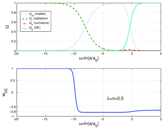
Figure 1: The evolutions of the energy densities $\Omega_{m}$, $\Omega_{r}$, $\Omega_{k}$ and $\Omega_{\phi}$ and the equation of state parameter $w_{\phi}$ of the quintessence field.

From figure 1, we see that DE dominates the Universe now and it has the correct equation of state to give the acceleration. By using the observational constraint, we also obtain the constraints on the parameters $\lambda$ and $n$ in figure 2. From figure 2, we see that the bigger $n$ is, the smaller $\lambda$ is allowed. This can be understood from equation (On curvature coupling and quintessence fine-tuning). If $\lambda$ is bigger, then $y^{\prime\prime}$ becomes more negative when the scalar field dominated the Universe. So $y^{\prime}$ decreases faster and takes more negative value. Therefore from equation (23), we see that $n$ must be smaller to satisfy the constraint of $w_{\phi}$.

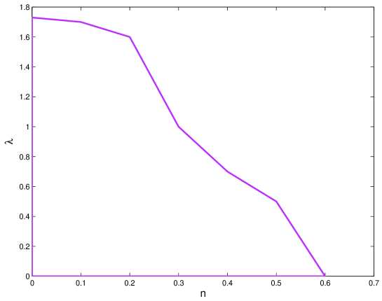
Figure 2: The allowed parameter space from observational constraints.

In summary, we analyze the curvature dependence model proposed by França which solves the fine-tuning problem of DE model. We find that the definitions of the energy density and pressure of the scalar field should be changed in order that the Klein-Gordon equation of the scalar field is equivalent to the energy conservation equation for the scalar field if the scalar field potential also depends on the scale factor. We then modify the curvature dependence of the quintessence potential from $k/a^{2}$ to $k/a^{n}$. In the phenomenological model in which the quintessence potential depends linearly on $k/a^{n}$ for $n\leq 0.6$, we find that the fine-tuning problem of the quintessence potential can be solved too. We would like to stress that the model is also a pure phenomenological one. The exact form of the non-minimal coupling of the scalar field to gravity is still unknown.

References

• [1] \NameBennett C. L. et al. \REVIEWAstrophys. J. Supp. Ser.14820031.
• [2] \NameRiess A. G. et al. \REVIEWAstrophys. J.6072004665.
• [3] \NameCaldwell R. R., Dave R. Steinhardt P. J. \REVIEWPhy. Rev. Lett.8019981582; \NameZlatev I., Wang L. Steinhardt P. J. \REVIEWPhy. Rev. Lett.821999896; \NameFerreira P. G. Joyce M. \REVIEWPhy. Rev. Lett.7919974740; \NameRatra B. and Peebles P. J. E. \REVIEWPhys. Rev. D3719883406; \NameWetterich C. \REVIEWNucl. Phys. B3021988668.
• [4] \NameCohen A., Kaplan D. Nelson A. \REVIEWPhys. Rev. Lett.8219994971; \NameHsu S. D. H. \REVIEWPhys. Lett. B594200413; \NameLi M. \REVIEWPhys. Lett. B60320041; \NameHuang Q. G. Gong Y. G. \REVIEWJCAP04082004006; \NameGong Y. G., Wang B. Zhang Y. Z. \REVIEWPhys. Rev. D722005043510.
• [5] \NamePavón D. Zimdahl W. \REVIEWPhys.Lett. B6282005206; \NameWang B., Gong Y. G. Abdalla E. \REVIEWPhys. Lett. B6242005141.
• [6] \NameSahni V. Starobinsky A. A. \REVIEWInt. J. Mod. Phys. D92000373; \NamePadmanabhan T. \REVIEWPhys. Rep.3802003235 ; \NamePeebles P. J. E. Ratra B. \REVIEWRev. Mod. Phys752003559; \NamePadmanabhan T. astro-ph/0510492.
• [7] \NameFreedman W. et al. \REVIEWAstrophys. J.553200147.
• [8] \NameFrança U. astro-ph/0509177.
• [9] \NameFrança U. astro-ph/0510692.
• [10] \NameGong Y. G. Zhang Y. Z. \REVIEWPhys. Rev. D722005043518; \NameLazkoz R., Nesseris S. Perivolaropoulos L. \REVIEWJCAP05112005010.