MPP-2005-122
LMU-ASC 68/05
hep-th/0510170 One in a Billion: MSSM-like D-Brane Statistics

Abstract

Continuing our recent work hep-th/0411173, we study the statistics of four-dimensional, supersymmetric intersecting D-brane models in a toroidal orientifold background. We have performed a vast computer survey of solutions to the stringy consistency conditions and present their statistical implications with special emphasis on the frequency of Standard Model features. Among the topics we discuss are the implications of the K-theory constraints, statistical correlations among physical quantities and an investigation of the various statistical suppression factors arising once certain Standard Model features are required. We estimate the frequency of an MSSM like gauge group with three generations to be one in a billion.

1 Introduction

The identification of MSSM-like string vacua is of obvious importance. Methods have been developed to study compactifications in various corners of the string respectively M-theory moduli space. The classes of models that have been discussed in most detail are certainly $E_{8}\times E_{8}$ heterotic string compactifications (e.g. [1, 2, 3]) and Type II orientifold models with intersecting/magnetised D-branes (for references we refer to the most recent review [4]).

Despite the enormous effort put into this study and the unquestionable successes in understanding the structure of these string models, we are still lacking a single fully realistic candidate. Models have been found which naturally give rise to certain features of the Standard Model, but all promising candidates have failed to be realistic at a certain step. Before getting too desperate about these shortcomings, though, one should keep in mind that the current search is restricted to very special corners of the overall configuration space, namely those which are technically under good control such as toroidal orbifolds or Gepner model orientifolds [5, 6, 7, 8]. A scan of all possible models is still far beyond the present state of the art. Therefore, the reason why no perfect model has been found yet might simply be that there are too many string vacua and that the, say, one million models encountered so far are only the tip of the iceberg of the enormous plethora of possible string vacua.

The existence of a very large number of string vacua has found convincing support recently by the study of flux vacua (for references see the review [9]). The fluxes induce a superpotential which allows to freeze the former moduli fields related to the size and shape of the underlying geometry. A rough estimate of the number of stable minima gave that there might exist of the order of $10^{500}$ string vacua. During the last two years, this huge number has triggered new ideas both on fine tuning problems in particle physics and cosmology and on the right approach towards the problem of identifying realistic string vacua. In [10] it was advocated that, complementary to the model by model search, a statistical approach to the string vacuum problem might be worthwhile to pursue. In fact such an analysis could reveal insights into the space of string vacua which might eventually provide some hints as to in which corner one should look for realistic models or may at least give us an estimate of the abundance of Standard-like models. We might even have to face the prospect that such a statistical analysis is the best we can ever do.

There exists a still growing collection of work dealing with the statistics of both Type II and M-theory flux compactifications. In these studies the statistical analysis is mostly concerned with the gravitational (closed string) sector of the vacua, see e.g. [11, 12, 13, 14, 15, 16, 17, 18, 19, 20, 21, 22, 23]. Comparatively little is known about the statistics in the gauge sector of the theory [26, 27, 8, 28, 29, 30, 31]. Of course these two sectors are not unrelated, as, like in Type II, many open string couplings also depend on the closed string moduli and therefore on the fluxes freezing them. Even more drastically, the closed sector back-reacts on the open string sector giving rise to supersymmetry breaking and induced soft-terms on the branes [32, 33, 34, 35, 36]. These are all phenomenologically very important and string theoretically very involved issues, which in a really complete statistical analysis have to be taken into account. However, practically such a thorough analysis is beyond our understanding of the theory and therefore has to wait until these points are better and more generally understood.

As in our first analysis [28], in this paper we follow a more modest approach and try to investigate for a quite well understood concrete example the statistical distributions of some of the main quantities of the gauge theory sector like the rank of the gauge group or the number of generations. More concretely, we study supersymmetric intersecting D-brane models on the $T^{6}\over Z_{2}\times Z_{2}$ orientifold background, which has enjoyed great interest in the past (see e.g. [37, 38, 39, 40, 41] among many others). We consider the ensemble of solutions to the tadpole cancellation conditions using a special class of supersymmetric, so-called ‘factorizable’, D-branes.

In general there will appear a D-term potential which contains scalar fields charged under the $U(1)$ gauge symmetry and Fayet-Iliopoulos terms depending on one half of the closed string moduli fields (complex structure moduli for Type IIA and Kähler moduli for T-dual Type IIB models). Therefore, at this level one expects to get a moduli space of vacua, parameterised by combinations of closed and open string scalars and containing regions with different gauge symmetry and chiral matter content. As a result, it is not so clear what one should actually count as a string vacuum. Our attitude is that we are not really counting different unconnected string moduli spaces but we are counting regions in the moduli space with different gauge groups.

Turning on a charged open string modulus corresponds geometrically to a recombination process of branes and therefore leads in general to curved objects outside our class of flat factorizable branes. On the other hand the inclusion of supersymmetric three-form fluxes (in the Type IIB picture) might lead to $\mu$-terms for some of the charged non-chiral fields and therefore freeze some of the open string moduli. It seems that the best we can do at the moment is to count solutions of the tadpole cancellation and K-theory conditions in the restricted set of supersymmetric branes one can actually describe. Since we are doing statistics we are confident that the distributions we find are relatively stable against the inclusion of a larger set of branes.

In [28] we have mainly used the saddle point method to derive the distributions and correlations of various physical quantities and for eight- and six-dimensional toy models we could confirm this technique against a brute force computer search. For the most interesting four-dimensional models the saddle point method also became more involved and time consuming and at the same time a brute force computer search could not be carried out in, say, a couple of weeks. Moreover, in [28] we had not taken the additional K-theory constraints [42] into account.

In this paper we report on the results of an extensive computer search involving several computer clusters looking for supersymmetric models which satisfy both the tadpole and the K-theory constraints. Using this large set of data we will statistically analyse the question: Among all these models, what is the percentage satisfying certain Standard Model requirements, like Standard Model or Pati-Salam gauge group, a massless hypercharge and three fermion generations?

The very special framework of open string models on which our analysis is based immediately raises a crucial question: How generic are our results in the complete moduli space of string theory? A trustworthy answer of this question can only be given by comparing the analysis of this article to analogous statistical results in corresponding corners of the landscape. In view of the current status in the systematic exploration of string vacua, progress seems difficult to make. As a very first step into this direction, we attempt a comparison of our large volume statistics and the small radius Gepner models of [8] wherever the two sets of data are compatible. In particular we distinguish between topological and geometrical observables and analyse how their distributions differ (or not).

The paper is organized as follows: Section 2 reviews the well known properties of the class of models we are considering. We give details about the tadpole, supersymmetry and K-theory constraints that arise in general and about the additional conditions we get from requiring Standard Model-like properties. In section 3 we explain the implementation of the problem in algorithmic form, suitable for a systematic computer analysis. Furthermore we address the issue of finiteness of the number of solutions. Section 4 contains the results of our computer search in form of statistical distributions, while in section 5 we analyse these distributions focusing on the correlation of variables. In section 6 we summarize our conclusions and give an outlook to further directions of research.

2 Model building ingredients

2.1 Parameterisation of Type II orientifolds

Orientifolds with magnetised D-branes are T-dual to orientifold models of intersecting D-branes. Although the inclusion of three-form fluxes is better understood in the Type IIB picture, the general models will be presented in the Type IIA picture with intersecting D6-branes, where many quantities have a geometrical interpretation at least for vanishing three-form flux. This is the case on which we concentrate in this work.

In the Type IIA language the orientifold action is taken to be $\Omega\bar{\sigma}$, where $\bar{\sigma}$ is an anti-holomorphic involution on the compact six-dimensional space preserving three-cycles $\Pi_{{\rm O}6}$. The R-R charge of the O6-planes has to be cancelled by a suitable set of stacks of $N_{a}$ D6-branes wrapping the three-cycles $\Pi_{a}$ and their $\Omega\bar{\sigma}$ images $\Pi^{\prime}_{a}$. The R-R tadpole cancellation condition can be written simply as

$$\sum_{a=1}^{k}N_{a}\,(\Pi_{a}+\Pi^{\prime}_{a})=4\,\Pi_{{\rm O}6}.$$ (1)

The homology group $H_{3}({\cal M})$ can be decomposed into its $\Omega\bar{\sigma}$ even and odd parts, $H_{3}({\cal M})=H^{+}_{3}({\cal M})\oplus H^{-}_{3}({\cal M})$. If $\alpha_{I}\in H^{+}_{3}({\cal M})$ and $\beta_{I}\in H^{-}_{3}({\cal M})$ form a symplectic basis, i.e. $\alpha_{I}\circ\beta_{J}=\delta_{IJ}$, $\alpha_{I}\circ\alpha_{J}=\beta_{I}\circ\beta_{J}=0$ with $I,J\in\{1,\ldots,h_{2,1}+1\}$, any cycle can be expanded as

$$\Pi_{a}=\vec{X_{a}}\vec{\alpha}+\vec{Y_{a}}\vec{\beta},\quad\Pi^{\prime}_{a}=\vec{X_{a}}\vec{\alpha}-\vec{Y_{a}}\vec{\beta},\quad\Pi_{{\rm O}6}={1\over 2}\vec{L}\vec{\alpha}.$$ (2)

Here $\vec{X_{a}}\vec{\alpha}\equiv\sum_{I=1}^{h_{2,1}+1}X_{a}^{I}\alpha_{I}$ and $X_{a}^{I}$, $Y_{a}^{I}$ are integer valued expansion coefficients.

The supersymmetry conditions read

$$\vec{Y_{a}}\vec{F}(U)=0,\quad\vec{X_{a}}\vec{U}>0,$$ (3)

where $U_{I}=\int_{\alpha_{I}}\Omega_{3}$ are the complex structure moduli and $F_{I}=\int_{\beta_{I}}\Omega_{3}$.

The intersection number between two cycles is given by

$$I_{ab}\equiv\Pi_{a}\circ\Pi_{b}=\vec{X_{a}}\vec{Y_{b}}-\vec{X_{b}}\vec{Y_{a}}.$$ (4)

The general chiral spectrum is computed from the intersection numbers as shown in table 1.

reps.	multiplicity	reps.	multiplicity
$({\bf N}_{a},\overline{{\bf N}}_{b})$	$I_{ab}$	${\bf Sym}_{a}$	$\frac{1}{2}(I_{aa^{\prime}}-I_{a{\rm O}6})$
$({\bf N}_{a},{\bf N}_{b})$	$I_{ab^{\prime}}$	${\bf Anti}_{a}$	$\frac{1}{2}(I_{aa^{\prime}}+I_{a{\rm O}6})$

Table 1: Multiplicities of the chiral spectrum from the intersection numbers.

2.2 Gauge anomalies and K-theory constraints

Using table 1 and  (4) one can compute that the cubic $SU(N_{a})$ gauge anomalies vanish if the tadpole cancellation condition (1) is satisfied.

Mixed abelian anomalies on the other hand do occur. The mixed gauge anomaly, for example, is of the form

$${\cal A}_{U(1)_{a}-SU(N_{b})^{2}} \sim N_{a}(I_{ab}+I_{ab^{\prime}})C_{2}(N_{b})$$ (5)

$$= -2N_{a}\vec{Y}_{a}\vec{X}_{b}C_{2}(N_{b})$$

up to terms which vanish upon tadpole cancellation. $C_{2}(N_{b})$ denotes the quadratic Casimir operator of the fundamental representation of $SU(N_{b})$.

A massless linear combination of abelian factors

$$U(1)_{massless}=\sum_{a}x_{a}U(1)_{a}$$ (6)

exists for

$$\sum_{a}x_{a}N_{a}\vec{Y}_{a}=0,$$ (7)

as can be easily seen from (5). More details can be found in [43].

Although the tadpole cancellation condition ensures the absence of cubic non-abelian gauge anomalies and mixed and cubic abelian gauge anomalies are cancelled by a generalized Green-Schwarz mechanism, there exists one further model building constraint [42] due to a $\mathbb{Z}_{2}$-valued conserved quantity, the K-theory charge. This quantity can be seen by introducing a probe $Sp(2)\simeq SU(2)$ brane. If the K-theory charge conservation is violated, there occurs a global gauge anomaly. This anomaly is manifest as the existence of an odd number of chiral fermions transforming in the fundamental representation of $Sp(2)$ [44].

2.3 The $T^{6}/({\mathbb{Z}}_{2}\times{\mathbb{Z}}_{2})$ model

Factorizable three-cycles in a toroidal background are parameterised by their wrapping number $(n_{i},m_{i})$, $i\in\{1,2,3\}$, along the basic one-cycles $(\pi_{2i-1},\pi_{2i})$ of $\prod_{i=1}^{3}T_{i}^{2}$. Two different shapes per two-torus $T_{i}^{2}$ respect the $\Omega\bar{\sigma}$ symmetry $z^{i}\rightarrow\bar{z}^{i}$ and they are parameterised by $b_{i}\in\{0,\frac{1}{2}\}$,

$$\Omega\bar{\sigma}:\pi_{2i-1}\rightarrow\pi_{2i-1}-2b_{i}\;\pi_{2i},\quad\quad\Omega\bar{\sigma}:\pi_{2i}\rightarrow-\pi_{2i}.$$ (8)

It is convenient to work with the $\Omega\bar{\sigma}$ even combination

$$\tilde{\pi}_{2i-1}=\pi_{2i-1}-b_{i}\pi_{2i},$$ (9)

because this modification does not change the computation of basic cycle intersection numbers (although only $\frac{1}{1-b_{i}}\,\tilde{\pi}_{2i-1}$ lies in the torus lattice).

The effective overall wrapping numbers of the three-cycles are conveniently parameterised by the integers

$$\hat{X}^{0} = \hat{b}n_{1}\,n_{2}\,n_{3},\quad\hat{Y}_{0}=\hat{b}\tilde{m}_{1}\,\tilde{m}_{2}\,\tilde{m}_{3},$$ (10)

$$\hat{X}^{i} = -\hat{b}n_{i}\,\tilde{m}_{j}\,\tilde{m}_{k},\quad\hat{Y}^{i}=-\hat{b}\tilde{m}_{i}n_{j}n_{k},\quad i,j,k\in\{1,2,3\}\;\mbox{cyclic},$$

where $\tilde{m}_{i}=m_{i}+b_{i}\,n_{i}$ is the effective wrapping number along $\tilde{\pi}_{2i-1}$ and $\hat{b}=[(1-b_{1})(1-b_{2})(1-b_{3})]^{-1}$. Observe that as in [28] we have included a minus sign in the definition of $\hat{X}_{i}$ and $\hat{Y}_{i}$ for $i=1,2,3$. Furthermore due to the overall scaling factor $\hat{b}$, which we introduce to obtain integer valued quantities also for tilted tori, the intersection numbers are computed from

$$I_{ab}=\hat{b}^{-2}\left(\hat{\vec{X}}_{a}\hat{\vec{Y}}_{b}-\hat{\vec{X}}_{b}\hat{\vec{Y}}_{a}\right).$$ (11)

In terms of these quantities, the supersymmetry condition reads

$$\sum_{I=0}^{3}\hat{Y}^{I}\frac{1}{U_{I}}=0,\quad\quad\sum_{I=0}^{3}\hat{X}^{I}U_{I}>0,$$ (12)

where the $U_{I}$ are defined in terms of the torus radii as

$$U_{0}=R^{(1)}_{1}R^{(2)}_{1}R^{(3)}_{1},\quad\quad U_{i}=R^{(i)}_{1}R^{(j)}_{2}R^{(k)}_{2},\quad i,j,k\in\{1,2,3\}\;\mbox{cyclic}.$$ (13)

The tadpole cancellation condition is given by

$$\sum_{a}N_{a}\hat{X}_{a}^{0} = 8\hat{b},$$

$$\sum_{a}N_{a}\hat{X}_{a}^{i} = \frac{8}{1-b_{i}},\quad i\in\{1,2,3\},$$ (14)

i.e. we have $\hat{\vec{L}}=L\,(\hat{b},(1-b_{i})^{-1})^{T}$ with $L=8$. The effective wrapping numbers can easily be rewritten in the original unscaled wrapping numbers along the basic three-cycles via the relations ($i,j,k\in\{1,2,3\}$ cyclic)

$$X^{0} = \hat{b}^{-1}\hat{X}^{0},$$

$$X^{i} = n_{i}m_{j}m_{k}=\hat{b}^{-1}\left(-\hat{X}^{i}+b_{j}\hat{Y}^{k}+b_{k}\hat{Y}^{j}+b_{j}b_{k}\hat{X}^{0}\right),$$

$$Y^{0} = m_{1}m_{2}m_{3}=\hat{b}^{-1}\left(\hat{Y}^{0}+\sum_{i=1}^{3}b_{i}\hat{X}^{i}-\sum_{i=1}^{3}b_{j}b_{k}\hat{Y}^{i}-b_{1}b_{2}b_{3}\hat{X}^{0}\right),$$

$$Y^{i} = m_{i}n_{j}n_{k}=\hat{b}^{-1}\left(-\hat{Y}^{i}-b_{i}\hat{X}^{0}\right).$$ (15)

These quantities are needed to implement the coprime condition on the sets $(n_{i},m_{i})$ of the wrapping numbers per two-torus,

$$(Y_{0})^{2}=\prod_{i=1}^{3}\gcd(Y_{0},X_{i}).$$ (16)

However, for computational convenience we will work with the rescaled wrapping numbers (10), which fulfill the same multiplicative relations as the original ones,

$$\hat{X}^{I}\hat{Y}^{I} = \hat{X}^{J}\hat{Y}^{J}\quad{\rm for}\;{\rm all}\;I,J\in\{0,\ldots,3\},$$ (17)

$$\hat{X}^{I}\hat{X}^{J} = -\hat{Y}^{K}\hat{Y}^{L},\quad\hat{X}^{L}(\hat{Y}^{L})^{2}=-\hat{X}^{I}\hat{X}^{J}\hat{X}^{K},\quad\hat{Y}^{L}(\hat{X}^{L})^{2}=-\hat{Y}^{I}\hat{Y}^{J}\hat{Y}^{K},$$

where on the second line $I,J,K,L$ are permutations of $\{0,\ldots,3\}$.

The number of chiral (anti)symmetric representations of some $U(N_{a})$ factor is given in table 1. If one imposes for phenomenological reasons the constraint $\#({\rm Sym}_{a})=0$, this leads to $\#({\rm Anti}_{a})=-\frac{8}{\hat{b}^{2}}\hat{X}_{a}^{0}\hat{Y}_{a}^{0}$ and one can distinguish two cases:

1. $\#({\rm Anti}_{a})=\#({\rm Sym}_{a})=0$, where for some permutation $(I,J,K,L)$ of $(0,\ldots,3)$ we have the relations on supersymmetric factorizable branes

   $$\hat{Y}^{I}_{a}=\hat{Y}^{J}_{a}=\hat{X}^{K}_{a}=\hat{X}^{L}_{a}=0, \quad\quad\hat{X}^{I}_{a}\hat{X}^{J}_{a}=-\hat{Y}^{K}_{a}\hat{Y}^{L}_{a}\neq 0,$$

   $$\hat{Y}^{K}_{a}\hat{L}^{K}+\hat{Y}^{L}_{a}\hat{L}^{L}=0, \quad\hat{L}^{K}U^{K}=\hat{L}^{L}U^{L}.$$ (18)

   These are the types of branes occurring also in compactifications to six dimensions as explained in [28].

2. $\#({\rm Anti}_{a})\neq 0,\#({\rm Sym}_{a})=0$: in this case $\hat{X}^{I}_{a}\neq 0$ for all $I\in\{0,\ldots,3\}$ and the constraint on the vanishing net number of chiral symmetric representations can be rephrased as

   $$\sum_{I=0}^{3}\frac{1}{\hat{X}^{I}_{a}}\hat{L}^{I}=16,$$ (19)

   while (12) has to be fulfilled.

The D-brane configurations discussed so far support $U(N_{a})$ gauge factors. In addition, there exist four different kinds of $Sp(N_{b})$ gauge factors, each of them descending from branes wrapping the $\Omega\bar{\sigma}\theta^{k}\omega^{l}$ ($k,l\in\{0,1\}$) invariant planes, where $\theta$ and $\omega$ are the two orbifold generators. The wrapping numbers of these branes are ($i,j,k\in\{1,2,3\}$ cyclic)

$$\hat{X}^{0} = \hat{b}^{2},\;\;\hat{X}^{1}=\hat{X}^{2}=\hat{X}^{3}=0\qquad{\rm or}\qquad\hat{X}^{i}=\frac{\hat{b}}{1-b_{i}},\;\;\hat{X}^{0}=\hat{X}^{j}=\hat{X}^{k}=0,$$

$$\hat{Y}^{I} = 0\quad{\rm for}\;{\rm all}\;I.$$ (20)

The K-theory constraints on consistent chiral spectra demand that there must be an even number of chiral fermions transforming in the fundamental representation of any possible $Sp(2)$ factor. Inserting the wrapping numbers of all four $Sp(2)$ candidates into (11) and summing over all $U(N_{a})$ factors, the K-theory constraints take the form

$$\sum_{a}N_{a}\hat{Y}^{0}_{a} \in 2\mathbb{Z},$$

$$(1-b_{j})(1-b_{k})\sum_{a}N_{a}\hat{Y}^{i}_{a} \in 2\mathbb{Z},\quad i,j,k\in\{1,2,3\}\;\mbox{cyclic}.$$ (21)

2.4 Standard Model realisations

particle		mult.
$U(3)_{a}\times Sp(2)_{b}\times U(1)_{c}\times U(1)_{d}$ with $Q_{Y}^{(S)}$
$Q_{L}$	$({\bf 3},{\bf 2})_{0,0}$	$I_{ab}$
$u_{R}$	$(\overline{{\bf 3}},1)_{-1,0}+(\overline{{\bf 3}},1)_{0,-1}$	$I_{a^{\prime}c}+I_{a^{\prime}d}$
$d_{R}$	$(\overline{{\bf 3}},1)_{1,0}+(\overline{{\bf 3}},1)_{0,1}$	$I_{a^{\prime}c^{\prime}}+I_{a^{\prime}d^{\prime}}$
$d_{R}$	$(\overline{{\bf 3}}_{A},1)_{0,0}$	$\frac{1}{2}(I_{aa^{\prime}}+I_{a{\rm O}6})$
$L$	$(1,{\bf 2})_{-1,0}+(1,{\bf 2})_{0,-1}$	$I_{bc}+I_{bd}$
$e_{R}$	$({\bf 1},{\bf 1})_{2,0}$	$\frac{1}{2}(I_{cc^{\prime}}-I_{c{\rm O}6})$
$e_{R}$	$({\bf 1},{\bf 1})_{0,2}$	$\frac{1}{2}(I_{dd^{\prime}}-I_{d{\rm O}6})$
$e_{R}$	$({\bf 1},{\bf 1})_{1,1}$	$I_{cd^{\prime}}$
$U(3)_{a}\times U(2)_{b}\times U(1)_{c}\times U(1)_{d}$ with $Q_{Y}^{(S)}$
$Q_{L}$	$({\bf 3},\overline{{\bf 2}})_{0,0}$	$I_{ab}$
$Q_{L}$	$({\bf 3},{\bf 2})_{0,0}$	$I_{ab^{\prime}}$
$u_{R}$	$(\overline{{\bf 3}},1)_{-1,0}+(\overline{{\bf 3}},1)_{0,-1}$	$I_{a^{\prime}c}+I_{a^{\prime}d}$
$d_{R}$	$(\overline{{\bf 3}},1)_{1,0}+(\overline{{\bf 3}},1)_{0,1}$	$I_{a^{\prime}c^{\prime}}+I_{a^{\prime}d^{\prime}}$
$d_{R}$	$(\overline{{\bf 3}}_{A},1)_{0,0}$	$\frac{1}{2}(I_{aa^{\prime}}+I_{a{\rm O}6})$
$L$	$(1,{\bf 2})_{-1,0}+(1,{\bf 2})_{0,-1}$	$I_{bc}+I_{bd}$
$L$	$(1,\overline{{\bf 2}})_{-1,0}+(1,\overline{{\bf 2}})_{0,-1}$	$I_{b^{\prime}c}+I_{b^{\prime}d}$
$e_{R}$	$({\bf 1},{\bf 1})_{2,0}$	$\frac{1}{2}(I_{cc^{\prime}}-I_{c{\rm O}6})$
$e_{R}$	$({\bf 1},{\bf 1})_{0,2}$	$\frac{1}{2}(I_{dd^{\prime}}-I_{d{\rm O}6})$
$e_{R}$	$({\bf 1},{\bf 1})_{1,1}$	$I_{cd^{\prime}}$

Table 2: Realisation of quarks and leptons for various hypercharges. Part 1.

particle		mult.
$U(3)_{a}\times U(2)_{b}\times U(1)_{c}\times U(1)_{d}$ with $Q_{Y}^{(1)}$
$Q_{L}$	$({\bf 3},\overline{{\bf 2}})_{0,0}$	$I_{ab}$
$u_{R}$	$(\overline{{\bf 3}}_{A},1)_{0,0}$	$\frac{1}{2}(I_{aa^{\prime}}+I_{a{\rm O}6})$
$d_{R}$	$(\overline{{\bf 3}},1)_{-1,0}+(\overline{{\bf 3}},1)_{0,-1}$	$I_{a^{\prime}c}+I_{a^{\prime}d}$
$d_{R}$	$(\overline{{\bf 3}},1)_{1,0}+(\overline{{\bf 3}},1)_{0,1}$	$I_{a^{\prime}c^{\prime}}+I_{a^{\prime}d^{\prime}}$
$L$	$(1,{\bf 2})_{-1,0}+(1,{\bf 2})_{0,-1}$	$I_{bc}+I_{bd}$
$L$	$(1,{\bf 2})_{1,0}+(1,{\bf 2})_{0,1}$	$I_{bc^{\prime}}+I_{bd^{\prime}}$
$e_{R}$	$({\bf 1},\overline{{\bf 1}}_{A})_{0,0}$	$-\frac{1}{2}(I_{bb^{\prime}}+I_{b{\rm O}6})$
$U(3)_{a}\times U(2)_{b}\times U(1)_{c}\times U(1)_{d}$ with $Q_{Y}^{(2)}$
$Q_{L}$	$({\bf 3},\overline{{\bf 2}})_{0,0}$	$I_{ab}$
$u_{R}$	$(\overline{{\bf 3}}_{A},1)_{0,0}$	$\frac{1}{2}(I_{aa^{\prime}}+I_{a{\rm O}6})$
$d_{R}$	$(\overline{{\bf 3}},1)_{-1,0}$	$I_{a^{\prime}c}$
$d_{R}$	$(\overline{{\bf 3}},1)_{1,0}$	$I_{a^{\prime}c^{\prime}}$
$L$	$(1,\overline{{\bf 2}})_{0,-1}$	$I_{b^{\prime}d}$
$e_{R}$	$({\bf 1},\overline{{\bf 1}}_{A})_{0,0}$	$-\frac{1}{2}(I_{bb^{\prime}}+I_{b{\rm O}6})$
$e_{R}$	$({\bf 1},{\bf 1})_{1,1}$	$I_{cd^{\prime}}$
$e_{R}$	$({\bf 1},{\bf 1})_{-1,1}$	$I_{c^{\prime}d^{\prime}}$

Table 3: Realisation of quarks and leptons for various hypercharges. Part 2.

For a Standard Model like sector of $\chi$ quark and lepton generations in a four stack intersecting D-brane model, the gauge group has to contain one of the two following factors

1. $U(3)_{a}\times Sp(2)_{b}\times U(1)_{c}\times U(1)_{d}$

2. $U(3)_{a}\times U(2)_{b}\times U(1)_{c}\times U(1)_{d}$

with $\#({\rm Sym}_{a})=\#({\rm Sym}_{b})=0$ in order to have no exotic symmetric chiral matter of the two non-abelian factors. The first stack is therefore of the type (18) or (19), the second can also be of the form (20). In some cases, the Standard Model quantum numbers can also be realised on three stacks only at the cost of having no standard Yukawa couplings (which are not always realistic in the four stack models either).

Up to an interchange of cycles and their $\Omega\bar{\sigma}$ images, there exist three different possible definitions of the hypercharge for quarks and left-handed leptons:

1. The ‘standard’ definition $Q_{Y}^{(S)}=\frac{1}{6}Q_{a}+\frac{1}{2}Q_{c}+\frac{1}{2}Q_{d}$, valid for both choices of an $Sp(2)_{b}$ or $U(2)_{b}$ factor. This hypercharge is massless if $\hat{\vec{Y}}_{a}+\hat{\vec{Y}}_{c}+\hat{\vec{Y}}_{d}=0$.

2. The first ‘non-standard’ definition $Q_{Y}^{(1)}=-\frac{1}{3}Q_{a}-\frac{1}{2}Q_{b}$, where right-handed up-type quarks are realised as antisymmetric representations of $U(3)_{a}$ [45, 46]. In order for this hypercharge candidate to be massless, $\hat{\vec{Y}}_{a}+\hat{\vec{Y}}_{b}=0$ has to be satisfied.

3. The second ‘non-standard’ definition $Q_{Y}^{(2)}=-\frac{1}{3}Q_{a}-\frac{1}{2}Q_{b}+Q_{d}$, where again right-handed up-type quarks are realised as antisymmetric representations of $U(3)_{a}$. $\hat{\vec{Y}}_{a}+\hat{\vec{Y}}_{b}-\hat{\vec{Y}}_{d}=0$ is the condition for this abelian factor to remain massless.

The ‘standard’ definition of the hypercharge on four stacks admits the realisation of all Standard Model particles as bifundamental representations, thereby ensuring the existence of Yukawa couplings from triangles of three intersecting branes. This case can be reduced to a three stack model by simply replacing $\frac{1}{2}(Q_{c}+Q_{d})\rightarrow\frac{1}{2}Q_{c}$.

The first ‘non-standard’ definition also has a direct reduction to three stacks since $Q_{c}$ and $Q_{d}$ do not appear in the definition of $Q_{Y}^{(1)}$. On the other hand, the second ‘non-standard’ definition really requires four stacks of branes.

The corresponding realisations of the Standard Model quarks and leptons are given in tables 2 and 3. Apart from the listed particles, there exist candidates for right handed neutrinos and Higgs multiplets for each possible hypercharge.

Having $\chi_{Q}$ generations of quarks amounts for the first case to setting

$$\chi_{Q}=I_{ab}=I_{a^{\prime}c}+I_{a^{\prime}d}=I_{a^{\prime}c^{\prime}}+I_{a^{\prime}d^{\prime}}+\frac{1}{2}(I_{aa^{\prime}}+I_{a{\rm O}6})$$ (22)

and $\chi_{L}$ lepton generations occur for

$$\chi_{L}=I_{bc}+I_{bd}=\frac{1}{2}(I_{cc^{\prime}}-I_{c{\rm O}6})+\frac{1}{2}(I_{dd^{\prime}}-I_{d{\rm O}6})+I_{cd^{\prime}}.$$ (23)

For the remaining cases, the analogous formulae can be read off from tables 2 and 3.

3 Computer algorithms

We have defined the wrapping numbers $\hat{X}^{I}$ and $\hat{Y}^{I}$ as integer valued quantities in order to implement the supersymmetry (12) and tadpole (2.3) conditions in a fast computer algorithm. From the equations we can derive the following inequalities

$$0<\sum_{I=0}^{3}\hat{X}^{I}\,{U}_{I}\leq\sum_{I=0}^{3}\hat{L}^{I}\,{U}_{I}.$$ (24)

In a first step possible values for the wrapping numbers $\hat{X}^{I}$ and $\hat{Y}^{I}$ are computed using (24) for a fixed set of complex structures.

In a second step we use the tadpole equations (2.3), which after summation can be reduced to

$$\sum_{a}S_{a}=C\quad\mbox{with}\quad S_{a}=\sum_{I}N_{a}{U}_{I}\hat{X}_{a}^{I}\quad\mbox{and}\quad C=\sum_{I}\hat{L}^{I}{U}_{I}.$$ (25)

The algorithm to find solutions to these equations computes all possible partitions of $C$ and factorises them into possible values for $N_{a}$ and $\hat{X}_{a}^{I}$, taking only factorizations into account which match the values generated in the first step. The results obtained in this way have to be checked again if they satisfy all consistency conditions, especially the K-theory constraints.

3.1 Number of solutions

It is an important question whether or not the number of solutions is infinite, because a statistical statement can only be of significance if we are dealing with a finite set of models. Unfortunately we have not been able to give a complete analytic proof of finiteness of the considered space of models, but we have good numerical hints towards this assumption.

As explained in [28], it is sufficient to analyse the possible configurations of wrapping numbers for models in which all $\hat{X}^{I}$ are non-vanishing. The tadpole equations can then be shown to admit only a finite number of supersymmetric configurations for a fixed choice of rational complex structures and fixed $L$. The difficult question is which complex structures are compatible with the consistency conditions. For toroidal compactifications to six dimensions it is possible to give an upper bound for the complex structures in terms of $L$. In the four-dimensional case, however, it is not immediately clear how to achieve this. Figure 2 shows how the total number of mutually different brane configurations for $L=2$ increases and saturates, as we include more and more combinations of values for the complex structures $U_{I}$ into the set for which we construct solutions. For this small toy value of $L$ our algorithm actually admits pushing the computations up to those complex structures where obviously no additional brane solutions exist.

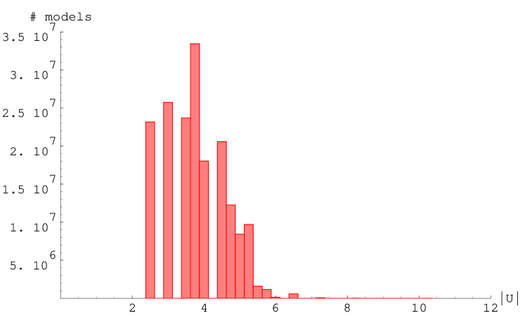
Figure 1: The number of different configurations of $\hat{X}^{I}$ for $L=2$, satisfying the constraints. The x-axis shows combinations of complex structures in an arbitrary scale.

Figure 2: The number of models for $L=8$, plotted against the absolute value of $\vec{U}$. The highest analysed value of $\vec{U}$ is 12.

For the physically relevant case of $L=8$ the total number of models compared to the absolute value $|\vec{U}|$ of the complex structure variables scales as displayed in figure 2. The plot shows all complex structures we have actually been able to analyse systematically. We find that the number of solutions falls logarithmically for increasing values of $|\vec{U}|$. In order to interpret this result, we observe that the complex structure moduli $U_{I}$ are only defined up to an overall rescaling by the volume modulus of the compact space. We have chosen all radii and thereby also all $U_{I}$ to be integer valued, which means that large $|\vec{U}|$ correspond to large coprime values of $R_{1}^{(i)}$ and $R_{2}^{(i)}$. This comprises on the one hand decompactification limits which have to be discarded in any case for phenomenological reasons, but on the other hand also tori which are slightly distorted from e.g. square tori for $R_{2}^{(i)}/R_{1}^{(i)}=0.99$.

Combining the results of the two numerical tests we have reason to hope that we can indeed make a convincing statistical statement using the analysed data. Nevertheless, at this point it should be mentioned that we cannot fully exclude that a large number of new solutions appears at those values for the complex structures which we have not analysed.

3.2 Complexity

The main problem of the algorithm used to compute the models lies in the fact that its complexity scales exponentially with the complex structure parameters. Therefore we are not able to compute up to arbitrarily high values for the $U_{I}$. Although we tried our best, it may of course be possible to improve the algorithm in many ways, but unfortunately the exponential behaviour cannot be cured unless we might have access to a quantum computer. This is due to the fact that the problem of finding solutions to the diophantine equations we are considering falls in the class of NP complete problems [47], which means that they cannot be reduced to problems which are solvable in polynomial time. In fact, this is quite a severe issue since the diophantine structure of the tadpole equations encountered here is not at all exceptional but very generic for the topological constraints also in other types of string constructions.

For the total number of models analysed in this paper, which is around $1.66\times 10^{8}$, we used several computer clusters built out of standard PCs with an approximative total CPU time of roughly $4\times 10^{5}$ hours. To estimate how many models could be computed in principle using a computer grid equipped with contemporary technology in a reasonable amount of time, the exponential behaviour of the problem has to be taken into account. Let us be optimistic and imagine that we would have a total number of $10^{5}$ processors at our disposal which are twice as fast as the ones we have been using. Expanding our analysis to cover a range of complex structures which is twice as large as the one we considered would in a very rough estimate still take us of the order of 500 years.

Note that in principle there can be a big difference in the estimated computing time for the two computational problems of finding all string vacua in a certain class and of singling out special realistic ones. Apparently, for the second question, having Standard Model features realized by just a subset or even a single stack of branes, the search algorithm can work recursively by successively imposing more Standard Model features. It would be interesting to know whether the Standard Model search can be performed by an algorithm which is polynomial.

4 Statistical distributions

4.1 Effect of the K-theory constraints

(a) Rank distribution

(b) $U(M)$ distribution

Figure 3: Probability distributions for $L=8,U_{I}=1$. The stars represent the distribution without K-theory constraints, the boxes give the result including the constraints.

Using the explicit constructions obtained by the computer algorithm, it is possible to quantify the effect of imposing the K-theory constraints (2.3). The overall effect of the additional constraints is to suppress the number of possible brane configurations by a factor of five. For example in the case without flux considered in this article, i.e. $L=8$, and for complex structures $U_{I}=1\forall I$ and non-tilted tori, we get approximatively $1.3\times 10^{8}$ models if we do not impose the constraints and ca. $2.3\times 10^{7}$ models enforcing them.

Because the distribution of models is highly dominated by configurations where the value for $\hat{Y}^{I}$ is 0 or 1 (in agreement with the observation that only $1.6\%$ of all models live on tilted tori), one expects that the constraints of equation (2.3) suppress models with odd total rank. This is indeed the case as can be seen in figure 3(a). Note that the distribution shown is limited to the case of all complex structures chosen as $U_{I}=1$, but different values of the complex structure change only the maximum and width of the distribution, not its shape, which is therefore generic.

By contrast, other observables are more or less unaffected by the inclusion of K-theory constraints, for example the frequency of models containing at least one gauge group $U(M)$, as shown in figure 3(b) (as above the distribution for one specific value of the complex structures is generic). This is due to the fact that the constraints do not limit the individual brane configurations but only the overall composition of them to form a consistent model. In both cases the supersymmetric brane configurations are dominated by stacks of a small number $N_{a}$ of branes.

Let us compare the overall suppression of models by the K-theory constraints to the analogous results for Gepner Models [26, 48]. Unfortunately, a direct comparison of our gauge statistics and the Gepner Model data is not possible, since the abundance of solutions at the Gepner point forced the authors to restrict their search a priori to Standard Model like vacua. The effects of implementing also the above K-theory constraints for this class of vacua are analysed in [48], resulting only in a practically negligible suppression factor. The discrepancy is even more striking if one considers that the number of symplectic branes and therefore of additional K-theory constraints in many, though not in all of the Gepner orientifolds is much higher than on our toroidal orbifold. However, the MSSM-like models analysed on the Gepner side satisfy very strong constraints, in particular the $U(1)_{Y}$ massless condition (cf. equation (7)). We have reason to infer that these requirements a priori rule out most of those models which violate the K-theory constraints.

4.2 Correlations between the total rank of the gauge group and chirality

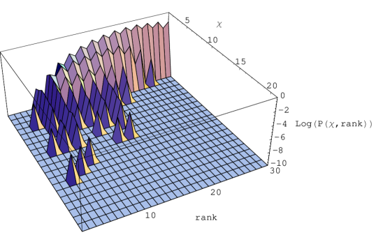
(a) with K-theory constraints

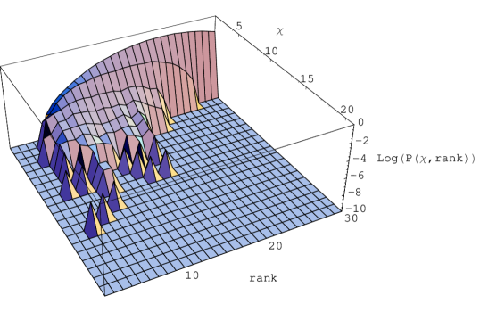
(b) without K-theory constraints

Figure 4: The frequency distribution of models of specific rank and chirality. $L=8,U_{I}=1$.

We find a correlation between the rank of the gauge group and the mean chirality of the model, which we have defined as

$$\chi=<I_{a^{\prime}b}-I_{ab}>=\hat{b}^{-2}<2\hat{\vec{Y}}_{a}\hat{\vec{X}}_{b}>=\frac{2}{k(k-1)}\sum_{\stackrel{{\scriptstyle a,b\in\{1,..,k\}}}{{b<a}}}\hat{b}^{-2}\hat{\vec{Y}}_{a}\hat{\vec{X}}_{b}.$$ (26)

In this respect the explicit computer search confirms the results obtained via a saddle point approximation in [28].

As can be seen in figure 4, the K-theory constraints do not change the overall shape of the distribution except for a suppression of models with odd total rank, as already seen in figure 3(a).

4.3 Statistics of Standard-like models

An analysis of the possible realizations of models with MSSM-like features, as described in section 2.4, shows a surprising result: We do not encounter any three-generation Standard Model in our analysis. As displayed in figure 5(a) the only configurations we have found exhibit one, two or four generations, with a strong statistical domination of the one-generation models.

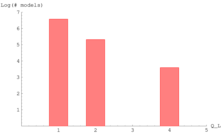
(a) MSSM models

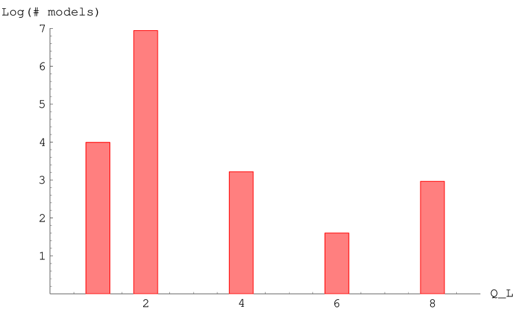
(b) Pati-Salam models

Figure 5: Logarithmic plot of the number of models versus the number of generations.

Given the fact that models with three generations have been constructed explicitly in our setup (see e.g.[49, 50]) this might appear as an incorrect result at first sight. The important point to notice here is that all three-generation models known to us share the property that they need values for the complex structures which in our conventions are very large and out of the reach of our computer analysis. Another issue not to be neglected is that most of the models considered in the literature make use of some special features like brane recombination, brane splitting (breaking of higher rank gauge groups) etc. From this observation and the arguments in section 3.1 we might draw the conclusion that three-generation models are statistically very highly suppressed in this specific orbifold setup.

4.4 Massless hypercharge

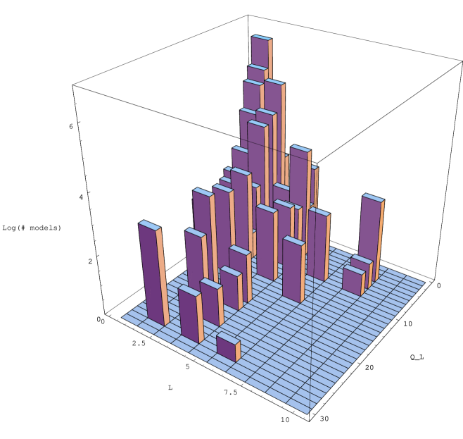
Figure 6: Logarithmic plot of the number of models with Standard Model characteristics, not including the condition for a massless hypercharge, depending on the number of generations in the quark ($Q_{L}$) and lepton ($L$) sector.

To gain some further insight into the distribution of Standard Model-like properties, we have performed an analysis of our models that includes all constraints for MSSM-like models except for the condition of having a massless hypercharge $U(1)_{Y}$. Furthermore we allow for a different number of generations in the quark and lepton sector. The resulting distribution for different numbers of quark and lepton generations in shown in figure 6.

From the phenomenological point of view these models are of course not extremely useful because the massless $U(1)_{Y}$ condition is important for a consistent MSSM structure, but the result is nevertheless quite interesting, as it turns out that even within this relaxed framework no three generation model can be found. The closest we can get to a three-generation model is a configuration with three generations of quarks and four lepton generations.

4.5 Pati-Salam models

In addition to the direct realisation of MSSM models we also analysed the occurrence of models with a Pati-Salam gauge group

$$SU(4)\times SU(2)_{L}\times SU(2)_{R}.$$ (27)

As can be seen in figure 5(b), we get one-, two-, four-, six- and eight-generation models, but again no model with three generations. Also in this case there exist explicit constructions of three-generation Standard Models in the literature [50] and our conclusions are the same as in section 4.3 - the statistical suppression of three generation models is extremely large.

4.6 Statistics of the hidden sector

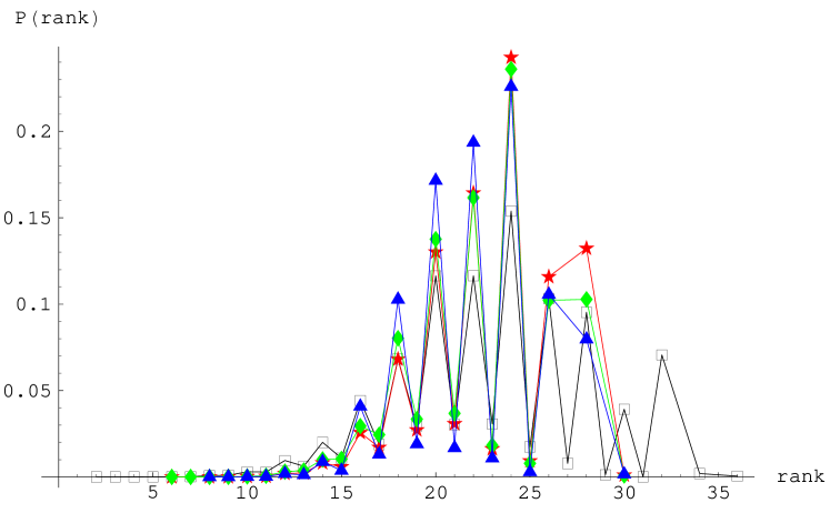
(a) Rank distribution

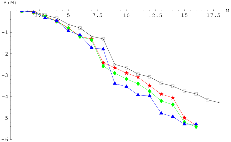
(b) $U(M)$ distribution

Figure 7: Frequency distributions of all models (empty black boxes) and in the hidden sector of MSSM models (red stars), MSSM models without restriction to a massless $U(1)$ (green diamonds) and Pati-Salam models (blue triangles).

An interesting question in a statistical context concerns the properties of the hidden sector of our models. In figures 7(a) and 7(b) the distribution of the total rank of the gauge group and the frequency of models containing a $U(M)$ gauge factor in the hidden sector are compared with the results one obtains from an analysis of all models considered.

As it turns out the distributions of the constrained models differ only very little from those of the full set. The small deviations which are visible in the plots cannot be regarded as indications of fundamentally different behaviour. They must be seen rather as a remnant of the statistical analysis, which looses its applicability in the region of very high rank of the gauge groups where the number of models is very small as compared to the region of lower rank.

This suggests that the statistical distributions are not affected by the additional constraints of requiring a specific configuration in the visible sector. This observation gives some hints about the correlation of variables, which will be explored in greater detail in the section 5.

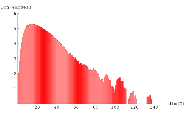
(a) Full set of models

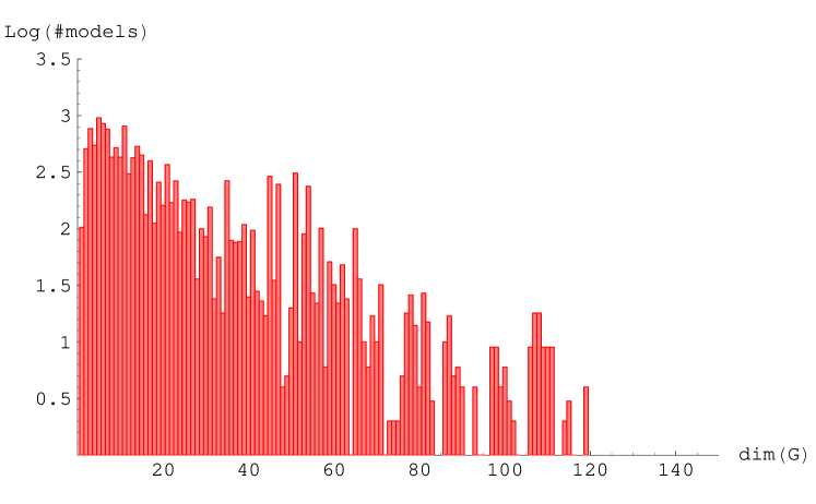
(b) Restricted set with max. three branes in the hidden sector

Figure 8: Logarithmic plots of the number of models with Standard Model gauge group and massless $U(1)$ depending on the dimension of the gauge group G in the hidden sector.

A comparison of the distribution of the total dimension of the gauge group in the hidden sector of Standard Model-like configurations with the results for Gepner models in [8] shows two quite similar pictures. In figure 8(a) we give the complete distribution, in 8(b) we allow for maximally three branes in the hidden sector in order to make the result better comparable to [8], where a similar cutoff was imposed for computational reasons. The main difference comes from the fact that we have much fewer models in our ensemble and, more importantly, our models are not constrained to three generations.

4.7 Gauge couplings

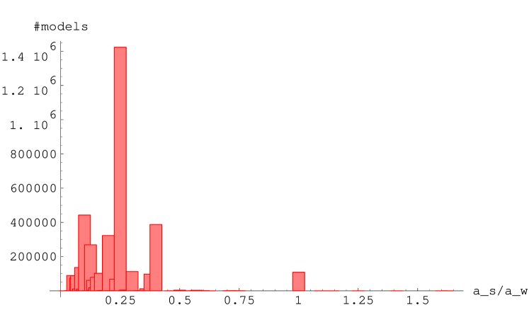
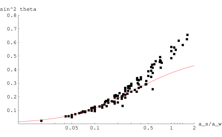
Figure 9: Distribution of $\frac{\alpha_{s}}{\alpha_{w}}$ in Standard Model-like configurations.

Figure 10: Values of $sin^{2}\theta$ depending on $\frac{\alpha_{s}}{\alpha_{w}}$ (on a logarithmic scale). Each dot represents a class of models with these values. The red line shows the relation (28), which is satisfied for $88\%$ of all models

The observables considered so far all belong only to the topological sector of the model in that they are defined by the wrapping numbers of the branes and manifestly independent of the geometric moduli of the compactification manifold. A quantity which is relatively easy to analyse but which does contain geometrical information are the gauge couplings in the visible sector. In [51] it was argued that a MSSM model built with intersecting branes naturally leads to a relation between the coupling constants,

$$\frac{1}{\alpha_{Y}}=\frac{2}{3}\frac{1}{\alpha_{s}}+\frac{1}{\alpha_{w}},$$ (28)

where $\alpha_{Y/s/w}$ are the couplings of the hypercharge, the strong and weak sector respectively. Note that this relation of the coupling constants does not imply that these models automatically exhibit full gauge unification, but it could fit into an $SU(5)$ framework.

For an honest check of this relation we would have to use the renormalization group equations and evolve the coupling constants from the string scale down to their low energy values. In our analysis we have not done so, but investigated instead the relation between the couplings at the string scale. Therefore we can only get some hints towards the actual relation at lower scales.

To calculate the gauge couplings we use the expression derived in [51] for the gauge coupling of a stack $a$ in an intersecting brane model, which reads in our conventions

$$\frac{1}{\alpha_{a}}=\frac{c}{\kappa_{a}}\,\frac{1}{\hat{b}\sqrt{\prod_{i=1}^{3}R_{1}^{(i)}R_{2}^{(i)}}}\sum_{I=0}^{3}\hat{X}^{I}U_{I}.$$ (29)

The constant $c$ is given by

$$c=\frac{1}{2\sqrt{2}}\frac{M_{Planck}}{M_{s}}$$ (30)

and $\kappa_{a}$ is 1 for an $U(N)$ stack and 2 for a $SO(2N)$ or $Sp(2N)$ stack. Note the explicit dependence on the complex structures.

For the coupling of the hypercharge $\alpha_{Y}$, we have to consider the contribution from all stacks of branes in the visible sector and distinguish the three different possibilities we consider for a MSSM configuration, as explained in section 2.4. Using

$$\frac{1}{\alpha_{Y}}=\sum_{i}2N_{i}x_{i}^{2}\frac{1}{\alpha_{i}},$$ (31)

we get for the three configurations

$$\frac{1}{\alpha_{Y}}=\left\{\begin{array}[]{rl}1.&\displaystyle\frac{1}{6}\frac{1}{\alpha_{a}}+\frac{1}{2}\frac{1}{\alpha_{c}}+\frac{1}{2}\frac{1}{\alpha_{d}},\\[8.61108pt] 2.&\displaystyle\frac{2}{3}\frac{1}{\alpha_{a}}+\frac{1}{\alpha_{b}},\\[8.61108pt] 3.&\displaystyle\frac{2}{3}\frac{1}{\alpha_{a}}+\frac{1}{\alpha_{b}}+2\frac{1}{\alpha_{d}}.\end{array}\right.$$ (32)

In figure 10 the distribution of the ratio $\alpha_{s}$ to $\alpha_{w}$ is displayed. We find that only for 2.75% of all models $\alpha_{s}=\alpha_{w}$ at the string scale and that the weak coupling constant is generically larger than the strong one.

Figure 10 shows the different values for $\sin^{2}\theta$, depending on the ratio of $\alpha_{s}/\alpha_{w}$. The red line represents the ratio given in (28). $\sin^{2}\theta$ is calculated from

$$\sin^{2}\theta=\frac{\alpha_{Y}}{\alpha_{Y}+\alpha_{w}}.$$ (33)

We find that 88% of the models obey the relation (28). Note that this result might be a bit obscured by the plot because it shows one dot for every possible value, not taking into account that there exist many models with exactly the same values. In fact there exist many more models with low values for $\alpha_{s}/\alpha_{w}$ and $\sin^{2}\theta$, which happen to be the ones fulfilling the relation.

These results can also be compared with the analysis of [8], where as in the case of the hidden gauge group one has to take into account that we are dealing with a smaller ensemble and with models that are not constrained to exactly three generations of fermions. The fraction of MSSM-like Gepner models satisfying (28) is found there to be only ca. $10\%$. Without wanting to over-interpret this mismatch, we emphasize once more that the gauge couplings are not part of the topological sector of the theory and that therefore deviations between the small and large radius regime fit into the general picture.

5 Correlations

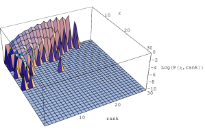
(a) MSSM-like models

(b) MSSM-like models with massive $U(1)$

(c) Pati-Salam models

Figure 11: The relative frequency to find models of specific rank and chirality, requiring different visible sectors to be present in the models.

(a) $\scriptstyle P_{c}=|P(3)*P(2/Sp2)-P(2/Sp2\wedge 3)|/C$

(b) $\scriptstyle P_{c}=|P(3)*P(ns)-P(3_{ns})|/C$

Figure 12: Correlations between atomic properties of MSSM-like configurations. The factor $C$ is a normalization, see equation (34). Relative frequencies are labeled as follows: $P(M)$: frequency of stacks with gauge group $U(M)$; $P(2/Sp2)$: frequency of $U(2)$ or $Sp(2)$ stacks; $P(ns)$: frequency of gauge groups without symmetric representations.

In this section we investigate the correlation between different observables in greater detail. As analysed in section 4.6, the statistics of the hidden sector of MSSM-like and Pati-Salam models are, on a statistical basis, very similar to the full statistics of all models. The same is also true for the non-trivial correlations between observables in our models. This is shown in figure 11 for the example of the correlation between mean chirality and total rank of the gauge group, as discussed in section 4.2.

Putting these hints together we might conclude that the ‘atomic’ frequency distributions actually do not depend on the specific kind of models chosen (e.g. MSSM-like, Pati-Salam or something else), but only on a generic distribution which is already present in the completely unconstrained setup.

To make this statement more quantitative, we calculate the frequencies for some atomic properties important for model building. In particular, we check whether two properties $A$ and $B$ are statistically independent in the ensemble of D-brane models. A good measure for statistical dependence is given by

$$P_{AB}=\frac{P(A)\times P(B)-P(A\wedge B)}{P(A)\times P(B)+P(A\wedge B)}.$$ (34)

As properties we choose the appearance of models with at least one $U(3)$ or $U(2)/Sp(2)$ gauge factors or with at least one stack without symmetric representations.

The results are presented in figure 12 depending on the number of stacks of the models under consideration. Note that the frequency of finding $U(1)$ stacks is close to one and therefore does not lead to any further suppression for the appearance of a MSSM like model. The plots demonstrate that, for sufficiently large numbers of stacks, the considered properties are statistically independent and that therefore their frequencies simply multiply. Note that this was an assumption in the statistical estimates carried out in the original work [10]. The combined values (integrated over all models) for the correlation between the properties of an MSSM-like model (without restriction to massless $U(1)_{Y}$) is 0.094, which is reasonably low to justify considering the individual properties as essentially independent.

5.1 Estimate of three generation Standard Models

Having found that the constraints are statistically only very little correlated we can make some predictions about the overall probability of configurations in our setup which do not show up in the data like for example true Standard Models. In table 4 we summarize the factors coming from the various constraints. The two $U(1)$ gauge groups required for our Standard Model setup are not included, because, as mentioned, the frequency of having one of them is essentially one. In addition we give the fraction of models - among all configurations containing a $U(3)\times U(2)$ factor without symmetric representations - which meet in addition the individual constraints of a massless hypercharge, of three generations of quarks or of three lepton families.

Restriction	Factor
gauge factor $U(3)$	$0.0816$
gauge factor $U(2)/Sp(2)$	$0.992$
No symmetric representations	$0.839$
Massless $U(1)_{Y}$	$0.423$
Three generations of quarks	$2.92\times 10^{-5}$
Three generations of leptons	$1.62\times 10^{-3}$
Total	$1.3\times 10^{-9}$

Table 4: Suppression factors for various constraints of Standard Model properties.

Multiplying all these factors leads to an overall suppression factor of

$$R\approx\,1.3\times 10^{-9},$$ (35)

i.e. only one in a billion models gives rise to a four stack D-brane vacuum with Standard Model gauge symmetry and three generations of quark and leptons. Multiplying this with the total number of models analysed, $N\approx\,1.66\times 10^{8}$, leaves us with 0.21 true Standard Models in our ensemble.

5.2 How good is this estimate?

To get some idea about the quality of this estimate we can apply the method used for three generation models to Standard Model-like solutions we actually did find in our analysis. The result of this computation for two and four family models is given in table 5. This check clearly shows that our estimate gives the right order of magnitude of the number of expected solutions, but the precise value might differ by several standard deviations.

# generations	# of models found	estimated #	suppression factor
$2$	$162921$	$188908$	$\approx 10^{-3}$
$3$	$0$	$0.2$	$\approx 10^{-9}$
$4$	$3898$	$3310$	$\approx 2\times 10^{-5}$

Table 5: Comparison between the estimated number of solutions and the actual number of solutions found for models with two, three and four generations.

6 Conclusions

In this work we have given an explicit statistical analysis of the vacuum structure in a specific example of Type II orientifold models. The bottom line is that a Standard Model-like configuration with three families of quarks and leptons in this class of models is statistically highly suppressed. The concrete models which have so far been constructed in this setup can therefore be regarded as exceptional within the vast majority of possible solutions. The same holds also for models with a Pati-Salam gauge group.

A statistical analysis of the different observables shows that there exist non-trivial correlations between some of them such as the rank of the gauge group and the chirality of the models. Interestingly, these correlations hardly depend on whether we analyse them in the full set of solutions or only in the hidden sector of some specific visible configuration. In that respect, the hidden sectors of a Standard Model or Pati-Salam construction exhibit universal behavior and we expect this to hold for any other visible sector as long as the number of constraints it imposes is comparable.

Despite this general occurrence of correlations, we can quantitatively justify the hypothesis that the basic properties of Standard Model-like constructions are to sufficiently good accuracy independent. Under this assumption, we derive an estimate for the relative frequency of three-generation Standard Models in our setup which is of the order of $10^{-9}$. Of course, by requiring more of the phenomenological features of the Standard Model such as Yukawa couplings, gauge couplings, soft supersymmetry breaking terms, the occurrence of realistic models will get further reduced. However, these properties really depend on the finer details of the models (see for instance [52, 53, 54, 55]) and an honest statistical treatment of them is much harder to carry out.

An important question is how generic our results actually are. Even though the available data for both frameworks are only partially compatible, we have performed a rough comparison with the statistics of the hidden sector of MSSM-like Gepner model orientifolds [26] where possible. The geometrical properties of these small radius constructions differ considerably from those of the large radius regime. However, the results seem to suggest that the observables of the topological sector exhibit quite similar distributions. This is not so surprising as the diophantine structure of the consistency conditions describing this sector is essentially the same for both frameworks and since, after all, topological quantities should be protected against too drastic changes as one varies the coupling constants or radii. In fact, we regard this as strong hints towards a universal behaviour in the distribution of the topological observables also in other string constructions. By contrast, the distribution of the gauge couplings, which are dependent on the geometric moduli of the theory, do differ. It would be very desirable to collect more evidence supporting this picture.

For this purpose it is important to study the statistics of other quite well understood classes of models like for instance heterotic string compactifications on elliptically fibered Calabi-Yau manifolds (see for instance [56, 3, 57, 58]). Questions in this direction include: Does the distribution of the rank of the gauge group qualitatively have the same shape? What is the abundance of Standard like models? In addition, as we started to investigate in our first paper [28], it would be interesting to combine the T-dual picture of magnetised branes with additional three-form fluxes [59, 60, 49, 61] and determine the effect on the statistics.

Acknowledgements

It is a pleasure to acknowledge interesting discussions with Bobby Acharya, Mirjam Cvetič, Frederik Denef, Michael Douglas and Gary Shiu.

We would like to thank the Max-Planck-Rechenzentrum in Garching and the system administrators at the Max-Planck-Institut für Physik for technical support.

References

- [1] L. E. Ibanez, J. E. Kim, H. P. Nilles, and F. Quevedo, “Orbifold compactifications with three families of su(3) x su(2) x u(1)**n,” Phys. Lett. B191 (1987) 282–286.
- [2] J. A. Casas and C. Munoz, “Three generation su(3) x su(2) x u(1)-y models from orbifolds,” Phys. Lett. B214 (1988) 63.
- [3] V. Braun, Y.-H. He, B. A. Ovrut, and T. Pantev, “A heterotic standard model,” hep-th/0501070.
- [4] R. Blumenhagen, M. Cvetic, P. Langacker, and G. Shiu, “Toward realistic intersecting d-brane models,” hep-th/0502005.
- [5] R. Blumenhagen and A. Wisskirchen, “Spectra of 4d, n=1 type i string vacua on non-toroidal cy threefolds,” Phys. Lett. B438 (1998) 52–60, hep-th/9806131.
- [6] I. Brunner, K. Hori, K. Hosomichi, and J. Walcher, “Orientifolds of gepner models,” hep-th/0401137.
- [7] R. Blumenhagen and T. Weigand, “Chiral supersymmetric gepner model orientifolds,” JHEP 02 (2004) 041, hep-th/0401148.
- [8] T. P. T. Dijkstra, L. R. Huiszoon, and A. N. Schellekens, “Supersymmetric standard model spectra from rcft orientifolds,” Nucl. Phys. B710 (2005) 3–57, hep-th/0411129.
- [9] M. Grana, “Flux compactifications in string theory: A comprehensive review,” hep-th/0509003.
- [10] M. R. Douglas, “The statistics of string / m theory vacua,” JHEP 05 (2003) 046, hep-th/0303194.
- [11] S. Ashok and M. R. Douglas, “Counting flux vacua,” JHEP 01 (2004) 060, hep-th/0307049.
- [12] F. Denef and M. R. Douglas, “Distributions of flux vacua,” JHEP 05 (2004) 072, hep-th/0404116.
- [13] A. Giryavets, S. Kachru, and P. K. Tripathy, “On the taxonomy of flux vacua,” JHEP 08 (2004) 002, hep-th/0404243.
- [14] M. Dine, E. Gorbatov, and S. D. Thomas, “Low energy supersymmetry from the landscape,” hep-th/0407043.
- [15] A. Misra and A. Nanda, “Flux vacua statistics for two-parameter calabi-yau’s,” Fortsch. Phys. 53 (2005) 246–259, hep-th/0407252.
- [16] J. P. Conlon and F. Quevedo, “On the explicit construction and statistics of calabi-yau flux vacua,” JHEP 10 (2004) 039, hep-th/0409215.
- [17] F. Denef and M. R. Douglas, “Distributions of nonsupersymmetric flux vacua,” JHEP 03 (2005) 061, hep-th/0411183.
- [18] O. DeWolfe, A. Giryavets, S. Kachru, and W. Taylor, “Enumerating flux vacua with enhanced symmetries,” JHEP 02 (2005) 037, hep-th/0411061.
- [19] K. R. Dienes, E. Dudas, and T. Gherghetta, “A calculable toy model of the landscape,” hep-th/0412185.
- [20] M. Dine, D. O’Neil, and Z. Sun, “Branches of the landscape,” JHEP 07 (2005) 014, hep-th/0501214.
- [21] B. S. Acharya, F. Denef, and R. Valandro, “Statistics of m theory vacua,” hep-th/0502060.
- [22] J. Distler and U. Varadarajan, “Random polynomials and the friendly landscape,” hep-th/0507090.
- [23] M. R. Douglas and Z. Lu, “Finiteness of volume of moduli spaces,” hep-th/0509224.
- [24] T. Banks, M. Dine, and E. Gorbatov, “Is there a string theory landscape?,” JHEP 08 (2004) 058, hep-th/0309170.
- [25] T. Banks, “Landskepticism or why effective potentials don’t count string models,” hep-th/0412129.
- [26] T. P. T. Dijkstra, L. R. Huiszoon, and A. N. Schellekens, “Chiral supersymmetric standard model spectra from orientifolds of gepner models,” Phys. Lett. B609 (2005) 408–417, hep-th/0403196.
- [27] J. Kumar and J. D. Wells, “Landscape cartography: A coarse survey of gauge group rank and stabilization of the proton,” Phys. Rev. D71 (2005) 026009, hep-th/0409218.
- [28] R. Blumenhagen, F. Gmeiner, G. Honecker, D. Lüst, and T. Weigand, “The statistics of supersymmetric d-brane models,” Nucl. Phys. B713 (2005) 83–135, hep-th/0411173.
- [29] J. Kumar and J. D. Wells, “Surveying standard model flux vacua on t**6/z(2) x z(2),” hep-th/0506252.
- [30] N. Arkani-Hamed, S. Dimopoulos, and S. Kachru, “Predictive landscapes and new physics at a tev,” hep-th/0501082.
- [31] C. Vafa, “The string landscape and the swampland,” hep-th/0509212.
- [32] P. G. Cámara, L. E. Ibáñez, and A. M. Uranga, “Flux-induced susy-breaking soft terms,” Nucl. Phys. B689 (2004) 195–242, hep-th/0311241.
- [33] M. Grana, T. W. Grimm, H. Jockers, and J. Louis, “Soft supersymmetry breaking in calabi-yau orientifolds with d-branes and fluxes,” Nucl. Phys. B690 (2004) 21–61, hep-th/0312232.
- [34] D. Lüst, S. Reffert, and S. Stieberger, “Flux-induced soft supersymmetry breaking in chiral type iib orientifolds with d3/d7-branes,” Nucl. Phys. B706 (2005) 3–52, hep-th/0406092.
- [35] D. Lüst, S. Reffert, and S. Stieberger, “Mssm with soft susy breaking terms from d7-branes with fluxes,” hep-th/0410074.
- [36] D. Lüst, P. Mayr, S. Reffert, and S. Stieberger, “F-theory flux, destabilization of orientifolds and soft terms on d7-branes,” hep-th/0501139.
- [37] S. Förste, G. Honecker, and R. Schreyer, “Supersymmetric z(n) x z(m) orientifolds in 4d with d-branes at angles,” Nucl. Phys. B593 (2001) 127–154, hep-th/0008250.
- [38] M. Cvetic, G. Shiu, and A. M. Uranga, “Chiral four-dimensional n = 1 supersymmetric type iia orientifolds from intersecting d6-branes,” Nucl. Phys. B615 (2001) 3–32, hep-th/0107166.
- [39] M. Larosa and G. Pradisi, “Magnetized four-dimensional z(2) x z(2) orientifolds,” Nucl. Phys. B667 (2003) 261–309, hep-th/0305224.
- [40] E. Dudas and C. Timirgaziu, “Internal magnetic fields and supersymmetry in orientifolds,” Nucl. Phys. B716 (2005) 65–87, hep-th/0502085.
- [41] R. Blumenhagen, M. Cvetic, F. Marchesano, and G. Shiu, “Chiral d-brane models with frozen open string moduli,” JHEP 03 (2005) 050, hep-th/0502095.
- [42] A. M. Uranga, “D-brane probes, rr tadpole cancellation and k-theory charge,” Nucl. Phys. B598 (2001) 225–246, hep-th/0011048.
- [43] L. E. Ibanez, F. Marchesano, and R. Rabadan, “Getting just the standard model at intersecting branes,” JHEP 11 (2001) 002, hep-th/0105155.
- [44] E. Witten, “An su(2) anomaly,” Phys. Lett. B117 (1982) 324–328.
- [45] I. Antoniadis, E. Kiritsis, and T. N. Tomaras, “A d-brane alternative to unification,” Phys. Lett. B486 (2000) 186–193, hep-ph/0004214.
- [46] R. Blumenhagen, B. Körs, D. Lüst, and T. Ott, “The standard model from stable intersecting brane world orbifolds,” Nucl. Phys. B616 (2001) 3–33, hep-th/0107138.
- [47] M. R. Garey and D. S. Johnson, Computers and Intractability, a Guide to the Theory of NP-Completeness. Freeman San Francisco, 1979.
- [48] B. Gato-Rivera and A. N. Schellekens, “Remarks on global anomalies in rcft orientifolds,” hep-th/0510074.
- [49] F. Marchesano and G. Shiu, “Building mssm flux vacua,” JHEP 11 (2004) 041, hep-th/0409132.
- [50] M. Cvetic, T. Li, and T. Liu, “Standard-like models as type iib flux vacua,” Phys. Rev. D71 (2005) 106008, hep-th/0501041.
- [51] R. Blumenhagen, D. Lüst, and S. Stieberger, “Gauge unification in supersymmetric intersecting brane worlds,” JHEP 07 (2003) 036, hep-th/0305146.
- [52] D. Cremades, L. E. Ibáñez, and F. Marchesano, “Yukawa couplings in intersecting d-brane models,” JHEP 07 (2003) 038, hep-th/0302105.
- [53] M. Cvetic and I. Papadimitriou, “Conformal field theory couplings for intersecting d-branes on orientifolds,” Phys. Rev. D68 (2003) 046001, hep-th/0303083.
- [54] S. A. Abel and A. W. Owen, “Interactions in intersecting brane models,” Nucl. Phys. B663 (2003) 197–214, hep-th/0303124.
- [55] G. L. Kane, P. Kumar, J. D. Lykken, and T. T. Wang, “Some phenomenology of intersecting d-brane models,” Phys. Rev. D71 (2005) 115017, hep-ph/0411125.
- [56] R. Friedman, J. Morgan, and E. Witten, “Vector bundles and f theory,” Commun. Math. Phys. 187 (1997) 679–743, hep-th/9701162.
- [57] R. Blumenhagen, G. Honecker, and T. Weigand, “Non-abelian brane worlds: The heterotic string story,” hep-th/0510049.
- [58] V. Braun, Y.-H. He, B. A. Ovrut, and T. Pantev, “Moduli dependent mu-terms in a heterotic standard model,” hep-th/0510142.
- [59] R. Blumenhagen, D. Lüst, and T. R. Taylor, “Moduli stabilization in chiral type iib orientifold models with fluxes,” Nucl. Phys. B663 (2003) 319–342, hep-th/0303016.
- [60] J. F. G. Cascales and A. M. Uranga, “Chiral 4d n = 1 string vacua with d-branes and nsns and rr fluxes,” JHEP 05 (2003) 011, hep-th/0303024.
- [61] J. Gomis, F. Marchesano, and D. Mateos, “An open string landscape,” hep-th/0506179.