SLAC-PUB-11532 Adaptive Perturbation Theory: Quantum Mechanics and Field Theory

Abstract

Adaptive perturbation is a new method for perturbatively computing the eigenvalues and eigenstates of quantum mechanical Hamiltonians that are widely believed not to be solvable by such methods[1]. The novel feature of adaptive perturbation theory is that it decomposes a given Hamiltonian, $H$, into an unperturbed part and a perturbation in a way which extracts the leading non-perturbative behavior of the problem exactly. In this talk I will introduce the method in the context of the pure anharmonic oscillator and then apply it to the case of tunneling between symmetric minima. After that, I will show how this method can be applied to field theory. In that discussion I will show how one can non-perturbatively extract the structure of mass, wavefunction and coupling constant renormalization.

1 Introduction

To avoid controversy I have titled this talk Adaptive Perturbation Theory, but I could have equally well called it Non-Perturbative Perturbation Theory (except that I was told people would dismiss it as crazy). Actually I hope you will agree by the end of the talk that such a title would have been eminently defensible.

2 Two Topics

This talk is divided into two parts. First I introduce the general ideas within the framework of ordinary quantum mechanics. Next, I show how to extend these ideas to the case of scalar field theory in any number of space-time dimensions. I will begin the quantum mechanics discussion by talking about the pure anharmonic oscillator and then extend this discussion to cover the anharmonic oscillator with either a positive or negative mass term.

The theory of an anharmonic oscillator with a positive mass term has a rich literature. The various authors usually attempt to resum the ordinary perturbation expansion to obtain the non-perturbative behavior. I will show that one can avoid such complication by exhibiting a convergent perturbation expansion for each eigenstate of the Hamiltonian. An expansion that, moveover, captures all non-perturbative features of the problem in zeroth order. The case of the anharmonic oscillator with a negative mass term will allow me to extend the simplest adaptive technique to handle the case of tunneling between symmetric minima. In this talk I will not discuss the case of tunneling between very asymmetric minima, however this topic is covered in the paper to appear on this work.

3 The Harmonic Oscillator

Let me begin by reminding you of a some simple facts pertaining to the ordinary harmonic oscillator. The Hamiltonian of the ordinary harmonic oscillator is:

$$H=\frac{1}{2m}\,p^{2}+\frac{m\omega^{2}}{2}\,x^{2},\quad{\rm where}\,\,\left[p,x\right]=-i.$$ (1)

Next, let me introduce $\gamma$-dependent operators ${A^{{\dagger}}_{\gamma}}$ and ${A_{\gamma}}$ by

$$x = {1\over\sqrt{2\gamma}}\left({A^{{\dagger}}_{\gamma}}+{A_{\gamma}}\right),$$

$$p = i\,\sqrt{\gamma\over 2}\left({A^{{\dagger}}_{\gamma}}-{A_{\gamma}}\right).$$ (2)

Substituting this into Eq. 1 yields

$$H = \frac{\gamma}{4\,m}\left(-{{A^{{\dagger}}_{\gamma}}}^{2}-{A_{\gamma}}^{2}+2\,{A^{{\dagger}}_{\gamma}}{A_{\gamma}}+1\right)$$ (3)

$$+ \frac{m\,\omega^{2}}{4\,\gamma}\left({{A^{{\dagger}}_{\gamma}}}^{2}+{A_{\gamma}}^{2}+2\,{A^{{\dagger}}_{\gamma}}{A_{\gamma}}+1\right).$$

It is customary to choose $\gamma=m\,\omega$ so as to cancel the terms ${{A^{{\dagger}}_{\gamma}}}^{2}$ and ${{A_{\gamma}}}^{2}$ and render the Hamiltonian diagonal in the number operator. This immediately tells us that the eigenstates of the Hamiltonian are the eigenstates of the number operator and that the energies of these states are given by $E_{n}=(n+1/2)\,\omega$.

4 The Anharmonic Oscillator

In the case of the general anharmonic oscillator the Hamiltonian is

$$H=\frac{1}{2}\,p^{2}+\frac{m\,\omega^{2}}{2}\,x^{2}+\frac{1}{6}\,\lambda\,x^{4}.$$ (4)

The customary way to deal with this problem is two introduce annihilation and creation operators chosen to diagonalize the first two terms and then construct a perturbation theory based upon expanding in the coupling $\lambda$. This approach has a well known problem; namely, it is known to diverge, no matter how small $\lambda$, due to $n!$ growth of the perturbation series. I will now show how to avoid this problem and produce a rapidly convergent adaptive perturbation theory expansion for each eigenstate and eigenvalue of $H$. To emphasize that this is not an expansion in $\lambda$ I will begin by specializing to the case $m=0$.

Setting $m=0$ in Eq. 4 and making the substitution for $x$ and $p$ given in Eq. 2, leads to

$$H=\frac{\gamma}{4} \hskip-18.0pt\left(-{A^{{\dagger}}_{\gamma}}^{2}-{A_{\gamma}}^{2}+2\,{A^{{\dagger}}_{\gamma}}{A_{\gamma}}+1\right)$$

$$+\frac{\lambda}{4\gamma^{2}} \hskip-18.0pt\left({A^{{\dagger}}_{\gamma}}^{2}{A_{\gamma}}^{2}+2{A^{{\dagger}}_{\gamma}}{A_{\gamma}}+1+\frac{1}{6}({A^{{\dagger}}_{\gamma}}^{4}+{A_{\gamma}}^{4})\right.$$

$$+\frac{2}{3}\left(\right. \hskip-18.0pt\left.{A^{{\dagger}}_{\gamma}}^{3}{A_{\gamma}}+{A^{{\dagger}}_{\gamma}}{A_{\gamma}}^{3})+({A^{{\dagger}}_{\gamma}}^{2}+{A_{\gamma}}^{2})\right)$$

$$=\left(\frac{\gamma}{4}\right. \hskip-18.0pt+\left.\frac{\lambda}{4\gamma^{2}}\right)(2\,{N_{\gamma}}+1)+\frac{\lambda}{4\gamma^{2}}{N_{\gamma}}\,({N_{\gamma}}-1)$$

$$+\left(\frac{\gamma}{4}\right. \hskip-18.0pt\left.-\frac{\lambda}{2\gamma^{2}}\right)({A^{{\dagger}}_{\gamma}}^{2}+{A_{\gamma}}^{2})$$

$$+\frac{\lambda}{4\gamma^{2}} \hskip-18.0pt\left(\frac{1}{6}({A^{{\dagger}}_{\gamma}}^{4}+{A_{\gamma}}^{4})+\frac{2}{3}({A^{{\dagger}}_{\gamma}}^{3}{A_{\gamma}}+{A^{{\dagger}}_{\gamma}}{A_{\gamma}}^{3})\right),$$

where I have defined the $\gamma$-dependent number operator

$${N_{\gamma}}={A^{{\dagger}}_{\gamma}}{A_{\gamma}}.$$ (6)

Given this expression I define the $\gamma$-dependent unperturbed Hamiltonian, $H_{0}$ and the perturbation $V$ by

$$H= \hskip-18.0ptH_{0}(\gamma)+V(\gamma),$$

$$H_{0}(\gamma)= \hskip-18.0pt\left(\frac{\gamma}{4}+\frac{\lambda}{4\gamma^{2}}\right)(2\,{N_{\gamma}}+1)+\frac{\lambda{N_{\gamma}}({N_{\gamma}}-1)}{4\gamma^{2}},$$

$$V(\gamma)= \hskip-18.0pt\left(\frac{\gamma}{4}-\frac{\lambda}{2\gamma^{2}}\right)({A^{{\dagger}}_{\gamma}}^{2}+{A_{\gamma}}^{2})$$

$$+\frac{\lambda}{4\gamma^{2}}\left(\frac{1}{6}\right. \hskip-18.0pt\left.({A^{{\dagger}}_{\gamma}}^{4}+{A_{\gamma}}^{4})+\frac{2}{3}({A^{{\dagger}}_{\gamma}}^{3}{A_{\gamma}}+{A^{{\dagger}}_{\gamma}}{A_{\gamma}}^{3})\right).$$

Now, since I have a different perturbation theory defined for each choice of $\gamma$, I need a principle for fixing $\gamma$. This is where the adaptive comes into adaptive perturbation theory. The key notion is that I will use a simple variational calculation, adapted to the eigenvalue to be calculated, in order to pick that value of $\gamma$ that gives the most convergent perturbation expansion.

To set up this variational calculation I first define a $\gamma$-dependent family of Fock-states, $|{N_{\gamma}}\rangle$. The $\gamma$-dependent vacuum state, $|0_{\gamma}\rangle$, is defined by the condition

$${A_{\gamma}}|0_{\gamma}\rangle=0,$$ (8)

and the $\gamma$-dependent $n$-particle state, i.e., the state for which

$$N_{\gamma}|{n_{\gamma}}\rangle=n|{n_{\gamma}}\rangle,$$ (9)

is just

$$|{n_{\gamma}}\rangle=\frac{1}{\sqrt{n!}}\,{A^{{\dagger}}_{\gamma}}^{n}|0_{\gamma}\rangle.$$ (10)

The value of $\gamma$ used to define the adaptive perturbation theory for the $n^{th}$ level of the anharmonic oscillator is determined by requiring that it minimize the expectation value

$$E_{n}(\gamma)=\langle{n_{\gamma}}|H|{n_{\gamma}}\rangle.$$ (11)

Eqs. 4-LABEL:pertdecomplast show that this expectation value is equal to

$$E_{n}(\gamma)\hskip-8.0pt = \hskip-8.0pt\langle{n_{\gamma}}|H_{0}(\gamma)|{n_{\gamma}}\rangle=\left(\frac{\gamma}{4}+\frac{\lambda}{4\gamma^{2}}\right)(2\,n+1)$$ (12)

$$+ \frac{\lambda}{4\gamma^{2}}n\,(n-1).$$

Minimizing $E_{n}(\gamma)$ with respect to $\gamma$ gives

$$\gamma=\lambda^{1/3}\left(\frac{2\,(n^{2}+n+1)}{2n+1}\right)^{1/3}.$$ (13)

At this point I substitute this value into Eq. 11 to obtain

$$E_{n}(\gamma)_{\rm min}\hskip-8.0pt = \hskip-8.0pt\frac{3}{8}\,\lambda^{1/3}\left(2n+1\right)^{2/3}\left(2n^{2}+2(n+1)\right)^{1/3}$$

which, for large $n$, behaves as $\lambda^{1/3}\,n^{4/3}$ , which is the correct answer.

The fact that all energies scale as $\lambda^{1/3}$ is an easily obtained exact result and so, the non-trivial part of variational computation is the derivation of the dependence of the energy on $n$. To see why all energies are proportional to $\lambda^{1/3}$ it suffices to make the following canonical transformation

$$x\rightarrow\frac{x}{\lambda^{1/6}}\quad;\quad p\rightarrow\lambda^{1/6}p.$$ (15)

In terms of these operators, the Hamiltonian of the pure anharmonic oscillator becomes

Table 1: A comparison of the zeroth order and second order perturbation results, for the energy of the $n^{th}$ level of the pure anharmonic oscillator, to the exact answer for $\lambda=1$ and widely varying values of $n$.

$\lambda$	$n$	Variational	$2^{nd}$ Order Perturbation	Exact	Variational % Err	Perturbative % Error
1.0	0	0.375	0.3712	0.3676	0.02	0.0098
1.0	1	1.334	1.3195	1.3173	0.01	0.0017
1.0	10	17.257	17.508	17.4228	-0.009	0.0049
1.0	40	104.317	105.888	105.360	-0.009	0.0050

$$H=\lambda^{1/3}\left(\frac{1}{2}p^{2}+\frac{1}{6}x^{4}\right),$$ (16)

thus proving the claim. A comparison of the variational computation and the result of a second-order perturbation theory for $\lambda=1$ and widely differing values of $n$ is given in Table 1. As advertised, we see that the adaptive perturbation theory for each level converges rapidly, independent of $\lambda$ and $n$.

Obviously, the same method can be used to study the case where $m^{2}>0$, except that now one has to solve a cubic equation to determine $\gamma$ as a function of $\lambda$,$m^{2}$ and $n$. The general result that for each $n$, second order perturbation theory is accurate to better than one percent still holds true.

4.1 What does this have to do with quasi-particles?

An interesting corollary to the adaptive perturbation theory technique is that it provides an explicit realization of the quasi-particle picture underlying much of many-body theory. What we have shown is that no matter how large the underlying coupling, the physics of the states near a given $n_{0}$-particle state can be accurately described in terms of perturbatively coupled eigenstates of an appropriately chosen harmonic oscillator. Of course, as we have seen, the appropriately chosen harmonic oscillator picture changes as $n_{0}$ changes. Furthermore, the perturbatively coupled states $|n_{\gamma(n_{0})}\rangle$, for $n\approx n_{0}$, correspond to states containing an infinite number of particles, if we choose as a basis those states that correspond to a significantly different value of $n_{0}$.

5 The Double Well

The most general negative mass version of the anharmonic oscillator can, up to an irrelevant constant, be written as:

$$H=\frac{1}{2}\,p^{2}+\frac{1}{6}\,\lambda\,\left(x^{2}-f^{2}\right)^{2}.$$ (17)

Clearly, for a non-vanishing value of $f^{2}$, this potential has two minima located at $x=\pm f$. Thus, we would expect that the best gaussian approximation to the ground state of this system can’t be a gaussian centered at the origin; classical intuition would imply that it is a gaussian centered about another point, $x=c$. In other words, if $|0_{\gamma}\rangle$ is a state centered at $x=0$, it is better to adopt a trial state of the form

$$|c,\gamma\rangle=e^{-icp}\,|0_{\gamma}\rangle.$$ (18)

Since

$$e^{icp}\,x\,e^{-icp}=x+c,$$ (19)

computing the expectation value of the Hamiltonian, Eq. 17, in the state specified in Eq. 18, is the same as computing the expectation value of the Hamiltonian obtained by replacing the operator $x$ by $x+c$, in the state $|0_{\gamma}\rangle$. In the language of the previous sections, this is equivalent to introducing the annihilation and creation operators ${A^{{\dagger}}_{\gamma}}$ and ${A_{\gamma}}$ as follows:

$$x = {1\over\sqrt{2\gamma}}\left({A^{{\dagger}}_{\gamma}}+{A_{\gamma}}\right)+c,$$

$$p = i\,\sqrt{\gamma\over 2}\left({A^{{\dagger}}_{\gamma}}-{A_{\gamma}}\right).$$ (20)

The expectation value of this Hamiltonian in the state $|0_{\gamma}\rangle$ is

$${\cal E}(c,\gamma) = \left(\frac{\gamma}{4}+\frac{\lambda f^{4}}{6}-\frac{\lambda f^{2}c^{2}}{3}+\frac{\lambda c^{4}}{6}+\frac{\lambda c^{2}}{2\gamma}\right.$$ (21)

$$+ \left.\frac{\lambda}{8\gamma^{2}}-\frac{\lambda f^{2}}{6\gamma}\right),$$

which should be minimized with respect to both $\gamma$ and $c$ in order to define the starting point of the adaptive perturbation theory computation.

To see what these equations tell us, it is convenient to hold $c$ fixed and solve for the value of $\gamma$ that minimizes ${\cal E}(\gamma,c)$; call this $\gamma(c)$, and then plot ${\cal E}(\gamma(c),c)$ for various values of $\lambda$ and $f^{2}$. Three such plots are shown in Fig. 1. The first plot is for a value of $f$ which is large enough so that the lowest energy is obtained for a gaussian shifted either to the right or left by the amount $c=\pm c_{\rm min}$. While there is a local minimum at $c=0$ it has a higher energy than the shifted states. Things change as one lowers the value of $f$. Thus, the second plot shows that for lower $f$ the shifted wavefunctions and the one centered at zero are essentially degenerate in energy. For a slightly smaller value of $f$ things reverse and the unshifted wavefunction has a lower energy than the shifted ones.

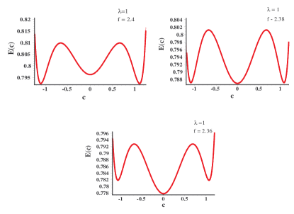
Figure 1: Effective potential as a function of $c$, showing two degenerate local minima at $c=\pm c_{\rm min}$ and one minimum at $c=0$. The three plots are for $\lambda=1$ and different values of $f$ and show how the minimum at $c=0$ changes from lying higher than the minima at $c=\pm c_{\rm min}$ to being the global minimum. If this were field theory this would be characteristic of a first order phase transition.

While, there would seem to be nothing wrong with the situation shown in Fig. 1, it is problematic when one applies the same sort of analysis to negative mass $\phi^{4}$ field theory in $1+1$-dimensions. In this case, if one were to add a term like $J\phi$ to the Hamiltonian, this result would imply the existence of a first order phase transition when $J$ reached some finite value. At this point the expectation value of $\phi$ in the ground-state would jump discontinuously from zero to a non-zero value. It has been rigorously shown that such a first order phase transition at a non-vanishing value of $J$ cannot occur[5, 6].

6 Doing Better

Clearly, to do better, it is necessary to do something different. The solution is remarkably simple. The trick is to take advantage of the fact that $H$ contains a term linear in ${A^{{\dagger}}_{\gamma}}$ and ${A_{\gamma}}$.

$$H = \frac{\gamma}{4}-\frac{\lambda f^{2}}{6\gamma}+\frac{\lambda f^{4}}{6}+\frac{\lambda}{8\gamma^{2}}-\frac{\lambda f^{2}c^{2}}{3}$$

$$+\hskip-10.0pt \hskip-14.0pt\frac{\lambda c^{2}}{2\gamma}+\frac{\lambda c^{4}}{6}+\left[\frac{\gamma}{2}+\frac{\lambda}{2\gamma^{2}}+\frac{\lambda(3\,c^{2}-f^{2})}{3\gamma}\right]{{N_{\gamma}}}$$

$$+\hskip-10.0pt \hskip-14.0pt\frac{\lambda}{4\gamma^{2}}\,{{N_{\gamma}}}({{N_{\gamma}}}-1)$$

$$+\hskip-10.0pt \hskip-14.0pt\left[\frac{\sqrt{2}\lambda\,c\,(c^{2}-f^{2})}{3\sqrt{\gamma}}\right]\left({\cal A}^{{\dagger}}+{\cal A}\right)$$

To do this introduce a trial state of the form.

$$\psi(\gamma,c,\alpha)=e^{icp}\left(\cos(\alpha)\,|0_{\gamma}\rangle+\sin(\alpha)\,|1_{\gamma}\rangle\right).$$ (23)

Varying over $\alpha$ is the same as minimizing the $2\times 2$ Hamiltonian of the zero and one particle states for fixed $\gamma$. Then, having done this, minimize over $\gamma$ and $c$. The typical result is seen in Fig. 2, where, as you can see, the minimum at $c=0$ has all but disappeared.

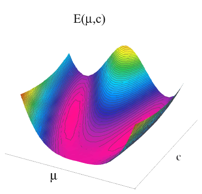
Figure 2: Effective potential as a function o f $c$, one global minimum.

7 Large n

For larger values of $n$, things change, even for $f\gg 0$. Generically, what happens is that as $n$ grows $c_{\rm min}$ tends to zero, but doesn’t quite get there. Thus, as for the case $n=0$, there are still two degenerate minima corresponding to equal and opposite values of $c_{\rm min}$ and so it is possible to lower the energy by forming the states

$$|\psi_{\rm even}\rangle = e^{icp}\left(\cos(\alpha)\,|n_{\gamma}\rangle+\sin(\alpha)\,|n+1_{\gamma}\rangle\right)$$

$$+ e^{-icp}\left(\cos(\alpha)\,|n_{\gamma}\rangle-\sin(\alpha)\,|n+1_{\gamma}\rangle\right)$$

and

$$|\psi_{\rm odd}\rangle = e^{icp}\left(\cos(\alpha)\,|n_{\gamma}\rangle+\sin(\alpha)\,|n+1_{\gamma}\rangle\right)$$

$$- e^{-icp}\left(\cos(\alpha)\,|n_{\gamma}\rangle-\sin(\alpha)\,|n+1_{\gamma}\rangle\right).$$

The result of such a computation is to show that as $n$ grows the splitting between these states grows. Eventually, no matter what value is assigned to $f$ (so long as it is finite) there is a value of $n$ for which the splitting between the states $|\psi_{\rm even}\rangle$ and $|\psi_{\rm odd}\rangle$ becomes of order unity. This is the point at which it makes no sense to talk about tunneling between states defined on one or the other side of the potential barrier.

8 Applying It To Field Theory

For the purpose of this talk I will limit my discussion to the case of $\phi^{4}$-field theory whose Hamiltonian is

$$H\hskip-10.0pt = \hskip-10.0pt\int d^{n}x\left[\frac{1}{2}\Pi_{\phi}(x)^{2}+\frac{1}{2}\left(\nabla\phi(x)\right)^{2}+\frac{\lambda}{6}\phi(x)^{4}\right].$$

It is customary to rewrite the operators $\phi(x)$ and $\Pi_{\phi}(x)$ in terms of their Fourier transforms; i.e.

$$\phi(\vec{k}) = \frac{1}{\sqrt{V}}\int d^{n}xe^{-i\vec{k}\cdot\vec{x}}\phi(x),$$

$$\Pi_{\phi}(\vec{k}) = \frac{1}{\sqrt{V}}\int d^{n}xe^{-i\vec{k}\cdot\vec{x}}\Pi_{\phi}(x),$$ (27)

where $V$ stands for the volume of the system. (I have assumed the system is in a finite volume so that the momenta become discrete and the operators become well defined.)

This Hamiltonian can be rewritten in terms of these momentum space operators as

$$H=\sum_{\vec{k}} \hskip-24.0pt\left[\frac{\Pi_{\phi}(-\vec{k})\Pi_{\phi}(\vec{k})}{2}+\frac{({\vec{k}}^{2}+m^{2})}{2}\,\phi(\vec{k})\,\phi(-\vec{k})\right]$$

$$+\frac{\lambda}{6} \hskip-18.0pt\frac{1}{V}\sum_{\vec{k}_{i}}\phi(\vec{k}_{1})\,\phi(\vec{k}_{2})\phi(\vec{k}_{3})\,\phi(\vec{k}_{4})\delta(\sum_{i=1}^{4}\vec{k}_{i}).$$

To define the adaptive perturbation theory calculation I introduce $\gamma(k)$-dependent annihilation and creations operators as follows,

$$\phi(\vec{k}) = i\,\sqrt{\frac{\gamma(\vec{k})}{2}}({\cal A}(-\vec{k})^{{\dagger}}-{\cal A}(\vec{k}))$$

$$\Pi(\vec{k}) = \frac{({\cal A}(-\vec{k})^{{\dagger}}+{\cal A}(\vec{k}))}{\sqrt{2\,\gamma(\vec{k})}},$$ (29)

The vacuum state associated with this choice of $\gamma(\vec{k})$’s,

$$|vac\rangle=\prod_{k}|0_{\gamma(k)}\rangle,$$ (30)

is defined by the condition that it be annihilated by all the ${\cal A}(\vec{k})$’s.

As in the simpler example I determine the $\gamma(k)$’s by minimizing the vacuum expectation value of the Hamiltonian in this trial state. It follows directly from these definitions that the function to be minimized is

$$\langle vac|\,H\,|vac\rangle\hskip-10.0pt = \hskip-10.0pt\sum_{k}\left[\frac{\gamma(\vec{k})}{4}+\frac{(\vec{k}\cdot\vec{k}+m^{2})}{4\,\gamma(\vec{k})}\right]$$

$$+\frac{\lambda}{4V} \hskip-18.0pt\left[\sum_{\vec{k}}\frac{1}{\gamma(\vec{k})}\right]^{2}.$$ (31)

Obviously, if the range of the momenta appearing in these sums is unrestricted, these expressions diverge. It is customary to deal with this problem, in the context of ordinary perturbation theory, by regulating the integrals and adding counterterms to the Lagrangian to cancel divergences. Since I wish to discuss this theory non-perturbatively, I will adopt a different strategy. I will render the theory well defined by restricting the operators $\phi(\vec{k})$ and $\Pi_{\phi}(\vec{k})$ to be finite in number. This can be accomplished in a variety of ways, but all amount to restricting the range of $\vec{k}$’s which appear in the Fourier transform.

Minimizing Eq. 31 with respect to each $\gamma(\vec{k})$ yields

$$\gamma(k)^{2}=\vec{k}\cdot\vec{k}+m^{2}+2\,\lambda\,\left[\frac{1}{V}\sum_{\vec{k}^{\prime}}\frac{1}{\gamma(\vec{k}^{\prime})}\right].$$ (32)

In particular, the equation for $\vec{k}=0$ is

$$\gamma(0)^{2}=m^{2}+2\,\lambda\,\left[\frac{1}{V}\sum_{\vec{k}^{\prime}}\frac{1}{\gamma(\vec{k}^{\prime})}\right],$$ (33)

which can be substituted into Eq. 32 to give

$$\gamma(\vec{k})^{2}=\vec{k}\cdot\vec{k}+\gamma(0)^{2}.$$ (34)

If we use this to rewrite the equation for $\gamma(0)$, it becomes the non-perturbative equation

$$\gamma(0)^{2}=m^{2}+2\,\lambda\,\frac{1}{V}\sum_{\vec{k}^{\prime}}\frac{1}{\sqrt{(\vec{k}^{\prime})^{2}+\gamma(0)^{2}}}.$$ (35)

Taking $V$ to infinity and converting the sum over $\vec{k}$ to an integral, we obtain an equation which is reminiscent of the Nambu Jona-Lasinio equation.

$$\gamma(0)^{2}-m^{2}\hskip-7.0pt = \hskip-7.0pt\frac{(2\lambda)2^{p}}{(2\pi)^{p}}\int_{0}^{\Lambda}k^{p-1}dk\frac{1}{\sqrt{\vec{k}\cdot\vec{k}+\gamma(0)^{2}}}.$$

In fact Eq. LABEL:NJL should not be thought of as an equation for $\gamma(0)$, but rather as an equation for $m^{2}$; i.e., it should be rewritten as

$$m^{2}=\gamma(0)^{2} \hskip-20.0pt-\frac{(2\lambda)2^{p}}{(2\pi)^{p}}\int_{0}^{\Lambda}k^{p-1}dk\frac{1}{\sqrt{\vec{k}\cdot\vec{k}+\gamma(0)^{2}}}.$$

This shows that for any arbitrarily chosen value of $\gamma(0)$, this equation determines the value of $m^{2}$ for which the chosen value of $\gamma(0)$ will minimize the ground state energy density. This is, of course, nothing but a non-perturbative way of determining the leading mass renormalization counter term.

9 Wavefunction Renormalization

To this point I have shown how a simple variational calculation captures the general notion of mass renormalization in a non-perturbative manner. I now wish to briefly describe what one has to do to capture wavefunction and coupling constant renormalization. The trick is to proceed as in the double well problem and generalize the trial state to include the effects of the ${{\cal A}^{{\dagger}}}^{4}$ and ${\cal A}^{4}$ terms which appear in the normal ordered Hamiltonian; i.e. terms of the form

$$\sum_{k_{1},k_{2},k_{3}} \hskip-20.0pt\frac{1}{4\,\sqrt{\gamma(k1)\,\gamma(k_{2})\,\gamma(k_{3})\,\gamma(k_{4})}}\times$$

$$\left[{\cal A}^{{\dagger}}_{k_{1}}\,{\cal A}^{{\dagger}}_{k_{2}}\,{\cal A}^{{\dagger}}_{k_{3}}\,{\cal A}^{{\dagger}}_{k_{4}}+{\cal A}_{k_{1}}\,{\cal A}_{k_{2}}\,{\cal A}_{k_{3}}\,{\cal A}_{k_{4}}\right]$$

To allow these terms contribute to the ground state energy I have to add to the vacuum state a general four particle state; i.e., I need a trial state of the general form

$$|vac\rangle+\sum\alpha(k_{1},k_{2},k_{3})|4-particle\rangle,$$ (39)

where the sum is assumed to go over all possible four-particle states. The question is ”How do we minimize over the $\alpha(k_{1},k_{2},k_{3})$’s?”.

Actually this question can be finessed since it is equivalent to finding the ground state energy density of a system where the Hamiltonian is truncated to the vacuum state and all possible four particle states. While it is hard to do this for the full Hamiltonian, it can be done for the case where the full Hamiltonian is limited to the part indicated in Eq. LABEL:justfour. In this case the general solution, which will resum the important non-perturbative effects in $\lambda$, can be obtained by considering the resolvent operator. Dividing $H$ into the part diagonal in the number operator and the terms in Eq. LABEL:justfour; i.e.,

$$H=H_{0}+\lambda\,V,$$ (40)

it is easy to show that the resolvent operator satisfies the integral equation

$$\frac{1}{H-z}=\frac{1}{H_{0}-z}-\frac{\lambda}{H_{0}-z}V\frac{1}{H-z}.$$ (41)

This equation is customarily solved by iteration to give the following series;

$$\frac{1}{H-z}=\frac{1}{H_{0}-z} \hskip-20.0pt-\frac{\lambda}{H_{0}-z}V\frac{1}{H_{0}-z}$$

$$+\frac{\lambda^{2}}{H_{0}-z}V\frac{1}{H_{0}-z} \hskip-20.0ptV\frac{1}{H_{0}-z}$$

$$-\frac{\lambda^{3}}{H_{0}-z}V\frac{1}{H_{0}-z} \hskip-20.0ptV\frac{1}{H_{0}-z}V\frac{1}{H_{0}-z}$$

$$+\frac{\lambda^{4}}{H_{0}-z}V\frac{1}{H_{0}-z} \hskip-20.0ptV\frac{1}{H_{0}-z}V\frac{1}{H_{0}-z}V\frac{1}{H_{0}-z}$$

$$+\ldots\ldots\phantom{\frac{\lambda^{4}}{H_{0}-z}\,V}$$ (42)

Since $V$ only links the vacuum to the four particle states and then links four particle states back to the vacuum, this series simplifies to

$$\langle 0|\frac{1}{H-z}|0\rangle = \frac{1}{E_{0}-z}$$

$$+\frac{1}{E_{0}-z}\hskip-10.0pt \hskip-18.0pt\left[\lambda^{2}\sum_{n}\frac{\langle 0|V|n\rangle\langle n|V|0\rangle}{(E_{n}-z)(E_{0}-z)}\right]$$

$$+\left(\frac{1}{E_{0}-z}\right.\hskip-10.0pt \hskip-18.0pt\left.\left[\lambda^{2}\sum_{n}\frac{\langle 0|V|n\rangle\langle n|V|0\rangle}{(E_{n}-z)(E_{0}-z)}\right]\right)^{2}+\ldots$$

$$=\frac{1}{E_{0}-z}\hskip-10.0pt \hskip-18.0pt\left(\sum_{j=0}^{\infty}\left[\lambda^{2}\sum_{n}\frac{\langle 0|V|n\rangle\langle n|V|0\rangle}{(E_{n}-z)(E_{0}-z)}\right]\right)^{j}$$

$$=\phantom{\left(\frac{1}{E_{0}-z}\right.}\hskip-20.0pt \hskip-34.0pt\frac{1}{E_{0}-z-\lambda^{2}\sum_{n}\frac{\langle 0|V|n\rangle\langle n|V|0\rangle}{E_{n}-z}}.$$

Clearly, since the poles of the resolvent operator correspond to the eigenvalues of the Hamiltonian it is only necessary to find that zero of the function

$$E_{0}-z-\lambda^{2}\sum_{n}\frac{\langle 0|V|n\rangle\langle n|V|0\rangle}{E_{n}-z}=0$$ (44)

which lies to the value $E_{0}$ in the limit $\lambda\rightarrow 0$. While this looks like a difficult problem it can be solved to arbitrary accuracy by converting the problem into an equation which can be solved iteratively. To show this I will begin by defining $\delta z$ as

$$z=E_{0}-\lambda\sqrt{\sum_{n}|V|_{0n}^{2}}\ \delta z,$$ (45)

and then use this definition to rewrite Eq. 44 as an integral equation for $\delta z$; i.e.,

$$\delta z=\sum_{n}\frac{|\bar{V}|_{0n}^{2}}{\frac{E_{n}-E_{0}}{\lambda}+\delta z},$$ (46)

where I have defined $\bar{V}_{0n}$ to be

$$\bar{V}_{0n}=\frac{|\langle 0|V|n\rangle|}{\sqrt{\sum_{j}|V|_{0j}^{2}}}.$$ (47)

It is clear that with these definitions, so long as the range of $E_{n}-E_{0}$ is bounded, in the limit $\lambda\rightarrow\infty$ the solution to the integral equation is $\delta z=1$. In other words, in the limit of large $\lambda$ the energy shift is proportional to $\lambda$ instead of the perturbative behaviour which goes like $\lambda^{2}$.

Given the large $\lambda$ value of $\delta z$ it is possible to give an iteration procedure for solving for $\delta z$ for arbitrary values of $\lambda$. This is done by defining a sequence of values $z_{j}$ by the recursion relation

$$\delta z_{0} = 1$$

$$\delta z_{1} = \sum_{n}\frac{|\bar{V}|_{0n}^{2}}{\frac{E_{n}-E_{0}}{\lambda}+\delta z_{0}}$$

$$\delta z_{n} = \sum_{n}\frac{|\bar{V}|_{0n}^{2}}{\frac{E_{n}-E_{0}}{\lambda}+\delta z_{n-1}},$$ (48)

The desired value of $\delta z$ is obtained by taking the limit $n\rightarrow\infty$. As an example, consider the case in which $H$ is a $2\times 2$ matrix with two arbitrary entries on the diagonal $E_{0}$ and $E_{1}$; i.e.,

$$H=\left(\begin{array}[]{*{2}{c@{\quad}}}E_{0}&x\\ &\\ x&E_{1}\\ \end{array}\right).$$

Since it is trivial to diagonalize this matrix it is easy to compare, for the case $E_{0}=1$ and $E_{1}=2$, the iterative solution for arbitrary $x$ to the exact answer. Figure 3 shows how a single iteration manages to reproduce the behavior of the exact answer to pretty good accuracy over the whole range of $x$.

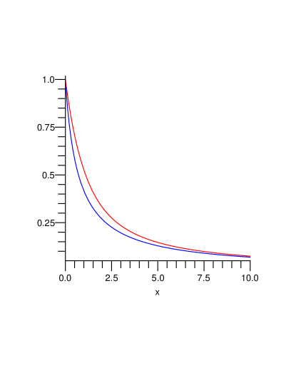
Figure 3: Comparison of exact energy as a function of $x$ (red curve) compared to $\delta z_{1}$ (blue curve)

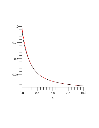
Figure 4: Comparison of exact energy as a function of $x$ (red curve) compared to $\delta z_{3}$ (blue curve)

After three iterations it is much harder to distinguish the curves, see Fig. 4. Doing more iterations just produces better and better accuracy over the entire range. By twelve iterations one is accurate to very high accuracy except in a very small band around $x\approx 0.8$, where the fractional error is $\approx 0.015$. The same computation can be done for the more realistic case where $V$ connects us to a large number of momenta, with similar results.

Having established that it is in principle possible to obtain the shift in the ground state energy due to the part of the Hamiltonian which mixes the vacuum with four particle states, it is time to go back to our discussion of the adaptive perturbation theory scheme. Given the preceding discussion it is easy to show that differentiating the expectation value of the Hamiltonian in our trial state will yield a set of equations for the $\gamma(k)$’s of the general form

$$\frac{1}{4}-\frac{(k^{2}+m^{2})}{4\,\gamma(k)^{2}}\hskip-20.0pt -\frac{\lambda}{2\gamma(k)^{2}}\left[\frac{1}{V}\sum_{k^{\prime}}\frac{1}{\gamma(k^{\prime})}\right]$$

$$-\frac{\lambda^{2}}{\gamma(k)^{2}}\hskip-10.0pt \hskip-10.0pt\,\Sigma(k^{2},\lambda,\gamma(k_{i}))=0,$$ (49)

where the function $\Sigma(k^{2},\lambda,\gamma(k_{i}))$ is obtained by differentiating the solution for $\delta z$ obtained from our integral equation. In writing things in this form I used the fact, which can be obtained from the integral equation, that differentiating $\delta z$ with respect to a given $\gamma(k)$ produces a factor of $\gamma(k)^{-2}$ multiplied by a function of $k^{2}$,$\lambda$ and all the $\gamma(k_{i})$. As in the earlier discussion of mass renormalization, it is convenient to rewrite these equations as

$$\gamma(k)^{2}=k^{2}+m^{2} + 2\,\lambda\,\left[\frac{1}{V}\sum_{k^{\prime}}\frac{1}{\gamma(k^{\prime})}\right]$$ (50)

$$+ \lambda^{2}\,\Sigma(k^{2},\lambda,\gamma(k_{i}))$$

and then observe that this means that

$$\gamma(0)^{2}=m^{2} + 2\,\lambda\,\left[\frac{1}{V}\sum_{k}\frac{1}{\gamma(k)}\right]$$ (51)

$$+ \lambda^{2}\Sigma(0,\lambda,\gamma(k_{i})).$$

Substituting this into the equation for a generic value of $k$ yields

$$\gamma(k)^{2} = k^{2}+\gamma(0)^{2}$$

$$+ \lambda^{2}\left(\Sigma(k^{2},\lambda,\gamma(k_{i}))-\Sigma(0,\lambda,\gamma(k_{i}))\right).$$

At this point the role of wavefunction renormalization becomes obvious. If, as is conventional, we Taylor series expand $\Sigma(k^{2},\lambda,\gamma(k_{i}))$ so as to rewrite Eq. LABEL:wvrenone as

$$\gamma(k)^{2} = (1+\frac{\partial}{\partial k^{2}}\Sigma(k^{2}),\lambda,\gamma(k_{i}))k^{2}+\gamma(0)^{2}$$ (53)

$$+ \lambda^{2}\left(\Sigma(k^{2},\lambda,\gamma(k_{i}))-\Sigma(0,\lambda,\gamma(k_{i}))\right.$$

$$- \left.k^{2}\frac{\partial}{\partial k^{2}}\Sigma(0,\lambda,\gamma(k_{i}))\right).$$

This can be put into a conventional form

$$\gamma(k)^{2}=k^{2}+\gamma(0)^{2}+\lambda^{2}\bar{\Sigma}(k^{2},\lambda,\gamma(k_{i}))$$ (54)

by introducing a rescaling of the fields and the overall Hamiltonian by

$$\phi \rightarrow Z_{\phi}^{1/2}\phi\quad;\quad\Pi_{\phi}\rightarrow\frac{\Pi_{\phi}}{Z_{\phi}^{1/2}}$$

$$H \rightarrow Z_{\phi}H.$$ (55)

Thus, we see that wavefunction renormalization is just that, an overall change in the $\gamma(k)$’s. Note that the rescaling of the Hamiltonian is necessary because we are working in a Hamiltonian and not a manifestly covariant formalism.

Finally, I will just say a few words about coupling constant renormalization and why $\phi^{4}$ theory doesn’t exist in four dimenstions, at least if one attempts to remove the cutoff. Clearly, once the $\gamma(k)$’s have been chosen, the only remaining issue is determining those values of $\lambda$ for which some physical quantity come out finite. For the purposes of this discussion I can choose this to be the energy of a trial state containing only two particles of momentum zero.

As in earlier discussions I will restrict this analysis to the effect of terms in $H$ which take two particles to two particles. In this case I can employ a similar argument, based upon studying the matrix element of the resolvent operator in this zero-momentum state, to show that in four dimensions this energy is given by a series in $\lambda\left(\lambda\ln(\Lambda)\right)^{n}$. From this it follows that the only way to have this come out finite is to take $\lambda\rightarrow 1/\ln(\Lambda)$. But this, of course, implies that there is no interaction.

10 The Spectrum Isn’t Boost Invariant

The final point which should be touched upon before closing my talk is the observation that at first glance an equation of the form

$$\gamma(k)^{2}=k^{2}+\gamma(0)^{2}+\lambda^{2}\bar{\Sigma}(k^{2},\lambda,\gamma(k_{i}))$$ (56)

would seem to be problematic, since $\gamma(k)$ for $k\neq 0$ is not just related by a boost to the value for $k=0$. In fact, this is not a bug, it is a feature. What it says is that while it is possible to choose the $\gamma(k)$’s to give a good perturbation perturbation theory, with this choice of $\gamma(k)$’s the operators ${\cal A}^{{\dagger}}(k)$ do not create a true asymptotic states which should be used to compute scattering amplitudes. Even if I assume that the state created by ${\cal A}^{{\dagger}}(0)$ is a good approximation to the zero momentum state, the state for $k\neq 0$ should be obtained by applying the boost operator to this state. For an interacting theory this is certainly a multi-particle state. Thus, it follows that adopting the formalism of adaptive perturbation theory forces implies that the scattering problem must be handled as in the parton picture. In other words, the computation of a scattering process intrinsically has two parts; first, it is necessary to find the parton wavefunction for the asymptotic scattering states and then, this wavefunction, together with the explicit form of the Hamiltonian written in terms of the annihilation and creation operators associated with the specific choice of $\gamma(k)$’s, should be used to compute scattering amplitudes. This point, together with the observation that applying a boost (written in terms of the relevant annhilation and creation operators) to a given state implies a kind of Alterelli-Parisi equation, requires much more thought.

11 Summary

In this talk I began by showing you how to convert problems, which in the past were thought to be impossible to deal with perturbatively, can be easily done using the method I have called adaptive perturbation theory. I then went on to show how these methods can be extended to give a very pretty picture of the structure of renormalization in a non-perturbative context. These ideas can be extended to a theory which includes fermions by adding adding a general Bogoliubov transformation for the fermion fields defined in momentum space. A bit more work has to be done to extend the tricks to cover the case of compact Abelian gauge-fields. However, a paper by David Horn and myself[7], extended in the obvious way to fit it into the framework of adaptive perturbation theory, showed how to do this for the case of compact QED. This paper showed that the method is quite capable of extracting the interesting non-perturbative structure of confinement in this theory in any number of space-time dimensions. While the path towards extending these ideas to the case of a non-abelian gauge theory is not so obvious, I nevertheless believe that it is possible.

References

- [1] Subsequent to completing this work I was made aware of previous papers by I. D. Feranchuk and collaborators, who, in a series of very interesting papers, developed a method whose basic idea is the same as the approach described in this paper. These authors then applied this method to a wide variety of problems in quantum mechanics, demonstrating the rapid convergence of the approximation scheme. Although our way of implementing the basic idea differs in significant ways, the fundamental ideas are the same and so, the applications these authors discuss can also be treated by the methods I describe. The introduction of their approach and some of the applications they treat in beautiful detail can be found in the following papers: I. D. Feranchuk and L. I. Komarov J. Phys. C 15 (212)1965, I. D. Feranchuk and L. I. Komarov Phys. Lett. A 88 (212)1982, I. D. Feranchuk and L. I. Komarov J. Phys. A 17 (3111) 1984, Le Anh Thu and L. I. Komarov arxiv cond-mat/9812323 (ref therein), I. D. Feranchuk and A. L. Tolstik J. Phys. A 32 (2115) 1999, Feranchuk arxiv cond-mat/0510510
- [2] I. G. Halliday and P. Suranyi, Phys. Lett. B 85, 421 (1979).
- [3] I. G. Halliday and P. Suranyi, Phys. Rev. D 21, 1529 (1980).
- [4] V. F. Weisskopf and E. P. Wigner, Z. Phys. 63, 54 (1930); 65, 18 (1930).
- [5] B. Simon and R. Griffiths,Comm. Math, Phys.,bf 33, 145, (1973)
- [6] This sort of variational computation for the case of field theory has a colorful history. The application of the simplest version of these ideas to negative mass field theory was, to the best of my knowledge first done by Arthur Wightman and a student. I was made aware of this in a private discussion with Sidney Coleman sometime before 1970. This discussion was precipitated by the fact that Sidney Drell and I had rediscovered this computation sometime before 1974 and were very taken with the simplicity of the approach. Unfortunately, for exactly the same reason as in my discussion of the double well, this computation predicted a first order phase transition at a non-vanishing value of external field and Coleman pointed out to us that, in the case of dimensions, this violated a theorem by Simon and Griffiths[5]. At the time we didn’t really understand the origin of this problem. Subsequently the same calculation was published by S. J. Chang Phys. Rev. D 12 (1071)1975, where he too pointed out that the result violated an exact theory in the case of dimensions. Chang’s paper was followed by a paper by Paolo Cea and Luigi Tedesco Phys. Rev. D 55 (4967), which presented a field theory improvement of S. J. Chang’s computation based upon a diagrammatic perturbation theory which eliminated by false tri-critical behavior, but not at the level of the variational computation. Subsequently a systematic perturbation theory about the variational calculation was discussed by Jeff Rabin Nuclear Physics B 224 (308-328) 1983. So far as I know, no variational way of removing the tri-critical behavior was published before the analysis in this paper.
- [7] D. Horn and M. Weinstein, Phys. Rev. D 25, 3331 (1982).