Strings on AdS₃$\times$S³ and the Plane-Wave Limit

Issues on PP-Wave/CFT Holography

Advisor:
Prof. Massimo Bianchi (Univ. Tor Vergata)

Evaluating Commmittee:
Prof. Ignatios Antoniadis (CERN)
Prof. Edi Gava (ICTP)

Rome, March 2005

$\star$

A mis seres más queridos:
Lili, mi papá, mi mamá,
Emiliano, Paco y Serenita

Acknowledgements

I am grateful to Massimo Bianchi for his assistance and friendship during my studies. I am also indebted to F. Fucito, G. Pradisi, Ya. Stanev and, specially, A. Sagnotti, for patiently teaching me theoretical physics.

I enjoyed many discussions with my collaborators: M. Bianchi, G. D’Appollonio, E. Kiritsis and K. L. Panigrahi.

I would like to recognize and thank the Istituto Nazionale di Fisica Nucleare and the ICSC World-Laboratory, in particular its President Prof. A. Zichichi, for financial support during part of my PhD. My thanks to the Abdus Salam International Center for Theoretical Physics in Trieste, where I enjoyed a peaceful time to write this thesis. I am also grateful to the Max Planck Institute for Gravitational Physics in Berlin, and its director H. Nicolai, for hospitality during completion of this work.

I am deeply acknowledged to all the people who made possible, and sometimes impossible, my stay in Rome. Special thanks to Alfredo, Bruno, Fabrice, Jovanka, Kamal, Lea, Marco, Maurizio, Paco and Vladimir.

A big thank you to all the graduate students of the group.

Dejo aquí constancia de la deuda contraída con mi amigo y mentor Cmdte. Luigi: ‘gracias por haberme contagiado parte de tu entusiasmo por la física teórica’.

Chapter 1 Introduction and Conclusions

It is strongly believed that the Standard Model of particle physics is just an excellent low energy limit of a more fundamental theory that must account for physics at very high energies. For more than twenty years the SM has successfully described data from experiments probing energies up to the order of 1 TeV. It has also predicted new particles and phenomena subsequently verified, and it continues to provide new insights into our physical world. In spite of this, at higher energies new physics could appear and new theoretical frameworks should explain it. A viable framework to deal with is String Theory, a theory that assumes that the fundamental building blocks of nature are one-dimensional objects, i.e., strings.

String Theory is a quantized theory of gravity that is expected to be also a unified model of all the fundamental interactions. More recently there has been a renewal of interest in understanding the link between string theory and particle physics, this in order to find an exact description of confining gauge theories in terms of strings. The idea is not new and goes back to the early ’70 when ’t Hooft proposed a dual model of strings for describing gauge theories with a large number of colors.

In order to clarify this duality it is convenient to introduce the concept of Black Hole, a very massive object originated in a gravitational collapse, inside of which all the forces of nature are in action. For our purposes, a Black Hole (BH) simply can be regarded as a region of spacetime from where no information can escape beyond its boundary, i.e., the information inside the BH is inaccessible to distant observers. Moreover, Black Holes are very simple objects since their properties do not depend on the kinds of constituents they are made of, but instead in some basic properties as the mass, charge and angular momentum.

The simplest black hole, the Schwarzschild BH, has a Event Horizon which is a sphere of area $A=4\pi G^{2}M^{2}/c^{4}$. It can be proved that this area cannot decrease in any classical process. On the other hand, gravitational collapsing objects which give rise to black holes seem to violate the second law of thermodynamics. This is easy to see: since the initial collapsing object has a non-vanishing entropy and the final BH cannot radiate, hence, the entropy of the system has decreased. The problem is solved by providing an entropy to the Black Hole. For a Schwarzschild BH it was proposed by Bekenstein that the entropy is proportional to the Event Horizon area, a quantity that can only increase as the entropy does in classical thermodynamics,

$$S_{BH}=\frac{1}{4}\frac{A}{l_{p}^{2}}~{}.$$ (1.1)

The Generalized Second Law (GSL) of thermodynamics extends the usual Second Law to include the entropy of black holes in a composite system, counting the entropy of the standard matter system and also that of the black hole: $S_{TOT}=S_{MATT}+S_{RAD}+S_{BH}$. This is the entropy that always increases. Starting with a collapsing object of entropy $S$, the GSL of thermodynamics imposes that $S\leq S_{BH}$. This is the Holographic Bound, and it states that the entropy of a matter system entirely contained inside a surface of area $A$, cannot exceed that of a black hole of the same size. Alternatively, the Holographic Bound can be rephrase saying that the information of a system is completely stocked in its boundary surface.

This statement is generalized by the Holographic Principle. It claims that any physical process occurring in $D+1$ spacetime dimensions, as described by a quantum theory of gravity, can be equivalently described by another theory, without gravity, defined on its $D$-dimensional boundary. Some authors believe that this statement is universal and a fundamental principle of nature. Nevertheless, the principle has been tested only in few cases. An example is the AdS/CFT correspondence, that exactly relates superstring theory in a $D$-dimensional space with a superconformal field theory on the boundary.

Finally, we would like to comment on the Black Hole Information Paradox and see how the Holographic Principle resolves it. The paradox can be posed in the following terms. Since a collapsing object is in a definite quantum state before it starts to contract, we expect the final object to be in exactly the same configuration. However, the thermal radiation of the BH comes as mixed states and so the information we get from the inside of the BH does not reproduce the information booked in the original object. We can say that the initial information is lost inside the Black Hole. This paradox is solved by the Holographic Principle, since the full dynamics of the gravitational theory is now described by a standard, though complex, quantum system with unitary evolution.

So far the most accurate holographic proposal relating gauge theories to strings is the novel AdS/CFT correspondence. In two words, it says that ST defined in a negatively curved anti-de Sitter space (AdS) is equivalent to a certain Conformal Field Theory (CFT) living on its boundary. One concrete example is AdS₅/CFT₄: it states that type IIB superstring theory in AdS₅ is equivalently described by an extended ${\cal N}=4$ super-CFT in four dimensions. The other five dimensions of the bulk are compactified on S⁵. The five-sphere with isometry group $SO(6)$ is chosen in order to match with the $SU(4)$ R-symmetry of the super Yang-Mills theory. The AdS/CFT correspondence is a weak/strong coupling duality, allowing us to probe the strong coupling regime in the gauge theory from perturbative means in the string side, and viceversa. This can be seen from the fundamental relation between the superstring side of the correspondence and the super-Yang-Mills theory

$$\left(\frac{R}{l_{s}}\right)^{4}=4\pi g_{s}N~{}\leftrightarrow~{}g_{YM}^{2}N\equiv\lambda~{},$$ (1.2)

where $R$ is the curvature radius of the anti-de Sitter space, $N$ is the number of colors (considered very large) in the gauge group and $\lambda$ is the ’t Hooft coupling.

In the Supergravity limit the string length is much smaller than the radius of the AdS space, given

$$1\ll\left(\frac{R}{l_{s}}\right)^{4}~{}\leftrightarrow~{}\lambda~{}.$$ (1.3)

In this limit the bulk theory is manageable, being ${\mathcal{N}}=8$ Gauged Supergravity, but in the boundary side it turns out that the gauge theory is in a strongly couple regime, where a perturbative analysis is senseless. This establishes the weak/strong coupling nature of the duality. This is an advantage is we want to study the strongly coupled regime of one of the theories, since we can always use perturbative results in the dual theory. However, the difficulties in finding a common perturbative sector where to test the correspondence makes it very hard to prove its full validity. The strong formulation of the AdS/CFT correspondence claims its validity at the string quantum level, nevertheless, so far no one has been able to quantitatively prove it beyond the classical Supergravity approximation.

The main challenges of AdS/CFT are two-fold: i)  to shed light in the strongly regime of non-abelian theories, as a step further in the understanding of more realistic QCD-like theories; ii) to provide a full proof of the correspondence. The latter is a non-trivial task since we do not have an independent non-perturbative definition of string theory in order to compare it with the boundary theory in the strongly coupled regime. Pointing in this direction, a couple of years ago a new proposal was suggested, that goes under the name of BMN Conjecture, and opened the possibility to test the correspondence beyond the SUGRA limit.

Since the two-dimensional sigma model for superstrings on AdS₅$\times$S⁵ supported by R-R flux is far from been manageable, even at the non-interacting level $g_{s}=0$, the proof of the stringy regime of the AdS/CFT correspondence is hard to carry off. Nevertheless, under some conditions, it was found by Berenstein, Maldacena and Nastase (BMN) that the two sides of the correspondence have an overlapping perturbative regime that allows for a test of the duality at the stringy regime.

Long before the AdS/CFT duality, it was known that type IIB superstring theory had two maximally supersymmetric spaces: flat ten-dimensional spacetime and AdS₅$\times$S⁵. More recently it was discovered that in the Penrose limit AdS₅$\times$S⁵ reduces to a gravitational plane-wave, PP-Wave for short, that gives the third and last maximally supersymmetric space of type IIB superstring. In this background the theory was shown to be described by a free, massive, two-dimensional worldsheet sigma model easily quantizable in the light-cone gauge. With these exact string results at hand, it remained to associate the limit in the bulk to a process in the boundary theory. This last step was fulfilled by BMN.

In the bulk, the energy of a state is given by the generator of translations in time $E=i\,\partial_{t}$, and the angular momentum around a great circle of S⁵ is associated to $J=-i\,\partial_{\phi}$. The light-cone hamiltonian and momentum can be taken to be

$$H_{lc}\equiv\,\partial_{x^{+}}\propto E-J~{},\qquad P_{lc}\equiv\,\partial_{x^{-}}\propto\frac{E+J}{R^{2}}~{},$$ (1.4)

where $x^{\pm}$ are the spacetime light-cone coordinates, and an explicit formula for $H_{lc}$ is known. From the second equation, we note that the condition of non-vanishing light-cone momenta selects those angular momenta going with the radius $R$ as $J\propto R^{2}$. Moreover, the limit $N\to\infty$ imposes $J^{2}\sim N$. It turns out that this limit is different from the large $N$ limit we comment above since in that case the expansion in $\lambda\equiv g_{s}N$ implied $g_{s}$ small, something not required by the present approach.

On the other side of the correspondence, the energy $E$ is identified with the scaling dimension $\Delta$ of the operator on the boundary. The angular momentum $J$ is associated to an $U(1)$ subgroup of the $SU(4)$ R-symmetry of ${\cal N}=4$ super Yang-Mills. With these identifications, the fundamental relation of the BMN correspondence is settled to be

$$H_{lc}\propto\Delta-J~{}.$$ (1.5)

As we said before, according to the AdS/CFT duality the limit we carry out in the bulk should have certain consequences in the boundary. BMN conjecture states that the limit has its counterpart in a truncation of the class of operators defined in the superconformal theory. Only operators with large R-charge and $\Delta\sim J$ survive the limit, including string excitations.

The BMN conjecture opens the possibility to test the AdS/CFT correspondence beyond the supergravity regime, nevertheless, not all the ideas involved are conceptually well established. One of these is the fate of holography in the BMN limit. It seems that the beautiful holographic picture of the AdS/CFT duality is completely lost in the plane-wave background. But maybe a remnant of it can survive.

This Thesis

The main obstacle towards a complete understanding of the holographic duality beyond the supergravity approximation, that captures the strongly coupled regime of the boundary conformal field theory, is our limited comprehension of the quantization of superstring theory in R-R backgrounds. One possible exception is the background AdS₃$\times$S³$\times$$\mathcal{M}$ supported by a NS-NS three-form flux, which is the near horizon geometry of a bound-state of fundamental strings (F1) and five-branes (NS5). Since the dynamics on the world-sheet is governed by an $\widehat{SL}(2,{\mathbb{R}})\times\widehat{SU}(2)$ Wess-Zumino-Witten model, string amplitudes can be computed using CFT techniques. The dual two-dimensional superconformal field theory is expected to be the non-linear sigma model with target space the symmetric orbifold ${\mathcal{M}}^{N}/{\mathcal{S}}_{N}$, where $\mathcal{M}$ can be either T⁴ or $K3$.

In this thesis we give explicit results for bosonic string amplitudes on AdS₃$\times$S³ and the corresponding plane-wave limit. We also analyze the consequences of our approach for understanding holography in this set up, as well as its possible generalization to other models. The original materials appeared (or are to appear) in a series of publications by the author and collaborators [1, 2, 3, 4].

• Chapter 2: After reviewing the physics of the two sides of the AdS₃/CFT₂ correspondence, we perform the plane-wave limit in an heuristic way in order to set the basis of the more technical material that follows in this thesis. In general, a precise correspondence between bulk and boundary dynamics has been a longstanding challenge in AdS/CFT. A discussion on the AdS₃/CFT₂ discrepancy at the supergravity level can be found in the last part of this chapter.

• Chapter 3: We recall the necessary tools for dealing with Wess-Zumino-Witten (WZW) models and display the full spectrum of strings on AdS₃$\times$S³. We then compute bosonic string amplitudes on this background and determine their Penrose limit. A crucial role is played by the charge variables that, from a group theoretical point of view, are introduced in order to encode the content of the (in) finite dimensional irreducible representations. More physically, they are seen as coordinates in the holographic boundary. In this approach, plane-wave chiral primaries are obtained by rescaling the charge variables with the level of the algebras $k_{1},k_{2}\to\infty$.

• Chapter 4: We compute tree-level bosonic string amplitudes in the Hpp-wave limit of AdS₃$\times$S³ supported by NS-NS three-form flux. The corresponding WZW model is obtained contracting the algebras $\widehat{SL}(2,\mathbb{R})_{k_{1}}$ and $\widehat{SU}(2)_{k_{2}}$ according to $k_{1},k_{2}\to\infty$ with $\mu_{1}^{2}k_{1}=\mu_{2}^{2}k_{2}$. We examine the irreducible representations of the model and define vertex operators. We then compute two, three and four-point functions. As a starting point for more realistic models, we consider only scalar tachyon vertex operators with no excitation in the internal worldsheet CFT. The computation of such string scattering amplitudes heavily relies on current algebra techniques on the worldsheet, generalizing in some sense the results for the Nappi-Witten model developed in [5]. We show that these amplitudes exactly match the ones computed in the third chapter. It is worth stressing that these amplitudes are well defined even for $p=0$ states, which are difficult (if not impossible) to analyze in the light-cone gauge. We have thus provided further evidence for the consistency of the BMN limit in this setting.

• Chapter 5: We propose an extension of the previous procedure and the holographic interpretation of the charge variables to more interesting and realistic models. While for the $\widehat{SL}(2,\mathbb{R})_{L}\times\widehat{SL}(2,\mathbb{R})_{R}$ algebra, underlying AdS₃, the charge variables $x$ and $\bar{x}$ can be viewed as coordinates on the two-dimensional boundary, in the case of the $\widehat{\mathcal{H}}_{2+2n}$ algebra, underlying a pp-wave geometry, the corresponding charge variables $x^{\alpha}$ and $x_{\alpha}$ become coordinates on a $2n$-dimensional holographic screen [6]. This picture replaces the one-dimensional null boundary representing the geometric boundary in the Penrose limit. The approach with charge variables suggests that correlation functions in the BMN limit of ${\mathcal{N}}=4$ super-CFT are indeed well defined and computable.

• Chapter 6: Emphasizing on the holographic charge variables we tackle the full superstring model. We construct vertex operators and give instructions on how to compute scattering amplitudes in the Hpp-wave limit and interpret their structure. In principle, one would like to address important issues as the spectrum, trilinear couplings and operator mixing in a more quantitative way. In the last part we propose a precise correspondence between states in the symmetric product and superstring vertex operators.

• Appendix A: The alternative Wakimoto free field representation is given and string amplitudes computed. These results are shown to coincide with the amplitudes of chapter 3 and 4.

Alternatively, one may consider turning on R-R fluxes. The hybrid formalism of Berkovits, Vafa and Witten [7] seems particularly suited to this purpose as it allows the computation of string amplitudes, at least for the massless modes [8], and the study of the Penrose limit in a covariant way [9]. The mismatch for 3-point functions of chiral primaries (or rather their superpartners) and the consequent lack of a non-renormalization theorem for these couplings calls for additional investigation in this direction and a careful comparison with the boundary CFT results. Once again, the BMN limit may shed some light on this issue as well as on the short-distance logarithmic behavior, found in [10] for AdS₃ and in [5] for NW, that could require a resolution of the operator mixing or a scattering matrix interpretation.

In this thesis we have argued that the BMN limit of physically sensible correlation functions are well defined and perfectly consistent, at least for the CFT dual to AdS₃$\times$S³. In particular it should not lead to any of the difficulties encountered in the case of ${\cal N}=4$ SYM as a result of the use of perturbative schemes or of the light-cone gauge. In conclusion, we hope we have presented enough arguments in order to consider (super) strings on the plane-wave limit of AdS₃$\times$S³ supported by NS-NS fluxes as a source of extremely useful insights in holography and the duality between string theories and field theories.

Chapter 2 Overview of AdS₃/CFT₂

In this chapter we present the state of the holographic correspondence holding between string theory in AdS₃ and the two-dimensional CFT living on its boundary [11]. This chapter is organized as follows. In section 2.1 we first introduce the anti-de Sitter spaces, the geometry relevant for the correspondence, and then we review the microscopic physics of some generalized black holes. In the last part of this section we comment on the core idea of the correspondence, i.e., its holographic property. In section 2.2 we describe the dynamics of strings moving on general group manifolds, in particular on AdS₃. From a semi-classical analysis we get a valuable geometrical picture of the quantum spectrum. In section 2.3 we introduce the AdS₃/CFT₂ correspondence. Finally, in section 2.4 we discuss the possibility of testing the AdS/CFT correspondence beyond the supergravity approximation, in concrete, in the plane-wave limit.

2.1 Anti-de Sitter spaces and black holes

Anti-de Sitter geometries are solutions of Einstein equations of motion with negative cosmological constant $\Lambda$ =$-(D-1)(D-2)/2R^{2}$, where $D$ is the number of spacetime dimensions of the AdS space and $R$ its curvature radius. These spaces have the important property of being maximally symmetric, or in other words, to have a maximal number of Killing vectors, in all $D(D+1)/2$. The AdS_p+2/CFT_p+1 correspondence proposes the identification of the isometry group of AdS_p+2 with the conformal symmetry of the flat Minkowski space ${\mathbb{R}}^{1,p}$.

An AdS_p+2 space of curvature radius $R$ can be defined by the connected hyperboloid [12]

$$X_{-1}^{2}+X_{0}^{2}-\sum_{i=1}^{p+1}X_{i}^{2}=R^{2}~{},$$ (2.1)

where $X_{M}$ $(M=-1,0,\dots\,p+1)$ are the coordinates on the embedding space. The latter is a (p+3)-dimensional flat space ${\mathbb{R}}^{2,p+1}$ with metric

$$ds^{2}=-dX_{-1}^{2}-dX_{0}^{2}+\sum_{i=1}^{p+1}dX_{i}^{2}~{}.$$ (2.2)

From here we see that the AdS_p+2 space has isometry group SO$(2,p+1)$ and by construction is homogeneous and isotropic. Even if by definition the ambient space has two time directions, notice that one of them is orthogonal to the hypersurface defining the AdS space, leaving us with only one time direction as desired. As we will see below, the closed timelike curves arising in this picture can be avoided by choosing an appropriate set of coordinates (global coordinates, see below) and then unwrapping the time direction.

We can now define global coordinates on the hyperboloid (2.1)

$$X_{-1} = R\cosh\rho\,\sin\tau~{},\qquad X_{0}=R\cosh\rho\,\cos\tau~{},$$

$$X_{i} = R\sinh\rho\,\Omega_{i}~{},$$ (2.3)

with $i=1,\dots,p+1$ and $\sum_{i}\Omega_{i}^{2}=1\,$. Inserting (2.1) in the metric (2.2), this takes the form

$$ds^{2}=R^{2}\,(-\cosh^{2}\rho\,d\tau^{2}+d\rho^{2}+\sinh^{2}\rho\,d\Omega^{2})~{}.$$ (2.4)

It is worth remarking that the global coordinates cover the whole AdS space. We can get rid of closed timelike curves by considering a non-compact coordinate system where time is non-compact, $-\infty<\tau<\infty$. When talking about the AdS/CFT correspondence we will always refer to this covering space.

Another useful parametrization is given by the Poincaré coordinates,

$$X_{-1} = Ru\,t,\qquad\qquad X_{0}=\frac{1}{2u}\,[1+u^{2}(R^{2}+\vec{x}\,^{2}-t^{2})],$$

$$X_{i} = Ru\,x_{i},$$

$$X_{p+1} = \frac{1}{2u}\,[1-u^{2}(R^{2}-\vec{x}\,^{2}+t^{2})],$$ (2.5)

where (this time) $i=1,\dots,p$ . With this change of variables, the induced metric on AdS_p+2 becomes

$$ds^{2}=R^{2}\left[u^{2}(-dt^{2}+d\vec{x}\,^{2})+\frac{du^{2}}{u^{2}}\right].$$ (2.6)

Since in this thesis we will be particularly interested in AdS₃ spaces, ${\it i.e.},$ $p=1$ in our notation, it will be helpful to have the metric in global coordinates for this special case

$$ds^{2}=R^{2}(-\cosh^{2}\rho\,d\tau^{2}+d\rho^{2}+\sinh^{2}\rho\,d\phi^{2}),$$ (2.7)

where the unit vector $\Omega_{i}\,$ in (2.4) reduces to a single parameter $\phi$. In terms of this coordinates and choosing the universal covering range already mentioned, $0\leq\rho<\infty\,$, $-\infty<\tau<\infty$ and $0\leq\phi<2\pi$, the AdS₃ space can be seen as a solid cylinder (see Figure 2.1).

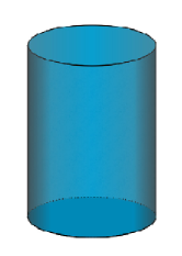
Figure 2.1: Representation of an AdS₃ space in global coordinates.

For later use, let us also write down the full AdS₃$\times$S³ metric in global coordinates

$$ds^{2}=R^{2}(-\cosh^{2}\rho\,d\tau^{2}+d\rho^{2}+\sinh^{2}\rho\,d\phi^{2})+R^{2}(\cos^{2}\theta\,d\psi^{2}+d\theta^{2}+\sin^{2}\theta\,d\varphi^{2}).$$ (2.8)

Both spaces have radius $R$. The variables $0\leq\theta,\psi,\varphi<2\pi$ are angles in the three-sphere.

The boundary of AdS_p+2 is the $p+1$-dimensional surface at $\rho\to\infty$, a region that cannot be reached by a massive particle while a light ray can go and get back in a finite time. The AdS/CFT correspondence states that the dual description of the gravity theory lives precisely in this boundary space. We will come back to this later on. After this overview of Anti-de Sitter spaces now we would like to understand how these backgrounds can be generated from string theory principles and what is their exact role in the correspondence.

In the middle nineties it was shown that there are only five consistent superstring theories (types IIA, IIB, HE and HO with closed strings and type I that unavoidably contains both open strings and closed strings), all of them living in ten spacetime dimensions. This was supported by the idea that some of the theories were related between them by fundamental symmetries, and by the fact, unexpectedly, that non-perturbative dualities of type-II theories allowed for R-R $p$-brane solutions in supergravity – the low energy effective theory of the corresponding superstring. Moreover, $p$-branes were shown to have an equivalent description in terms of hyperplanes in spacetime, a sort of R-R charged membranes – in fact BPS solitons, which in turn can be a source of closed strings. These last objects are called Dp-branes. They are non-rigid hyperplanes with $p$ space dimensions and $p+1$ dimensional world-volume. Due to the open-closed duality of the string models, the $Dp$-branes are also supposed to be the slices of space where the ends of an open string can sit (see [14] for an introduction to string theory). This dual vision of $Dp$-branes is at the heart of the most exciting developments in string theory, including the celebrated AdS/CFT correspondence.

D$p$-branes are solutions of supergravity equations, and it can be proved that for type IIB theory the only admissible BPS D$p$-branes are for $p=-1,\,1,\,3,\,5,\,7,\,9$, each of them been a particular solution. But not all imaginable configurations of branes produces new supergravity solutions, actually a D$p$-D$p^{\prime}$ configuration needs to satisfy some conditions in order to generate a stable solution, compensating the R-R charge repulsion with some attractive potential. For the D1-D5 system we will be concerned with, the condition $p-p^{\prime}=4$ insures that we have a stable configuration, or in other terms a bound state at threshold. By this procedure the supergravity solution we will get at first hand is not the AdS₃$\times$S³ space we are looking for, but instead a more complex space that in a certain limiting region reduces to it. To present our analysis in the more convenient way, we choose to begin generating this more general space and then going to the suitable limiting case.

The relevant set-up for AdS₃$\times$S³ consists in D1-branes living on D5-branes. To visualize it let us draw a table showing where the branes are located.

	$x_{0}$	$x_{1}$	$x_{2}$	$x_{3}$	$x_{4}$	$x_{5}$	$x_{6}$	$x_{7}$	$x_{8}$	$x_{9}$
D1	–	–	$\perp$	$\perp$	$\perp$	$\perp$	$\perp$	$\perp$	$\perp$	$\perp$
D5	–	–	$\perp$	$\perp$	$\perp$	$\perp$	–	–	–	–

Table 1. The D1-D5 brane configuration.

A dash under the coordinate $x_{M}$ ($M=0,\,\dots,\,9$) means that the brane is extended in that direction. On the other hand, a $\perp$ symbol means that the brane is perpendicular to $x_{M}$, or in other words that the brane looks like a point particle along that direction. It can be seen that due to the presence of the D-branes the ten dimensional Lorentz symmetry is broken from the original $SO(1,9)$ to $SO(1,1)_{01}\times SO(4)_{2345}\times SO(4)_{6789}$, where the indices stand for the spacetime directions shown in Table 1. Truly speaking, in string theory the $SO(4)_{6789}$ symmetry is broken by wrapping the directions on the four dimensional manifolds T⁴ (or $K3$), but at low energies the compactified dimensions are too small, restoring it as a symmetry of the supergravity solution, $U(1)^{4}\to SO(4)_{6789}$.

The D1-D5 brane configuration described above is a IIB supergravity solution with black hole type metric

$$ds^{2}=f_{1}^{-1/2}f_{5}^{-1/2}(-dx_{0}^{2}+dx_{1}^{2})+f_{1}^{1/2}f_{5}^{1/2}(dr^{2}+r^{2}d\Omega_{3}^{2})+f_{1}^{1/2}f_{5}^{-1/2}dx_{A}dx_{A},$$ (2.9)

where $d\Omega_{3}$ stands for the metric on the three-sphere, $A=6,\,7,\,8,\,9$ are the directions along the four torus and $r^{2}=x_{2}^{2}+x_{3}^{2}+x_{4}^{2}+x_{5}^{2}$ measures the transverse direction to the D1 and D5-branes. The harmonic functions of the transverse directions are

$$f_{1}=1+\frac{g_{s}\alpha^{\prime}Q_{1}}{vr^{2}},\qquad f_{5}=1+\frac{g_{s}\alpha^{\prime}Q_{5}}{r^{2}}.$$ (2.10)

The volume of the four-torus is given by $V_{T^{4}}=(4\pi^{2}\alpha^{\prime})^{2}v$ and $Q_{1}$ ($Q_{5}$) is the number of D1(D5)-branes. In addition to the metric there are other fields in the supergravity solution (see for example [15]). For the time been, it is enough for us to remark on the presence of a non-zero R-R three-form flux $F_{3}$.

Since it is not well known how to quantize the superstring in the presence of generic R-R backgrounds , it is convenient to consider the S-dual configuration of $Q_{1}$ fundamental strings living on $Q_{5}$ NS5-branes, a system that is supported by a NS-NS 3-form flux $H_{3}$. S-duality is a weak$\to$strong transformation that applied to the D1-D5 system essentially transforms the fields according to $ds^{2}\to e^{-\phi}\,ds^{2}$, $\phi\to-\phi$ and $F_{3}\to H_{3}$, obtaining

$$ds^{2}=f_{1}^{-1}(-dx_{0}^{2}+dx_{1}^{2})+f_{5}(dr^{2}+r^{2}d\Omega_{3}^{2})+dx_{A}dx_{A}.$$ (2.11)

For the F1-NS5 bound state the relevant harmonic functions are

$$f_{1}=1+\frac{g_{s}^{\prime 2}\alpha^{\prime}Q_{1}}{v^{\prime}r^{2}},\qquad f_{5}=1+\frac{\alpha^{\prime}Q_{5}}{r^{2}},$$ (2.12)

where $v^{\prime}$ is defined as for D1-D5, but now measured in the rescaled coordinates, and the string coupling becomes $g_{s}^{\prime}=1/g_{s}$. Clearly, this does not look like the solution we are looking for, indeed it is more like a black hole geometry of the Reissner-Nordstrom type. As we will see next, it is only near the horizon of such a black object/brane that we will get the desired AdS₃$\times$S³ space.

The near horizon limit of the F1-NS5 system is simply obtained by going close enough to the branes, that is, taking $r\to 0$ in (2.11), while keeping fixed $v^{\prime}$ and $g_{6}^{\prime}=g_{s}^{\prime}/\sqrt{v^{\prime}}$. With these prescriptions the metric takes the new form

$$ds^{2}=\frac{r^{2}}{\alpha^{\prime}Q_{5}}(-dx_{0}^{2}+dx_{1}^{2})+\frac{\alpha^{\prime}Q_{5}}{r^{2}}dr^{2}+\alpha^{\prime}Q_{5}d\Omega_{3}^{2}+dx_{A}dx_{A}.$$ (2.13)

Above we have also used the fact that in the near horizon geometry the string coupling constant is $g_{s}^{2}=v\frac{Q_{5}}{Q_{1}}$. It is not hard to see that (2.13) is just another way to write the AdS₃$\times$S³$\times$T⁴ metric. By simply changing variables $r=\frac{R^{2}}{u}$ and writing the common curvature radius in terms of the NS5-branes as $R^{2}=Q_{5}\alpha^{\prime}$, we get

$$ds^{2}=R^{2}\left[\frac{1}{u^{2}}(-dx_{0}^{2}+dx_{1}^{2})+\frac{du^{2}}{u^{2}}\right]+R^{2}\,d\Omega_{3}^{2}+dx_{A}dx_{A}~{},$$ (2.14)

that is AdS₃$\times$S³$\times$T⁴ in Poincaré coordinates, see (2.6).

These geometries are closely related to the BTZ black hole, a background suitable to study the microscopic physics of black holes (see [17] for an introduction). We can think of BTZ black holes as five-dimensional near-horizon geometries coming from the Kaluza-Klein reduction of the six-dimensional D1-D5 black string (2.9). In this limit, and after changing variables, the BTZ metric can be written as

$$ds_{BTZ}^{2}=-\frac{(r^{2}-r_{+}^{2})(r^{2}-r_{-}^{2})}{R^{2}\,r^{2}}dt^{2}+\frac{R^{2}\,r^{2}}{(r^{2}-r_{+}^{2})(r^{2}-r_{-}^{2})}dr^{2}+r^{2}\left(d\phi+\frac{r_{+}r_{-}}{Rr^{2}}dt\right)^{2}~{},$$ (2.15)

where $r_{+}(r_{-})$ is the outer(inner) horizon and $\phi$ is periodic, $\phi=\phi+2\pi$. Notice that in the simplest case $r_{+}=r_{-}=0$, the BTZ geometry reduces locally to AdS₃. In spite of this, the global identification of $\phi$ suggests a crucial difference: the fermions of the two spaces have opposite boundary conditions. This has significant consequences for the quantum analysis of black holes. However we will not dwell on such topics (the reader interested in an accurate presentation can look at reference [15]).

The no-hair theorem establishes that any stationary black hole can be completely characterized with only three quantities – nothing more than the three physical quantities that describe the object before it collapses: its mass, angular momentum and charge. There are also the Black Hole Laws. The zero law says that the surface gravity $\kappa$ - this quantity plays the role of the temperature - is uniform over the whole horizon. The first law relates the change of the horizon area with the three fundamental properties associated with a black hole

$$dA=\frac{8\pi}{\kappa}\left[\,dM-\omega\,dJ-\Phi\,dQ\,\right],$$ (2.16)

where $\omega$ is the angular momentum and $\Phi$ the electrostatic potential. The second law states that the horizon area, a measure of the entropy, can never decrease. Any physical process will give rise to an increase of the total entropy (ordinary matter plus black holes). That the black hole can not completely cool down is the statement of the fourth law.

One of the most important results in black hole physics, found by Hawking, states that these objects radiate with the spectrum of a black body (thermal radiation) at certain temperature $T_{H}$. Moreover, an entropy $S$ is also associated to the black hole. For a D-dimensional black hole the entropy and temperature are given by

$$S=\frac{A_{d}}{4\hslash G_{D}},\qquad\qquad T_{H}=\frac{\hslash\kappa}{2\pi}\,.$$ (2.17)

This entropy is a generalization to higher dimensions of the Bekenstein-Hawking entropy formula.

For the BTZ black hole introduced above, the role of the electrical charge of the standard Reissner-Nordstrom black hole is played by the R-R charges. The formulas for the entropy and the temperature are

$$S=\frac{2\pi}{4G_{3}}~{},\qquad\qquad T_{H}=\frac{(r_{+}^{2}-r_{-}^{2})}{2\pi r_{+}R^{2}}~{}.$$ (2.18)

BTZ Black Holes have played an important role in recent developments in string theory. In part because the computation of Hawking radiation in the full supergravity theory was shown to coincide with the semiclassical analysis. Moreover, the agreement found between Hawking radiation, and also the temperature, calculated in the D1-D5 black hole and in a superconformal field theory on two-dimensions, led to propose the AdS/CFT correspondence. There was also found a three-dimensional analogue of the Hawking-Page transition, where the process was naturally interpreted as the fluctuation of the partition function from AdS₃ geometry, dominating at low energies, to the Euclidean BTZ black hole that prevail at high energies.

In an attempt to solve the puzzle arising from the information loss paradox, i.e., the fact that a black hole absorbs everything without any emission, it was proposed that the entropy of a matter system confined in a volume with boundary area $A$ should be upper bounded by the entropy of a black hole with same horizon area. Pointing in the same direction, the Holographic Principle [18] claims that any physically sensible formulation of a fundamental quantum theory of gravity, such as string theory, defined in a region with boundary of area $A$ is fully described by $A/4$ number of degrees of freedom per Planck area. This principle has been formulated at a great level of generality and for any theory that quantizes gravity. Nevertheless, only string theory, thanks to the AdS/CFT correspondence, really fulfills the requirements of the principle in an accurate manner. Let us close this section showing this last statement for the more standard AdS₅/CFT₄.

We begin by introducing an infrared cutoff $\delta$ in order to regularize the bulk spacetime, thus the area of the S³$\times$S⁵ boundary is roughly given by $A=R^{8}/\delta^{3}$. In the boundary side we introduce the ultraviolet cutoff $\delta$ (there is an UV/IR relation), and after using the bulk-boundary formula $R^{4}=4\pi g_{YM}^{2}N\alpha^{\prime 2}$, we find that the total number of degrees of freedom of the $U(N)$ boundary gauge theory is roughly given by $n\sim N^{2}\delta^{3}\sim A$. In this way the correspondence saturates the holographic bound, or, equivalently, the number of degrees of freedom of the boundary CFT agrees with the number of degrees of freedom contained in the bulk S³$\times$S⁵. Therefore, we have heuristically prove that the AdS/CFT duality is a holographic proposal. There is a slice by slice holographic correspondence between bulk physics and boundary theory, and the latter in the form of a conformal field theory generates the unitary evolution of the boundary data.

2.2 Strings on AdS₃$\times$$\mathcal{N}$

In this section we introduce some basic facts about affine conformal field theories and present a helpful picture of strings moving on AdS₃. This section is based on [19].

AdS₃ has isometry group $SO(2,2)$, that is isomorphic to the product $SL(2,{\mathbb{R}})\times SL(2,{\mathbb{R}})$, one for each left and right movers on the worldsheet $\Sigma$. On general ground, strings on group manifolds, such as AdS₃, can be described by Wess-Zumino-Witten (WZW) models. These are conformal invariant theories whose basic object is a group element $g$ that takes values in the Lie group G, $g:\,(\tau_{ws},\sigma)\to G\,$.

These theories are nicely formulated in terms of a non-linear sigma model action plus a Wess-Zumino term,

$$S_{\mathrm{WZW}}=\frac{k}{16\pi\alpha^{\prime}}\int_{\Sigma}d^{2}\sigma\,\textrm{Tr}(g^{-1}\partial g\,g^{-1}\partial g)+\frac{ik}{8\pi}\int_{M}d^{3}\sigma\,\textrm{Tr}[\epsilon_{\alpha\beta\gamma}(g^{-1}\partial^{\alpha}g)\,(g^{-1}\partial^{\beta}g)\,(g^{-1}\partial^{\gamma}g)],$$ (2.19)

where the second term, a total derivative, is an integral over a three dimensional manifold $M$ with boundary $\Sigma$. We will see that for AdS₃ the constant $k$, the level of the affine algebra, is equal to $Q_{5}$ the number of D5-branes generating the background.

The equations of motion $\partial_{-}(\partial_{+}gg^{-1})=0$ derived from (2.19) admit a general solution constructed with purely right and left moving contributions, $g=g_{+}(x^{+})g_{-}(x^{-})$. Here we have defined the light-cone coordinates on the worldsheet $x^{\pm}=\tau_{ws}\pm\sigma$. In fact, what makes these models so particular is the presence of left and right independent conserved currents

$$J_{R}(x^{+})=k\,\mathrm{Tr}(g\partial_{+}g^{-1}),\qquad J_{L}(x^{-})=k\,\mathrm{Tr}(\partial_{-}gg^{-1}),$$ (2.20)

where $T^{a}$ are the generators of the Lie algebra of $G$.

This property allows for the much larger affine symmetry

$$g(x^{+},x^{-})\to\Omega(x^{+})g(x^{+},x^{-})\bar{\Omega}^{-1}(x^{-}),$$ (2.21)

where $\Omega$ and $\bar{\Omega}$ are two arbitrary matrices valued in $G$.

For these models the metric can be written in terms of the field $g$ according to the Maurer-Cartan formula

$${\mathrm{g}}_{\mu\nu}=\frac{1}{2}\textrm{Tr}(g^{-1}\partial_{\mu}g\,g^{-1}\partial_{\nu}g).$$ (2.22)

We will leave for the next chapter the quantum formulation of the conformal field theory supported with affine algebras, for the moment we will just concentrate in realizing classically the WZW model for the matrix representation of the group $SL(2,{\mathbb{R}})$.

An element of $SL(2,{\mathbb{R}})$ can be parameterized as

$$g=\left(\begin{array}[]{cc}X_{-1}+X_{1}&X_{0}-X_{2}\\ -X_{0}-X_{2}&X_{-1}-X_{1}\end{array}\right)\,\,.$$ (2.23)

It is straightforward to prove that the metric we get using the formula (2.22) gives the AdS₃ element in the form (2.2). Of course, we can also parameterize the $SL(2,{\mathbb{R}})$ element $g$ in terms of the global variables $\rho$, $\tau$ and $\phi$. We can take

$$g=e^{\frac{i}{2}(\tau+\phi)\sigma_{2}}e^{\rho\sigma_{3}}e^{\frac{i}{2}(\tau-\phi)\sigma_{2}},$$ (2.24)

with $\sigma_{i}$ ($i=1,\,2,\,3$) the Pauli matrices. With $g$ given in this form, we obtain correctly the metric (2.7). From now on we will mostly use the standard normalization $R=1$.

The authors of [19] proved that the most general solution that this model admits consists on two independent contributions of the form

$$g_{+}=U\,e^{v_{+}(x^{+})\sigma_{2}},\qquad g_{-}=e^{u_{-}(x^{-})\sigma_{2}}\,V,$$ (2.25)

where $U$ and $V$ are constant elements of $SL(2,{\mathbb{R}})$. Appropriately choosing values of the parameters in (2.25) they also showed that two different physical solutions arise. We will not give the algebraic expressions here, for our purposes a picture of the solution will be more than enough. The two kinds of solutions, timelike (A) and spacelike (B), are shown in Figure 2.2.

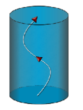
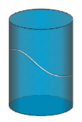
(A)                                                 (B)

Figure 2.2: Timelike and spacelike geodesics. Time goes upward.

Moreover, we can generate new solutions by shifting two of the parameters according to

$$\tau\to\tau+\omega\tau_{ws},\qquad\qquad\qquad\phi\to\phi+\omega\sigma,$$ (2.26)

where $\omega$ is an integer that to some extent can be interpreted as a winding number. The last interpretation comes from the fact that the spectral flow transformation (2.26) gives the two different solutions drawn in Figure 2.3, interpreted as short and long strings wrapping on AdS₃.

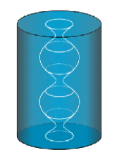
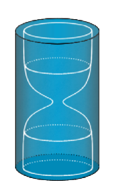
(A)                                               (B)

Figure 2.3: Short and long strings propagating in AdS₃.

From Figure 2.3 (A) we see that timelike spectral flowed geodesics behave as strings contracting and expanding continuously around the axis of the AdS₃ cylinder without ever approaching the boundary. This behavior is due to the opposite forces coming from the tension of the string and the NS-NS $B$ field repulsion. These objects are called short strings. We also have the strings shown in Figure 2.3 (B). They come in from the boundary, shrink around the axis and expand away reaching again the boundary, this are the long strings. The name winding number for the parameter $\omega$ can be misleading, since during the process of collapsing and expanding its value can change.

This concludes our classical analysis of bosonic strings moving on AdS₃. A full quantum approach will be carried off in the next chapters and we will read the previous interpretation in the spectrum of the theory. In chapter 6 we shall see that the fermionic string is still described by a model of this kind.

2.3 The AdS₃/CFT₂ holographic duality

AdS₃/CFT₂ conjecture proposes that superstring theory on AdS₃$\times$S³$\times$T⁴ is dual to a conformal theory leaving on the boundary of AdS₃. This particular realization of the correspondence is especially interesting since, unlike AdS₅/CFT₄, it can be checked beyond the supergravity approximation. This is due to two major facts: $a)$ as we saw, strings on AdS₃ can be described by an exactly solvable conformal theory, ${\it i.e.},$ a WZW model, $b)$ the boundary of the three-dimensional anti-de Sitter space is two-dimensional, giving rise to an infinite number of generators of the conformal group.

In order to make the presentation as clear as possible, we will first restrict to the supergravity regime. Then, for the moment we consider the volume of the compactification manifold of the order of the string length, so we can ignore the Kaluza-Klein modes around these directions and superstring theory reduces to supergravity on AdS₃$\times$S³$\times$${\mathcal{M}}$: (2,0) and (1,1) supergravity for ${\mathcal{M}}=K3$ and T⁴ respectively.

It is known that the low energy dynamics of the D1-D5 system is described by an $U(Q_{1})\times U(Q_{5})$ gauge theory in two dimensions with $\mathcal{N}=(4,4)$ supersymmetry. Moreover, the Higgs branch of this gauge theory description flows in the infrared, ${\it i.e.},$ near the horizon, to an $\mathcal{N}=(4,4)$ super-conformal field theory with central charge $c=6\,Q_{1}Q_{5}$ on certain manifold $\widetilde{\mathcal{M}}$. On the other side, we can think the D1-branes as solitonic strings of the D5-brane theory. These arguments (see [15] for details) led to propose that the conformal theory is a non-linear sigma model on the symmetric orbifold

$$\mathcal{S}^{Q_{1}Q_{5}}({\widetilde{\mathrm{T}}}^{4})=\frac{(\widetilde{\mathrm{T}}^{4})^{Q_{1}Q_{5}}}{\mathcal{S}_{Q_{1}Q_{5}}},$$ (2.27)

where we choose $\widetilde{\mathcal{M}}={\widetilde{\mathrm{T}}}^{4}$, and the tilde on the torus indicates that the four dimensional torus of this theory is not necessarily the same as the one in the bulk theory. $\mathcal{S}_{Q_{1}Q_{5}}$ is the permutation group of $Q_{1}Q_{5}$ variables.

The first evidence for this correspondence comes as usual from the analysis of the symmetries of the bulk theory and the superconformal boundary theory. In the next table we show how the symmetries match.

Bulk IIB SUGRA	Boundary $\mathcal{N}$=(4,4) SCFT
AdS3 isometry $SO(2,2)\,\,\,\,\,\,$	global Virasoro $SL(2,{\mathbb{R}})\times SL(2,{\mathbb{R}})\,\,\,\,\,\,$
S3 isometry $SO(4)$	R-symmetry $SU(2)\times SU(2)$
T4 isometry $SO(4)$	$\widetilde{\mathrm{T}}^{4}$ isometry $SO(4)$
16 supersymmetries	global supercharges

Table 2. Correspondence between the symmetries of the bulk and boundary theory.

Even if a first evidence comes from the matching of the global symmetries on the two sides of the correspondence, the duality should also say something about the more interesting interacting regime. The following formula does the job for AdS₅/CFT₄

$$\mathcal{Z}_{\mathrm{string}}\left[\,\phi|_{\mathrm{boundary}}=\phi_{0}(x)\,\right]=\left\langle e^{\int\,d^{4}x\,\phi_{0}(x)\mathcal{O}(x)}\right\rangle_{\mathrm{CFT}}~{}.$$ (2.28)

Two remarks are in order. The first one is that there is a one to one correspondence between operators $\mathcal{O}(x)$ in the boundary gauge theory and fields $\phi(x_{0},x)$ propagating in the bulk of the AdS₅ space. Secondly, note that in the left hand side of (2.28) the bulk field $\phi(x_{0},x)$ is evaluated in the boundary, $\phi(x_{0},x)\to\phi(x)$. We need to keep in mind these properties while constructing the AdS₃/CFT₂ duality.

Instead of working directly with AdS₃ we will deal with its Euclidean version, the non-compact manifold $H_{3}^{+}=SL(2,C)/SU(2)$, see Section 3.2. We parameterize $H_{3}^{+}$ with the set of coordinates ($\phi,\gamma,\bar{\gamma}$). It is true that this two spaces are related by analytic continuation, nevertheless, some attention should be paid since the WZW model constructed on $SL(2,{\mathbb{R}})$ and on the coset $SL(2,C)/SU(2)$ are not the same. We will point on these differences whenever necessary.

Because $SL(2,C)$ has infinite dimensional representations, it is convenient to introduce a complex variable $x$ (and its conjugate $\bar{x}$), in such a way to encode the components of a given representation in a compact form, specifically, in a function $\Phi_{h,\bar{h}}(\phi,\gamma,\bar{\gamma};x,\bar{x})$. Using these auxiliary variables, it was shown that the $SL(2,C)/SU(2)$ classical theory has the most general solution given by

$$\Phi_{h,\bar{h}}(\phi,\gamma,\bar{\gamma};x,\bar{x})=\frac{1-2h}{\pi}\,\left(e^{-\phi}+(\gamma-x)(\bar{\gamma}-\bar{x})e^{\phi}\right)^{-2h}.$$ (2.29)

It can be shown that near the boundary of AdS₃, ${\it i.e.},$ at $\phi\to\infty$, this function has the same form as the bulk to boundary propagator used in supergravity computations. This identification gives a strong motivation for interpreting $(x,\bar{x})$ as coordinates on the boundary. The charge variables $(x,\bar{x})$ we introduced are fundamental in the approach we use throughout this thesis, so this will be further discussed in the next chapters.

In Table 2 we matched the symmetries on both sides of the AdS₃/CFT₂ correspondence, now we are ready to see the analogue of (2.28). In this case, N-point functions in the Euclidean worldsheet and in the Euclidean boundary conformal theory are believed to be related by

$$\left\langle\prod_{i=1}^{N}\int d^{2}z_{i}\,\Phi_{h_{i}}(z_{i},\bar{z}_{i};x_{i},\bar{x}_{i})\right\rangle_{\Sigma}=\left\langle\prod_{i=1}^{N}\mathcal{O}_{h_{i}}(x_{i},\bar{x}_{i})\right\rangle_{\mathrm{CFT}},$$ (2.30)

where $N$ is the number of insertions and $(x_{i},\bar{x}_{i})$ is identified as the location of the operator $\Phi_{h}$ in the dual boundary theory. In (2.30) there is a one to one correspondence between vertex operators in the worldsheet theory and vertex operators in the boundary theory, $\int d^{2}z\,\Phi_{h_{i}}(z_{i},\bar{z}_{i};x_{i},\bar{x}_{i})\longleftrightarrow\mathcal{O}_{h_{i}}(x_{i},\bar{x}_{i})$. For example, the vertex operator for the graviton corresponds to the energy-momentum tensor of the CFT.

Finally we would like to comment on the fact that in the real AdS₃ with Lorenzian metric, as in other non-compact sigma models, the vertex operators belong to non-unitary representations. This non-unitarity of the model and the analysis of the singularities in the correlation functions show that there is no state/operator correspondence, neither IR/UV relation, unless we extend somehow the concept of state.

2.4 Plane wave limit and BMN conjecture

Originally proposed for the AdS₅/CFT₄ correspondence, the BMN conjecture has attracted a lot of attention, including remarkable developments in the analysis of the AdS₃/CFT₂ case. In few words, the idea of BMN is to take the pp-wave limit on both sides of the duality and see how this affects and possibly reformulate the correspondence. The BMN proposal is a limiting case of the AdS/CFT correspondence, but this should not make us think that the new correspondence is then trivial. As we will see, things are a bit more complicated. This will involve establishing a new operator map and matching the Hilbert spaces on both sides. In the first part of this section we focus on the bulk side and only in the end we sketch the PP-Wave₃/CFT₂ correspondence itself.

Plane-fronted gravitational waves with parallel rays, pp-waves, are defined as spacetime solutions of Einstein equations of motion having a globally constant null Killing vector field $v^{\mu}$, ${\it i.e.},$ it satisfies $\nabla_{\mu}v_{\nu}=0$ and $v_{\mu}v^{\mu}=0$. We will not deal with the most general form of pp-wave backgrounds but instead with a very special type, namely, the ones which have $D$-dimensional metric given by

$$ds^{2}=-2\,du\,dv-\frac{1}{4}\,du^{2}\sum_{I=1}^{D-N-2}\,\mu_{I}^{2}x^{I}x^{I}+\sum_{I=1}^{D-N-2}\,dx^{I}\,dx^{I}+\sum_{i,j=1}^{N}g_{ij}\,dx^{i}\,dx^{j}~{},$$ (2.31)

where $u$ and $v$ are the light-cone directions in spacetime, $\mu$ is certain constant and $g_{IJ}$ is the metric on the transverse directions. The main subject of the discussion will not be affected if we suppose that the internal manifold is the $N$-dimensional torus T^N, so from now on in most of the equations we consider $g_{ij}=\delta_{ij}$, or we simply drop this term. Also notice that in the limit $\mu\to 0$ the pp-wave reduces to the flat space metric.

Another form for the metric can be obtained by changing variables

$$ds^{2}=-2du\,dv-\frac{1}{4}\,du^{2}\sum_{I=2}^{D}\mu_{I}^{2}\,y_{I}\,\bar{y}_{I}+\sum_{I=2}^{D}dy_{I}d\bar{y}_{I}\,.$$ (2.32)

The most interesting property of plane wave geometries is that any spacetime reduces to it in a certain limit. The process is called Penrose limit. The idea is to choose a null geodesic on the given spacetime and zoom into a region very close to it, the spacetime around the chosen point is a plane-wave. Using this procedure we can generate new supergravity backgrounds starting from already known solutions. In particular, we can apply the Penrose modus operandi to the ten-dimensional AdS₅$\times$S⁵ in order to get plane-wave solutions, affecting the AdS/CFT correspondence in a certain way to be clarified. This is exactly what BMN conjecture does. Nevertheless, the fate of holography in this limit is not yet well understood. We hope that with the work done in this thesis we will contribute to understand a little bit better this point (see chapter 5).

Before entering deeper in the BMN proposal, two words on the motivations that brought to it. For a long time it was known that some pp-waves, of the kind used here, were $\alpha^{\prime}$ exact solutions of supergravity theories, ${\it i.e.},$ the pp-wave geometries are supergravity solutions that do not get $\alpha^{\prime}$ corrections. This result led to study strings on pp-waves, supported either by NS-NS or R-R charges, and finally revealing the spectrum in the light-cone gauge. On the other hand, it was shown that in addition to the flat space and AdS₅$\times$S⁵, the Penrose limit of the latter was the only additional maximally supersymmetric solution of type IIB supergravity. Hence, BMN got the main ideas to formulate the PP-Waves/CFT correspondence. Unfortunately, in the light-cone gauge the pp-wave string interactions and the spectrum at $p^{+}=0$ are much harder to determine than it was at first expected (for a review see [20]).

But unlike AdS₅$\times$S⁵, the sigma model for strings moving on AdS₃$\times$S³ with a background NS-NS $B$ field is a well known conformal theory, so it is by itself a natural ground where to test the correspondence beyond the supergravity regime. Furthermore, we do not need to go to the light-cone gauge because the model can be solved in a fully covariant way (see chapter 3). Even more important is that these two properties are preserved in the pp-wave limit. These are the main reasons why in this thesis we will concentrate on this model and thus try to get new insights for the holographic duality, results that then we would like to extend to the more realistic AdS₅/CFT₄.

The Penrose limit of AdS₃$\times$S³ can be carried off choosing a lightlike trajectory moving along the axis of the AdS₃ cylinder and turning around a great circle of S³. This can be performed changing variables in the following way

$$t=\frac{\mu u}{2}+\frac{v}{\mu R^{2}},\qquad\psi=\frac{\mu u}{2}-\frac{v}{\mu R^{2}},\qquad\rho=\frac{r}{R},\qquad\theta=\frac{r_{2}}{R},$$ (2.33)

and taking the limit $R\to\infty$. In the plane wave background the transverse directions are compact with size $\sqrt{\mu p^{+}}$.

We expect that the Penrose limit of a WZW model should give rise to another conformal model. This topic is very important for us and will be discussed widely in the next chapters. What we would like to stress here is that such theories are all generalizations of the more basic Nappi-Witten (NW) model, associated with the central extension of the group $T_{2}\wedge SO(2)$, consisting of translations and rotations in the two-dimensional Euclidean plane.

Appropriately parameterizing the group element and utilizing the Maurer-Cartan formula (2.22) we recover the pp-wave metric in the form (2.32). Moreover, it can be shown that the Nappi-Witten Lie algebra, ${\it i.e.},$ the local behavior of the NW group, is determined by an ${\mathcal{H}}_{4}$ Heisenberg algebra given by [5]

$$[P^{+},P^{-}]=-2i\mu K,\qquad[J,P^{+}]=-i\mu P^{+},\qquad[J,P^{-}]=i\mu P^{-}\,.$$ (2.34)

The generators $P^{\pm}$ stand for the translations in $\mathbb{R}^{2}$, $J$ for the rotation symmetry and $K$ is the central extension element. If we take into account the holomorphic and the anti-holomorphic contributions, it can be shown that the central generator $K=\bar{K}$ is common to both algebras.

This is the simplest of the Heisenberg algebras we can associate to pp-waves backgrounds, in fact, for the most general case (2.31) the ${\mathcal{H}}_{2+2n}$ Heisenberg algebra reads

$$[P^{+}_{i},P^{-}_{j}]=-2i\mu_{i}\delta_{ij}K,\qquad[J,P^{+}_{i}]=-i\mu_{i}P^{+}_{i},\qquad[J,P^{-}_{i}]=i\mu_{i}P^{-}_{i}\,,$$ (2.35)

where $i,j=1,\dots\,2n$. Considering the holomorphic and anti-holomorphic part the total number of generators is $2\,(2+2n)-1$, since as we said above they share the same central element.

Since in the AdS/CFT duality time translation is associated to the dilatation operator, it follows that null geodesics along the axis of the AdS₃ cylinder are related to operators on the boundary with large conformal dimension $\Delta$. On the other hand, fast rotations around the three-sphere imposes large R-charge $J$. Formally, the BMN proposal states that

$$H_{lc}\equiv\partial_{u}=\frac{1}{\mu}\,p^{-}\equiv\Delta-J=\mathrm{fixed}~{},$$ (2.36)

$$P_{lc}\equiv\partial_{v}=p^{+}\equiv\frac{(\Delta+J)}{\mu R^{2}}=\mathrm{fixed}~{}.$$ (2.37)

Operators on the boundary that survive the limit $R\to\infty$ are called BMN operators. Strings propagating in the plane-wave limit of AdS₃$\times$S³ are described by a two-dimensional effective field theory with coupling $g_{2}^{2}=g_{6}^{2}\,(\mu p\,\alpha^{\prime})^{2}$. The coupling of such theory can be written as $J^{2}/N$, that in the double scaling limit $N\to\infty$ and $J\to\infty$ ($J^{2}/N$ kept fixed) differs from the $J^{4}/N^{2}$ dependence of the standard BMN proposal (Penrose limit of AdS₅$\times$S⁵), see [21, 22].

As mentioned earlier, the boundary CFT dual to superstrings on AdS₃$\times$S³$\times$$\mathcal{M}$ is a non-linear $\sigma$-model on the symmetric orbifold $\mathit{Sym}^{N}(\mathcal{M})=(\mathcal{M})^{N}/{\mathcal{S}}_{N}$, where $\mathcal{S}_{N}$ is the symmetric group of $N=Q_{1}Q_{5}$ elements. Following the BMN conjecture, that relates light-cone momenta in the pp-wave background to conformal dimensions and R-charges of the operators in the dual theory, the spectrum of the SCFT was shown to be given by [23]

$$\mathrm{R\!-\!R}:\quad\quad\Delta-J = \sum_{n}N_{n}\,\sqrt{1+\left(\frac{n\,g_{s}\,Q_{5}^{{}^{R}}}{J}\right)^{2}}+g_{s}\,Q_{5}^{{}^{R}}\,\frac{L_{0}^{{}^{\mathcal{M}}}+\bar{L}_{0}^{{}^{\mathcal{M}}}}{J}\,,$$ (2.38)

$$\mathrm{NS\!-\!NS}:\quad\quad\Delta-J = \sum_{n}N_{n}\,\left(1+\frac{n\,Q_{5}^{{}^{NS}}}{J}\right)+Q_{5}^{{}^{NS}}\,\frac{L_{0}^{{}^{\mathcal{M}}}+\bar{L}_{0}^{{}^{\mathcal{M}}}}{J}\,.$$ (2.39)

where R-R and NS-NS stand for the nature of the 3-form flux.

At a first scrutiny, it seemed that the BMN correspondence failed to correctly match the spectra on the two sides, this even for states corresponding to operators with large R-charge. Nevertheless, it has been suggested that this might be due to the fact that the boundary CFT₂ is sitting at the orbifold point, which is not the case for the bulk description. In principle one can dispose of this mismatch by a marginal deformation along the moduli space of the CFT₂. Alternatively one may in principle be able to extrapolate the string spectrum to the symmetric orbifold point and find precise agreement [25, 26, 27].

2.5 The state of the AdS₃/CFT₂ discrepancy

Using standard techniques of super–CFTs on symmetric products $\mathcal{S}^{N}(\mathcal{M})=(\mathcal{M})^{N}/\mathcal{S}_{N}$, the authors of [28] have computed three-point functions of chiral primary operators on the symmetric orbifold (T${}^{4})^{N}/\mathcal{S}_{N}$. On the other hand, in [29] the dual cubic couplings for scalar primaries of type IIB supergravity compactified on T⁴ were found. In this last case, three-point interactions were derived solving the linear equations of motion after a non-trivial redefinition of the fields. In open contradiction with the AdS/CFT proposal, the results found in the two sides disagree. In [30], alternative results from those of [29] are given, but leaving the discrepancy still unsolved. In [30] it is pointed out that maybe there is a problem with the procedure used in [29], specifically, the field redefinition in order to cancel the derivative terms.

In an attempt to clarify this disagreement Lunin and Mathur [31] have developed a novel formulation for computing correlators on the boundary conformal theory. They work directly with the non-abelian permutation group ${\mathcal{S}}_{N}$, instead of the more studied ${\mathbb{Z}}_{N}$. In this new approach, supersymmetric three-point functions reduce to a bosonic contribution times a factor that can be calculated using bosonization representation. It should be stressed that this formalism makes no reference to the specific form of the compact manifold, it only uses the fact that the theory has $\mathcal{N}=(4,4)$ supersymmetry. For the three-point functions they find, remarkably, a result that behaves as the one of [29]. It is also underlined that there is no agreement with [30].

2.5.1 Supergravity in D=6

Supersymmtry in six-dimensions has pseudo Majorana-Weyl spinor supercharges. They can have either positive chirality $Q_{+}^{i}$ $(i=0,1,\dots\,N_{+})$ or negative chirality $Q_{-}^{i}$ $(i=0,1,\dots\,N_{-})$, where $N_{\pm}$ are even numbers. The automorphism group is the symplectic $USp(N_{+})\times USp(N_{-})$.

The supercharges satisfy the anticommutators

$$\{Q_{+}^{i},Q_{+}^{jT}\} = \frac{1}{2}\,(1+\bar{\gamma})\,\gamma^{M}C_{-}P_{M}\Omega^{ij}_{+}~{},$$

$$\{Q_{-}^{i},Q_{-}^{jT}\} = \frac{1}{2}\,(1-\bar{\gamma})\,\gamma^{M}C_{-}P_{M}\Omega^{ij}_{-}~{},$$ (2.40)

$$\{Q_{+}^{i},Q_{-}^{jT}\} = \frac{1}{2}\,(1+\bar{\gamma})\,C_{-}Z^{ij}~{},$$

where $P_{M}$ are the six-dimensional Poincaré generators, $C_{-}$ is the charge conjugation matrix and $Z^{ij}$ are the central charges.

For the theory with $N_{+}=2$ and $N_{-}=0$, the chiral supercharges $Q_{+}^{1,2}$ transform under $USp(2)$. We can double the number of them simply adding another doublet of chiral supercharges, with the composite spinor now transforming under $USp(4)$. If supersymmetry is related to the number of chiral spinors by ${\cal N}=(N_{+}/2,N_{-}/2)$, what we just did can be reread as the extension of chiral ${\cal N}=(1,0)$ to ${\cal N}=(2,0)$. ${\cal N}=(2,0)$ is sometimes called ${\cal N}=4b$ to emphasize that there are four chiral symplectic Majorana-Weyl supercharges.

We are interested in this particular theory since ten-dimensional type IIB supergravity compactified on a four-dimensional manifold $K3$, gives rise to ${\cal N}=(2,0)$ supergravity in six dimensions coupled to $21$ matter tensor multiplets, by definition the latters containing only particles of spin $\leq 1$. Looking at the irreducible representations of the super-Poincaré algebra of ${\cal N}=(2,0)$, we find that there is a graviton $g_{MN}$, four chiral gravitini $\psi_{M}$ and five self-dual two-form fields $B^{i}_{MN}$. On the other hand, each matter multiplet contains an anti-self dual tensor field, four fermions and five scalars. The field content is shown in the next table.

	SUGRA			MATTER
$g_{MN}$	$\psi_{M}$	$B^{i}_{MN}$	$B^{r}_{MN}$	$\chi^{r}$	$\phi^{r}$
1	4	5	1	4	5

Table 3. Field content of pure ${\cal N}=(2,0)$ 6D supergravity and matter multiplets. Indices $i=1,\dots\,5$ transform under the group $SO(5)_{R}$ of the R-symmetry and $r=1,\dots\,n$ is the $SO(n)$ vector index of the rotating tensor multiplet.

In general, chiral superalgebras defined in $D=4k+2$  ($k=0,1,2$)  dimensions possess antisymmetric tensor fields with either  self-dual or anti-self-dual field strengths, $F_{\mu_{1}\dots\,\mu_{2k+1}}=\pm\widetilde{F}_{\mu_{1}\dots\,\mu_{2k+1}}$. The main difficulty raised when constructing a consistent interacting formulation of such theories, in addition to the absence of an explicit action principle, is the mixing of self-dual and anti-self-dual tensor fields by the global $SO(5,n)$. This was solved in [32] noting that in our case the field strengths do not need to have definite duality properties under the $SO(5,n)$ group but only under the local composite $SO(5)\times SO(n)$. This is seen studying the scalar sector of the theory.

It is known that scalar fields in supergravity theories can be described by non-linear sigma models on cosets ${\bf G/H}$, where ${\bf G}$ is the non-compact group of the isometry transformations and ${\bf H}$ is the maximal compact subgroup of ${\bf G}$, called the isotropy group. In the present case, the $5n$ scalars of the theory, five for each matter multiplet, can compactly be encoded in a field $\phi^{ir}$, with $i=1,\dots\,5$ and $r=1,\dots\,n$. These scalars parameterize the $SO(5,n)/\big{(}SO(5)_{R}\times SO(n)\big{)}$ non-linear sigma model. We can regroup them in a $(5+n)\times(5+n)$ vielbein matrix

$$V=\left(\begin{array}[]{cc}u^{i}_{I}&v^{i}_{A}\\ w^{r}_{I}&x^{r}_{A}\\ \end{array}\right)~{},$$ (2.41)

where we have split the $SO(5,n)$ index in $I=1,\dots\,5$ and $A=1,\dots\,n$ for later convinience. The invariant metric of the $SO(5,n)$ manifold is $\eta_{IJ}=\textrm{diag}\,({\mathbb{I}}_{5\times 5},-{\mathbb{I}}_{n\times n})$. As usual the sechsbein $V$ converts curved indices transforming under $SO(5,n)$ into flat indices $i,r$ transforming under the composite local symmetry $SO(5)_{R}\times SO(n)$.

The vacuum has $u^{i}_{I}=\delta^{i}_{I},\,x^{r}_{A}=\delta^{r}_{A},v^{i}_{A}=w^{r}_{I}=0$ and the fluctuations of it away from the identity is given by

$$V^{i}_{I} = \delta^{i}_{I}+\phi^{ir}\delta_{I}^{r}+\frac{1}{2}\phi^{ir}\phi^{jr}\delta_{I}^{j}~{},$$

$$V^{r}_{I} = \delta^{r}_{I}+\phi^{ir}\delta_{I}^{i}+\frac{1}{2}\phi^{ir}\phi^{is}\delta_{I}^{s}~{}.$$ (2.42)

Here we have included second order corrections in order to consider later on cubic couplings of chiral primaries.

We can also define

$$dV\,V^{-1}=\left(\begin{array}[]{cc}Q^{ij}&\sqrt{2}\,P^{is}\\ \sqrt{2}\,P^{jr}&Q^{rs}\\ \end{array}\right)~{},$$ (2.43)

and it can be seen that $Q^{ij}$ and $Q^{rs}$ are the connections of the $SO(5)_{R}$ and $SO(n)$ respectively.

Supersymmetry transformations and field equations for pure ${\cal N}=(2,0)$ supergravity in six dimensions coupled to matter multiplets were derived in [32]. For completeness, we recall a couple of these results. The bosonic field equations are the six-dimensional Einstein equations for the metric

$$R_{MN}=H^{i}_{MPQ}\,{H^{i}_{N}}^{PQ}+H^{r}_{MPQ}\,{H^{r}_{N}}^{PQ}+2{P_{M}}^{ir}\,{P_{N}}^{ir}~{},$$ (2.44)

and the equations for the scalars

$$D^{M}P_{M}^{ir}-\frac{\sqrt{2}}{3}\,H^{i\,MNP}\,H^{r}_{MNP}=0~{},$$ (2.45)

this in addition to the self and anti-self duality conditions for the field strengths $B_{MN}^{i}$ and $B_{MN}^{r}$, respectively. In the fermionic sector we have field equations mixing $\psi_{M}$ and $\chi^{r}$, see for example [33].

Imposing $\langle\psi_{M}\rangle=\langle\chi^{r}\rangle=0\,$ and asking the supersymmetry transformations to vanish in the vacuum, we obtain the Killing spinor equations

$$D_{\mu}\epsilon+\frac{1}{2}\gamma_{\mu}\Gamma^{5}\epsilon=0~{},\qquad D_{a}\epsilon-\frac{i}{2}\gamma_{a}\Gamma^{5}\epsilon=0~{}.$$

In order to determine the spectrum of the theory, fluctuation are linearized according to

$$g_{MN}=\bar{g}_{MN}+h_{MN}~{},\qquad P^{ir}_{M}=\frac{1}{\sqrt{2}}\,\partial_{M}\phi^{ir}~{},\qquad G^{I}=\,dB^{I}=\bar{G}^{I}+g^{I}~{},$$ (2.46)

and first order corrections to the vielbein are considered.

States are classified according to the symmetries of the theory and they are generically written as $D^{[l_{1},l_{2}]}[\Delta_{0},s_{0}][R,S]$. In this notation, $[l_{1},\,l_{2}]$ labels the highest weigh representation of the S³ isometry group $SO(4)_{\rm gauge}$; ($\Delta_{0}$, $s_{0}$), with $\Delta_{0}$ the energy and $s_{0}$ the spin of the lowest energy state, labels the representations of the isometry group $SO(2,2)$ of AdS₃; and, finally, $R$ indicates a representation of the R-symmetry group $SO(4)_{R}$ while $S$ is a generic representation of $SO(n)$.

Since $SO(4)$ is isomorphic to $SU(2)\times SU(2)$ we can rewrite the quantum numbers $l_{1}$ and $l_{2}$ in terms of the spin $SU(2)$s representations

$$[l_{1},l_{2}]~{}\longrightarrow~{}[\,j_{1}=\frac{1}{2}\,(l_{1}+l_{2})\,,\,j_{2}=\frac{1}{2}\,(l_{1}-l_{2})\,]~{}.$$ (2.47)

In the tables 2 and 3 we use the quantum numbers $j_{1}$ and $j_{2}$.

Once we identify the highest spin representation of a multiplet, all the other states follow repeatedly applying the supercharge generators. In [33] it was found that the spin-2 supermultiplet has $D^{[l+1,0]}[l+3,2][0,1]$ as its highest spin state and the spin-1 supermultiplet is generated from $D^{[l+1,-1]}[l+3,1][0,n]$. In order to construct them, the relevant commutators are

$$\left[E,\,Q_{\pm}\right]=\mp\frac{1}{2}\,Q_{\pm}~{},\qquad\left[J,\,Q_{\pm}\right]=-\frac{1}{2}\,Q_{\pm}~{},\qquad\Gamma^{5}Q_{\pm}=\pm Q_{\pm}~{},$$ (2.48)

where $E$ and $J$ are respectively the energy and spin operators of $SO(2,2)$. The former commutation relations tell us that $Q_{-}$ raises the energy and decreases the spin by $\frac{1}{2}$, while $Q_{+}$ decreases both the energy and the spin.

The explicit form of the supercharges is obtained from the Killing spinor equations

$$Q_{\pm}^{[\pm 1/2,-1/2]}\,\left[\mp 1/2,-1/2\right][2_{\pm},0]~{},\qquad~{}~{}\bar{Q}_{\pm}^{[1/2,\pm 1/2]}\,\left[\pm 1/2,1/2\right][2_{\pm},0]~{}.$$ (2.49)

Analogous formulas can be found for the right part. It can be proved that these supercharges in fact generate the $SU(1,1|2)_{L}\oplus SU(1,1|2)_{R}$ superalgebra.

In the next diagrams and tables we show explicitly how the supercharges, acting on the highest spin representations, generate the full supermultiplets. In table 6 we extract from tables 4 and 5 the lowest energy states.

.

Diagram 1. Generation of the spin-2 supermultiplet for $l\geq 0$. The supercharge $Q_{+}$ acts down-left in the diagram and $Q_{-}$ do it in the down-right direction.

$\Delta$	$s_{0}$	$SO(4)_{\mathrm{gauge}}$	$SO(4)_{R}\times SO(n)$	$\left[h,\bar{h}\right]$
$l+3$	$\pm 2$	${\left[\frac{l+1}{2},\frac{l+1}{2}\right]}$	$\left[0,1\right]$	$\frac{\left[l+3\pm 2,l+3\mp 2\right]}{2}$
$l+\frac{5}{2}$	$\pm 3/2$	$\left[\frac{2l+3\pm 1}{4},\frac{2l+3\mp 1}{4}\right]$	$\left[2_{\pm},1\right]$	$\frac{\left[2l+5\pm 3,2l+5\mp 3\right]}{4}$
$l+\frac{7}{2}$	$\pm 3/2$	$\left[\frac{2l+1\pm 1}{4},\frac{2l+1\mp 1}{4}\right]$	$\left[2_{\mp},1\right]$	$\frac{\left[2l+7\pm 3,2l+7\mp 3\right]}{4}$
$l+2$	$\pm 1$	$\left[\frac{2l+2\pm 1}{2},\frac{l+2\mp 1}{2}\right]$	$\left[0,1\right]$	$\frac{\left[l+2\pm 1,l+2\mp 1\right]}{2}$
$l+3$	$\pm 1$	$\left[\frac{l+1\pm 1}{2},\frac{l+1\mp 1}{2}\right]$	$\left[4,1\right]$	$\frac{\left[l+3\pm 1,l+3\mp 1\right]}{2}$
$l+4$	$\pm 1$	$\left[\frac{l\pm 1}{2},\frac{l\mp 1}{2}\right]$	$\left[0,1\right]$	$\frac{\left[l+4\pm 1,l+4\mp 1\right]}{2}$
$l+\frac{5}{2}$	$\pm 1/2$	$\left[\frac{2l+3\pm 3}{4},\frac{2l+3\mp 3}{4}\right]$	$\left[2_{\mp},1\right]$	$\frac{\left[2l+5\pm 1,2l+5\mp 1\right]}{4}$
$l+\frac{7}{2}$	$\pm 1/2$	$\left[\frac{2l+1\pm 3}{4},\frac{2l+1\mp 3}{4}\right]$	$\left[2_{\pm},1\right]$	$\frac{\left[2l+7\pm 1,2l+7\mp 1\right]}{4}$
$l+3$	$\,\,\,\,0$	$\left[\frac{l+1\pm 2}{2},\frac{l+1\mp 2}{2}\right]$	$\left[0,1\right]$	$\frac{\left[l+3,l+3\right]}{2}$

Table 4. Spin-2 supermultiplet tower. The multiplet is organized from the highest spin state to the lowest one. The $SO(4)_{\rm gauge}$ quantum numbers are $[j_{1},j_{2}]$ as defined in (2.47). For each non-scalar field, there is a state with negative spin $s=-s_{0}$, it has same energy $\Delta$ and transforms in the inverse representation of both $SO(4)_{\rm gauge}$ symmetry and $SO(n)$ global group.

.

Diagram 2. Generation of the spin-1 supermultiplet. For the $SO(n)$ singlet $l\geq 0$, whereas the supermultiplet in the vector representation of $SO(n)$ has $l\geq-1$.

$\Delta$	$s_{0}$	$SO(4)_{\mathrm{gauge}}$	$SO(4)_{R}\times SO(n)$	$\left[h,\bar{h}\right]$
$l+3$	$\pm 1$	${\left[\frac{l+1\mp 1}{2},\frac{l+1\pm 1}{2}\right]}$	$\left[0,n\right]$	$\frac{\left[l+3\pm 2,l+3\mp 2\right]}{2}$
$l+\frac{5}{2}$	$\pm 1/2$	$\left[\frac{2l+3\mp 1}{4},\frac{2l+3\pm 1}{4}\right]$	$\left[2_{\pm},n\right]$	$\frac{\left[2l+5\pm 3,2l+5\mp 3\right]}{4}$
$l+\frac{7}{2}$	$\pm 1/2$	$\left[\frac{2l+1\mp 1}{4},\frac{2l+1\pm 1}{4}\right]$	$\left[2_{\mp},n\right]$	$\frac{\left[2l+7\pm 3,2l+7\mp 3\right]}{4}$
$l+2$	$0$	$\left[\frac{l+2}{2},\frac{l+2}{2}\right]$	$\left[0,n\right]$	$\frac{\left[l+2\pm 1,l+2\mp 1\right]}{2}$
$l+3$	0	$\left[\frac{l+1}{2},\frac{l+1}{2}\right]$	$\left[4,n\right]$	$\frac{\left[l+3\pm 1,l+3\mp 1\right]}{2}$
$l+4$	0	$\left[\frac{l}{2},\frac{l}{2}\right]$	$\left[0,n\right]$	$\frac{\left[l+4\pm 1,l+4\mp 1\right]}{2}$

Table 5. Spin-1 supermultiplet tower. In the fourth column, the value of $n$ in $[R,n]$ can be $n=1$ or $n=21$ depending if the multiplet is a singlet or a vector of the global $SO(n)$.

$\Delta$	$s_{0}$	$SO(4)_{\rm gauge}$	$SO(4)_{R}$	$SO(n)$	# dof	6D origin
Non-propagating gravity multiplet $({\bf 3,1})_{S}+({\bf 1,3})_{S}$
$2$	$2$	$\left[0,0\right]$	$\left[0,0\right]$	$1$	$0$	$g_{\mu\nu}$
$\frac{3}{2}$	$\frac{3}{2}$	$\left[0,\frac{1}{2}\right]$	$\left[0,\frac{1}{2}\right]$	$1$	$0$	$\psi_{\mu}$
$1$	$1$	$\left[0,1\right]$	$\left[0,0\right]$	$1$	$0$	$g_{\mu m},B^{5}_{\mu m}$
Spin-$\frac{1}{2}$ hypermultiplet $({\bf 2,2})_{S}$
$1$	$0$	$\left[\frac{1}{2},\frac{1}{2}\right]$	$\left[0,0\right]$	$n$	$4n$	$\phi^{5r},B^{r}_{mn}$
$\frac{3}{2}$	$\frac{1}{2}$	$\left[\frac{1}{2},0\right]$	$\left[0,\frac{1}{2}\right]$	$n$	$4n$	$\chi^{r}$
$2$	$0$	$\left[0,0\right]$	$\left[\frac{1}{2},\frac{1}{2}\right]$	$n$	$4n$	$\phi^{ir}$
Spin-$1$ multiplet $({\bf 3,3})_{S}$
$2$	$0$	$\left[1,1\right]$	$\left[0,0\right]$	$1$	$9$	$B^{5}_{mn},g_{m}{}^{m},g_{\mu}{}^{\mu}$
$\frac{5}{2}$	$\frac{1}{2}$	$\left[1,\frac{1}{2}\right]$	$\left[0,\frac{1}{2}\right]$	$1$	$12$	$\psi_{m}$
$3$	$0$	$\left[\frac{1}{2},\frac{1}{2}\right]$	$\left[\frac{1}{2},\frac{1}{2}\right]$	$1$	$16$	$B^{r}_{mn}$
$3$	$1$	$\left[1,0\right]$	$\left[0,0\right]$	$1$	$3$	$g_{\mu m},B^{5}_{\mu m}$
$\frac{7}{2}$	$\frac{1}{2}$	$\left[\frac{1}{2},0\right]$	$\left[\frac{1}{2},0\right]$	$1$	$4$	$\psi_{m}$
$4$	$0$	$\left[0,0\right]$	$\left[0,0\right]$	$1$	$1$	$g_{m}{}^{m},g_{\mu}{}^{\mu}$

Table 6. Lowest mass spectrum of six-dimensional $N=(2,0)$ supergravity on AdS₃$\times$S³ [34]. From the formula $\Delta(\Delta-2)=M^{2}$ for scalar fields we note the presence of $9+4n$ massless scalars.

2.5.2 The boundary CFT₂

Type IIB superstring on AdS₃ has been proposed to be dual to a CFT theory living on the two-dimensional boundary with $\mathcal{N}=(4,4)$ supersymmetry. For AdS₃$\times$S³$\times$$\mathcal{M}$ the boundary theory is a sigma model whose target space is the symmetric orbifold $(\mathcal{M})^{N}/\mathcal{S}_{N}$. We denote by ${\mathcal{S}}_{N}$ the permutation group of $N$ variables and $N=Q_{1}Q_{5}$, with $Q_{1}$ and $Q_{5}$ respectively the number of fundamental strings and NS5-branes generating the background. The action of the permutation group ${\mathcal{S}}_{N}$ should be understood as the identification of the set of points ($X_{1},\dots,X_{N}$) of the $N$ copies of $\mathcal{M}$ with the other sets of points obtained by permuting in all different ways the $X_{i}^{\prime}\,$s. Similarly for the fermionic coordinates $\psi_{i}$.

The Hilbert space of the orbifold theory $(\mathcal{M})^{N}/\mathcal{S}_{N}$ is obtained as follows [35]. Starting from the Hilbert space H of the CFT on ${\cal M}^{N}$, the action of the discrete group $G\equiv{\cal S}_{N}$ leaves us with the reduced twisted sector $\textsf{H}_{g}$. In addition to this, among all these states we need to keep only those states invariant under the centralizer group $C_{g}$. After these identifications the final Hilbert space of each conjugacy class of $G$ is denoted $\textsf{H}_{g}^{C_{g}}$. Thus, the full Hilbert space of the orbifold theory is

$$\textsf{H}\,\left(\frac{{\cal M}^{N}}{G}\right)=\bigoplus_{[g]}\textsf{H\,}_{g}^{C_{g}}~{},$$ (2.50)

where the sum is over all the different conjugacy classes $[g]$ of $G$.

For the theory here under consideration the discrete symmetry is the permutation group ${\cal S}_{N}$, whose conjugacy classes are characterized by decompositions of the form

$$[g]=(1)^{N_{1}}\dots\,(s)^{N_{s}}~{},$$ (2.51)

where $(n)$ is the number of elements that are permuted and $N_{n}$ is the number of times this operation is carried off. For a system with $N$ elements it is clear that $\sum_{n}\,nN_{n}=N$. This decomposition of the conjugacy classes is useful since we can identify the centralizer group as

$$C_{g}=S_{N_{1}}\times(S_{N_{2}}\times\mathbb{Z}_{2}^{N_{2}})\times\cdots\times(S_{N_{s}}\times\mathbb{Z}_{s}^{N_{s}})~{}.$$ (2.52)

In this notation, a generic $S_{N_{n}}$ permutes the sets of $(n)$ elements, while $Z_{n}$ acts on the internal elements of $(n)$. Now we can decompose the twist sector in smaller Hilbert spaces $\textsf{H\,}^{\mathbb{Z}_{n}}_{(n)}$ invariant under the action of $\mathbb{Z}_{n}$, such that

$$\textsf{H}\,({\cal S}^{N}{\cal M})=\bigoplus_{\sum nN_{n}}~{}\bigotimes_{n>0}\,{\cal S}^{N_{n}}\,\textsf{H\,}_{(n)}^{\mathbb{Z}_{n}}~{}.$$ (2.53)

Hence, the spectrum of CFTs on symmetric products ${\cal M}^{N}/{\cal S}_{N}$ is build by the action of $\mathbb{Z}_{n}$–twist fields ($n=1,\dots\,N$) on the vacuum of the theory [36].

From the point of view of the CFT₂ the action of the permutation group is realized by twist fields $\sigma_{n}$, for permutations of length $n$, acting on the $N$ copies of $c=6$ theories. If we suppose the theory defined on a cylinder, we can see the twist operator $\sigma_{n}$ as linking $n$ conformal field theories defined on each $\mathcal{M}$ in such a way that the final CFT lives in a circle that is $n$ times larger than the initial one. The vacuum energy difference tells us that the twist field $\sigma_{n}$ has conformal dimension $\Delta_{n}={\frac{1}{4}}\,(n-\frac{1}{n})$. Note that even if the sample twist operator $\sigma_{n}$ is the building block of the symmetric orbifold theory, and we will deal mostly with it, it should be kept in mind that in fact there is one twist operator for each conjugacy class, and not for a simple element of the group, see (2.53). CFT operators have the form [31]

$${\cal O}_{n}=\frac{c_{n}}{N!}\sum_{h\in S_{N}}\sigma_{hnh^{-}1}~{},$$ (2.54)

where $c_{n}$ is a normalization constant. Moreover, we should consider twist operators with all possible length $\sigma_{n}$ with $n=1,\dots\,N$, and symmetrize in all different ways. In the correlation functions a simple global combinatorial factor will take into account this fact.

The match of the symmetries on both sides of the AdS₃$\times$S³/CFT₂ correspondence tells us that the isometry group $SO(4)$ of the three-sphere should be identified with a pair of $SU(2)$ algebras, left and right, corresponding to the R-symmetry of the $\mathcal{N}=(4,4)$ boundary theory. Thus, a string moving around S³ has an angular momentum that is naturally associated to the R-charge of certain operator on the boundary. Hence it follows that high angular momenta are dual to operators with large R-charge. In the boundary theory we will only consider chiral primary operators.

Chiral primary operators (CPO) are operators on the super–CFT that are annihilated by half of the supersymmetries and have same conformal dimension and R-charge, $h=j$. Since the twist fields we defined above only permute copies of $\mathcal{M}$ and do not carry any charge, we see that in general the twist $\sigma_{n}$ is not a CPO, except for the trivial $n=1$. In order to provide the twist operator with R-charge, we define the following currents of the $SU(2)_{L}$ ${\cal N}=(4,4)$ automorphism

$$J_{-m/n}^{+}\equiv\oint\frac{dz}{2\pi i}\sum_{k=1}^{n}J_{z}^{k,+}(z)\,e^{-2\pi im(k-1)/n}z^{-m/n}~{},$$ (2.55)

where $k$ labels the copy of $\cal M$ and the integral goes around the origin of the $z$-plane. Acting with these currents on a twist operator the conformal dimension get increased by $m/n$ while the charge is raised by one unit. Choosing $m/n<1$ we can repeatedly apply the currents until we reach the point where the equality $h=j$ holds, corresponding to the chiral primaries.

It is useful to define the local map $z\to at^{n}$, which states that the $n$ copies of $\mathcal{M}$ involved in the twist operation are translated into a single copy on the covering space $\Sigma$. In this space, that we call $t$-space in order to distinguish it from the original $z$-plane, $n$ different currents give rise to a single current on the covering space. After mapping we define the currents in the $t$-space as

$$J_{-m}^{+}\equiv\int\frac{dt}{2\pi i}\,J_{t}^{+}(t)\,t^{-m}~{}.$$ (2.56)

Denoting the R-charged twist fields as $\sigma_{n}^{\pm}$ and using the $t$-space notation above introduced, it is easy to see that we can construct the following chiral operators

$$|\sigma_{n}^{-}\rangle\equiv J_{-(n-2)}^{+}\cdots J_{-3}^{+}J_{-1}^{+}|\,0^{-}\rangle_{NS}~{},\qquad\mathrm{with}\qquad h=j=\frac{n-1}{2}~{},$$ (2.57)

and

$$|\sigma_{n}^{+}\rangle\equiv J_{-n}^{+}J_{-(n-2)}^{+}\cdots J_{-3}^{+}J_{-1}^{+}|\,0^{-}\rangle_{NS}~{},\qquad\mathrm{with}\qquad h=j=\frac{n+1}{2}~{}.$$ (2.58)

These relations are valid only for $n$ odd. In fact, in the covering space $\Sigma$ the spinor coordinates are identified according to $\psi_{t}(t)\to(-1)^{n-1}\psi_{t}(t)$, so for $n$ even the spinor is antiperiodic around $t=0$. The corresponding Ramond vacua are of two types, depending on their $J^{3}$ charge. We can have $|\,0^{+}\rangle_{R}$ or $|\,0^{-}\rangle_{R}$, both of them with $h=\frac{1}{4}$, but $j=\pm\frac{1}{2}$ respectively. The Ramond vacua are related between them by $|\,0^{+}\rangle_{R}=J_{0}^{+}|\,0^{-}\rangle_{R}$, and to the Neveu-Schwarz vacuum by spectral flow transformation. From the worldsheet point of view, the field we should insert in $t=0$ in order to pass from one type of vacuum to the other is the spin field, $|\,0^{\pm}\rangle_{R}=S^{\pm}|\,0\rangle_{NS}$. The chiral primaries are in this case defined as

$$|\sigma_{n}^{-}\rangle\equiv J_{-(n-2)}^{+}\cdots J_{-2}^{+}J_{0}^{+}|\,0^{-}\rangle_{R}~{},\quad|\sigma_{n}^{+}\rangle\equiv J_{-n}^{+}J_{-(n-2)}^{+}\cdots J_{-2}^{+}J_{0}^{+}|\,0^{-}\rangle_{R}~{},$$ (2.59)

with the same conformal dimension, and charge, as $n$ odd. We can now put together left and right movers in order to write the complete chiral primaries of the orbifold theory

$$\sigma_{n}^{\pm\pm}~{},\qquad\mathrm{with}\qquad h=\bar{h}~{},$$ (2.60)

and

$$\sigma_{n}^{\pm\mp}~{},\qquad\mathrm{with}\qquad h=\bar{h}\pm 1~{}.$$ (2.61)

Chapter 3 Bosonic String Amplitudes on AdS₃$\times$S³ and the PP-Wave Limit

In this chapter we examine the quantum properties of bosonic strings living on AdS₃$\times$S³ with NS-NS three-form flux background. First we review the main properties of the affine algebras associated to this background and then we generate the spectrum, identifying at a quantum level the short and long strings introduced in the previous chapter. In the last part we turn to the charge variables formulation of the theory and comment further on the holographic screen of section 2.3, an approach that will reveal all its power only in the last chapter. After this we pass to the main goal, namely, to prove that we can explicitly compute correlation functions in the plane wave limit starting from the correlators of primary fields of $\widehat{SL}(2,\mathbb{R})$ and $\widehat{SU}(2)$. This chapter is in part based on results published in [2].

3.1 Affine algebras and spectra

Affine conformal models are two dimensional field theories that, in addition to the conformal invariance we are use to, shows a chiral symmetry in some primary fields with unit weight. These fields are the so called affine currents. In other words, the standard Virasoro generators are supplemented by a set of chirally conserved currents, ${\it i.e.},$ they fulfil $\bar{\partial}J=0$. In section 2.2 we showed that this is the chief property of WZW models describing strings on group manifolds, see (2.20) and (2.21). In particular this is true for strings living on AdS₃ and S³, so it is fundamental for us to understand in detail how these models work.

Affine Kac-Moody algebras by definition meet conformal and chiral invariance, so the currents are constraint to have operator product expansion (OPE) given by

$$\mathcal{J}^{i}(z)\,\mathcal{J}^{j}(w)\sim\displaystyle\frac{k\,g^{ij}}{(z-w)^{2}}+i\,f^{ijk}\frac{\mathcal{J}^{k}(w)}{z-w},$$ (3.1)

where $k$ is a positive integer known as the level of the algebra. Notice that the general metric $g$ has upper indices and it is symmetric on their interchange.

Expanding in Laurent modes $\mathcal{J}^{i}(z)=\sum_{n\in\,\mathbb{Z}}\mathcal{J}_{n}^{i}\,z^{-n-1}$ and integrating in the complex plane it is straightforward to get the commutation relation of the currents

$$[\mathcal{J}^{i}_{n},\,\mathcal{J}^{j}_{m}]=\,k\,n\,g^{ij}\,\delta_{n+m,0}+i\,f^{ijk}\mathcal{J}^{k}_{n+m}~{}.$$ (3.2)

This is the Affine Kac-Moody algebra. This algebra is an infinite-dimensional extension of ordinary Lie algebras (infinite generators since $-\infty<n<\infty$). The subalgebra of zero modes $\mathcal{J}_{0}^{i}$ is known as the horizontal Lie algebra in which the central extension $k$ is absent. Moreover, from this general form we can see that the $f^{ijk}$ coefficients are no more than the structure constant of the finite-dimensional Lie algebra (the zero mode algebra of the currents). As we are dealing with two algebras, the algebra on the target space and the current algebra on the worldsheet, we will distinguish them by putting a hat on the latter. We will also restrict our presentation only to $\widehat{SL}(2,{\mathbb{R}})$ and $\widehat{SU}(2)$ since these are the current algebras associated with strings moving on AdS₃$\times$S³ with NS-NS two form field $B$.

Due to the fact that $\widehat{SL}(2,{\mathbb{R}})$ and $\widehat{SU}(2)$ are analytical continuation of each other, it is not surprising that the algebras and other relations in the two cases have similar expressions. Thus in order to avoid repetitions we will use the letter $\mathcal{J}$ for the generators of both algebras and agree that the upper signs in the following equations correspond to $\widehat{SL}(2,{\mathbb{R}})$ and the lower ones to $\widehat{SU}(2)$. For the moment we also suppose that they have same level $k$.

The current algebras have the same form as given in (3.1) with $i,j,k=1,2,3$, in accordance with the number of generators. Moreover $g_{ij}=\eta_{ij}=\textrm{diag}\,(++-)$ for $\widehat{SL}(2,{\mathbb{R}})$ and $g_{ij}=\delta_{ij}=\textrm{diag}\,(+++)$ for $\widehat{SU}(2)$. If we now define the conventional operators $\mathcal{J}^{\pm}=\mathcal{J}^{1}\pm i\mathcal{J}^{2}$, we get the OPEs

$$\mathcal{J}^{+}(z)\,\mathcal{J}^{-}(w) \sim \frac{k}{(z-w)^{2}}\mp\frac{2\mathcal{J}^{3}(w)}{z-w}\ ,$$

$$\mathcal{J}^{3}(z)\,\mathcal{J}^{\pm}(w) \sim \pm\frac{\mathcal{J}^{\pm}(w)}{z-w}\ ,$$

$$\mathcal{J}^{3}(z)\,\mathcal{J}^{3}(w) \sim \displaystyle\mp\frac{k}{2(z-w)^{2}}\ .$$ (3.3)

This set of OPEs are essential for our approach and will be used intensely throughout this thesis. From here we can read the explicit $\widehat{SL}(2,{\mathbb{R}})$ and $\widehat{SU}(2)$ OPEs or commutators. If needed, the formulas are given in (4.1) and (4.9).

Expanding in modes, the analogue of (3.2) for $i,j,k=\pm,3$ is

$$\left[\mathcal{J}_{n}^{+},\,\mathcal{J}_{m}^{-}\right] = kn\,\delta_{n+m,0}\mp 2\mathcal{J}_{n+m}^{3}~{},$$

$$\left[\mathcal{J}_{n}^{3},\,\mathcal{J}_{m}^{\pm}\right] = \pm\mathcal{J}_{n+m}^{\pm}~{},$$

$$\left[\mathcal{J}_{n}^{3},\,\mathcal{J}_{m}^{3}\right] = \mp\frac{k}{2}\,n\delta_{n+m,0}~{}.$$ (3.4)

Non-singularity of the fields $\mathcal{J}^{i}(z)$ at $z=0$ imposes the existence of states $|\,R_{i}\rangle$ that are annihilated by the positive modes of the currents, ${\it i.e.},$ ${\mathcal{J}}_{n}^{i}|\,R_{i}\rangle=0$ for $n\geq 0\,$. This defines the primary states or highest weight states. Here we have assumed that all these states $|\,R_{i}\rangle$ transform in some representation $R$ of the horizontal algebra, that is $\mathcal{J}_{0}^{i}\,|\,R_{i}\rangle=\,(T^{i}_{R})_{ij}\,|\,R_{j}\rangle$, where $T^{i}$ are the generators. The OPE counterpart of this relation is

$$\mathcal{J}^{i}(z)R_{i}(w)\sim\frac{{T_{R}^{i}}_{ij}}{z-w}\,R_{j}(w)\,,$$ (3.5)

where the fields above defined act on the vacuum of the theory as $R_{i}(0)|\,0\rangle\equiv|\,R_{i}\rangle$. The fields $R_{i}(z)$ are in consequence called affine primaries.

To construct the spectrum of the theory we start from the vacuum states and apply repeatedly the raising operators with negative modes $\mathcal{J}_{n<0}^{\pm,3}\,\,$. At this point a comment is in order: the spectrum of strings on AdS₃, or, equivalently, the representations of $SL(2,\mathbb{R})$, contain ghosts (the generators $\mathcal{J}^{3}$ create states with negative norm); making the theory ill-defined. This longstanding problem was solved in [19], where the authors proved a no-ghost theorem for the model making use of extra unexpected states. These states arise as representations of the spectral flowed algebra. We will come back to this further down.

The Sugawara construction establishes that the energy-momentum tensor can be written as a bilinear in the currents

$$T(z)=\frac{1}{k\mp 2}\left[\frac{1}{2}\,(\mathcal{J}^{+}\mathcal{J}^{-}+\mathcal{J}^{-}\mathcal{J}^{+})\mp\mathcal{J}^{3}\mathcal{J}^{3}\right]~{}.$$ (3.6)

Expanding in modes we get the Virasoro generators

$$L_{n\neq o}=\frac{1}{k\mp 2}\sum_{m=1}^{\infty}(\mathcal{J}_{n-m}^{+}\mathcal{J}_{m}^{-}+\mathcal{J}_{n-m}^{-}\mathcal{J}_{m}^{+}\mp 2\mathcal{J}_{n-m}^{3}\mathcal{J}_{m}^{3})~{}.$$ (3.7)

As usual, $L_{0}$ is ambiguous under normal ordering, so we define

$$L_{0}=\frac{1}{k\mp 2}\,\left[\,\frac{1}{2}\,(\mathcal{J}_{0}^{+}\mathcal{J}_{0}^{-}+\mathcal{J}_{0}^{-}\mathcal{J}_{0}^{+})\mp(\mathcal{J}_{0}^{3})^{2}+\sum_{m=1}^{\infty}(\mathcal{J}_{-m}^{+}\mathcal{J}_{m}^{-}+\mathcal{J}_{-m}^{-}\mathcal{J}_{m}^{+}\mp 2\mathcal{J}_{-m}^{3}\mathcal{J}_{m}^{3})\,\right]~{}.$$ (3.8)

For convenience we remember the Virasoro algebra

$$[L_{n},L_{m}]=(n-m)L_{n-m}+\frac{c}{12}\,(n^{3}-n)\,\delta_{n+m,0}~{}.$$ (3.9)

Note that the affine current algebra is larger than the conformal Virasoro algebra since it comprises conformal and chiral invariance. That is why the Virasoro generators can be expressed in terms of the modes of the currents. The central extension parameter $k$ of Kac-Moody algebras and the central extension of the Virasoro algebra are related by

$$c=\frac{3k}{k\mp 2}~{}.$$ (3.10)

The generators of both algebras have commutator $[L_{n},\mathcal{J}_{m}^{i}]=-m\,\mathcal{J}_{m+n}^{i}$.

The Casimir operator of the group is defined by

$$\vec{\mathcal{J}}^{\,2}=(k\mp 2)\,L_{0}=\frac{1}{2}\,(\mathcal{J}_{0}^{+}\mathcal{J}_{0}^{-}+\mathcal{J}_{0}^{-}\mathcal{J}_{0}^{+})\mp(\mathcal{J}_{0}^{3})^{2}~{}.$$ (3.11)

For $\widehat{SL}(2,\mathbb{R})$ we have three types of unitary normalizable representations [39]:

1) Lowest-weight discrete representations ${\cal D}^{+}_{l}$, constructed starting from a state $|l\rangle$ which satisfies $K^{-}|l\rangle=0$, with $l>1/2$. The spectrum of $K^{3}$ is given by $\{l+n\}$, $n\in\mathbb{N}$ and the Casimir is ${\cal C}_{SL}=-l(l-1)$.

2) Highest-weight discrete representations ${\cal D}^{-}_{l}$, constructed starting from a state $|l\rangle$ which satisfies $K^{+}|l\rangle=0$, with $l>1/2$. The spectrum of $K^{3}$ is given by $\{-l-n\}$, $n\in\mathbb{N}$ and the Casimir is ${\cal C}_{SL}=-l(l-1)$.

3) Continuous representations ${\cal C}_{l,\alpha}$, constructed starting from a state $|l,\alpha\rangle$ which satisfies $K^{\pm}|l,\alpha\rangle\neq 0$, with $l=1/2+i\sigma$, $\sigma\geq 0$. The spectrum of $K^{3}$ is given by $\{\alpha+n\}$, $n\in\mathbb{Z}$ and $0\leq\alpha<1$. The Casimir is ${\cal C}_{SL}=1/4+\sigma^{2}$.

Other representations come from the spectral flow [19, 38]

$$\mathcal{J}^{3}_{n}\, \longrightarrow \,\widetilde{\mathcal{J}}_{n}^{3}\,=\mathcal{J}_{n}^{3}-\frac{k}{2}\,w\,\delta_{n,0}~{},$$

$$\mathcal{J}^{+}_{n}\, \longrightarrow \,\widetilde{\mathcal{J}}_{n}^{+}=\mathcal{J}_{n+w}^{+}~{},$$ (3.12)

$$\mathcal{J}^{-}_{n}\, \longrightarrow \,\widetilde{\mathcal{J}}_{n}^{-}=\mathcal{J}_{n-w}^{-}~{}.$$

For the Virasoro generators the automorphism acts as

$$L_{n}\,\longrightarrow\,\widetilde{L}_{n}=L_{n}+w\,{\mathcal{J}}^{3}_{n}-\frac{k}{4}\,w^{2}\delta_{n,0}~{}.$$ (3.13)

The full spectrum includes the representations of these spectral flowed algebras, ${\it i.e.},$ representations builded from a general highest weight state $|\,h;\omega\rangle$.

The representations of the spectral flow algebras $\mathcal{D}_{l}^{\omega}$ and $\mathcal{C}_{l,\alpha}^{\omega}$ are generated applying on the spectral flowed highest weight states the currents of $\widehat{SL}(2,\mathbb{R})$. For discrete representations these they are defined as

$$K_{n+\omega}^{+}|\,h;\omega\rangle=0,\qquad K_{n-\omega-1}^{-}|\,h;\omega\rangle=0,\qquad K_{n}^{3}|\,h;\omega\rangle=0,\qquad n=1,2,\dots$$ (3.14)

and for continuous representations

$$K_{n\pm\omega}^{\pm}|\,h,\alpha;\omega\rangle=0,\quad\qquad K_{n}^{3}|\,h,\alpha;\omega\rangle=0,\qquad n=1,2,\dots$$ (3.15)

Since irreps with different $w$ are not equivalent, the full Hilbert space including spectral flowed representations is

$${\mathsf{H}}_{SL(2,\mathbb{R})}=\oplus_{w=-\infty}^{\infty}\left[\,\left(\,\int_{\frac{1}{2}}^{\frac{k-1}{2}}dl\,\,\mathcal{D}_{l}^{\omega}\otimes\bar{\mathcal{D}}_{l}^{\omega}\,\right)\oplus\left(\,\int_{\frac{1}{2}+i{\mathbb{R}}}dl\int_{0}^{1}d\alpha\,\,\mathcal{C}_{l,\alpha}^{\omega}\otimes\bar{\mathcal{C}}_{l,\alpha}^{\omega}\,\right)\,\right]\,\,.$$ (3.16)

The analysis of the spectrum leads to identify the continuous representations, whith discrete energies, with short strings moving deeply inside AdS₃ (see section 2.2). In [19] it was shown that the spectral flow of continuous representations lead to physical states with energy given by

$$E=\frac{kw}{2}+\frac{1}{w}\,\left[\,2\,\frac{s^{2}+\frac{1}{4}}{k-2}+\bar{N}+N+\Delta_{int}+\bar{\Delta}_{int}-2\,\right]~{},$$ (3.17)

where $N$ is the number of current excitations, left and right contributions are considered, before the spectral flow is taken. These new states with continuous energies represent the long strings also discussed in section 2.2.

For $SU(2)$ the things are much simpler since we have only one type of unitary representations ${V}_{\tilde{l}}$ with $2\tilde{l}\in\mathbb{N}$, $\tilde{m}=-\tilde{l},-\tilde{l}+1,...,\tilde{l}$ and the spectral flow operation does not give extra states but only maps between conventional representations. Thus, the full Hilbert space in this case is

$${\mathsf{H}}_{SU(2)}=\oplus\,{}_{\tilde{l}=0,\frac{1}{2}\dots\,\frac{k}{2}}V_{\tilde{l}}\,\otimes\,{\bar{V}_{\tilde{l}}}~{}.$$ (3.18)

3.2 Penrose limit of amplitudes on AdS₃$\times$S³

Starting from three-point correlators for vertex operators of strings on AdS₃$\times$S³, in this section we proceed to determine the corresponding correlators in the plane wave background. The novelty of our approach is that the Penrose limit is taken scaling the charge variables already introduced for $SL(2,\mathbb{R})$ [40] and similar for $SU(2)$. The limit of the $SU(2)$ three-point couplings [41] has been considered in [5] and we refer to that paper for a detailed discussion. Here we provide a similar analysis for the $SL(2,\mathbb{R})$ structure constants and show that when combined with the $SU(2)$ part they reproduce in the limit the $\widehat{\cal H}_{6}$ structure constants we will see in chapter 4. As a first step, we begin by introducing the irreps of the Heisenberg algebra $\mathcal{H}_{6}$ and then show how the quantum numbers of the two models before and after the Penrose limit are related to each other. But, first of all let us clarify the role of the Euclidean AdS₃ (see also section 2.3).

In general, the AdS₃/CFT₂ correspondence entails the exact equivalence between superstring theory on AdS₃$\times$${\cal M}$, where ${\cal M}$ is some compact space represented by a unitary CFT on the worldsheet, and a CFT defined on the boundary of AdS₃. Equivalence at the quantum level implies a isomorphism of the Hilbert spaces and of the operator algebras of the two theories. For various reasons it is often convenient to consider the Euclidean version of AdS₃ described by an $SL(2,\mathbb{C})/SU(2)$ WZW model on the hyperbolic space $H^{+}_{3}$ with $S^{2}$ boundary, see section 2.3. Although the Lorentzian $SL(2,\mathbb{R})$ WZW model and the Euclidean $SL(2,\mathbb{C})/SU(2)$ WZW model are formally related by analytic continuation of the string coordinates, their spectra are not the same. As observed in [19, 10], except for unflowed ($w=0$) continuous representations, physical string states on Lorentzian AdS₃ corresponds to non-normalizable states in the Euclidean $SL(2,\mathbb{C})/SU(2)$ model. Yet unitarity of the dual boundary CFT₂ that follows from positivity of the Hamiltonian and slow growth of the density of states should make the analytic continuation legitimate. Indeed correlation functions for the Lorentzian $SL(2,\mathbb{R})$ WZW model have been obtained by analytic continuation of those for the Euclidean $SL(2,\mathbb{C})/SU(2)$ WZW model [10]. Singularities displayed by correlators involving non-normalizable states have been given a physical interpretation both at the level of the worldsheet, as due to worldsheet instantons, and of the target space. Some singularities have been associated to operator mixing and other to the non-compactness of the target space of the boundary CFT₂. The failure of the factorization of some four-point string amplitudes has been given an explanation in [10] and argued not to prevent the validity of the analytic continuation from Euclidean to Lorentzian signature. Since we are going to take a Penrose limit of $SL(2,\mathbb{R})$ correlation functions computed by analytic continuation from $SL(2,\mathbb{C})/SU(2)$, we need to assume the validity of this procedure. Reversing the argument, the agreement we found between correlation functions in the Hpp-wave computed by current algebra techniques with those resulting from the Penrose limit (current contraction) of the $SL(2,\mathbb{C})/SU(2)$ WZW model should be taken as further evidence for the validity of the analytic continuation.

To discuss how the three-point couplings in the Hpp-wave with ${\mathcal{H}}_{6}^{L}\times\mathcal{H}_{6}^{R}$ symmetry are related to the three-point couplings in AdS₃$\times$S³, the first thing we have to understand is how the ${\mathcal{H}}_{6}$ representations arise in the limit from representations of $SL(2,\mathbb{R})\times SU(2)$. In the next chapter we will examine in more details ${\mathcal{H}}_{6}$, here we just want to underline that as much as for $SL(2,\mathbb{R})\,$, $\mathcal{H}_{6}$ has three types of representations: discrete irreps $V^{\pm}_{p,\hat{\jmath}}$ and continuous ones $V^{0}_{s_{1},s_{2},\hat{\jmath}}$ , where $p,s$ and $\hat{\jmath}$ are the quantum numbers labelling the representations.

Let us start with the $V^{+}_{p,{\hat{\jmath}}}$ representations. Following [5] we consider states that sit near the top of an $SU(2)$ representation

$$\tilde{l}=\frac{k_{2}}{2}\mu_{2}p-b\ ,\hskip 28.45274pt\tilde{m}=\frac{k_{2}}{2}\mu_{2}p-b-n_{2}\ .$$ (3.19)

In order to get in the limit states with a finite conformal dimension and well defined quantum numbers with respect to the currents in $(\ref{contr})$, we have to choose for $SL(2,\mathbb{R})$ a ${\cal D}^{-}_{l}$ representation with

$$l=\frac{k_{1}}{2}\mu_{1}p-a\ ,\hskip 28.45274ptm=-\frac{k_{1}}{2}\mu_{1}p+a-n_{1}\ .$$ (3.20)

In the limit ${\hat{\jmath}}=-\mu_{1}a+\mu_{2}b$.

Reasoning in a similar way one can see that the $V^{-}_{p,{\hat{\jmath}}}$ representations result from ${\cal D}^{+}_{l}\times V_{\tilde{l}}$ representations with

$$l = \frac{k_{1}}{2}\mu_{1}p-a\ ,\hskip 28.45274ptm=\frac{k_{1}}{2}\mu_{1}p-a+n_{1}\ ,$$

$$\tilde{l} = \frac{k_{2}}{2}\mu_{2}p-b\ ,\hskip 28.45274pt\tilde{m}=-\frac{k_{2}}{2}\mu_{2}p+b+n_{2}\ ,$$ (3.21)

and ${\hat{\jmath}}=\mu_{1}a-\mu_{2}b$ in the limit.

Finally the $V^{0}_{s_{1},s_{2},{\hat{\jmath}}}$ representations result from ${\cal D}^{0}_{l,\alpha}\times V_{\tilde{l}}$ representations with

$$l=\frac{1}{2}+i\sqrt{\frac{k_{1}}{2}}s_{1}\ ,\hskip 11.38092ptm=\alpha+n_{1}\ ,\hskip 11.38092pt\tilde{l}=\sqrt{\frac{k_{2}}{2}}s_{2}\ ,\hskip 11.38092pt\tilde{m}=n_{2}\ ,$$ (3.22)

and ${\hat{\jmath}}=-\mu_{1}\alpha$. As we shall see the tensor product of these representations reproduces in the limit for ${\mathcal{H}}_{6}$, see Eq. $(\ref{tensorH6})$.

We introduce a vertex operator for each unitary representations of $SL(2,\mathbb{R})$

$$\Psi^{+}_{l}(z,x) = \sum_{n=0}^{\infty}c_{l,n}(-x)^{n}R^{+}_{l,n}(z)\ ,$$

$$\Psi^{-}_{l}(z,x) = \sum_{n=0}^{\infty}c_{l,n}x^{-2l-n}R^{-}_{l,n}(z)\ ,$$

$$\Psi^{0}_{l,\alpha}(z,x) = \sum_{n\in\mathbb{Z}}x^{-l+\alpha+n}R^{0}_{l,\alpha,n}(z)\ ,$$ (3.23)

where we denote by $R$ the modes of the primary in the $n$ basis and $c_{l,n}^{2}=\frac{\Gamma(2l+n)}{\Gamma(n+1)\Gamma(2l)}$.

As we anticipated in section 2.3, we can define a two-dimensional holographic screen where the CFT lives. This space is parameterize by the charge variables $(x,\bar{x})$ that are identified as the points where the boundary operators are inserted. Using this variables we can identify the action of the currents of $SL(2,\mathbb{R})$ on the affine primaries with some differential operators defined on the $x$ space. Specifically we can establish the relation

$$K^{A}(z)\Psi_{l}(w,\bar{w};x,\bar{x})\sim\frac{\mathcal{D}^{A}}{z-w}\,\Psi_{l}(w,\bar{w};x,\bar{x}),\qquad A=\pm,3$$ (3.24)

considering the following differential operators

$${\cal D}_{1}^{-}=-x^{2}\partial_{x}-2lx\ ,\hskip 11.38092pt{\cal D}_{1}^{+}=-\partial_{x}\ ,\hskip 11.38092pt{\cal D}_{1}^{3}=l+x\partial_{x}\ .$$ (3.25)

Similarly for $S^{3}$ we introduce

$$\Omega_{\tilde{l}}(z,y)=\sum_{m=-\tilde{l}}^{\tilde{l}}\tilde{c}_{\tilde{l},m}y^{\tilde{l}+m}R_{\tilde{l},m}(z)\ ,\\$$ (3.26)

where $\tilde{c}_{\tilde{l},m}^{2}=\frac{\Gamma(2\tilde{l}+1)}{\Gamma(\tilde{l}+m+1)\Gamma(\tilde{l}-m+1)}$ and the differential operators that represent the $SU(2)$ action are

$${\cal D}_{2}^{+}=\partial_{y}\ ,\hskip 11.38092pt{\cal D}_{2}^{-}=-y^{2}\partial_{y}+2\tilde{l}y\ ,\hskip 11.38092pt{\cal D}_{2}^{3}=y\partial_{y}-\tilde{l}\ .$$ (3.27)

Generalizing the case studied in [5], we can now implement the Penrose limit on the operators $\Psi^{a}_{l}(z,x)\Omega_{\tilde{l}}(z,y)$ and determine their precise relation with the primaries $\Phi^{a}(z,x,y)$ of the Heisenberg algebra $\widehat{\cal H}_{6}$ coming from the Penrose limit. In this section we introduce two charge variables for $\widehat{\cal H}_{6}$, denoted by $x$ and $y$ in order to emphasize that they are related to the charge variables of $SL(2,\mathbb{R})$ and $SU(2)$ respectively.

For the discrete representations we have

$$\Phi^{+}_{p,\hat{\jmath}}(z,x,y) = \lim_{k_{1},k_{2}\to\infty}\left(\frac{x}{\sqrt{k_{1}}}\right)^{-2l}\left(\frac{y}{\sqrt{k_{2}}}\right)^{2\tilde{l}}\Psi^{-}_{l}\left(z,\frac{\sqrt{k_{1}}}{x}\right)\ \Omega_{\tilde{l}}\left(z,\frac{\sqrt{k_{2}}}{y}\right)\ ,$$ (3.28)

$$\Phi^{-}_{p,\hat{\jmath}}(z,x,y) = \lim_{k_{1},k_{2}\to\infty}\Psi^{+}_{l}\left(z,-\frac{x}{\sqrt{k_{1}}}\right)\Omega_{\tilde{l}}\left(z,\frac{y}{\sqrt{k_{2}}}\right)\ ,$$ (3.29)

with

$$l=\frac{k_{1}}{2}\mu_{1}p-a\ ,\hskip 28.45274pt\tilde{l}=\frac{k_{2}}{2}\mu_{2}p-b\ ,$$ (3.30)

where $p$ is the light-cone momentum, $k_{1}$ is the level of the $SL(2,\mathbb{R})$ algebra and $k_{2}$ that of $SU(2)$.

For the continuous representations we have

$$\Phi^{0}_{s_{1},s_{2},\hat{\jmath}}(z,x,y)=\lim_{k_{1},k_{2}\to\infty}(-ix)^{-l+\alpha}\,y^{\tilde{l}}\ n(k_{1},l)\ \Psi^{0}_{l,\alpha}\left(z,\frac{i}{x}\right)n(k_{2},\tilde{l})\ \Omega_{\tilde{l}}\left(z,\frac{1}{y}\right)\ ,$$ (3.31)

with

$$l = \frac{1}{2}+i\sqrt{\frac{k_{1}}{2}}s_{1}\ ,\hskip 56.9055ptn(k_{1},l)=\sqrt{2\pi}\,(2k_{1})^{\frac{1}{4}}\,2^{2l-1}\ ,$$

$$\tilde{l} = \sqrt{\frac{k_{2}}{2}}s_{2}\ ,\hskip 82.51282ptn(k_{2},\tilde{l})=\sqrt{2\pi}\,(2k_{2})^{\frac{1}{4}}\,2^{-2\tilde{l}-1}\ .$$ (3.32)

With the help of the previous formulae it is not difficult to find the Clebsch-Gordan coefficients of the plane-wave three-point correlators. In fact, a similar analysis has been performed in [5] for the three-point correlators of the Nappi-Witten gravitational wave considered as a limit of $SU(2)_{k}\times U(1)$. For AdS₃ the general form of the three point function is fixed, up to normalization, by $\widehat{SL}(2,\mathbb{R})_{L}\times\widehat{SL}(2,\mathbb{R})_{R}$ invariance ($x$ dependence) and by $SL(2,\mathbb{C})$ global conformal invariance on the world-sheet ($z$ dependence), to be

$$\left\langle\,\prod_{i=1}^{3}\Psi_{l_{i}}(z_{i},\bar{z}_{i},x_{i},\bar{x}_{i})\,\right\rangle=C(l_{1},l_{2},l_{3})\prod_{i<j}^{1,3}\frac{1}{|x_{ij}|^{2l_{ij}}|z_{ij}|^{2h_{ij}}}\,,$$ (3.33)

where $l_{12}=l_{1}+l_{2}-l_{3}$, $h_{12}=h_{1}+h_{2}-h_{3}$ and cyclic permutation of the indexes. Due to the $\widehat{SU}(2)_{L}\times\widehat{SU}(2)_{R}$ and world-sheet conformal invariance the correlation function of three primaries on $S^{3}$ is given by

$$\left\langle\,\prod_{i=1}^{3}\Omega_{\tilde{l}_{i}}(z_{i},\bar{z}_{i},y_{i},\bar{y}_{i})\,\right\rangle=\tilde{C}(\tilde{l}_{1},\tilde{l}_{2},\tilde{l}_{3})\prod_{i<j}^{1,3}\frac{|y_{ij}|^{2\tilde{l}_{ij}}}{|z_{ij}|^{2h_{ij}}}\,,$$ (3.34)

where $\tilde{l}_{ij}$ and $h_{ij}$ are defined as for (3.33).

Let us consider for instance the limit leading to a $\langle++-\rangle$ correlator. Taking into account that $\sum_{i}\hat{\jmath}_{i}=-L=-\mu_{1}(a_{1}+a_{2}-a_{3})+\mu_{2}(b_{1}+b_{2}-b_{3})$, the kinematic coefficient, coming from the Ward identities, receives the following contribution from the AdS₃ part

$$K_{++-}(x,\bar{x})=k_{1}^{-q_{1}}\left|e^{-\mu_{1}x_{3}(p_{1}x_{1}+p_{2}x_{2})}\right|^{2}|x_{2}-x_{1}|^{2q_{1}}\ ,$$ (3.35)

where $q_{1}=a_{1}+a_{2}-a_{3}$ and a similar contribution from the $S^{3}$ part

$$K_{++-}(y,\bar{y})=k_{2}^{-q_{2}}\left|e^{-\mu_{2}y_{3}(p_{1}y_{1}+p_{2}y_{2})}\right|^{2}|y_{2}-y_{1}|^{2q_{2}}\ ,$$ (3.36)

where $q_{2}=-b_{1}-b_{2}+b_{3}$. Putting the two contributions together

$$K_{++-}(x,\bar{x},y,\bar{y})=k_{1}^{-q_{1}}k_{2}^{-q_{2}}\left|e^{-\mu_{1}x_{3}(p_{1}x_{1}+p_{2}x_{2})}e^{-\mu_{2}y_{3}(p_{1}y_{1}+p_{2}y_{2})}\right|^{2}|x_{2}-x_{1}|^{2q_{1}}|y_{2}-y_{1}|^{2q_{2}}\ ,$$ (3.37)

This result will be reproduce in an alternative way in $(\ref{cgppm})$. In the $SU(2)$ invariant case $\mu_{1}=\mu_{2}$, one finds a looser constraint on the $a_{i}$ and $b_{i}$ that leads to $q_{1}+q_{2}=Q=-L/\mu$. Summing over the allowed values of $q_{1}$ and $q_{2}$ one eventually gets an $SU(2)_{I}$ invariant result, see next chapter $(\ref{su2ppm})$. Using the above expression for the CG coefficients for a coupling of the form $\langle+-0\rangle$ one obtains

$$K_{+-0}(x,\bar{x},y,\bar{y})=\left|e^{-\mu_{1}p_{1}x_{1}x_{2}-\frac{s_{1}}{\sqrt{2}}(x_{2}x_{3}+x_{1}x_{3})}\right|^{2}\left|e^{-\mu_{2}p_{1}y_{1}y_{2}-\frac{s_{2}}{\sqrt{2}}(y_{2}y_{3}+y_{1}y_{3})}\right|^{2}|x_{3}|^{2q_{1}}|y_{3}|^{2q_{2}}\ ,$$ (3.38)

where $q_{1}=a_{1}-a_{2}+\alpha$ and $q_{2}=b_{2}-b_{1}$.

For the euclidean AdS₃, that is the $H_{3}^{+}$ WZW model, the two and three-point functions involving vertex operators in unitary representations were computed by Teschner [40]. The two-point functions are given by

$$\langle\Psi_{l_{1}}(x_{1},z_{1})\Psi_{l_{2}}(x_{2},z_{2})\rangle=\frac{1}{|z_{12}|^{4h_{l_{1}}}}\left[\frac{\delta^{2}(x_{1}-x_{2})\delta(l_{1}+l_{2}-1)}{B(l_{1})}+\frac{\delta(l_{1}-l_{2})}{|x_{12}|^{4l_{1}}}\right]\ ,$$ (3.39)

where

$$B(l)=\frac{\nu^{1-2l}}{\pi b^{2}\gamma(b^{2}(2l-1))}\ ,\hskip 11.38092pt\nu=\pi\frac{\Gamma(1-b^{2})}{\Gamma(1+b^{2})}\ ,\hskip 11.38092ptb^{2}=\frac{1}{k_{1}-2}\ ,$$ (3.40)

and $l=\frac{1}{2}+i\sigma$. The three-point functions have the same dependence on the $z_{i}$ and the $x_{i}$ as displayed in $(\ref{CGsl2})$. The structure constants are given by

$$C(l_{1},l_{2},l_{3})=-\frac{b^{2}Y_{b}(b)G_{b}(1-l_{1}-l_{2}-l_{3})}{2\sqrt{\pi\nu}\gamma(1+b^{2})}\prod_{i=1}^{3}\frac{\sqrt{\gamma(b^{2}(2l_{i}-1))}}{G_{b}(1-2l_{i})}\prod_{1=i<j}^{3}G_{b}(-l_{ij})\ .$$ (3.41)

In the previous expression we used the entire function $Y_{b}(z)$ introduced in [42]

$$\log Y_{b}(z)=\int_{0}^{\infty}{dt\over t}\left[\left({Q\over 2}-z\right)^{2}e^{-t}-{\sinh^{2}\left[\left({Q\over 2}-z\right){t\over 2}\right]\over\sinh\left[{bt\over 2}\right]\sinh\left[{t\over 2b}\right]}\right]\ ,$$ (3.42)

with

$$Q=b+{1\over b}\ .$$ (3.43)

We define also the closely related function $G_{b}(z)$ given by

$$G_{b}(z)\equiv\frac{b^{-b^{2}z\left(z+1+\frac{1}{b^{2}}\right)}}{Y_{b}(-bz)}\ .$$ (3.44)

The function $Y_{b}$ satisfies

$$Y_{b}(z+b)=\gamma(bz)Y_{b}(z)b^{1-2bz}\ ,\hskip 28.45274ptY_{b}(z)=Y_{b}(b+1/b-z)\ .$$ (3.45)

In order to study the Penrose limit of the $SL(2,\mathbb{R})$ structure constants we express the function $G_{b}(z)$ in term of the function $P_{b}(z)$ that appears in the $SU(2)$ three-point functions [41] and whose asymptotic behavior was studied in [5]. For this purpose we write

$$\ln P_{b}(z)=f(b^{2},b^{2}|z)-f(1-zb^{2},b^{2}|z)\ ,$$ (3.46)

where $f(a,b\,|z)$ is the Dorn-Otto function [43]

$$f(a,b|s)\equiv\int_{0}^{\infty}{dt\over t}\left[s(a-1)e^{-t}+{bs(s-1)\over 2}e^{-t}-{se^{-t}\over 1-e^{-t}}+{(1-e^{-tbs})e^{-at}\over(1-e^{-bt})(1-e^{-t})}\right]=$$ (3.47)

$$=\sum_{j=0}^{s-1}\log\Gamma(a+bj)\ ,$$

where the last relation is valid for integer $s$. From

$$f(bu,b^{2}|z)-f(bv,b^{2}|z)=\ln Y_{b}(v)-\ln Y_{b}(u)+zb(u-v)\ln b\ ,\hskip 28.45274ptu+v=b+\frac{1}{b}-zb\ ,$$ (3.48)

we obtain

$$G_{b}(z)=\frac{b\gamma(-b^{2}z)}{Y_{b}(b)P_{b}(-z)}\ ,$$ (3.49)

and we can rewrite the coupling $(\ref{sl2qcg})$ using the function $P_{b}$

$$C(l_{1},l_{2},l_{3})=-\frac{b^{3}}{2\sqrt{\pi\nu}\gamma(1+b^{2})}\frac{\gamma(b^{2}(l_{1}+l_{2}+l_{3}-1))}{P_{b}(l_{1}+l_{2}+l_{3}-1)}\prod_{i=1}^{3}\frac{P_{b}(2l_{i}-1)}{\sqrt{\gamma(b^{2}(2l_{i}-1))}}\prod_{1=i<j}^{3}\frac{\gamma(b^{2}l_{ij})}{P_{b}(l_{ij})}\ .$$ (3.50)

Let us consider first the $\langle++-\rangle$ coupling. As we explained before, the AdS₃ quantum numbers have to be scaled as follows

$$l_{i}=\frac{k_{1}}{2}\mu_{1}p_{i}-a_{i}\ .$$ (3.51)

The leading behavior is

$$C(l_{1},l_{2},l_{3})\sim\ \frac{1}{2\pi bq_{1}}\frac{1}{P_{b}(-q_{1})}\left[\frac{\gamma(\mu_{1}p_{3})}{\gamma(\mu_{1}p_{1})\gamma(\mu_{1}p_{2})}\right]^{\frac{1}{2}+q_{1}}\ ,$$ (3.52)

where $q_{1}=a_{1}+a_{2}-a_{3}$. Due to the presence of $P_{b}(-q_{1})$ in the denominator, the coupling vanishes unless $q_{1}\in\mathbb{N}$. This result will be reproduced as a classical tensor product, see (4.45). We can then write

$$\lim_{b\to 0}C(l_{1},l_{2},l_{3})=(-1)^{q_{1}}\frac{k_{1}^{q_{1}+\frac{1}{2}}}{q_{1}!}\left[\frac{\gamma(\mu_{1}p_{3})}{\gamma(\mu_{1}p_{1})\gamma(\mu_{1}p_{2})}\right]^{\frac{1}{2}+q_{1}}\sum_{n\in\mathbb{N}}\delta(q_{1}-n)\ .$$ (3.53)

The sign $(-1)^{q_{1}}$ does not appear in the ${\cal H}_{6}$ couplings, a discrepancy which might be due to some difference between the charge variables used in [40] and the charge variables used in the present paper. The same limit for the $SU(2)$ three-point couplings leads to

$$\lim_{\tilde{b}\to 0}\tilde{C}(\tilde{l}_{1},\tilde{l}_{2},\tilde{l}_{3})=\frac{k_{2}^{q_{2}+\frac{1}{2}}}{q_{2}!}\left[\frac{\gamma(\mu_{2}p_{3})}{\gamma(\mu_{2}p_{1})\gamma(\mu_{2}p_{2})}\right]^{\frac{1}{2}+q_{2}}\sum_{n\in\mathbb{N}}\delta(q_{2}-n)\ ,$$ (3.54)

where $\tilde{b}^{-2}=k_{2}+2$ and $q_{2}=-b_{1}-b_{2}+b_{3}$. Proceeding in a similar way for a $\langle+-0\rangle$ correlator we obtain from AdS₃

$$\lim_{b\to 0}C(l_{1},l_{2},l_{3})=\frac{2^{-is_{1}\sqrt{2k_{1}}}}{\sqrt{2\pi}}e^{\frac{s_{1}^{2}}{2}(\psi(\mu_{1}p)+\psi(1-\mu_{1}p)-2\psi(1))}\ ,$$ (3.55)

and similarly from $S^{3}$

$$\lim_{\tilde{b}\to 0}\tilde{C}(\tilde{l}_{1},\tilde{l}_{2},\tilde{l}_{3})=\frac{2^{1+s_{2}\sqrt{2k_{2}}}}{\sqrt{2\pi}}e^{\frac{s_{2}^{2}}{2}(\psi(\mu_{2}p)+\psi(1-\mu_{2}p)-2\psi(1))}\ .$$ (3.56)

Let us briefly discuss how the Penrose limit acts on the wave-functions corresponding to the representations considered above. We will consider only the limit of the ground states but the analysis can be easily extended to the limit of the whole $SL(2,\mathbb{R})\times SU(2)$ representation if we introduce a generating function for the matrix elements, which can be expressed in terms of the Jacobi functions.

Using global coordinates for AdS₃$\times$S³, the ground state of a ${\cal D}^{-}_{l}\times V_{\tilde{l}}$ representation can be written as

$$e^{2ilt-2i\tilde{l}\psi}({\rm cosh}\rho)^{-2l}({\rm cos}\theta)^{2\tilde{l}}\ .$$ (3.57)

After scaling the coordinates and the quantum numbers as required by the Penrose limit this function becomes

$$e^{2ipv+i{\hat{\jmath}}u-\frac{p}{2}(\mu_{1}r^{2}_{1}+\mu_{2}r^{2}_{2})}\ ,\hskip 28.45274pt{\hat{\jmath}}=-\mu_{1}a+\mu_{2}b\ .$$ (3.58)

In the same way starting from a ${\cal D}^{+}_{l}\times V_{\tilde{l}}$ representation

$$e^{-2ilt+2i\tilde{l}\psi}({\rm cosh}\rho)^{-2l}({\rm cos}\theta)^{2\tilde{l}}\ ,$$ (3.59)

we obtain

$$e^{-2ipv+i{\hat{\jmath}}u-\frac{p}{2}(\mu_{1}r^{2}_{1}+\mu_{2}r^{2}_{2})}\ ,\hskip 28.45274pt{\hat{\jmath}}=\mu_{1}a-\mu_{2}b\ .$$ (3.60)

As anticipated the limit of the generating functions lead to semiclassical wave-functions for the six-dimensional wave which are a simple generalizations of those displayed in [5].

3.3 Conclusions

In this chapter we have seen that it is possible to compute three-point functions for strings on the Hpp-wave limit of AdS₃$\times$S³. The idea is to use charge variables defined on the holographic screen of AdS₃, denoted by $(x,\bar{x})$, and also for S³, that we called $(y,\bar{y})$, and then reformulate the whole problem in term of them. With the $\widehat{SL}(2,\mathbb{R})_{k_{1}}\times\widehat{SU}(2)_{k_{2}}$ correlators in hand we can take the Penrose limit by rescaling the charge variables in terms of $k_{1}$ and $k_{2}$ and then taking the level of the algebras going to infinite. The expressions for the primaries of $\widehat{\mathcal{H}}_{6}$ in terms of the affine primaries $\Psi_{l}(z,x)$ and $\Omega_{\tilde{l}}(z,y)$ are given in (3.28-3.31). The Penrose limit as indicated here was taken for both the kinematical contribution as well as for the Clesch-Gordan coefficients. In the following chapter we will prove that this correlators are in agreement with the results found performing the computation directly in the $\widehat{\mathcal{H}}_{6}$ affine conformal theory. In chapter 6 we will apply a similar analysis to the fermionic string and we will examine the correspondence with the boundary theory. The main result presented in this section, ${\it i.e.},$ the plane wave limit from charge variables, will finally be applied in chapter 5 to propose an alternative check of the AdS₅/CFT₄ correspondence at the BMN limit.

Chapter 4 Bosonic String Amplitudes in Plane Waves

In the present chapter we extend to $\widehat{\mathcal{H}}_{6}$ the work done by D’Appollonio and Kiritsis in [5]. Exploiting current algebra techniques they were able to compute string amplitudes for a background with NW model worldsheet description. In that case the model under consideration was the Penrose limit of the near-horizon geometry of a stack of NS5-branes, realized on the worldsheet by an $\widehat{\mathcal{H}}_{4}$ current algebra.

Here we apply the same techniques to the pp-wave geometry representing the Penrose limit of AdS₃$\times$S³$\times$${\mathcal{M}}$. Although we will almost exclusively concentrate ourselves on the bosonic string, we will also comment on how to extend our results to the superstring (see chapter 6 for more details). We will compute two, three and four-point amplitudes with insertions of tachyon vertex operators of any of the three types of irreducible representations allowed by $\widehat{\mathcal{H}}_{6}$ current algebra. The latters defined by the value of the light-cone momentum $p^{+}$: states of discrete representations, for $p^{+}\neq 0$, and states belonging to continuous representations, with $p^{+}=0$.

As expected, the amplitudes computed here by exploiting the $\widehat{\mathcal{H}}_{6}$ current algebra, coincide with the ones resulting from the Penrose limit as done in the previous chapter, ${\it i.e.},$ the contraction of the amplitudes on AdS₃$\times$S³$\times$ ${\mathcal{M}}$. This allows us to clarify the crucial role played by the charge variables in the fate of holography. They become coordinates on a four-dimensional holographic screen for the pp-wave [6].

This chapter is organized as follows:

In section 4.1 we briefly describe the general Hpp-waves whose sigma-models are WZW models based on the ${\bf H}_{2+2n}$ Heisenberg groups and then we concentrate on the six-dimensional plane wave that emerges from the Penrose limit of AdS₃$\times$S³, discussing the corresponding contraction of the $[\widehat{SL}(2,\mathbb{R})_{k_{1}}\times\widehat{SU}(2)_{k_{2}}]^{2}$ currents that leads to the $\widehat{\cal H}_{6}^{L}\times\widehat{\cal H}_{6}^{R}$ algebra. In section 4.2 we identify the relevant representations of $\widehat{\cal H}_{6}^{L}\times\widehat{\cal H}_{6}^{R}$ and write down the explicit expressions for the tachyon vertex operators. In section 4.3 we compute two and three-point correlation functions on the world-sheet and compare the results with those obtained from the limit of AdS₃$\times$S³. In section 4.4 we compute four-point correlation functions on the world-sheet by means of current algebra techniques. In section 4.5 we study string amplitudes in the Hpp-wave and analyze the structure of their singularities. Finally, we draw our conclusions and indicate lines for future material presented in this thesis.

4.1 The plane wave geometry

In section 2.4 we introduced plane wave backgrounds

$$ds^{2}=-2dudv-{1\over 4}du^{2}\sum_{\alpha=1}^{n}\mu_{\alpha}^{2}y_{\alpha}\bar{y}_{\alpha}+\sum_{\alpha=1}^{n}dy_{\alpha}d\bar{y}_{\alpha}+\sum_{i=1}^{24-2n}g_{ij}dx^{i}dx^{j}\ ,$$ (4.1)

where $u$ and $v$ are light-cone coordinates, $y_{\alpha}=r_{\alpha}e^{i\varphi_{\alpha}}$ are complex coordinates parameterizing the $n$ transverse planes and $x^{i}$ are the remaining $24-2n$ dimensions of the critical bosonic string that we assume compactified on some internal manifold ${\cal M}$ with metric $g_{ij}$. In the following we will concentrate on the $2+2n$ dimensional part of the metric in Eq. $(\ref{ppntrans})$. The wave is supported by a non-trivial NS-NS antisymmetric tensor field strength

$$H=\sum_{\alpha=1}^{n}\mu_{\alpha}du\wedge dy_{\alpha}\wedge d\bar{y}_{\alpha}\ ,$$ (4.2)

while the dilaton is constant and all the other fields are set to zero.

The background defined in $(\ref{ppntrans})$ and $(\ref{atfs})$ with generic $\mu_{\alpha}$ has a $(5n+2)$-dimensional isometry group generated by translations in $u$ and $v$, independent rotations in each of the $n$ transverse planes and $4n$ “magnetic translations”. When $2\leq k\leq n$ of the $\mu_{\alpha}$ coincide the isometry group is enhanced: the generic $U(1)^{n}$ rotational symmetry of the metric is enlarged to $SO(2k)\times U(1)^{n-k}$, broken to $U(k)\times U(1)^{n-k}$ by the field strength of the antisymmetric tensor. The dimension of the resulting isometry group is therefore $5n+2+k(k-1)$.

As first realized in [44] for the case $n=1$ and then in [45] for generic $n$, the $\sigma$-models corresponding to Hpp-waves are WZW models based on the ${\bf H}_{2+2n}$ Heisenberg group. The $\widehat{\mathcal{H}}_{2+2n}$ current algebra is defined by the following OPEs

$$P^{+}_{\alpha}(z){P}^{-\beta}(w) \sim {2\delta_{\alpha}^{\beta}\over(z-w)^{2}}-{2i\mu_{\alpha}\delta_{\alpha}^{\beta}\over(z-w)}K(w)\ ,$$

$$J(z)P^{+}_{\alpha}(w) \sim -{i\mu_{\alpha}\over(z-w)}P^{+}_{\alpha}(w)\ ,$$

$$J(z){P}^{-\alpha}(w) \sim +{i\mu_{\alpha}\over(z-w)}{P}^{-\alpha}(w)\ ,$$

$$J(z)K(w) \sim \frac{1}{(z-w)^{2}}\ ,$$ (4.3)

where $\alpha,\beta=1,...,n$. From here we can easily deduce the corresponding algebra already displayed in (2.35). The anti-holomorphic currents satisfy a similar set of OPEs and the total affine symmetry of the model is $\widehat{\mathcal{H}}^{L}_{2+2n}\times\widehat{\mathcal{H}}^{R}_{2+2n}$.

A few clarifications are in order. First of all the zero modes of the left and right currents only realize a $(4n+3)$-dimensional subgroup of the whole isometry group. The left and right central elements $K$ and $\bar{K}$ are identified and generate translations in $v$; $P^{+}_{\alpha}$ and $P^{-\alpha}$ together with their right counterparts generate the $4n$ magnetic translations; $J+\bar{J}$ generates translations in $u$ and $J-\bar{J}$ a simultaneous rotation in all the $n$ transverse planes. In the following we will refer to the subgroup of the isometry group that is not generated by the zero modes of the currents as $G_{I}$. For the supersymmetric ${\bf H}_{2+2n}$ WZW models the existence of enhanced symmetry points for particular choices of the parameters $\mu_{i}$ should be related to the existence of supernumerary Killing spinors, as discussed in [46].

The position of the index $\alpha=1,...,n$ carried by the $P^{\pm}$ generators is meant to emphasize that at the point where the generic $U(1)^{n}$ part of the isometry group is enhanced to $U(n)=SU(n)_{I}\times U(1)_{J-\bar{J}}$ they transform respectively in the fundamental and in the anti-fundamental representation of $SU(n)_{I}$. The left and right current modes satisfy the same commutation relations with the generators of the $SU(n)_{I}$ symmetry of the background.

Let us discuss some particular cases. When $n=1$ we have the original NW model and all the background isometries are realized by the zero-modes of the currents. When $n=2$ there is an additional $U(1)_{I}$ symmetry which extends to $SU(2)_{I}$ for $\mu_{1}=\mu_{2}$. In this paper we will describe in detail only the six-dimensional Hpp-wave, because of its relation to the BMN limit of the AdS₃/CFT₂ correspondence. Higher-dimensional Hpp-waves also arise as Penrose limits of interesting backgrounds: the ${\bf H}_{8}$ WZW model is for instance the Penrose limit of a non-standard brane intersection whose near horizon geometry is AdS₃$\times$S³$\times$S³$\times$S¹. However these models do not display any new features as far as the spectrum and the computation of the correlation functions are concerned and they can be analyzed in precisely the same way as the ${\bf H}_{6}$ WZW model. When we discuss the Wakimoto representation for the ${\bf H}_{6}$ WZW model, the following change of variables

$$y^{\alpha}=e^{i\mu_{\alpha}u/2}w^{\alpha}\ ,\hskip 28.45274pt\bar{y}_{\alpha}=e^{-i\mu_{\alpha}u/2}\bar{w}_{\alpha}\ ,$$ (4.4)

which yields a metric with a $U(2)$ invariant form

$$ds^{2}=-2dudv+{i\over 4}du\sum_{\alpha=1}^{2}\mu_{\alpha}(w^{\alpha}d\bar{w}_{\alpha}-\bar{w}_{\alpha}dw^{\alpha})+\sum_{i=1}^{2}dw^{\alpha}d\bar{w}_{\alpha}~{},$$ (4.5)

will prove useful.

As it is well known, the background $(\ref{ppntrans})$, $(\ref{atfs})$ with $n=2$ and $\mu_{1}=\mu_{2}$ arises from the Penrose limit of AdS₃$\times$S³, the near horizon geometry of an F1-NS5 bound state. The general metric with $\mu_{1}\neq\mu_{2}$ can also be obtained as a Penrose limit but starting with different curvatures for AdS₃ and $S^{3}$. In global coordinates the metric can be written as in (2.8)

$$ds_{6}^{2}=R_{1}^{2}\ [-(\cosh\rho)^{2}dt^{2}+d\rho^{2}+(\sinh\rho)^{2}d\varphi_{1}^{2}]+R_{2}^{2}\ [(\cos\theta)^{2}d\psi^{2}+d\theta^{2}+(\sin\theta)^{2}d\varphi_{2}^{2}]\ ,$$ (4.6)

where $(t,\rho,\varphi_{1})$ parameterize the three dimensional anti-de Sitter space with curvature radius $R_{1}$ and $(\theta,\psi,\varphi_{2})$ parameterize $S^{3}$ with curvature radius $R_{2}$. In the Penrose limit we focus on a null geodesic of a particle moving along the axis of AdS₃ ($\rho\to 0$) and spinning around the equator of the three sphere ($\theta\to 0$). We then change variables according to

$$t=\frac{\mu_{1}u}{2}+\frac{v}{\mu_{1}R_{1}^{2}}\ ,\qquad\psi=\frac{\mu_{2}u}{2}-\frac{v}{\mu_{2}R_{2}^{2}}\ ,\qquad\rho={r_{1}\over R_{1}}\ ,\qquad\theta={r_{2}\over R_{2}}\ ,$$ (4.7)

and take the limit sending $R_{1},R_{2}\to\infty$ while keeping $\mu_{1}^{2}R_{1}^{2}=\mu_{2}^{2}R_{2}^{2}$.

From the world-sheet point of view, the Penrose limit of AdS₃ $\times$S³ amounts to a contraction of the current algebra of the underlying $\widehat{SL}(2,\mathbb{R})\times\widehat{SU}(2)$ WZW model. The $\widehat{SL}(2,\mathbb{R})$ current algebra at level $k_{1}$ is given by

$$K^{+}(z)K^{-}(w) \sim \frac{k_{1}}{(z-w)^{2}}-\frac{2K^{3}(w)}{z-w}\ ,$$

$$K^{3}(z)K^{\pm}(w) \sim \pm\frac{K^{\pm}(w)}{z-w}\ ,$$

$$K^{3}(z)K^{3}(w) \sim \displaystyle-\frac{k_{1}}{2(z-w)^{2}}\ .$$ (4.8)

Similarly the $\widehat{SU}(2)$ current algebra at level $k_{2}$ is

$$J^{+}(z)J^{-}(w) \sim \frac{k_{2}}{(z-w)^{2}}+\frac{2J^{3}(w)}{z-w}\ ,$$

$$J^{3}(z)J^{\pm}(w) \sim \pm\frac{J^{\pm}(w)}{z-w}\ ,$$

$$J^{3}(z)J^{3}(w) \sim \frac{k_{2}}{2(z-w)^{2}}\ .$$ (4.9)

The contraction [47] to the $\widehat{\mathcal{H}}_{6}$ algebra defined in $(\ref{opes})$ is performed by first introducing the new currents

$$P_{1}^{\pm} = \sqrt{\frac{2}{k_{1}}}K^{\pm}\ ,\hskip 45.52458ptP_{2}^{\pm}=\sqrt{\frac{2}{k_{2}}}J^{\pm}\ ,$$

$$J = -i(\mu_{1}K^{3}+\mu_{2}J^{3})\ ,\hskip 17.07182ptK=-i\left(\frac{K^{3}}{\mu_{1}k_{1}}-\frac{J^{3}}{\mu_{2}k_{2}}\right)\ ,$$ (4.10)

and then by taking the limit $k_{1},k_{2}\rightarrow\infty$ with $\mu_{1}^{2}k_{1}=\mu_{2}^{2}k_{2}$.

In view of possible applications of our analysis to the superstring, and in order to be able to consider flat space or a torus with $c_{int}=20$ as a consistent choice for the internal manifold ${\cal M}$ of the bosonic string before the Penrose limit is taken, one should choose $k_{1}-2=k_{2}+2=k$ so that the central charge is $c=6$.

4.2 Spectrum of the model

Our aim in this section is to determine the spectrum of the string in the Hpp-wave with ${\bf H}_{6}$ Heisenberg symmetry. As in the ${\bf H}_{4}$ case, in addition to ‘standard’ highest-weight representations, new modified highest-weight (MHW) representations should be included. In the ${\bf H}_{4}$ case as well as in ${\bf H}_{6}$ with $SU(2)_{I}$ symmetry, such MHW representations are actually spectral flowed representations. However, in the general ${\bf H}_{6}$ $\mu_{1}\neq\mu_{2}$ case, we have the novel phenomenon that spectral flow cannot generate the MHW representations.

The MHW representations are difficult to handle in the current algebra formalism. Fortunately they are easy to analyze in the quasi-free field representation [48, 5] where their unitarity and their interactions are straightforward.

The representation theory of the extended Heisenberg algebras, such as ${\mathcal{H}}_{6}$, is very similar to the ${\cal H}_{4}$ case [48, 5]. The ${\mathcal{H}}_{6}$ commutation relations are

$$[P^{+}_{\alpha},P^{-\beta}]=-2i\mu_{\alpha}\delta_{\alpha}^{\beta}K\ ,\hskip 11.38092pt[J,P^{+}_{\alpha}]=-i\mu_{\alpha}P^{+}_{\alpha}\ ,\hskip 11.38092pt[J,P^{-\alpha}]=i\mu_{a}P^{-\alpha}\ .$$ (4.11)

As explained in the previous paragraph this algebra generically admits an additional $U(1)_{I}$ generator $I^{3}$ that satisfies

$$[I^{3},P^{+}_{\alpha}]=-i(\sigma^{3})_{\alpha}{}^{\beta}P^{+}_{\beta}\ ,\hskip 28.45274pt[I^{3},P^{-\alpha}]=i(\sigma^{3,t})^{\alpha}{}_{\beta}P^{-\beta}\ .$$ (4.12)

When $\mu_{1}=\mu_{2}\equiv\mu$ the $U(1)_{I}$ symmetry is enhanced to $SU(2)_{I}$

$$[I^{a},P^{+}_{\alpha}]=-i(\sigma^{a})_{\alpha}^{\phantom{\alpha}\beta}P^{+}_{\beta}\ ,\qquad[I^{a},{P}^{-\alpha}]=i(\sigma^{a,t})^{\alpha}{}_{\beta}{P}^{-\beta}\ ,\hskip 11.38092pta=1,2,3\ .$$ (4.13)

For ${\mathcal{H}}_{6}$ there are two Casimir operators: the central element $K$ and the combination

$${\cal C}=2JK+\frac{1}{2}\sum_{\alpha=1}^{2}(P^{+}_{\alpha}P^{-\alpha}+P^{-\alpha}P^{+}_{\alpha})\ .$$ (4.14)

There are three types of unitary representations:

1) Lowest-weight representations LWR $V_{p,{\hat{\jmath}}}^{+}$, where $p>0$. They are constructed starting from a state $|p,{\hat{\jmath}}\rangle$ which satisfies $P^{+}_{\alpha}|p,{\hat{\jmath}}\rangle=0$, $K|p,{\hat{\jmath}}\rangle=ip|p,{\hat{\jmath}}\rangle$ and $J|p,{\hat{\jmath}}\rangle=i{\hat{\jmath}}|p,{\hat{\jmath}}\rangle$. The spectrum of $J$ is given by $\{{\hat{\jmath}}+\mu_{1}n_{1}+\mu_{2}n_{2}\}$, $n_{1},n_{2}\in\mathbb{N}$ and the value of the Casimir is $\mathcal{C}=-2p{\hat{\jmath}}+(\mu_{1}+\mu_{2})p$ .

2) Highest-weight representations HWR $V_{p,{\hat{\jmath}}}^{-}$, where $p>0$. They are constructed starting from a state $|p,{\hat{\jmath}}\rangle$ which satisfies $P^{-\alpha}|p,{\hat{\jmath}}\rangle=0$, $K|p,{\hat{\jmath}}\rangle=-ip|p,{\hat{\jmath}}\rangle$ and $J|p,{\hat{\jmath}}\rangle=i{\hat{\jmath}}|p,{\hat{\jmath}}\rangle$. The spectrum of $J$ is given by $\{{\hat{\jmath}}-\mu_{1}n_{1}-\mu_{2}n_{2}\}$, $n_{1},n_{2}\in\mathbb{N}$ and the value of the Casimir is $\mathcal{C}=2p{\hat{\jmath}}+(\mu_{1}+\mu_{2})p$. The representation $V^{-}_{p,-{\hat{\jmath}}}$ is conjugate to $V^{+}_{p,{\hat{\jmath}}}$.

3) Continuous representations $V_{s_{1},s_{2},{\hat{\jmath}}}^{0}$ with $p=0$. These representations are characterized by $K|s_{1},s_{2},\hat{\jmath}\rangle=0$, $J|s_{1},s_{2},\hat{\jmath}\rangle=i{\hat{\jmath}}|s_{1},s_{2},\hat{\jmath}\rangle$ and $P^{\pm}_{\alpha}|s_{1},s_{2},\hat{\jmath}\rangle\neq 0$. The spectrum of $J$ is then given by $\{{\hat{\jmath}}+\mu_{1}n_{1}+\mu_{2}n_{2}\}$, with $n_{1},n_{2}\in\mathbb{Z}$ and $|{\hat{\jmath}}|\leq\frac{\mu}{2}$ where $\mu={\rm min}(\mu_{1},\mu_{2})$. In this case we have two other Casimirs besides $K$: ${\cal C}_{1}=P^{+}_{1}P^{-1}$ and ${\cal C}_{2}=P^{+}_{2}P^{-2}$. Their values are ${\cal C}_{\alpha}=s^{2}_{\alpha}$, with $s_{\alpha}\geq 0$ and $\alpha=1,2$. The one dimensional representation can be considered as a particular continuous representation, where the charges $s_{\alpha}$ and ${\hat{\jmath}}$ are zero.

The ground states of all these representations are assumed to be invariant under the $U(1)_{I}$ ($SU(2)_{I}$) symmetry. This follows from comparison with the spectrum of the scalar Laplacian in the gravitational wave background, described below.

Since we are dealing with infinite dimensional representations, it is very convenient to introduce charge variables in order to keep track of the various components of a given representation in a compact form. We introduce two doublets of charge variables $x_{\alpha}$ and $x^{\alpha}$, $\alpha=1,2$. The action of the ${\mathcal{H}}_{6}$ generators and of the additional generator $I^{3}$ on the $V_{p,{\hat{\jmath}}}^{+}$ representations is given by

$$P_{\alpha}^{+} = \sqrt{2}\mu_{\alpha}px_{\alpha}\ ,\hskip 28.45274ptP^{-\alpha}=\sqrt{2}\partial^{\alpha}\ ,\hskip 28.45274ptK=ip\ ,$$

$$J = i\left({\hat{\jmath}}+\mu_{\alpha}x_{\alpha}\partial^{\alpha}\right)\ ,\hskip 28.45274ptI^{3}=ix_{\alpha}(\sigma^{3,t})^{\alpha}{}_{\beta}\partial^{\beta}\ .$$ (4.15)

Similarly for the $V_{p,{\hat{\jmath}}}^{-}$ representations we have

$$P_{\alpha}^{+} = \sqrt{2}\partial_{\alpha}\ ,\hskip 28.45274ptP^{-\alpha}=\sqrt{2}\mu_{\alpha}px^{\alpha}\ ,\hskip 28.45274ptK=-ip\ ,$$

$$J = i\left({\hat{\jmath}}-\mu_{\alpha}x^{\alpha}\partial_{\alpha}\right)\ ,\hskip 28.45274ptI^{3}=-ix^{\alpha}(\sigma^{3})_{\alpha}{}^{\beta}\partial_{\beta}\ .$$ (4.16)

Finally for the $V_{s_{1},s_{2},{\hat{\jmath}}}^{0}$ representations we have

$$P_{\alpha}^{+}=s_{\alpha}x_{\alpha}\ ,\hskip 11.38092ptP^{-\alpha}=s_{\alpha}x^{\alpha}\ ,\hskip 11.38092ptJ=i\left({\hat{\jmath}}+\mu_{\alpha}x_{\alpha}\partial^{\alpha}\right)\ ,\hskip 11.38092ptI^{3}=ix_{\alpha}(\sigma^{3,t})^{\alpha}{}_{\beta}\partial^{\beta}\ ,$$ (4.17)

with the constraints $x^{1}x_{1}=x^{2}x_{2}=1$, i.e., $x_{\alpha}=e^{i\phi_{\alpha}}$. Alternative representations of the generators are possible. In particular, acting on $V_{s,{\hat{\jmath}}}^{0}$, it may prove convenient to introduce charge variables $\xi_{\alpha}$ such that $\sum_{\alpha}\xi_{\alpha}\xi^{\alpha}=1$. The $\xi_{\alpha}$ are related to the $x_{\alpha}$ in (4.17) by $\xi_{\alpha}=\frac{s_{\alpha}}{s}x_{\alpha}$ where $s^{2}=s_{1}^{2}+s_{2}^{2}$.

We can easily organize the spectrum of the D’Alembertian in the plane wave background in representations of ${\mathcal{H}}^{L}_{6}\times{\mathcal{H}}_{6}^{R}$. Using radial coordinates in the two transverse planes the covariant scalar D’Alembertian reads

$$\nabla^{2}=-2\partial_{u}\partial_{v}+\sum_{\alpha=1}^{2}\left(\partial_{r_{\alpha}}^{2}+\frac{1}{r_{\alpha}^{2}}\partial^{2}_{\varphi_{\alpha}}+\frac{1}{r_{\alpha}}\partial_{r_{\alpha}}+\frac{\mu^{2}_{\alpha}}{4}r_{\alpha}^{2}\partial^{2}_{v}\right)\ ,$$ (4.18)

and its scalar eigenfunctions may be taken to be of the form

$$f_{p^{+},p^{-}}(u,v,r_{\alpha},\varphi_{\alpha})=e^{ip^{+}v+ip^{-}u}g(r_{\alpha},\varphi_{\alpha})\ .$$ (4.19)

For $p^{+}\neq 0$, $g(r_{\alpha},\varphi_{\alpha})$ is given by the product of wave-functions for two harmonic oscillators in two dimensions with frequencies $\omega_{\alpha}=\left|p^{+}\right|\mu_{\alpha}/2$

$$g_{l_{\alpha},m_{\alpha}}(r_{\alpha},\varphi_{\alpha})=\left(\frac{l_{\alpha}!}{2\pi(l_{\alpha}+|m_{\alpha}|)!}\right)^{\frac{1}{2}}e^{im_{\alpha}\varphi_{\alpha}}e^{-\frac{\xi_{\alpha}}{2}}\xi_{\alpha}^{\frac{|m_{\alpha}|}{2}}L_{l_{\alpha}}^{|m_{\alpha}|}(\xi_{\alpha})\ ,$$ (4.20)

with $\xi_{\alpha}=\frac{\mu_{\alpha}p^{+}r_{\alpha}^{2}}{2}$ and $l_{\alpha}\in\mathbb{N}$, $m_{\alpha}\in\mathbb{Z}$. The resulting eigenvalue is

$$\Lambda_{p^{+}\neq 0}=2p^{+}p^{-}-\sum_{\alpha=1}^{2}\mu_{\alpha}\left|p^{+}\right|(2l_{\alpha}+|m_{\alpha}|+1)\ .$$ (4.21)

and by comparison with the value of the Casimir on the ${\mathcal{H}}^{L}_{6}\times{\mathcal{H}}_{6}^{R}$ representations we can identify

$$p=\left|p^{+}\right|\ ,\hskip 19.34766pt{\hat{\jmath}}=p^{-}-\sum_{\alpha=1}^{2}\mu_{\alpha}(2l_{\alpha}+|m_{\alpha}|)\ ,\hskip 19.34766ptm_{\alpha}=n_{\alpha}-\bar{n}_{\alpha}\ ,\hskip 19.34766ptl_{\alpha}={\rm Max}(n_{\alpha},\bar{n}_{\alpha})\ .$$ (4.22)

For $p^{+}=0$ the $g(r_{\alpha},\varphi_{\alpha})$ can be taken to be Bessel functions and they give the decomposition of a plane wave whose radial momentum in the two transverse planes is $s_{\alpha}^{2}$, $\alpha=1,2$.

The representations of the affine Heisenberg algebra $\widehat{\mathcal{H}}_{6}$ that will be relevant for the study of string theory in the six-dimensional Hpp-wave are the highest-weight representations with a unitary base and some new representations with a modified highest-weight condition that we will introduce below and that in the case $\mu_{1}=\mu_{2}$ coincide with the spectral flowed representations.

The OPEs in $(\ref{opes})$ correspond to the following commutation relations for the $\widehat{\mathcal{H}}^{L}_{6}$ left-moving current modes

$$[P^{+}_{\alpha\,n},P^{-\beta}_{m}]=2n\delta_{\alpha}^{\beta}\,\delta_{n+m}-2i\mu_{\alpha}\delta_{\alpha}^{\beta}K_{n+m}\ ,\hskip 22.76228pt[J_{n},K_{m}]=n\delta_{n+m,0}\ ,$$

$$[J_{n},P^{+}_{\alpha\,m}]=-i\mu_{\alpha}P^{+}_{\alpha\,n+m}\ ,\hskip 71.13188pt[J_{n},P^{-\alpha}_{m}]=i\mu_{\alpha}P^{-\alpha}_{n+m}\ .$$ (4.23)

There are three types of highest-weight representations. Affine representations based on $V^{\pm}_{p,{\hat{\jmath}}}$ representations of the horizontal algebra, with conformal dimension

$$h=\mp p{\hat{\jmath}}+\frac{\mu_{1}p}{2}(1-\mu_{1}p)+\frac{\mu_{2}p}{2}(1-\mu_{2}p)\ ,$$ (4.24)

and affine representations based on $V^{0}_{s_{1},s_{2},{\hat{\jmath}}}$ representations, with conformal dimension

$$h=\frac{s_{1}^{2}}{2}+\frac{s_{2}^{2}}{2}={s^{2}\over 2}\ .$$ (4.25)

In the current algebra formalism we can introduce a doublet of charge variables and regroup the infinite number of fields that appear in a given representation of $\widehat{\mathcal{H}}^{L}_{6}$ in a single field

$$\Phi_{p,\hat{\jmath}}^{+}(z;x_{\alpha})=\sum_{n_{1},n_{2}=0}^{\infty}\prod_{\alpha=1}^{2}\frac{(x_{\alpha}\sqrt{\mu_{\alpha}p})^{n_{\alpha}}}{\sqrt{n_{\alpha}!}}R_{p,\hat{\jmath};n_{1},n_{2}}^{+}(z)\ ,\quad p>0\ ,$$ (4.26)

$$\Phi_{p,\hat{\jmath}}^{-}(z;x^{\alpha})=\sum_{n_{1},n_{2}=0}^{\infty}\prod_{\alpha=1}^{2}\frac{(x^{\alpha}\sqrt{\mu_{\alpha}p})^{n_{\alpha}}}{\sqrt{n_{\alpha}!}}R_{p,\hat{\jmath};n_{1},n_{2}}^{-}(z)\ ,\quad p>0\ ,$$ (4.27)

$$\Phi_{s_{1},s_{2},\hat{\jmath}}^{0}(z;x_{\alpha})=\sum_{n_{1},n_{2}=-\infty}^{\infty}\prod_{\alpha=1}^{2}(x_{\alpha})^{n_{\alpha}}R_{s_{1},s_{2},{\hat{\jmath}};n_{1},n_{2}}^{0}(z)\ ,\quad s_{1},s_{2}\geq 0\ .$$ (4.28)

Highest-weight representations of the current algebra lead to a string spectrum free from negative norm states only if they satisfy the constraint

$${\rm Max}(\mu_{1}p,\mu_{2}p)<1\ .$$ (4.29)

When $\mu_{1}=\mu_{2}=\mu$ new representations should be considered that result from spectral flow of the original representations [19]. Spectral flowed representations are highest-weight representations of an isomorphic algebra whose modes are related to the original ones by

$$\tilde{P}^{+}_{\alpha,n} = P^{+}_{\alpha,n-w}\ ,\hskip 28.45274pt\tilde{P}^{-\alpha}_{n}=P^{-\alpha}_{n+w}\ ,\hskip 28.45274pt\tilde{J}_{n}=J_{n}\ ,$$

$$\tilde{K}_{n} = K_{n}-iw\delta_{n,0}\ ,\hskip 28.45274pt\tilde{L}_{n}=L_{n}-iwJ_{n}\ .$$ (4.30)

The long strings in this case can move freely in the two transverse planes and correspond to the spectral flowed type 0 representations, exactly as for the ${\bf H}_{4}$ NW model [5].

In the general case $\mu_{1}\neq\mu_{2}$ a similar interpretation is not possible. However instead of introducing new representations as spectral flowed representations we can still define them through a modified highest-weight condition. Such Modified Highest-Weight (MHW) representations are a more general concept compared to spectral flowed representations, as the analysis for $\mu_{1}\not=\mu_{2}$ indicates.

In order to understand which kind of representations are needed for the description of states with $p$ outside the range $(\ref{bound})$, it is useful to resort to a free field realization of the $\widehat{\mathcal{H}}_{2+2n}$ algebras, first introduced for the original NW model in [48]. This representation provides an interesting relation between primary vertex operators and twist fields in orbifold models. For $\widehat{\mathcal{H}}_{6}$ we introduce a pair of free bosons $u(z),v(z)$ with $\langle v(z)u(w)\rangle=\log{(z-w)}$ and two complex bosons $y_{\alpha}(z)=\xi_{\alpha}(z)+i\eta_{\alpha}(z)$ and $\tilde{y}^{\alpha}(z)=\xi_{\alpha}(z)-i\eta_{\alpha}(z)$ with $\langle y_{\alpha}(z)\tilde{y}^{\beta}(w)\rangle=-2\delta^{\beta}_{\alpha}\log{(z-w)}$. The currents

$$J(z) = \partial v(z)\ ,\hskip 56.9055ptK(z)=\partial u(z)\ ,$$

$$P^{+}_{\alpha}(z) = ie^{-i\mu_{\alpha}u(z)}\partial y_{\alpha}(z)\ ,\hskip 28.45274ptP^{-\alpha}(z)=ie^{i\mu_{\alpha}u(z)}\partial\tilde{y}^{\alpha}(z)\ ,$$ (4.31)

satisfy the $\widehat{\mathcal{H}}_{6}$ OPEs $(\ref{opes})$. The ground state of a $V^{\pm}_{p,{\hat{\jmath}}}$ representation is given by the primary field

$$R^{\pm}_{p,{\hat{\jmath}};0}(z)=e^{i[{\hat{\jmath}}u(z)\pm pv(z)]}{\sigma}^{\mp}_{\mu_{1}p}(z){\sigma}^{\mp}_{\mu_{2}p}(z)\ .$$ (4.32)

The ${\sigma}^{\mp}_{\mu p}(z)$ are twist fields, characterized by the following OPEs

$$\partial y(z){\sigma}^{-}_{\mu p}(w) \sim (z-w)^{-\mu p}\ {\tau}_{\mu p}^{-}(w)\ ,\hskip 28.45274pt\partial\tilde{y}(z){\sigma}^{-}_{\mu p}(w)\sim(z-w)^{-1+\mu p}\ {\sigma}_{\mu p}^{-(1)}(w)\ ,$$

$$\partial y(z){\sigma}^{+}_{\mu p}(w) \sim (z-w)^{-1+\mu p}\ {\sigma}_{\mu p}^{+(1)}(w)\ ,\hskip 11.38092pt\partial\tilde{y}(z){\sigma}^{+}_{\mu p}(w)\sim(z-w)^{-\mu p}\ {\tau}_{\mu p}^{+}(w)\ ,$$ (4.33)

where ${\tau}_{\mu p}^{\pm}(z)$ and ${\sigma}_{\mu p}^{\pm(1)}(z)$ are excited twist fields. The ground state of a $V_{s_{1},s_{2},{\hat{\jmath}}}^{0}$ representation is determined by the primary field

$$R^{0}_{s_{1},s_{2},{\hat{\jmath}};0}(z)=e^{i{\hat{\jmath}}u(z)}R^{0}_{s_{1}}(z)R^{0}_{s_{2}}(z)\ ,$$ (4.34)

where

$$R^{0}_{s_{\alpha}}(z)=\frac{1}{2\pi}\int_{0}^{2\pi}d\theta_{\alpha}e^{\frac{is_{\alpha}}{2}\left(y_{\alpha}(z)e^{-i\theta_{\alpha}}+\tilde{y}^{\alpha}(z)e^{i\theta_{\alpha}}\right)}\ .$$ (4.35)

are essentially free vertex operators.

In analogy with $\widehat{\mathcal{H}}_{4}$ we define for arbitrary $\mu p>0$

$$R^{\pm}_{p,{\hat{\jmath}};0}(z) = e^{i[{\hat{\jmath}}u(z)\pm pv(z)]}{\sigma}^{\mp}_{\{\mu_{1}p\}}(z){\sigma}^{\mp}_{\{\mu_{2}p\}}(z)\ ,\hskip 28.45274pt\{\mu_{1}p\}\neq 0\ ,\{\mu_{2}p\}\neq 0\ ,$$

$$R^{\pm}_{p,{\hat{\jmath}},s_{1};0}(z) = e^{i[{\hat{\jmath}}u(z)\pm pv(z)]}R^{0}_{s_{1}}(z){\sigma}^{\mp}_{\{\mu_{2}p\}}(z)\ ,\hskip 39.83368pt\{\mu_{1}p\}=0\ ,\{\mu_{2}p\}\neq 0\ ,$$ (4.36)

$$R^{\pm}_{p,{\hat{\jmath}},s_{2};0}(z) = e^{i[{\hat{\jmath}}u(z)\pm pv(z)]}{\sigma}^{\mp}_{\{\mu_{1}p\}}(z)R^{0}_{s_{2}}(z)\ ,\hskip 39.83368pt\{\mu_{1}p\}\neq 0\ ,\{\mu_{2}p\}=0\ ,$$

where $[\mu p]$ and $\{\mu p\}$ are the integer and fractional part of $\mu p$ respectively. Quantization of the model in the light-cone gauge shows that the resulting string spectrum is unitary. From the current algebra point of view the states that do not satisfy the bound $(\ref{bound})$ belong to new representations which satisfy a modified highest-weight condition and are defined as follows. When $K_{0}|p,{\hat{\jmath}}\rangle=i\mu p|p,{\hat{\jmath}}\rangle$ with $\{\mu_{\alpha}p\}\neq 0$, $\alpha=1,2$, the affine representations we are interested in are defined by

$$P^{+}_{\alpha,\ n}|p,{\hat{\jmath}}\rangle = 0\ ,\hskip 11.38092ptn\geq-[\mu_{\alpha}p]\ ,\hskip 28.45274ptP^{-\alpha}_{n}|p,{\hat{\jmath}}\rangle=0\ ,\hskip 11.38092ptn\geq 1+[\mu_{\alpha}p]\ ,$$

$$J_{n}|p,{\hat{\jmath}}\rangle = 0\ ,\hskip 11.38092ptn\geq 1\ ,\hskip 28.45274ptK_{n}|p,{\hat{\jmath}}\rangle=0\ ,\hskip 11.38092ptn\geq 1\ .$$ (4.37)

Similarly when $K_{0}|p,{\hat{\jmath}}\rangle=-i\mu p|p,{\hat{\jmath}}\rangle$ with $\{\mu_{\alpha}p\}\neq 0$, $\alpha=1,2$, the affine representations we are interested in are defined by

$$P^{+}_{\alpha,\ n}|p,{\hat{\jmath}}\rangle = 0\ ,\hskip 11.38092ptn\geq 1+[\mu_{\alpha}p]\ ,\hskip 28.45274ptP^{-\alpha}_{n}|p,{\hat{\jmath}}\rangle=0\ ,\hskip 11.38092ptn\geq-[\mu_{\alpha}p]\ ,$$

$$J_{n}|p,{\hat{\jmath}}\rangle = 0\ ,\hskip 11.38092ptn\geq 1\ ,\hskip 28.45274ptK_{n}|p,{\hat{\jmath}}\rangle=0\ ,\hskip 11.38092ptn\geq 1\ .$$ (4.38)

Finally whenever either $\{\mu_{1}p\}=0$ or $\{\mu_{2}p\}=0$ we introduce new ground states $|p,s_{1},{\hat{\jmath}}\rangle$ and $|p,s_{2},{\hat{\jmath}}\rangle$ which satisfy the same conditions as in $(\ref{ff7})$, $(\ref{ff8})$ except that

$$P^{+}_{\alpha,\ n}|p,{\hat{\jmath}},s_{\alpha}\rangle=0\ ,\hskip 11.38092ptn\geq-[\mu_{\alpha}p]\ ,\hskip 28.45274ptP^{-\alpha}_{n}|p,{\hat{\jmath}},s_{\alpha}\rangle=0\ ,\hskip 11.38092ptn\geq[\mu_{\alpha}p]\ ,$$ (4.39)

for either $\alpha=1$ or $\alpha=2$.

These states correspond to strings that do not feel any more the confining potential in one of the two transverse planes. The presence of these states in the spectrum can be justified along similar lines as for AdS₃ [19] or the ${\bf H}_{4}$ [6, 5] WZW models.

4.3 Three-point functions

We now turn to compute the simplest interactions in the Hpp-wave, encoded in the three-point functions of the scalar (tachyon) vertex operators identified in the previous section. We will initially discuss the non symmetric $\mu_{1}\neq\mu_{2}$ case, where global Ward identities can be used to completely fix the form of the correlators. We will then address the $SU(2)_{I}$ symmetric case and argue that the requirement of non-chiral $SU(2)_{I}$ invariance is crucial in getting a unique result. We will finally describe the derivation of the two and three-point functions starting from the corresponding quantities in AdS₃$\times$S³.

In the last section we have seen that the primary fields of the $\widehat{\mathcal{H}}^{L}_{6}\times\widehat{\mathcal{H}}^{R}_{6}$ affine algebra are of the form

$$\Phi_{\nu}^{a}(z,\bar{z};x,\bar{x})\ ,$$ (4.40)

where $a={\pm,0}$ labels the type of representation and $\nu$ stands for the charges that are necessary in order to completely specify the representation, i.e. $\nu=(p,\hat{\jmath})$ for $V^{\pm}$ and $\nu=(s_{1},s_{2},\hat{\jmath})$ for $V^{0}$. Finally $x$ stands for the charge variables we introduced to keep track of the states that form a given representation: $x=x_{\alpha}$ for ${V}^{+}$, $x=x^{\alpha}$ for ${V}^{-}$ and $x=x_{\alpha}$ with $x_{\alpha}=1/x^{\alpha}$ (i.e. $x_{\alpha}=e^{i\phi_{\alpha}}$) for ${V}^{0}$ . In the following we will leave the dependence of the vertex operators on the anti-holomorphic variables $\bar{z}$ and $\bar{x}$ understood. The OPE between the currents and the primary vertex operators can be written in a compact form

$${\cal J}^{A}(z)\Phi^{a}_{\nu}(w;x)={\cal D}^{A}_{a}\frac{\Phi^{a}_{\nu}(w;x)}{z-w}\ ,$$ (4.41)

where $A$ labels the six $\widehat{\mathcal{H}}_{6}$ currents and the ${\cal D}^{A}_{a}$ are the differential operators that realize the action of ${\cal J}^{A}_{0}$ on a given representation $(a,\nu)$, according to $(\ref{difp})$, $(\ref{difm})$ and $(\ref{dif0})$.

We fix the normalization of the operators in the ${V}^{\pm}_{p_{1},\hat{\jmath}_{1}}$ representations by choosing the overall constants in their two-point functions, which are not determined by the world-sheet or target space symmetries, to be such that

$$\langle\Phi^{+}_{p_{1},\hat{\jmath}_{1}}(z_{1},x_{1\alpha})\Phi^{-}_{p_{2},\hat{\jmath}_{2}}(z_{2},x_{2}^{\alpha})\rangle=\frac{|\prod_{\alpha=1}^{2}e^{-p_{1}\mu_{\alpha}x_{1\alpha}x_{2}^{\alpha}}|^{2}}{|z_{12}|^{4h}}\delta(p_{1}-p_{2})\delta(\hat{\jmath}_{1}+\hat{\jmath}_{2})\ ,$$ (4.42)

where we introduced the shorthand notation $f(z,x)f(\bar{z},\bar{x})=|f(z,x)|^{2}$. Similarly, the other non-trivial two-point functions are chosen to be

$$\langle\Phi^{0}_{s_{1\alpha},\hat{\jmath}_{1}}(z_{1},x_{1\alpha})\Phi^{0}_{s_{2\alpha},\hat{\jmath}_{2}}(z_{2},x_{2\alpha})\rangle=\small(2\pi)^{4}\prod_{\alpha=1,2}{\delta(s_{1\alpha}-s_{2\alpha})\over s_{1\alpha}}\delta(\phi_{1\alpha}-\phi_{2\alpha}-\pi)\delta(\bar{\phi}_{1\alpha}-\bar{\phi}_{2\alpha}-\pi)\delta({\hat{\jmath}}_{1}+{\hat{\jmath}}_{2})\ ,$$ (4.43)

where we set $x_{i\alpha}=e^{i\phi_{i\alpha}}$.

Three-point functions, denoted by $G_{abc}(z_{i},x_{i})$ or more simply by $\langle abc\rangle$ in the following, are determined by conformal invariance on the world-sheet to be of the form

$$\langle\Phi_{\nu_{1}}^{a}(z_{1},x_{1})\Phi_{\nu_{2}}^{b}(z_{2},x_{2})\Phi_{\nu_{3}}^{c}(z_{3},x_{3})\rangle=\frac{C_{abc}(\nu_{1},\nu_{2},\nu_{3})K_{abc}(x_{1},x_{2},x_{3})}{|z_{12}|^{2(h_{1}+h_{2}-h_{3})}|z_{13}|^{2(h_{2}+h_{3}-h_{2})}|z_{23}|^{2(h_{2}+h_{3}-h_{1})}}\ ,$$ (4.44)

where $C_{abc}$ are the quantum structure constants of the CFT and the ‘kinematical’ coefficients $K_{abc}$ contain all the dependence on the ${\mathcal{H}}^{L}_{6}\times{\mathcal{H}}^{R}_{6}$ charge variables $x$ and $\bar{x}$. For generic values of $\mu_{1}$ and $\mu_{2}$ ($\frac{\mu_{1}}{\mu_{2}}\notin\mathbb{Q}$), the functions $K_{abc}$ are completely fixed by the global Ward identities, as it was the case for the ${\bf H}_{4}$ WZW model [5]. When $\mu_{1}=\mu_{2}$ we will have to impose the additional requirement of $SU(2)_{I}$ invariance. An important piece of information for understanding the structure of the three-point couplings is provided by the decomposition of the tensor products between representations of the ${\mathcal{H}}_{6}$ horizontal algebra

$$V^{+}_{p_{1},{\hat{\jmath}}_{1}}\otimes V^{+}_{p_{2},{\hat{\jmath}}_{2}} = \sum_{n_{1},n_{2}=0}^{\infty}V^{+}_{p_{1}+p_{2},{\hat{\jmath}}_{1}+{\hat{\jmath}}_{2}+\mu_{1}n_{1}+\mu_{2}n_{2}}\ ,$$

$$V^{+}_{p_{1},{\hat{\jmath}}_{1}}\otimes V^{-}_{p_{2},{\hat{\jmath}}_{2}} = \sum_{n_{1},n_{2}=0}^{\infty}V^{+}_{p_{1}+p_{2},{\hat{\jmath}}_{1}+{\hat{\jmath}}_{2}-\mu_{1}n_{1}-\mu_{2}n_{2}}\ ,\hskip 14.22636ptp_{1}>p_{2}\ ,$$

$$V^{+}_{p_{1},{\hat{\jmath}}_{1}}\otimes V^{-}_{p_{2},{\hat{\jmath}}_{2}} = \sum_{n_{1},n_{2}=0}^{\infty}V^{-}_{p_{1}+p_{2},{\hat{\jmath}}_{1}+{\hat{\jmath}}_{2}+\mu_{1}n_{1}+\mu_{2}n_{2}}\ ,\hskip 14.22636ptp_{1}<p_{2}\ .$$ (4.45)

Note that when $\mu_{1}=\mu_{2}$ there are $n+1$ terms with the same ${\hat{\jmath}}={\hat{\jmath}}_{1}+{\hat{\jmath}}_{2}\pm\mu n$ in $(\ref{tensorH6})$. The existence of this multiplicity is precisely what is necessary in order to obtain $SU(2)_{I}$ invariant couplings, as we will explain in the following. We will also need

$$V^{+}_{p\,,{\hat{\jmath}}_{1}}\otimes V^{-}_{p\,,{\hat{\jmath}}_{2}} = \int_{0}^{\infty}s_{1}ds_{1}\int_{0}^{\infty}s_{2}ds_{2}V^{0}_{s_{1},s_{2},{\hat{\jmath}}_{1}+{\hat{\jmath}}_{2}}\ ,$$

$$V^{+}_{p_{1},{\hat{\jmath}}_{1}}\otimes V^{0}_{s_{1},s_{2},{\hat{\jmath}}_{2}} = \sum_{n_{1},n_{2}=-\infty}^{\infty}V^{+}_{p_{1}+p_{2},{\hat{\jmath}}_{1}+{\hat{\jmath}}_{2}+\mu_{1}n_{1}+\mu_{2}n_{2}}\ .$$ (4.46)

Let us first discuss the generic case $\mu_{1}\neq\mu_{2}$, starting from $\langle++-\rangle$. According to $(\ref{tensorH6})$ this coupling is non-vanishing only when $p_{1}+p_{2}=p_{3}$ and $L=-({\hat{\jmath}}_{1}+{\hat{\jmath}}_{2}+{\hat{\jmath}}_{3})=\mu_{1}q_{1}+\mu_{2}q_{2}$, with $q_{1},q_{2}\in\mathbb{N}$. The global Ward identities can be unambiguously solved and the result is

$$K_{++-}(q_{1},q_{2})=\left|\prod_{\alpha=1}^{2}e^{-\mu_{\alpha}x^{\alpha}_{3}(p_{1}x_{1\alpha}+p_{2}x_{2\alpha})}(x_{2\alpha}-x_{1\alpha})^{q_{\alpha}}\right|^{2}\ .$$ (4.47)

The corresponding three-point couplings are

$${\it C}_{++-}(q_{1},q_{2})=\prod_{\alpha=1}^{2}\frac{1}{q_{\alpha}!}\left[\frac{\gamma(\mu_{\alpha}p_{3})}{\gamma(\mu_{\alpha}p_{1})\gamma(\mu_{\alpha}p_{2})}\right]^{\frac{1}{2}+q_{\alpha}}\ ,$$ (4.48)

where $\gamma(x)=\Gamma(x)/\Gamma(1-x)$. All other couplings that only involve $\Phi^{\pm}$ vertex operators follow from $(\ref{cgppm})$, $(\ref{qpppm})$ by permutation of the indices and by using the fact that $K_{++-}{C}_{++-}\rightarrow K_{--+}{C}_{--+}$ up to the exchange $x_{i}^{\alpha}\leftrightarrow x_{i\alpha}$ and the inversion of the signs of all the ${\hat{\jmath}}_{i}$.

Similarly the $\langle+-0\rangle$ coupling can be non-zero only when $p_{1}=p_{2}$ and $L=-({\hat{\jmath}}_{1}+{\hat{\jmath}}_{2}+{\hat{\jmath}}_{3})=\sum_{\alpha}\mu_{\alpha}q_{\alpha}$, with $q_{\alpha}\in\mathbb{Z}$. Global Ward identities yield

$$K_{+-0}=\left|\prod_{\alpha=1}^{2}e^{-\mu_{\alpha}p_{1}x_{1\alpha}x_{2}^{\alpha}-\frac{s_{\alpha}}{\sqrt{2}}\left(x_{2}^{\alpha}x_{3\alpha}+x_{1\alpha}x_{3}^{\alpha}\right)}x_{3\alpha}^{q_{\alpha}}\right|^{2}\ .$$ (4.49)

Moreover

$${C}_{+-0}(p,{\hat{\jmath}}_{1};p,{\hat{\jmath}}_{2};s_{1},s_{2},{\hat{\jmath}}_{3})=\prod_{\alpha=1}^{2}e^{\frac{s_{\alpha}^{2}}{2}[\psi(\mu_{\alpha}p)+\psi(1-\mu_{\alpha}p)-2\psi(1)]}\ ,$$ (4.50)

where $\psi(x)=\frac{d\ln{\Gamma(x)}}{dx}$ is the digamma function.

Finally the coupling between three $\Phi^{0}$ vertex operators simply reflects momentum conservation in the two transverse planes. Therefore it is non-zero only when

$$s_{3\alpha}^{2}=s_{1\alpha}^{2}+s_{2\alpha}^{2}+2s_{1\alpha}s_{2\alpha}\cos{\xi_{\alpha}}\ ,\hskip 28.45274pts_{3\alpha}e^{i\eta_{\alpha}}=-s_{1\alpha}-s_{2\alpha}e^{i\xi_{\alpha}}\ ,\hskip 17.07182pt\alpha=1,2\ ,$$ (4.51)

where $\xi_{\alpha}=\phi_{2\alpha}-\phi_{1\alpha}$ and $\eta_{\alpha}=\phi_{3\alpha}-\phi_{1\alpha}$. It can be written as

$$K_{000}(\phi_{1\alpha},\phi_{2\alpha},\phi_{3\alpha})=\prod_{\alpha=1}^{2}\frac{8\pi\delta(\xi_{\alpha}+\bar{\xi}_{\alpha})\delta(\eta_{\alpha}+\bar{\eta}_{\alpha})}{\sqrt{4s_{1\alpha}^{2}s_{2\alpha}^{2}-(s_{3\alpha}^{2}-s_{1\alpha}^{2}-s_{2\alpha}^{2})^{2}}}e^{-iq_{\alpha}(\phi_{1\alpha}+\bar{\phi}_{1\alpha})}\ ,$$ (4.52)

where the angles $\xi_{\alpha}$ and $\eta_{\alpha}$ are fixed by the Eqs. (4.51) and again $L=\sum_{\alpha}\mu_{\alpha}q_{\alpha}$ with $q_{\alpha}\in\mathbb{Z}$.

As discussed in section 4.1, when $\mu_{1}=\mu_{2}=\mu$ the plane wave background displays an additional $SU(2)_{I}$ symmetry. At the same time we see from $(\ref{tensorH6})$ that there are also new possible couplings and they precisely combine to give an $SU(2)_{I}$ invariant result. Let us start again from three-point couplings containing only $\Phi^{\pm}$ vertex operators. In this case the $SU(2)_{I}$ invariant result is obtained after summing over all the couplings $C_{++-}(q_{1},q_{2})$ with $(q_{1}+q_{2})=L/\mu=Q$

$$K_{++-}(Q){\it C}_{++-}(Q) = \sum_{q_{1}=0}^{Q}K_{++-}(q_{1},Q-q_{1})C_{++-}(q_{1},Q-q_{1})$$

$$= \frac{1}{Q!}\left[\frac{\gamma(\mu p_{3})}{\gamma(\mu p_{1})\gamma(\mu p_{2})}\right]^{\frac{1}{2}+Q}\left|e^{-\mu\sum_{\alpha=1}^{2}x_{3}^{\alpha}(p_{1}x_{1\alpha}+p_{2}x_{2\alpha})}\right|^{2}||x_{2}-x_{1}||^{2Q}\ ,$$

where $||x||^{2}\equiv\sum_{\alpha}|x_{\alpha}|^{2}$ is indeed $SU(2)_{I}$ invariant.

Similarly the $\langle+-0\rangle$ correlator becomes, after summing over $q_{1}\in\mathbb{Z}$ ,

$$K_{+-0}(Q){C}_{+-0}(p,{\hat{\jmath}}_{1};p,{\hat{\jmath}}_{2};s_{1},s_{2},{\hat{\jmath}}_{3})=\prod_{\alpha=1}^{2}\left|e^{-\mu p_{1}x_{1\alpha}x_{2}^{\alpha}-\frac{s_{\alpha}}{\sqrt{2}}\left(x_{2}^{\alpha}x_{3\alpha}+x_{1\alpha}x_{3}^{\alpha}\right)}\right|^{2}\left(\frac{||x_{3}||^{2}}{2}\right)^{Q}$$

$$e^{\frac{s_{1}^{2}+s_{2}^{2}}{2}[\psi(\mu p)+\psi(1-\mu p)-2\psi(1)]}\ ,$$ (4.54)

with the constraint $x_{31}\bar{x}_{3}^{1}=x_{32}\bar{x}_{3}^{2}$. The $\langle 000\rangle$ coupling gets similarly modified.

4.4 Four-point functions

Four-point correlation functions of worldsheet primary operators are computed in this section by solving the relevant Knizhnik - Zamolodchikov (KZ) equations [49]. As we will explain the resulting amplitudes are a simple generalization of the amplitudes of the ${\bf H}_{4}$ WZW model. In appendix A the same results will be reproduced by resorting to the Wakimoto free-field representation. As in the previous section we find it convenient to first discuss the non-symmetric ($\mu_{1}\neq\mu_{2}$) case and then pass to the symmetric ($\mu_{1}=\mu_{2}$) case where $SU(2)_{I}$ invariance is needed in order to completely fix the correlators.

In general, world-sheet conformal invariance and global Ward identities allow us to write

$$G(z_{i},\bar{z}_{i},x_{i},\bar{x}_{i})=\prod_{i<j}^{4}|z_{ij}|^{2\left(\frac{h}{3}-h_{i}-h_{j}\right)}K(x_{i},\bar{x}_{i}){\cal G}(z,\bar{z},x,\bar{x})\ ,$$ (4.55)

where $h=\sum_{i=1}^{4}h_{i}$ and the $SL(2,\mathbb{C})$ invariant cross-ratios $z$, $\bar{z}$ are defined according to

$$z=\frac{z_{12}z_{34}}{z_{13}z_{24}}\ ,\hskip 28.45274pt\bar{z}=\frac{\bar{z}_{12}\bar{z}_{34}}{\bar{z}_{13}\bar{z}_{24}}\ .$$ (4.56)

The form of the function $K$ and the expression of the $\widehat{\mathcal{H}}_{6}$ invariants $x$ in terms of the $x_{i}$ are fixed by the global symmetries but are different for different types of correlators and therefore their explicit form will be given in the next sub-sections.

The four-point amplitudes are non trivial only when

$$L=-\sum_{i=1}^{4}{\hat{\jmath}}_{i}=\mu_{1}q_{1}+\mu_{2}q_{2}\ ,$$ (4.57)

for some integers $q_{\alpha}$. In the generic case for a given $L$ these integers are uniquely fixed and the Ward identities fix the form of the functions $K$ up to a function of two ${\mathcal{H}}_{6}$ invariants $x_{1}$ and $x_{2}$. The KZ equations can be schematically written in the following form

$$\partial_{z}{\cal G}(z,x_{1},x_{2})=\sum_{\alpha=1}^{2}D_{{\mathcal{H}}_{4},q_{\alpha}}(z,x_{\alpha}){\cal G}(z,x_{1},x_{2})\ ,$$ (4.58)

where the $D_{{\mathcal{H}}_{4},q_{\alpha}}$ are differential operators closely related to those that appear in the KZ equations for the NW model based on the $\widehat{\mathcal{H}}_{4}$ affine algebra [5]. The equations are therefore easily solved by setting

$${\cal G}_{q_{1},q_{2}}(z,x_{1},x_{2})={\cal G}_{{\mathcal{H}}_{4},q_{1}}(z,x_{1}){\cal G}_{{\mathcal{H}}_{4},q_{2}}(z,x_{2})\ .$$ (4.59)

When $\mu_{1}=\mu_{2}$, there are several integers that satisfy $(\ref{f3})$ and the $SU(2)_{I}$ invariant correlators can be obtained by summing over all possible pairs $(q_{1},q_{2})$ such that $(q_{1}+q_{2})=L/\mu=Q$

$${\cal G}_{Q}(z,x_{1},x_{2})=\sum_{q_{1}=0}^{Q}{\cal G}_{{\mathcal{H}}_{4},q_{1}}(z,x_{1}){\cal G}_{{\mathcal{H}}_{4},Q-q_{1}}(z,x_{2})\ .$$ (4.60)

This is the same procedure we used for the three-point functions and reflects the existence of new couplings between states in $\widehat{\cal H}_{6}$ representations at the enhanced symmetry point. In the following we will describe the various types of four-point correlation functions.

4.4.1 $\langle+++-\rangle$ correlators

Consider a correlator of the form

$$G_{+++-}=\langle\Phi^{+}_{p_{1},{\hat{\jmath}}_{1}}\Phi^{+}_{p_{2},{\hat{\jmath}}_{2}}\Phi^{+}_{p_{3},{\hat{\jmath}}_{3}}\Phi^{-}_{p_{4},{\hat{\jmath}}_{4}}\rangle\ ,\hskip 28.45274ptp_{1}+p_{2}+p_{3}=p_{4}\ .$$ (4.61)

This is the simplest ‘extremal’ case. From the decomposition of the tensor products of ${\mathcal{H}}_{6}$ representations displayed in Eq. (4.45) it follows that the correlator vanishes for $L<0$ while for $L\geq 0$, $L=\mu_{1}q_{1}+\mu_{2}q_{2}$ it decomposes into the sum of a finite number $N=(q_{1}+1)(q_{2}+1)$ of conformal blocks which correspond to the propagation in the $s$-channel of the representations $\Phi^{+}_{p_{1}+p_{2},{\hat{\jmath}}_{1}+{\hat{\jmath}}_{2}+\mu_{1}n_{1}+\mu_{2}n_{2}}$ with $n_{1}=0,...,q_{1}$ and $n_{2}=0,...,q_{2}$. Global ${\mathcal{H}}_{6}$ symmetry yields

$$K(q_{1},q_{2})=\prod_{\alpha=1}^{2}\left|e^{-\mu_{\alpha}x_{4}^{\alpha}(p_{1}x_{1\alpha}+p_{2}x_{2\alpha}+p_{3}x_{3\alpha})}\right|^{2}|x_{3\alpha}-x_{1\alpha}|^{2q_{\alpha}}\ ,$$ (4.62)

up to a function of the two invariants ($\alpha=1,2$)

$$x_{\alpha}=\frac{x_{2\alpha}-x_{1\alpha}}{x_{3\alpha}-x_{1\alpha}}\ .$$ (4.63)

We decompose the amplitude in a sum over the conformal blocks and write

$${\cal G}_{q_{1},q_{2}}(z,\bar{z},x_{\alpha},\bar{x}^{\alpha})\sim\sum_{n_{1}=0}^{q_{1}}\sum_{n_{2}=0}^{q_{2}}{\cal F}_{n_{1},n_{2}}(z,x_{\alpha})\bar{{\cal F}}_{n_{1},n_{2}}(\bar{z},\bar{x}^{\alpha})\ .$$ (4.64)

We set ${\cal F}_{n_{1},n_{2}}=z^{\kappa_{12}}(1-z)^{\kappa_{14}}F_{n_{1},n_{2}}$ where

$$\kappa_{12} = h_{1}+h_{2}-\frac{h}{3}-{\hat{\jmath}}_{2}p_{1}-{\hat{\jmath}}_{1}p_{2}-(\mu_{1}^{2}+\mu_{2}^{2})p_{1}p_{2}\ ,$$ (4.65)

$$\kappa_{14} = h_{1}+h_{4}-\frac{h}{3}-{\hat{\jmath}}_{4}p_{1}+{\hat{\jmath}}_{1}p_{4}+(\mu_{1}^{2}+\mu_{2}^{2})p_{1}p_{4}-(\mu_{1}+\mu_{2})p_{1}+L(p_{2}+p_{3})\ ,$$

and where the $F_{n_{1},n_{2}}$ satisfy the following KZ equation

$$\partial_{z}F_{n_{1},n_{2}}(z,x_{1},x_{2})=\frac{1}{z}\sum_{\alpha=1}^{2}\mu_{\alpha}\left[-(p_{1}x_{\alpha}+p_{2}x_{\alpha}(1-x_{\alpha}))\partial_{x_{\alpha}}-q_{\alpha}p_{2}x_{\alpha}\right]F_{n_{1},n_{2}}(z,x_{1},x_{2})$$ (4.66)

$$- \frac{1}{1-z}\sum_{\alpha=1}^{2}\mu_{\alpha}\left[(1-x_{\alpha})(p_{2}x_{\alpha}+p_{3})\partial_{x_{\alpha}}-q_{\alpha}p_{2}(1-x_{\alpha})\right]F_{n_{1},n_{2}}(z,x_{1},x_{2})\ .$$

The explicit form of the conformal blocks is

$$F_{n_{1},n_{2}}(z,x_{1},x_{2})=\prod_{\alpha=1}^{2}f(\mu_{\alpha},z,x_{\alpha})^{n_{\alpha}}g(\mu_{\alpha},z,x_{\alpha})^{q_{\alpha}-n_{\alpha}}\ ,\hskip 17.07182ptn_{\alpha}=0,...,q_{\alpha}\ .$$ (4.67)

Here

$$f(\mu_{\alpha},z,x_{\alpha}) = \frac{\mu_{\alpha}p_{3}}{1-\mu_{\alpha}(p_{1}+p_{2})}z^{1-\mu_{\alpha}(p_{1}+p_{2})}\varphi_{0}(\mu_{\alpha})-x_{\alpha}z^{-\mu_{\alpha}(p_{1}+p_{2})}\varphi_{1}(\mu_{\alpha})\ ,$$

$$g(\mu_{\alpha},z,x_{\alpha}) = \gamma_{0}(\mu_{\alpha})-\frac{x_{\alpha}p_{2}}{p_{1}+p_{2}}\gamma_{1}(\mu_{\alpha})\ ,$$ (4.68)

and

$$\varphi_{0}(\mu) = F(1\!\!-\!\!\mu p_{1},1+\mu p_{3},2\!\!-\!\!\mu(p_{1}+p_{2}),z)\ ,\hskip 8.5359pt\gamma_{0}(\mu)=F(\mu p_{2},\mu p_{4},\mu(p_{1}+p_{2}),z)\$$ (4.69)

$$\varphi_{1}(\mu) = F(1\!\!-\!\!\mu p_{1},\mu p_{3},1\!\!-\!\!\mu(p_{1}+p_{2}),z)\ ,\hskip 8.5359pt\gamma_{1}(\mu)=F(1+\mu p_{2},\mu p_{4},1+\mu(p_{1}+p_{2}),z)\ ,$$

where $F(a,b,c,z)$ is the standard ${}_{1}F_{2}$ hypergeometric function.

We can now reconstruct the four-point function as a monodromy invariant combination of the conformal blocks and the result is

$${\cal G}_{q_{1},q_{2}}(z,\bar{z},x_{\alpha},\bar{x}^{\alpha}) = |z|^{2\kappa_{12}}|1-z|^{2\kappa_{14}}\prod_{\alpha=1}^{2}\frac{\sqrt{\tau(\mu_{\alpha})}}{q_{\alpha}!}[C_{12}(\mu_{\alpha})|f(\mu_{\alpha},z,x_{\alpha})|^{2}+$$ (4.70)

$$+ C_{34}(\mu_{\alpha})|g(\mu_{\alpha},z,x_{\alpha})|^{2}]^{q_{\alpha}}$$

where $\tau(\mu)=C_{12}(\mu)C_{34}(\mu)$ and

$$C_{12}(\mu)=\frac{\gamma(\mu(p_{1}+p_{2}))}{\gamma(\mu p_{1})\gamma(\mu p_{2})}\ ,\hskip 28.45274ptC_{34}(\mu)=\frac{\gamma(\mu p_{4})}{\gamma(\mu p_{3})\gamma(\mu(p_{4}-p_{3}))}\ .$$ (4.71)

When $\mu_{1}=\mu_{2}=\mu$ we set $Q=L/\mu=\sum_{\alpha}q_{\alpha}$ and find the $SU(2)_{I}$ invariant combination

$${\it K}_{Q}(x_{\alpha},\bar{x}^{\alpha}){\cal G}_{Q}(z,\bar{z},x_{\alpha},\bar{x}^{\alpha})=\sum_{q_{1}=0}^{Q}{\it K}(q_{1},Q-q_{1}){\cal G}_{q_{1},Q-q_{1}}(z,\bar{z},x_{\alpha},\bar{x}^{\alpha})$$ (4.72)

$$= |z|^{2\kappa_{12}}|1-z|^{2\kappa_{14}}\frac{\tau(\mu)}{Q!}\prod_{\alpha=1}^{2}\left|e^{-\mu x_{4}^{\alpha}(p_{1}x_{1\alpha}+p_{2}x_{2\alpha}+p_{3}x_{3\alpha})}\right|^{2}\times$$

$$\times \left[\sum_{\alpha=1}^{2}\left(C_{12}(\mu)|x_{13\alpha}f(\mu,z,x_{\alpha})|^{2}+C_{34}(\mu)|x_{13\alpha}g(\mu,z,x_{\alpha})|^{2}\right)\right]^{Q}\ .$$

4.4.2 $\langle+-+-\rangle$ correlators

The next class of correlators we want to discuss is of the following form

$$G_{+-+-}=\langle\Phi^{+}_{p_{1},{\hat{\jmath}}_{1}}\Phi^{-}_{p_{2},{\hat{\jmath}}_{2}}\Phi^{+}_{p_{3},{\hat{\jmath}}_{3}}\Phi^{-}_{p_{4},{\hat{\jmath}}_{4}}\rangle\ ,\hskip 28.45274ptp_{1}+p_{3}=p_{2}+p_{4}\ .$$ (4.73)

Also in this case we write $L=-\sum_{i}{\hat{\jmath}}_{i}=\sum_{\alpha}\mu_{\alpha}q_{\alpha}$. The Ward identities give

$$K(q_{1},q_{2})=\prod_{\alpha=1}^{2}\left|e^{-\mu_{\alpha}p_{2}x_{1\alpha}x^{\alpha}_{2}-\mu_{\alpha}p_{3}x_{3\alpha}x^{\alpha}_{4}-\mu_{\alpha}(p_{1}-p_{2})x_{1\alpha}x^{\alpha}_{4}}(x_{1\alpha}-x_{3\alpha})^{q_{\alpha}}\right|^{2}\ ,$$ (4.74)

and the two invariants (no sum over $\alpha=1,2$)

$$x_{\alpha}=(x_{1\alpha}-x_{3\alpha})(x^{\alpha}_{2}-x^{\alpha}_{4})\ .$$ (4.75)

We pass to the conformal blocks and set ${\cal F}_{n_{1},n_{2}}=z^{\kappa_{12}}(1-z)^{\kappa_{14}}F_{n_{1},n_{2}}$ where

$$\kappa_{12} = h_{1}+h_{2}-\frac{h}{3}+(\mu_{1}^{2}+\mu_{2}^{2})p_{1}p_{2}-{\hat{\jmath}}_{2}p_{1}+{\hat{\jmath}}_{1}p_{2}-(\mu_{1}+\mu_{2})p_{2}\ ,$$

$$\kappa_{14} = h_{1}+h_{4}-\frac{h}{3}+(\mu_{1}^{2}+\mu_{2}^{2})p_{1}p_{4}-{\hat{\jmath}}_{4}p_{1}+{\hat{\jmath}}_{1}p_{4}-(\mu_{1}+\mu_{2})p_{4}\ .$$ (4.76)

The functions $F_{n_{1},n_{2}}$ solve the following KZ equation

$$z(1-z)\partial_{z}F_{n_{1},n_{2}}(z,x_{1},x_{2})=\sum_{\alpha=1}^{2}\left[x_{\alpha}\partial^{2}_{x_{\alpha}}+\left(\mu_{\alpha}(p_{1}-p_{2})x_{\alpha}+1+q_{\alpha}\right)\partial_{x_{\alpha}}\right]F_{n_{1},n_{2}}(z,x_{1},x_{2})$$ (4.77)

$$+ z\sum_{\alpha=1}^{2}\left[-\mu_{\alpha}(p_{1}+p_{3})x_{\alpha}\partial_{x_{\alpha}}+x_{\alpha}\mu_{\alpha}^{2}p_{2}p_{3}-(1+q_{\alpha})\mu_{\alpha}p_{3}\right]F_{n_{1},n_{2}}(z,x_{1},x_{2})\ .$$

The conformal blocks are very similar to the conformal blocks for the ${\bf H}_{4}$ WZW model [5]

$$F_{n_{1},n_{2}}(z,x_{1},x_{2})=\prod_{\alpha=1}^{2}\nu_{n_{\alpha}}\frac{e^{\mu_{\alpha}x_{\alpha}zp_{3}-z(1-z)\mu_{\alpha}\partial\ln{f_{1}(\mu_{\alpha},z)}}}{(f_{1}(\mu_{\alpha},z))^{1+q_{\alpha}}}L^{q_{\alpha}}_{n_{\alpha}}[x_{\alpha}g(\mu_{\alpha},z)]\left(\frac{f_{2}(\mu_{\alpha},z)}{f_{1}(\mu_{\alpha},z)}\right)^{n_{\alpha}}\ ,$$ (4.78)

where $n_{\alpha}\in\mathbb{N}$ and $L^{q}_{n}$ is the n-th generalized Laguerre polynomial. We also introduced the functions

$$f_{1}(\mu,z) = F(\mu p_{3},1-\mu p_{1},1-\mu p_{1}+\mu p_{2},z)\ ,$$

$$f_{2}(\mu,z) = z^{\mu(p_{1}-p_{2})}F(\mu p_{4},1-\mu p_{2},1-\mu p_{2}+\mu p_{1},z)\ ,$$ (4.79)

and

$$g=-z(1-z)\partial\ln{\left(f_{2}/f_{1}\right)}\ ,\hskip 28.45274pt\nu_{n_{\alpha}}=\frac{n_{\alpha}!}{[\mu_{\alpha}(p_{1}-p_{2})]^{n_{\alpha}}}\ .$$ (4.80)

The four-point correlator can be written in a compact form using the combination

$$S(\mu_{\alpha},z,\bar{z})=|f_{1}(\mu_{\alpha},z)|^{2}-\rho(\mu_{\alpha})|f_{2}(\mu_{\alpha},z)|^{2}\ ,\hskip 28.45274pt\rho(\mu)=\frac{\tilde{C}_{12}(\mu)\tilde{C}_{34}(\mu)}{\mu^{2}(p_{1}-p_{2})^{2}}\ ,$$ (4.81)

where we defined

$$\tilde{C}_{12}(\mu)=\frac{\gamma(\mu p_{1})}{\gamma(\mu p_{2})\gamma(\mu(p_{1}-p_{2}))}\ ,\hskip 28.45274pt\tilde{C}_{34}(\mu)=\frac{\gamma(\mu p_{4})}{\gamma(\mu p_{3})\gamma(\mu(p_{4}-p_{3}))}\ .$$ (4.82)

The four-point function reads

$${\cal G}_{q_{1},q_{2}}(z,\bar{z},x_{\alpha},\bar{x}^{\alpha}) = |z|^{2\kappa_{12}}|1-z|^{2\kappa_{14}}\prod_{\alpha=1}^{2}\frac{\tau(\mu_{\alpha},q_{\alpha})}{S(\mu_{\alpha},z)}\left|e^{\mu_{\alpha}p_{3}x_{\alpha}z-x_{\alpha}z(1-z)\partial_{z}\ln{S(\mu_{\alpha},z)}}\right|^{2}\times$$ (4.83)

$$\times |x_{\alpha}z^{b_{\alpha}}(1-z)^{c_{\alpha}}|^{-q_{\alpha}}I_{q_{\alpha}}(\zeta_{\alpha})\ ,$$

where $I_{q}(\zeta)$ is a modified Bessel function and

$$\zeta_{\alpha}=\frac{2\sqrt{\rho(\mu_{a})}|\mu_{\alpha}(p_{1}-p_{2})x_{\alpha}z^{b_{\alpha}}(1-z)^{c_{\alpha}}|}{S(\mu_{\alpha},z)}\ ,\hskip 28.45274pt\tau(\mu,q)=\tilde{C}_{12}(\mu)^{\frac{1-q}{2}}\tilde{C}_{34}(\mu)^{\frac{1+q}{2}}\ .$$ (4.84)

When $\mu_{1}=\mu_{2}=\mu$ the $SU(2)_{I}$ invariant correlator is given by the sum over $q_{1}\in\mathbb{Z}$ with $q_{2}=Q-q_{1}$ and $Q=L/\mu$. The addition formula for Bessel functions leads to

$$K_{Q}(x_{\alpha},\bar{x}^{\alpha}){\cal G}_{Q}(z,\bar{z},x_{\alpha},\bar{x}^{\alpha})=\frac{\tau(\mu,Q)|z|^{2\kappa_{12}-bQ}|1-z|^{2\kappa_{14}-cQ}}{S(\mu,z)^{2}}\times$$

$$\times \prod_{\alpha=1}^{2}\left|e^{-\mu_{\alpha}p_{2}x_{1\alpha}x^{\alpha}_{2}-\mu_{\alpha}p_{3}x_{3\alpha}x^{\alpha}_{4}-\mu_{\alpha}(p_{1}-p_{2})x_{1\alpha}x^{\alpha}_{4}}\right|^{2}\frac{||x_{13}||^{Q}}{||x_{24}||^{Q}}\left|e^{xz[\mu p_{3}-(1-z)\partial_{z}\ln{S}(\mu,z)]}\right|^{2}I_{Q}(\zeta)\ ,$$

where

$$\zeta=\frac{2\sqrt{C_{12}C_{34}}|z^{b}(1-z)^{c}|}{S(\mu,z)}||x_{13}||||x_{24}||\ ,$$ (4.86)

and $x=x_{13}\cdot x_{24}=\sum_{\alpha}(x_{1\alpha}-x_{3\alpha})(x^{\alpha}_{2}-x^{\alpha}_{4})$ as well as $||x_{ij}||^{2}=\sum_{\alpha}|x_{i\alpha}-x_{j\alpha}|^{2}$ are $SU(2)_{I}$ invariant.

The factorization properties of these correlators can be analyzed following [5]. In this way one can check that the modified highest-weight representations introduced actually appear in the intermediate channels.

4.4.3 $\langle++-\ 0\rangle$ correlators

Let us describe now a correlator of the form

$$G_{++-0}=\langle\Phi^{+}_{p_{1},{\hat{\jmath}}_{1}}\Phi^{+}_{p_{2},{\hat{\jmath}}_{2}}\Phi^{-}_{p_{3},{\hat{\jmath}}_{3}}\Phi^{0}_{s_{1},s_{2},{\hat{\jmath}}_{4}}\rangle\ ,\hskip 28.45274ptp_{1}+p_{2}=p_{3}\ .$$ (4.87)

From the global symmetry constraints we derive

$$K(q_{1},q_{2})=\prod_{\alpha=1}^{2}\left|e^{-\mu_{\alpha}x^{\alpha}_{3}(p_{1}x_{1\alpha}+p_{2}x_{2\alpha})-\frac{s_{\alpha}}{\sqrt{2}}x^{\alpha}_{3}x_{4\alpha}-\frac{s_{\alpha}}{2\sqrt{2}}(x_{1\alpha}+x_{2\alpha})x^{\alpha}_{4}}x_{4\alpha}^{q_{\alpha}}\right|^{2}\ ,$$ (4.88)

up to a function of the two invariants (no sum over $\alpha=1,2$)

$$x_{\alpha}=(x_{1\alpha}-x_{2\alpha})x^{\alpha}_{4}\ .$$ (4.89)

We rewrite the conformal blocks as

$${\cal F}_{n_{1},n_{2}}=z^{\kappa_{12}}(1-z)^{\kappa_{14}}F_{n_{1},n_{2}}\ ,$$ (4.90)

where

$$\kappa_{12} = h_{1}+h_{2}-\frac{h}{3}-p_{1}{\hat{\jmath}}_{2}-p_{2}{\hat{\jmath}}_{1}-(\mu_{1}^{2}+\mu_{2}^{2})p_{1}p_{2}\ ,$$

$$\kappa_{14} = h_{1}+h_{4}-\frac{h}{3}-p_{1}{\hat{\jmath}}_{4}-Lp_{1}-\frac{s_{1}^{2}+s_{2}^{2}}{4}\ .$$ (4.91)

The KZ equation then reads

$$z(1-z)\partial_{z}F_{n_{1},n_{2}}(z,x_{1},x_{2})=-\sum_{\alpha=1}^{2}\left[\mu_{\alpha}p_{3}x_{\alpha}\partial_{x_{\alpha}}+\frac{s_{\alpha}}{2\sqrt{2}}\mu_{\alpha}(p_{1}-p_{2})x_{\alpha}\right]F_{n_{1},n_{2}}(z,x_{1},x_{2})$$ (4.92)

$$+ z\sum_{\alpha=1}^{2}\left[\left(\mu_{\alpha}p_{2}x_{\alpha}-\frac{s_{\alpha}}{\sqrt{2}}\right)\partial_{x_{\alpha}}-\frac{s_{\alpha}\mu_{\alpha}p_{2}}{2\sqrt{2}}x_{\alpha}\right]F_{n_{1},n_{2}}(z,x_{1},x_{2})\ ,$$

and the solutions are

$$F_{n_{1},n_{2}}(z,x_{\alpha})=\prod_{\alpha=1}^{2}[s_{\alpha}\varphi(\mu_{\alpha},z)+x_{\alpha}\omega(\mu_{\alpha},z)]^{n_{\alpha}}e^{s_{\alpha}^{2}\eta(\mu_{\alpha},z)+s_{\alpha}x_{\alpha}\chi(\mu_{\alpha},z)}\ ,$$ (4.93)

with $n_{1},n_{2}\geq 0$. We have introduced the following functions

$$\varphi(\mu,z) = \frac{z^{1-\mu p_{3}}}{\sqrt{2}(1-\mu p_{3})}F(1-\mu p_{1},1-\mu p_{3},2-\mu p_{3},z)\ ,$$

$$\omega(\mu,z) = -z^{-\mu p_{3}}(1-z)^{\mu p_{1}}\ ,$$

$$\chi(\mu,z) = -\frac{1}{2\sqrt{2}}+\frac{p_{2}}{\sqrt{2}p_{3}}(1-z)F(1+\mu p_{2},1,1+\mu p_{3},z)\ ,$$

$$\eta(\mu,z) = -\frac{zp_{2}}{2p_{3}}\ {}_{3}F_{2}(1+\mu p_{2},1,1;1+\mu p_{3},2;z)-\frac{1}{4}\ln{(1-z)}\ .$$ (4.94)

The four-point function is then given by

$${\cal G}_{q_{1},q_{2}}(z,\bar{z},x_{\alpha},\bar{x}^{\alpha}) = |z|^{2\kappa_{12}}|1-z|^{2\kappa_{14}}\prod_{\alpha=1}^{2}C^{1/2}_{12}(\mu_{\alpha})C_{+-0}(\mu_{\alpha},p_{3},s_{\alpha})\times$$ (4.95)

$$e^{C_{12}(\mu_{\alpha})|s_{\alpha}\varphi(\mu_{\alpha},z)+x_{\alpha}\omega(\mu_{\alpha},z)|^{2}}\left|e^{s_{\alpha}^{2}\eta(\mu_{\alpha},z)+s_{\alpha}x_{\alpha}\chi(\mu_{\alpha},z)}\right|^{2}\ ,$$

where

$$C_{12}(\mu)=\frac{\gamma(\mu(p_{1}+p_{2}))}{\gamma(\mu p_{1})\gamma(\mu p_{2})}\ ,\hskip 17.07182ptC_{+-0}(\mu,p_{3},s)=e^{\frac{s^{2}}{2}[\psi(\mu p_{3})+\psi(1-\mu p_{3})-2\psi(1)]}\ .$$ (4.96)

The $SU(2)_{I}$ invariant correlator at the point $\mu_{1}=\mu_{2}=\mu$ is obtained after summing over $q_{1}\in\mathbb{Z}$ with $q_{1}+q_{2}=Q=L/\mu$.

4.4.4 $\langle+-\ 0\ 0\rangle$ correlators

The last correlator we have to consider is of the form

$$\langle\Phi^{+}_{p,{\hat{\jmath}}_{1}}\Phi^{-}_{p,{\hat{\jmath}}_{2}}\Phi^{0}_{s_{3\alpha},{\hat{\jmath}}_{3}}\Phi^{0}_{s_{4\alpha},{\hat{\jmath}}_{4}}\rangle\ ,\quad p_{1}=p_{2}.$$ (4.97)

The Ward identities give

$$K(q_{1},q_{2})=\prod_{\alpha=1}^{2}\left|e^{-\mu_{\alpha}px_{1\alpha}x^{\alpha}_{2}-\frac{x_{1\alpha}}{\sqrt{2}}\left(s_{3\alpha}x_{3}^{\alpha}+s_{4\alpha}x_{4}^{\alpha}\right)-\frac{x^{\alpha}_{2}}{\sqrt{2}}(s_{3\alpha}x_{3\alpha}+s_{4\alpha}x_{4\alpha})}x_{3\alpha}^{q_{\alpha}}\right|^{2}\ ,$$ (4.98)

up to a function of the two invariants (no sum over $\alpha=1,2$) $x_{\alpha}=x^{\alpha}_{3}x_{4\alpha}$.

We decompose this correlator around $z=1$ setting $u=1-z$, since the conformal blocks turn out to be simpler and rewrite them as

$${\cal F}_{n_{1},n_{2}}=z^{\kappa_{12}}(1-z)^{\kappa_{14}}F_{n_{1},n_{2}}\ ,$$ (4.99)

where

$$\kappa_{14}=h_{1}+h_{4}-\frac{h}{3}-p{\hat{\jmath}}_{4}-\sum_{\alpha=1}^{2}\frac{s_{4\alpha}^{2}}{2}\ ,\hskip 28.45274pt\kappa_{12}=\sum_{\alpha=1}^{2}\frac{s_{3\alpha}^{2}+s_{4\alpha}^{2}}{2}-\frac{h}{3}\ .$$ (4.100)

The KZ equation

$$\partial_{u}F_{n_{1},n_{2}}(u,x_{1},x_{2}) = -\frac{1}{u}\prod_{\alpha=1}^{2}\left[\mu_{\alpha}px_{\alpha}\partial_{x_{\alpha}}+\frac{s_{3\alpha}s_{4\alpha}x_{\alpha}}{2}\right]F_{n_{1},n_{2}}(u,x_{1},x_{2})$$ (4.101)

$$- \frac{1}{1-u}\prod_{\alpha=1}^{2}\frac{s_{3\alpha}s_{4\alpha}}{2}\left(x_{\alpha}+\frac{1}{x_{\alpha}}\right)F_{n_{1},n_{2}}(u,x_{1},x_{2})\ ,$$

has the solutions

$$F_{n_{1},n_{2}}(u,x_{\alpha})=\prod_{\alpha=1}^{2}(x_{\alpha}u^{-\mu_{\alpha}p})^{n_{\alpha}}e^{x_{\alpha}\omega(\mu_{\alpha},u)+x^{\alpha}\chi(\mu_{\alpha},u)}\ ,$$ (4.102)

with $n_{1},n_{2}\in\mathbb{Z}$, $x^{\alpha}=x_{3\alpha}x_{4}^{\alpha}=1/x_{\alpha}$ and

$$\omega(\mu,u)=-\frac{s_{3}s_{4}}{2\mu p}\ F(\mu p,1,1+\mu p,u)\ ,\hskip 11.38092pt\chi(\mu,u)=-\frac{s_{3}s_{4}}{2(1-\mu p)}\ u\ F(1-\mu p,1,2-\mu p,u)\ .$$ (4.103)

The four-point function is then given by

$${\cal G}(u,\bar{u},x_{\alpha},\bar{x}^{\alpha})=|u|^{2\kappa_{14}}|1-u|^{2\kappa_{12}}\prod_{\alpha=1}^{2}\tau(\mu_{\alpha})\left|e^{x_{\alpha}\omega(\mu_{\alpha},u)+x^{\alpha}\chi(\mu_{\alpha},u)}\right|^{2}\sum_{n_{\alpha}\in\mathbb{Z}}\left|x_{\alpha}u^{-\mu_{\alpha}p}\right|^{2n_{\alpha}}\ ,$$ (4.104)

where $\tau(\mu)={C}_{+-0}(\mu,p,s_{3}){C}_{+-0}(\mu,p,s_{4})$

The $SU(2)_{I}$ invariant correlator at the point $\mu_{1}=\mu_{2}=\mu$ is obtained after summing over $q_{1}\in\mathbb{Z}$ with $q_{1}+q_{2}=Q=L/\mu$.

4.5 String amplitudes

In this section we study the string amplitudes in the Hpp-wave. After combining the results of the previous sections with the ones for the internal CFT and for the world-sheet ghosts, one can easily extract irreducible vertices and decay rates in closed form. The world-sheet integrals needed for the computation of four-point scattering amplitudes of scalar (tachyon) vertex operators are not elementary and we only study the appropriate singularities and interpret them in terms of OPE. As mentioned in section 4.1 the Hpp-wave with $\widehat{\mathcal{H}}_{6}$ affine Heisenberg symmetry that emerges in the Penrose limit of AdS₃$\times$S³ should be combined with extra degrees of freedom in order to represent a consistent background for the bosonic string. Quite independently of the initial values of $k_{SL(2,\mathbb{R})}=k_{1}$ and $k_{SU(2)}=k_{2}$, one needs to combine the resulting CFT that has $c=6$ with some internal CFT with $c=20$. For definiteness let us suppose this internal CFT to correspond to flat space $\mathbb{R}^{20}$ or to a torus $T^{20}$, but this choice is by no means crucial in the following.

In a covariant approach, such as the one followed throughout the paper, string states correspond to BRS invariant vertex operators. As usual, negative norm states correspond to unphysical ‘polarizations’. These are absent for the scalar (tachyon) vertex operators we have constructed in section 4.2. Let us focus on the left-movers. Starting from a ‘standard’ HW ($\mu_{\alpha}p<1$ for $\alpha=1,2$) primary state $|\Psi\rangle$ of $\widehat{\mathcal{H}}_{6}$, the Virasoro constraints

$$L_{n}|\Psi\rangle=0\ ,\hskip 56.9055pt{\rm for}\quad n>0\ ,$$ (4.105)

together with

$$L_{0}|\Psi\rangle=|\Psi\rangle\ ,$$ (4.106)

project the Hilbert space on positive norm states. The mass-shell condition becomes

$$h^{a}_{p,\hat{\jmath}}+h_{int}+N=1\ ,$$ (4.107)

where $N$ is the total level, $h_{int}$ is the contribution of the internal CFT, i.e., $h_{int}=|\vec{p}|^{2}/2$ and for $p\neq 0$

$$h^{\pm}_{p,\hat{\jmath}}=\mp p\hat{\jmath}+{1\over 2}\sum_{\alpha=1}^{2}\mu_{\alpha}p(1-\mu_{\alpha}p)\ ,$$ (4.108)

while for $p=0$,

$$h^{0}_{s,\hat{\jmath}}={1\over 2}s^{2}={1\over 2}\sum_{\alpha=1}^{2}s_{\alpha}^{2}\ .$$ (4.109)

Outside the range $\mu_{\alpha}p<1$ one has to consider spectral flowed representations when $\mu_{1}=\mu_{2}=\mu$ or MHW representations when $\mu_{1}\neq\mu_{2}$, as discussed in section 4.2. Let us concentrate for simplicity on $\mu_{1}=\mu_{2}=\mu$ with enhanced (non-chiral) $SU(2)_{I}$ invariance. In this particular case, spectral flow yields states with

$$h^{\pm,w}_{p,\hat{\jmath}}=\mp\left(p+{w\over\mu}\right)\hat{\jmath}+\mu p(1-\mu p)\mp w\lambda\ ,$$ (4.110)

where $\lambda=n_{-}-n_{+}$ is the total ‘helicity’ and, for $p=0$,

$$h^{0,w}_{s,\hat{\jmath}}={w\over\mu}\hat{\jmath}-{1\over 2}s^{2}-w\lambda\ .$$ (4.111)

The physics is similar to the case of the NW background [5]: whenever $\mu p$ reaches an integer value in string units, stringy effects become important and one has to resort to spectral flow in order to make sense of the resulting state [24]. The string feels no confining potential and is free to move along the ‘magnetized planes’. The analysis of AdS₃ leads qualitatively to the same conclusions [19]. Spectral flowed states can appear both in intermediate channels and as external legs. Even though in this paper we have only considered correlation functions with states in highest-weight representations with $\mu|p|<1$ as external legs, it is not difficult to generalize our results to include spectral flowed external states along the lines of [5].

In order to compute covariant string amplitudes in the Hpp-wave one has to combine the correlators computed in sections 4.3, 4.4 with the contributions of the internal CFT and of the bosonic $b,c$ ghosts. Contrary to the AdS case discussed in [19, 10], we do not expect any non-trivial reflection coefficient in the Hpp-wave limit, so, given the well known normalization problems in the definition of two-point amplitudes, let us start considering three-point amplitudes. The irreducible three-point couplings can be directly extracted from the tree-point correlation functions computed in section 4.3, where we also showed that they agree with those resulting from the Penrose limit of AdS₃$\times$ S³. Trading the integrations over the insertion points for the volume of the $SL(2,\mathbb{C})$ global isometry group of the sphere and combining with the trilinear coupling $T_{IJK}(h_{i})$ in the internal CFT one simply gets

$${\cal A}_{abc}^{IJK}(\nu_{i},x_{i};h_{i})=K_{abc}(\nu_{i},x_{i})C_{abc}(\nu_{i})T_{IJK}(h_{i})\ ,$$ (4.112)

where $a_{i}=\pm,0$, $\nu_{i}$ denote the relevant quantum numbers and the $\delta$-functions associated to the conservation laws are understood. Except for $T_{IJK}(h_{i})$ all the relevant pieces of information can be found in section 4. For ${\mathcal{M}}=\mathbb{R}^{20}$ or $T^{20}$, $T_{IJK}(h_{i})$ is essentially purely kinematical, i.e., $\delta(\sum_{i}\vec{p}_{i})$. Other consistent choices require a case by case analysis. Depending on the kinematics, amputated three-point amplitudes can be interpreted as decay or absorption rates. In particular kinematical regimes (for the charge variables) they allow one to compute mixings, to determine the $1/k\approx g_{s}$ corrections to the string spectrum in the Hpp-wave and to address the problem of identifying ‘renormalized’ BMN operators [21, 22].

Additional insights can be gained from the study of four-point amplitudes. In particular the structure of their singularities provides interesting information on the spectrum and couplings of states that are kinematically allowed to flow in the intermediate channels. Needless to say, one would have been forced to discover spectral flowed states or non highest-weight states even if one had not introduced them in the external legs.

As usual, $SL(2,\mathbb{C})$ invariance allows one to fix three of the insertion points and integrate over the remaining one or rather their $SL(2,\mathbb{C})$ invariant cross ratio denoted by $z$ in previous sections. Schematically

$${\cal A}_{4}=\int d^{2}z|z|^{\sigma_{12}-4/3}|1-z|^{\sigma_{14}-4/3}K(x_{i},\nu_{i}){\cal G}_{Hpp}(\nu_{i},x_{i},z){\cal G}_{\mathcal{M}}(h_{i},z)\ ,$$ (4.113)

where, for a flat ${\mathcal{M}}$, $\sigma_{ij}=\kappa_{ij}+\vec{p}_{i}\cdot\vec{p}_{j}$ with $\kappa_{ij}$ defined in section 5.

At present, closed form expressions for ${\cal A}_{4}$ are not available. Still the OPE allows one to extract interesting physical information. Let us consider, for a flat ${\mathcal{M}}$, the two cases ${\cal A}_{+++-}$ and ${\cal A}_{+-+-}$. The relevant $\widehat{\cal H}_{6}$ four-point functions have been computed both solving the KZ equation (in section 4.4) and by means of the Wakimoto representation (in section A). Expanding ${\mathcal{A}}_{+++-}$ in the s-channel yields

$${\mathcal{A}}_{+++-} = \int d^{2}z|z|^{2(h_{12}-2)}\sum_{q=0}^{Q}C_{++}{}^{+}(\nu_{1},\nu_{2};q)C_{+-}{}^{-}(\nu_{3},\nu_{4};Q-q)$$ (4.114)

$$\times |z|^{-2q(p_{1}+p_{2})}||x_{12}||^{2q}||x_{13}||^{2(Q-q)}+\dots$$

where $h_{12}=h^{+}(p_{1}+p_{2},\hat{\jmath}_{1}+\hat{\jmath}_{2})+{1\over 2}(\vec{p}_{1}+\vec{p}_{2})^{2}$. Studying the $z$ integration near the origin determines the presence of singularities whenever $h_{12}-q(p_{1}+p_{2})=1-N$ that coincides with the mass-shell condition for the intermediate state in the $V^{+}$ representation. The amplitudes ${\cal A}_{+-+-}$ are more interesting in that they feature the presence of logarithmic singularities in the s-channel when $p_{1}=p_{2}$ and $p_{3}=p_{4}$, that is when the amplitudes factorize in the continuum of type 0 representations parameterized by $s$. Using the explicit form of the OPE coefficients already determined and integrating $z$ in a small disk around the origin yields

$${\cal A}_{+-+-}\approx\small\int d^{2}z|z|^{2h_{12}-4-2Q}\Psi(p_{1},p_{3})^{Q+1}\left|e^{p_{3}xz+x\Psi(p_{1},p_{3})}\right|^{2}||x_{13}||^{2Q}\sum_{q=0}^{\infty}{(||x_{13}||||x_{24}||)^{2q}|\Psi(p_{1},p_{3})|^{2q}\over{q!(Q+q)!}}\ ,$$ (4.115)

where as usual $Q=L/\mu=-\sum_{i}\hat{\jmath}_{i}/\mu$ and $\Psi(p_{1},p_{3})=[-\log|z|^{2}-4\psi(1)-\psi(p_{1})-\psi(1-p_{1})-\psi(p_{3})-\psi(1-p_{3})]^{-1}$. For $q=Q=0$ one has

$${\cal A}_{+-+-}\approx\int_{|z|<\epsilon}{d|z|\over|z|^{\delta}\log|z|}\ ,$$ (4.116)

where $\delta=3-2h_{12}$ that converges for $\delta<1$ but diverges logarithmically as ${\cal A}_{+-+-}\approx\log(h_{12}-1)$ for $\delta\approx 1$. The logarithmic branch cut departing from $h_{12}=1$ signals the presence of a continuum mass spectrum of intermediate states with $s=0$. Expanding in the u-channel for $p_{1}+p_{3}=w$ one can proceed roughly in the same way and identify the continuum of intermediate states in spectral flowed type 0 representations. They signal the presence of branch cuts for each string level.

4.6 Conclusions

In this chapter we have computed two, three and four-point amplitudes for tachyon vertex operators of bosonic strings in AdS₃$\times$S³. We used conformal techniques developed in [5]. The expressions for such correlators were found to agree with previous results gotten in chapter 3. Instead of taking the Penrose limit in the $SU(2,\mathbb{R})_{k_{1}}\times SU(2)_{k_{2}}$ solutions by rescaling the charge variables, here we have calculated the correlators using conformal skills for the $\widehat{\mathcal{H}}_{6}$ model. In this sense, we saw that (3.37), (3.52) and (3.54) correspond respectively to (4.47), (4.45) and (4.48). In appendix A we give a further prove of the correctness of these results by computing the same quantities from the free-field realization.

The main novelties we have found here with respect to the $\widehat{\mathcal{H}}_{4}$ case are the existence of non-chiral symmetries that correspond to background isometries not realized by the zero-modes of the currents and the presence in the spectrum of new representations of the current algebra that satisfy a modified highest-weight condition. The results are compactly encoded in terms of auxiliary charge variables, which form doublets of the external $SU(2)$ symmetry. On the other hand, global Ward identities represent powerful constraints on the form of the correlation functions and in the next chapter we argue that higher dimensional generalizations, even in the presence of R-R fluxes where no chiral splitting is expected to take place, should follow the same pattern. We thus believe that some of the pathologies of the BMN limit pointed out in the literature should rather be ascribed to an incomplete knowledge of the scaling limit in the computation of the relevant amplitudes. Taking fully into account the rearrangement, technically speaking a Saletan contraction, of the superconformal generators in a $\widehat{\mathcal{H}}_{2+2n}$ Heisenberg algebra is imperative in this sense.

Chapter 5 Holography and the BMN Limit

Having explicit control on the detailed action of the Penrose limit on string theory in AdS₃$\times$S³, we can employ the original AdS₃/CFT₂ recipe to provide a concrete formula for the holographic correspondence in the Hpp-wave background. On the string side we end up with S-matrix elements as anticipated earlier [6] and defined unambiguously in [5], alternative approaches can be found in [50, 51, 52]. On the CFT₂ side we can produce an explicit formula for the Penrose limit of CFT correlators, to be compared with the string theory S-matrix elements

The key ingredients of such a holographic formula are:

$\bullet$ The original AdS₃/CFT₂ equality between “S-matrix” elements for vertex operators in Minkowskian signature AdS₃ and CFT correlation functions. Introducing two charge variables $\vec{x}$ for $SL(2,\mathbb{R})$ and as many $\vec{y}$ for $SU(2)$, the “S-matrix elements” depend on both $\vec{x}$ and $\vec{y}$. On the CFT side, $\vec{x}$ represent the positions of CFT operators ${\cal O}_{l,\tilde{l}}(\vec{x},\vec{y})$, while $\vec{y}$ are charge variables for the $SU(2)_{L}\times SU(2)_{R}$ R-symmetry. The conformal weight of the operators ${\cal O}_{l,\tilde{l}}$ is given by $\Delta=l$.

$\bullet$ The limiting formulae (3.28), (3.29) and (3.31) that describe the precise way operators of the original theory map to the operators of the pp-wave theory under the Penrose contraction.

In the expressions below, $\vec{z}_{i}$ are the coordinates of the vertex operators on the string world-sheet, $\vec{x}_{i}$ are the $SL(2,\mathbb{R})$ charge variables, that represent the insertion points on the boundary, and $\vec{y}_{i}$ are the $SU(2)$ R-charge variables. $\Psi^{\pm}_{l}\left(\vec{z},\vec{x}\right)$ are $SL(2,\mathbb{R})$ primary fields of string theory on AdS₃ corresponding to the ${\cal D}^{\pm}_{l}$ representations, $\Omega_{\tilde{l}}\left(\vec{z},\vec{x}\right)$ are $SU(2)$ primary fields of string theory on $S^{3}$ corresponding to the $SU(2)$ representation of spin $\tilde{l}$, and $\Psi^{0}_{l,\alpha}\left(\vec{z},\vec{x}\right)$ are the $SL(2,\mathbb{R})$ primary fields of string theory corresponding to the continuous representations of spin $l$. We neglect the internal CFT part of the operators as it is not relevant for the structure of our formulae.

The left and right charge variables $x,\bar{x}$ are related to the Cartesian ones used here by $x=x^{1}+ix^{2},\bar{x}=x^{1}-ix^{2}$. Thus, the transformation that inverts the chiral charge variables, $x\to 1/x,\bar{x}\to 1/\bar{x}$ corresponds in the cartesian basis to $\vec{x}\to\vec{x}^{c}/|\vec{x}|^{2}$ where the superscript stands for a parity transformation, $(x^{1},x^{2})^{c}=(x^{1},-x^{2})$. Since we consider lorentzian AdS₃ also a Minkowski continuation of the charge variables is necessary, and this can readily be implemented in the CFT correlators by $x\to x^{+},\bar{x}\to x^{-}$.

We will denote by ${\cal O}_{l,\tilde{l}}(\vec{x},\vec{y})$ operators in the CFT that correspond to the appropriate ones in AdS₃

$$\Psi_{l}\left(\vec{z},\vec{x}\right)\Omega_{\tilde{l}}\left(\vec{z},\vec{y}\right)\Leftrightarrow{\cal O}_{l,\tilde{l}}\left({\vec{x},\vec{y}}\right)\ .$$ (5.1)

The AdS₃ “S-matrix elements” are functions of the spins $(l,\tilde{l})$ as well as of the charge variables $\vec{x}_{i},\vec{y}_{i}$. They can be obtained by standard techniques by integrating the CFT correlators appropriately over the positions of the vertex operators [10]. We will split the AdS₃ states into three families, distinguished by the type of ${\cal H}_{6}$ representation they will asymptote to in the Penrose limit, namely $\Phi^{+}$, $\Phi^{-}$ and $\Phi^{0}$. Thus the starting string “S-matrix elements” are of the form

$$S^{AdS_{3}}_{N_{\pm,0}}(l_{i},\tilde{l}_{i},\vec{x}_{i},\vec{y}_{i}|l_{j},\tilde{l}_{j},\vec{x}_{j},\vec{y}_{j}|l_{k},\alpha_{k},\tilde{l}_{k},\vec{x}_{k},\vec{y}_{k})\ ,$$ (5.2)

where the index $i=1,...,N_{+}$ labels the operators that asymptote to the $\Phi^{+}_{p_{i},{\hat{\jmath}}_{i}}$ operators, the index $j=1,...,N_{-}$ labels the operators that asymptote to the $\Phi^{-}_{p_{j},{\hat{\jmath}}_{j}}$ operators and the index $k=1,...,N_{0}$ labels the operators that asymptote to the $\Phi^{0}_{s^{1}_{k},s^{2}_{k},{\hat{\jmath}}_{k}}$ operators. As shown in section 4.3, by taking the Penrose limit the AdS₃$\times$S³ S-matrix elements asymptote to the pp-wave S-matrix elements we computed, we have

$$\lim_{k_{1}\to\infty\atop k_{2}\to\infty}\prod_{i=1}^{N_{+}}\left({k_{1}\over|\vec{x}_{i}|^{2}}\right)^{2l_{i}}~{}\left({k_{2}\over|\vec{y}_{i}|^{2}}\right)^{-2\tilde{l}_{i}}\prod_{k=1}^{N_{0}}|\vec{x}_{k}|^{-2l_{k}+2\alpha_{k}}|\vec{y}_{k}|^{2\tilde{l}_{k}}\ n(k_{1},l_{k})\ n(k_{2},\tilde{l}_{k})~{}\times$$

$$\times~{}S^{AdS_{3}}_{N_{\pm,0}}\left(l_{i},\tilde{l}_{i},{\sqrt{k_{1}}\vec{x}_{i}^{c}\over|\vec{x}_{i}|^{2}},{\sqrt{k_{2}}\vec{y}_{i}^{c}\over|\vec{y}_{i}|^{2}}\left|l_{j},\tilde{l}_{j},{\vec{x}_{j}\over\sqrt{k_{1}}},{\vec{y}_{j}\over\sqrt{k_{2}}}\right|l_{k},\alpha_{k},\tilde{l}_{k},\vec{x}_{k},\vec{y}_{k}\right)=$$ (5.3)

$$=C_{N_{+},N_{-},N_{0}}(k_{1},k_{2})~{}S^{Hpp}_{N_{\pm,0}}(p_{i},{\hat{\jmath}}_{i},\vec{x}_{i},\vec{y}_{i}|p_{j},{\hat{\jmath}}_{j},\vec{x}_{j},\vec{y}_{j}|s_{k}^{1,2},{\hat{\jmath}}_{k},\vec{x}_{k},\vec{y}_{k})\ .$$

In the previous formula the limit on the spins is taken as explained in section 4.3. For the first two classes of operators (labeled by $i$ and $j$) we have

$$l=\frac{k_{1}}{2}\mu_{1}p-a\ ,\hskip 28.45274pt\tilde{l}=\frac{k_{2}}{2}\mu_{2}p-b\ ,$$ (5.4)

with the subleading terms $a$ and $b$ related to ${\hat{\jmath}}$ in the limit as follows

$${\hat{\jmath}}_{i}=-\mu_{1}a_{i}+\mu_{2}b_{i}\ ,\hskip 28.45274pt{\hat{\jmath}}_{j}=\mu_{1}a_{j}-\mu_{2}b_{j}\ .$$ (5.5)

For the third class of operators we set

$$l=\frac{1}{2}+i\sqrt{\frac{k_{1}}{2}}s_{1}\ ,\hskip 28.45274pt\tilde{l}=\sqrt{\frac{k_{2}}{2}}s_{2}\ ,$$ (5.6)

and in the limit ${\hat{\jmath}}_{k}$ is given by the fractional part of the $SL(2,\mathbb{R})$ spin ${\hat{\jmath}}_{k}=-\mu_{1}\alpha_{k}$. The coefficients $C_{N_{+},N_{-},N_{0}}(k_{1},k_{2})$ are divergent in the limit $k_{1,2}\to\infty$ and can be computed in principle directly. Using the results obtained in section 4.3 we have for instance

$$C_{2,1,0}(k_{1},k_{2})=\sqrt{k_{1}k_{2}}\ .$$ (5.7)

By employing the holographic recipe of AdS/CFT we can now write the relation between pp-wave S-matrix elements and limits of CFT correlators

$$S^{Hpp}_{N_{\pm}}(p_{i},{\hat{\jmath}}_{i},\vec{x}_{i},\vec{y}_{i}|p_{j},{\hat{\jmath}}_{j},\vec{x}_{j},\vec{y}_{j})=\lim_{k_{1}\to\infty\atop k_{2}\to\infty}{\prod_{i=1}^{N_{+}}\left({k_{1}\over|\vec{x}_{i}|^{2}}\right)^{2l_{i}}\left({k_{2}\over|\vec{y}_{i}|^{2}}\right)^{-2\tilde{l}_{i}}\over C_{N_{+},N_{-}}(k_{1},k_{2})}~{}\times$$ (5.8)

$$\times~{}\left\langle\prod_{i=1}^{N_{+}}{\cal O}_{l_{i},\tilde{l}_{i}}\left(\sqrt{k_{1}}{\vec{x}_{i}^{c}\over|\vec{x}_{i}|^{2}},\sqrt{k_{2}}{\vec{y}_{i}^{c}\over|\vec{y}_{i}|^{2}}\right)\prod_{j=1}^{N_{-}}{\cal O}_{l_{j},\tilde{l}_{j}}\left({\vec{x}_{j}\over\sqrt{k_{1}}},{\vec{y}_{j}\over\sqrt{k_{2}}}\right)\right\rangle\ .$$

The $SL(2,\mathbb{R})$ spin is the conformal dimension of the CFT operator while the $SU(2)$ spin determines its transformation properties under the $SU(2)$ R-symmetry. The level $k$ in the space-time CFT is interpreted as the number of $NS5$ branes used to build the background [54].

The interpretation of the limit in the CFT is as follows. CFT operators that asymptote to $V^{-}$ representations (with negative values of $p^{+}$) have their position and charge variables scaled to zero. Operators that asymptote to $V^{+}$ representations (with positive values of $p^{+}$) are instead placed at antipodal points and then their positions are scaled to infinity. Finally all the spins are scaled as indicated and there is an overall renormalization. The limit of the two-point functions of the CFT is particularly simple. In this case $C_{1,1,0}=1$ and we obtain in the Penrose limit

$$S(p_{1},{\hat{\jmath}}_{1},\vec{x}_{1},\vec{y}_{1}|p_{2},{\hat{\jmath}}_{2},\vec{x}_{2},\vec{y}_{2})=\exp\left[-\mu_{2}p(y_{1}y_{2}+\bar{y}_{1}\bar{y}_{2})-\mu_{1}p(x^{+}_{1}x^{+}_{2}+x^{-}_{1}x^{-}_{2})\right]\ ,$$ (5.9)

where $\vec{y}_{i}$ are in Euclidean space and $\vec{x}_{i}$ are in Minkowski space.

The same procedure can be applied to correlation functions of nearly BPS operators with large R-charge in ${\cal N}=4$ SYM theory. While for AdS₃$\times$S³ one has two charge variables $x$ and $\bar{x}$ and two, $y$ and $\bar{y}$, for S³, in the case of AdS₅$\times$S⁵ one introduces four charge variables $x^{\mu}$ (coordinates on the boundary) for $SO(4,2)\approx SU(2,2)$ and as many $y^{a}$ for $SO(6)\approx SU(4)$. The latter may be regarded as harmonic variables in the so-called harmonic superspace approach and in our approach it plays a crucial role.

These charge variables help to make sense of correlation functions in the BMN limit. Indeed, if one sends $N$ and $J$ to infinity with $J\approx\sqrt{N}$, keeping the insertion points fixed, even protected two-point functions of CPO’s $~{}{\cal O}_{J}(x)={\rm Tr}(Z^{J})(x)$, become meaningless

$$\lim_{J\to\infty}\langle\lambda_{J}{\cal O}_{J}(x_{1})\bar{\lambda}_{J}{\cal O}^{\dagger}_{J}(x_{2})\rangle\equiv\lim_{J\to\infty}{\lambda_{J}\bar{\lambda}_{J}\over(x_{1}-x_{2})^{2J}}~{},$$

this no matter how one rescales the local operators.

For a properly nearly BPS operator ${\cal O}_{\Delta,J}(x_{1},y_{1})$, with $\Delta-J\neq 0$ and $K=\sqrt{N}$, one can rescale $x\to\tilde{x}/\sqrt{K}$ and $y\to\tilde{y}/\sqrt{K}$, invert and rescale the coordinate of the conjugate operator ${\cal O}^{\dagger}_{\Delta,J}(x,y)$ in the opposite way and get

$$\lim_{J\to\infty}\langle{\cal O}_{\Delta,J}(x_{1},y_{1}){\cal O}^{\dagger}_{\Delta,J}(x_{2},y_{2})\rangle=$$

$$=\lim_{K\to\infty}\left({K\over\tilde{x}_{2}^{2}}\right)^{\Delta}\left({\tilde{y}_{2}^{2}\over K}\right)^{J}\langle{\cal O}_{\Delta,J}\left({\tilde{x}_{1}\over\sqrt{K}},{\tilde{y}_{1}\over\sqrt{K}}\right){\cal O}^{\dagger}_{\Delta,J}\left({\sqrt{K}\tilde{x}_{2}\over\tilde{x}_{2}^{2}},{\sqrt{K}\tilde{y}_{2}\over\tilde{y}_{2}^{2}}\right)\rangle=$$

$$=\exp\{\mu p^{+}(\tilde{x}_{1}\cdot\tilde{x}_{2}\pm\tilde{y}_{1}\cdot\tilde{y}_{2}\}+\cdots$$

where $\Delta=\frac{1}{2}\mu Kp^{+}+h$ and $J=\frac{1}{2}\mu Kp^{+}+j$.

The essence of our proposal is that one has to ‘smear’ the original local operators in order to get a sensible result. Moreover, the extra charge variables $y,\,\bar{y}$ should rescale in roughly the same way as the spacetime coordinates $x,\,\bar{x}$. We expect a correct kinematical structure, the one dictated by the Ward identity of the super-Heisenberg group, to result from the Saletan contraction of the superconformal group $PSU(2,2|4)$. We would like also to show that the procedure applies equally well to all correlation functions that are expected to survive the BMN limit, including those whose structure is not fixed by symmetry such as 4-point functions [4].

Despite the presence of tachyons and other limitations of the bosonic string, tree-level amplitudes of states with large R-charge were shown to display the following pattern: conformal invariance $\rightarrow$ Saletan contraction $\rightarrow$ Heisenberg symmetry. We expect this pattern to be reproduced by the superstring amplitudes.

Chapter 6 Outlook

Exploring superstring theory on AdS${}_{3}\times$S³ gives an ideal platform to test the AdS/CFT correspondence beyond the supergravity approximation and provides useful ideas and insights into the very issue of holography [54, 56, 57, 58, 59]. Here we propose a method to compute superstring amplitudes on AdS${}_{3}\times$S³ supported by NS-NS three-form flux. We take advantage of the formulation of the theory in terms of current algebras and their representations in terms of charge variables. The latter play the role of coordinates on a holographic screen. We conclude that correlation functions are simply written in terms of differential operators on the already known bosonic amplitudes. This chapter is based on [3].

The purpose is four-fold. First, we want to examine the pathologies displayed in the bosonic case and see if they are cured or ameliorated by considering the superstring. Second, we would like to set the discrepancy between bulk supergravity and boundary CFT results within the full string framework. Third, it would be interesting to see how this procedure can help to compute similar amplitudes in the case where a RR three-form flux is also present. Fourth we would like to eventually take the Penrose limit of the amplitudes in order to clarify the role of holography in the resulting plane-wave background.

6.1 Superstring amplitudes on AdS${}_{3}\times$S³

6.1.1 Superstrings on AdS₃

The bosonic string on AdS₃ has been extensively studied in the not so recent past, see chapter 3 and references therein.

Unitary irreducible representations of the horizontal algebra of $\widehat{SL}(2,{\mathbb{R}})$ are typically infinite dimensional and come in three different kinds:

– Discrete representations: spin $h>0$ and third component $m=h+p$ ($p=0,1,2\dots$) and their conjugate with $m=-h-p$.

– Continuous representations: spin $h=-\frac{1}{2}+is$ and $m=\alpha\pm p$ with $0\leq\alpha<1$.

– Complementary representations: spin $1/2<h<1/2+|\alpha-1/2|$ and $m=\alpha\pm p$ with $0\leq\alpha<1$.

The trivial one-dimensional representation with $j=0$ is the only unitary finite dimensional representation. All other finite dimensional representations are non-unitary.

Denoting $\widehat{SL}(2,{\mathbb{R}})$ primaries by $\Phi_{h,n,\bar{n}}(z)$, the action of the currents is defined according to

$$K^{\pm}(z)\,\Phi_{h,n,\bar{n}}(w) \sim \frac{n\mp(h-1)}{z-w}\,\,\Phi_{h,n\pm 1,\bar{n}}(w)~{},$$ (6.1)

$$K^{3}(z)\,\Phi_{h,n,\bar{n}}(w) \sim \frac{n}{z-w}\,\,\Phi_{h,n,\bar{n}}(w)~{}.$$ (6.2)

The action of the Casimir operator $K^{2}=\frac{1}{2}(K^{+}K^{-}+K^{-}K^{+})-(K^{3})^{2}\,$ fixes

$$K^{2}(z)\,\Phi_{h,n,\bar{n}}(w)\sim\frac{-h(h-1)}{z-w}\,\,\Phi_{h,n,\bar{n}}(w)~{}.$$ (6.3)

Following [19, 57] we consider only scalar primary operators with $h=\bar{h}$. The consistency of the classical theory imposes this condition on the dimension of the primaries.

In order to compactly encode the infinite components of an irreducible representation it is convenient to introduce a complex variable $x$ and its conjugate $\bar{x}$, that may viewed as complex coordinates on the two-dimensional boundary of AdS₃. In the $x$-basis, the bosonic primaries of $\widehat{SL}(2,{\mathbb{R}})$ read

$$\Phi_{h}(x,\bar{x})=\sum_{n,\bar{n}=0}^{\infty}\Phi_{h-1,n,\bar{n}}x^{-n-h}\bar{x}^{-\bar{n}-h}~{}.$$ (6.4)

Hence, in terms of the complex variables $x$ and $\bar{x}$ the primary operators written in the $n$ basis are no more than standard Laurent expansions coefficients of the field $\Phi_{h}(x,\bar{x})$.

Inverting (6.4) one gets the following integral transform

$$\Phi_{h-1,n,\bar{n}}=\oint\,{d^{2}x}\,x^{h-1+n}\bar{x}^{h-1+\bar{n}}\Phi_{h}(x,\bar{x})~{},$$ (6.5)

where for simplicity we have dropped all the $2\pi i\,$ factors.

We now identify the action of the currents on the primaries with some operators defined on the $x$ space. Specifically, we can establish the relation

$$K^{A}(z)\Phi_{h}(w,\bar{w};x,\bar{x})\sim\frac{\mathcal{D}^{A}}{z-w}\,\Phi_{h}(w,\bar{w};x,\bar{x})~{},$$ (6.6)

satisfied by the differential operators

$$\mathcal{D}^{-}(x)=-\partial_{x}~{},\quad\mathcal{D}^{3}(x)=-(x\partial_{x}+h)~{},\quad\mathcal{D}^{+}(x)=-(x^{2}\partial_{x}+2hx)~{}.$$ (6.7)

Similar formulas would appear for the right-moving part.

From the correspondence we expect the $\widehat{SL}(2,{\mathbb{R}})$ current algebra of the worldsheet to have its counterpart in the boundary CFT, this means, in the ($x,\bar{x}$) space. The authors of [57] proposed that any observable, and in particular the currents, can be expressed in terms of the charge variables $x$ according to

$$K^{A}(z,x)=e^{-xK_{0}^{-}}K^{A}(z,0)e^{xK_{0}^{-}}~{}.$$ (6.8)

With this definition, the current $K(z;x)$ involving both the worldsheet and boundary variables is

$$K(z;x)=2xK^{3}(z)-K^{+}(z)-x^{2}K^{-}(z)~{}.$$ (6.9)

In terms of this bi-field, the $\widehat{SL}(2,{\mathbb{R}})$ algebra can compactly be written as

$$K(z;x_{1})K(w;x_{2})\sim k\frac{(x_{2}-x_{1})^{2}}{(z-w)^{2}}+\frac{1}{z-w}\,[(x_{2}-x_{1})^{2}\partial_{x_{2}}-2(x_{2}-x_{1})]K(w;x_{2})~{},$$ (6.10)

while primary operators satisfy

$$K(z;x_{1})\Phi_{h}(w;x_{2})\sim\frac{1}{z-w}\,[(x_{2}-x_{1})^{2}\partial_{x_{2}}+2h(x_{2}-x_{1})]\Phi_{h}(w;x_{2})~{}.$$ (6.11)

The Sugawara stress tensor can also be expressed in the $x$-basis

$$T(z) = \frac{1}{(k-2)}\,\eta_{AB}:K^{A}K^{B}:~{}=\frac{1}{(k-2)}\,[K^{+}K^{-}-K^{3}K^{3}]$$ (6.12)

$$= \frac{1}{2(k-2)}\left[K(x)\partial_{x}^{2}K(x)-\frac{1}{2}\left(\partial_{x}K(x)\right)^{2}\right]~{}.$$

using $\eta_{+-}=1/2$ and $\eta_{33}=-1$. Notice that in this formula any $x$ dependence drops since $T(z)$ is a singlet.

Superstring theory on AdS₃ introduces three fermionic fields $\psi^{A}$ which transform in the adjoint presentation of $SL(2,{\mathbb{R}})$ and have OPEs given by

$$\psi^{A}(z)\psi^{B}(w)\sim\frac{k\,\eta^{AB}}{2\,(z-w)},\qquad\qquad A,B=\pm,3$$ (6.13)

where the metric elements are $\eta^{+-}=2$, $\eta^{33}=-1$ .

The fermions also modify the currents of the model, adding to the the bosonic currents already introduced a fermionic contribution $K^{A}_{F}=-{i\over k}\,{\epsilon^{A}}_{BC}\psi^{B}\psi^{C}$. This generates an affine algebra for the total current

$$K^{A}_{T}(z)K^{B}_{T}(w)\sim\frac{(k+2)\,\eta^{AB}}{2\,(z-w^{2})}+i\,{\epsilon^{A}}_{BC}\,\frac{K^{C}_{T}(w)}{z-w}~{},$$ (6.14)

where we can see that the introduction of the fermions have shifted the level of the algebra from $k$ to $k+2$. The unitary bound on $h$ is also modified to $1/2<h<(k+1)/2$.

In complete analogy with the bosonic currents, we introduce a fermionic field that depends also on the charge variables

$$\psi(z;x)=2x\psi^{3}(z)-\psi^{+}(z)-x^{2}\psi^{-}(z)~{},$$ (6.15)

with OPE

$$\psi(z;x_{1})\psi(w;x_{2})\sim\frac{k(x_{2}-x_{1})^{2}}{z-w}~{}.$$ (6.16)

In addition to the fact that using the $x$ dependent field we can keep track of information of the boundary theory, this also simplifies the computations notably since we are working with scalars fields.

The total stress tensor in terms of the charge variables is given by

$$T(z) = \frac{1}{k}\,\eta_{AB}:K^{A}K^{B}:-\frac{1}{2k}\,\eta_{AB}:\psi^{A}\partial_{z}\psi^{B}:$$ (6.17)

$$= \frac{1}{4k}\left[2\,K\partial^{2}_{x}K-(\partial_{x}K)^{2}-\partial_{x}\psi\partial_{z}\partial_{x}\psi+\partial_{x}^{2}\psi\partial_{z}\psi+\psi\partial_{z}\partial_{x}^{2}\psi\right]~{},$$ (6.19)

while for the worldsheet supercurrent we get

$$G(z) = \frac{2}{k}\left[\eta_{AB}\psi^{A}K^{B}-\frac{i}{3k}f_{ABC}\psi^{A}\psi^{B}\psi^{C}\right]$$ (6.20)

$$= \frac{1}{2k}\left[-\partial_{x}\psi\partial_{x}K+\partial_{x}^{2}\psi K+\psi\partial_{x}^{2}K+\frac{1}{2}\psi\partial_{x}\psi\partial_{x}^{2}\psi\right]~{}.$$ (6.22)

6.1.2 The S³ contribution

As we have done for $\widehat{SL}(2,{\mathbb{R}})$, in this subsection we give for the $\widehat{SU}(2)$ WZW model an interpretation in terms of charge variables that in some sense allows us to keep the information of the two-dimensional holographic theory. But, since S³ does not have a boundary, the picture does not look so appealing as for the AdS₃ case. Nevertheless, in the next sections we will be able to display some correlation functions and extract valuable information from that.

The action of the currents of $\widehat{SU}(2)$ on the chiral primary operators is

$$J^{\pm}(z)\,\Omega_{j,m,\bar{m}}(w) \sim \frac{j\mp m}{z-w}\,\,\Omega_{j,m\pm 1,\bar{m}}(w),$$ (6.23)

$$J^{3}(z)\,\Omega_{j,m,\bar{m}}(w) \sim \frac{m}{z-w}\,\,\Omega_{j,m,\bar{m}}(w)~{}.$$ (6.24)

With this definition, the action of the Casimir $J^{2}={1\over 2}(J^{+}J^{-}+J^{-}J^{+})+{(J^{3})}^{2}$ gives

$$J^{2}(z)\,\Omega_{j,m,\bar{m}}(w)\sim\frac{j(j+1)}{z-w}\,\,\Omega_{j,m,\bar{m}}(w)~{},$$ (6.25)

where $j$ is the $SU(2)$ spin and $m$ the component along an arbitrary direction.

Once again, it is convenient to introduce a complex variable $y$ and its conjugate $\bar{y}$ ( different from the previous $x$ and $\bar{x}$ ). In this space the bosonic primaries can be expressed as

$$\Omega_{j}(y,\bar{y})=\sum_{m,\bar{m}=-j}^{j}\Omega_{j-1,m,\bar{m}}y^{-j-m}\bar{y}^{-j-\bar{m}}~{}.$$ (6.26)

Inverting this relation, one gets back

$$\Omega_{j-1,m,\bar{m}}=\oint\,d^{2}y\,y^{j-1+m}{\bar{y}}^{j-1+\bar{m}}\Omega_{j}(y,\bar{y})~{}.$$ (6.27)

In contrast to $\widehat{SL}(2,{\mathbb{R}})$, the variables $y$ and $\bar{y}$ cannot be viewed as boundary coordinates. They are rather ‘charge’ variables, only a very convenient book-keeping device for the components of $\Omega_{j}(z)$, which thanks to the compactness of $SU(2)$ are finite in number.

The action of the generators of the algebra on the primary fields can be realized in terms of the following differential operators

$$\mathcal{T}^{-}(y)=-\partial_{y}~{},\quad\mathcal{T}^{3}(y)=-(y\partial_{y}+\eta)~{},\quad\mathcal{T}^{+}(y)=(y^{2}\partial_{y}+2\eta y)~{},$$ (6.28)

with $\eta=j+1$. It can be easily checked that these operators satisfy the analogous of (6.6) for $SU(2)$.

As for AdS₃, it is rewarding to define a single operator for the current that involves both the worldsheet and boundary variables. The differential operators defined in (6.28) suggest that the currents are given by

$$J^{a}(z,y)=e^{-yJ_{0}^{-}}J^{a}(z)e^{yJ_{0}^{-}}~{},$$ (6.29)

$$J(z;y)=2yJ^{3}(z)-J^{+}(z)+y^{2}J^{-}(z).$$ (6.30)

Notice that in spite of the similarity of the equations (6.8) and (6.29), the two are different.

In terms of these ‘bi-current’, the $\widehat{SU}(2)$ affine algebra can be written in a more suggestive manner

$$J(z;y_{1})J(w;y_{2})\sim-k\frac{(y_{2}-y_{1})^{2}}{(z-w)^{2}}+\frac{1}{z-w}[(y_{2}-y_{1})^{2}\partial_{y_{2}}-2(y_{2}-y_{1})]J(w;y_{2})~{}.$$ (6.31)

The primary operators can also be shown to satisfy

$$J(z;y_{1})\Omega_{j}(w;y_{2})\sim-\frac{1}{(z-w)}[(y_{2}-y_{1})^{2}\partial_{y_{2}}+2\eta(y_{2}-y_{1})]\Omega_{j}(w;y_{2})~{}.$$ (6.32)

For the superstring on $S^{3}$, one introduces three fermions $\chi$’s ‘tangent‘ to S³. They satisfythe OPE’s

$$\chi^{a}(z)\chi^{b}(w)\sim\frac{k\,\delta^{ab}}{2\,(z-w)},\qquad\qquad a,b=\pm,3~{}.$$ (6.33)

where $\delta^{+-}=2$ and $\delta^{33}=1$. The total current has a bosonic and a fermionic contribution $J^{a}_{T}=J^{a}+J^{a}_{F}=J^{a}-\frac{i}{k}\,{\epsilon^{a}}_{bc}\chi^{b}\chi^{c}$, with affine algebra

$$J^{a}_{T}(z)J^{b}_{T}(w)\sim\frac{(k-2)\,\delta^{ab}}{2\,(z-w^{2})}+i\,{\epsilon^{a}}_{bc}\,\frac{J^{c}_{T}(w)}{z-w}~{}.$$ (6.34)

The total current $J^{a}_{T}$ has two contributions: a level $k$ bosonic current and a level $-2$ fermionic current.

It is straightforward to define fermionic fields that also depend on the ‘charge’ variable $y$

$$\chi(z;y)=2y\chi^{3}(z)-\chi^{+}(z)+y^{2}\chi^{-}(z)~{},$$ (6.35)

with OPE

$$\chi(z;y_{1})\chi(w;y_{2})\sim-\frac{k(y_{2}-y_{1})^{2}}{z-w}~{}.$$ (6.36)

In the $y$-basis, the stress tensor is given by (see [57])

$$T(z) = \frac{1}{k}:J^{a}J^{b}:-\frac{1}{2}\chi^{a}\partial_{z}\chi^{b}$$ (6.37)

$$= -\frac{1}{4k}\left[2\,J\partial^{2}_{y}J-(\partial_{y}J)^{2}+\partial_{y}\chi\partial_{z}\partial_{y}\chi-\partial_{y}^{2}\chi\partial_{z}\chi-\chi\partial_{z}\partial_{y}^{2}\chi\right]~{},$$

as expected it is $y$ independent, being a group singlet.

Similarly, the worldsheet supercurrent is given by

$$G(z) = \frac{2}{k}\left[\chi^{a}J^{b}-\frac{i}{3k}f_{abc}\chi^{a}\chi^{b}\chi^{c}\right]$$ (6.38)

$$= -\frac{1}{2k}\left[-\partial_{y}\chi\partial_{y}J+\partial_{y}^{2}\chi J+\chi\partial_{y}^{2}J-\frac{1}{2}\,\chi\partial_{y}\chi\partial_{y}^{2}\chi\right]~{}.$$

6.1.3 Vertex operators

In the canonical (-1) picture for the superghost $\varphi$, NS physical vertex operators have the following general form

$$V_{phys}(h,n,\bar{n};j,m,\bar{m};q;N)=e^{-\varphi}e^{-\bar{\varphi}}\,V_{h,n,\bar{n}}\,V^{\prime}_{j,m,\bar{m}}W_{q}~{}.$$ (6.39)

Here $V_{h,n,\bar{n}}$ is a superconformal primary of AdS₃, i.e.,, a primary of the total algebra (4.1), and $V^{\prime}_{j,m,\bar{m}}$ is a superconformal primary of S³ (4.9). On the other hand, $W_{q}$ is a primary of the internal $N=1$ worldsheet superconformal algebra (with internal manifold T⁴ or $K3$), labelled by some set of quantum numbers collectively denoted by $q$.

The worldsheet scaling dimension is given by

$$\Delta(h,j,q,N)=\frac{1}{2}+N-\frac{h(h-1)}{k}+\frac{j(j+1)}{k}+\Delta_{int}(q)~{},$$ (6.40)

with similar relations for the right moving part.

BRST invariance requires $\Delta=\bar{\Delta}=1$. Additional conditions arise from the OPE of the vertex operator $V_{phys}(h,n,\bar{n};j,m,\bar{m};q;N)$ with the total worldsheet supercurrent $G=G_{SL(2)}+G_{SU(2)}+G_{int}$. In particular, the ‘dressing’ of the bosonic primary operators $\Phi$ and $\Omega$ with the fermions $\psi$ and $\chi$, $\widehat{SL}(2,{\mathbb{R}})$ and $\widehat{SU}(2)$ respectively, is rather constrained by the requirement of primarity w.r.t. the full combined affine current algebras (see below).

It can be shown that BRST physical $(h=j+1)$ chiral primary operators have $N=1/2$ and $h_{int}(q)=0$. With these conditions, the NS physical operators we can construct are of two types. The first involves a dressing including AdS₃ fermions

$$\mathcal{W}_{h,n,\bar{n},m,\bar{m}}(z,\bar{z}) = \left[\,\psi(z)\,\bar{\psi}(\bar{z})\,\Phi_{h,n,\bar{n}}(z,\bar{z})\,\right]_{h-1,h-1}\,\Omega_{j,m,\bar{m}}(z,\bar{z})$$ (6.41)

$$= P_{h-1}\bar{P}_{h-1}\,\left[\,\psi(z)\,\bar{\psi}(\bar{z})\,\Phi_{h,n,\bar{n}}(z,\bar{z})\,\right]\,\Omega_{j,m,\bar{m}}(z,\bar{z})~{},$$

with

$$(\psi\Phi_{h})_{h-1,n}=\psi^{3}\Phi_{h,n}-\frac{1}{2}\,\psi^{+}\Phi_{h,n-1}-\frac{1}{2}\,\psi^{-}\Phi_{h,n+1}~{}.$$ (6.42)

Notice that we have included the right fermion in order to have a non-chiral vertex operator. A formula similar to (6.42) is valid for the right part.

The other primary giving rise to BRST physical states is

$$\mathcal{X}_{h,n,\bar{n},m,\bar{m}}(z,\bar{z}) = \Phi_{h,n,\bar{n}}(z,\bar{z})\,\left[\,\chi(z)\,\bar{\chi}(\bar{z})\,\Omega_{j,m,\bar{m}}(z,\bar{z})\,\right]_{j+1,j+1}$$ (6.43)

$$= \Phi_{h,n,\bar{n}}(z,\bar{z})\,P_{j+1}\bar{P}_{j+1}\,\left[\,\chi(z)\bar{\chi}(\bar{z})\,\Omega_{j,m,\bar{m}}(z,\bar{z})\,\right]~{},$$

that admits the following decomposition

$$(\chi\Omega_{j})_{j+1,m} = (j+1-m)(j+1+m)\,\chi^{3}\,\Omega_{j,m}-\frac{1}{2}\,(j+m)(j+1+m)\,\chi^{+}\,\Omega_{j,m-1}$$ (6.44)

$$+ \frac{1}{2}\,(j-m)(j+1-m)\,\chi^{-}\,\Omega_{j,m+1}~{}.$$

Other possible vertex operators come combining left and right movers spinors with the primaries as follows

$$\mathcal{V}_{h,n,\bar{n},m,\bar{m}}(z,\bar{z})=\left[\,\psi(z)\,\bar{\chi}(\bar{z})\Phi_{h,n,\bar{n}}(z,\bar{z})\,\right]_{h-1,h}\left[\,\psi(z)\bar{\chi}(\bar{z})\Omega_{j,m,\bar{m}}(z,\bar{z})\,\right]_{j,j+1}~{},$$ (6.45)

$$\widetilde{\mathcal{V}}_{h,n,\bar{n},m,\bar{m}}(z,\bar{z})=\left[\,\bar{\psi}(\bar{z})\,\chi(z)\Phi_{h,n,\bar{n}}(z,\bar{z})\,\right]_{h,h-1}\left[\,\bar{\psi}(\bar{z})\chi(z)\Omega_{j,m,\bar{m}}(z,\bar{z})\,\right]_{j+1,j}~{},$$ (6.46)

where the first index indicates the left spin component, for $SL(2,{\mathbb{R}})$ or $SU(2)$, and the second one the right part. It can be seen that these satisfy the physical conditions given above.

The spectrum of the Ramond sector can be analyze in a similar way. The chiral primaries were given in [58]

$$\mathcal{Y}_{h,n,\bar{n},m,\bar{m}}(z,\bar{z})=\left[\,S(z)\,\bar{S}(z)\,\Phi_{h,n,\bar{n}}(z,\bar{z})\,\Omega_{j,m,\bar{m}}(z,\bar{z})\,\right]_{h-\frac{1}{2},j+\frac{1}{2}}~{},$$ (6.47)

where now the first and second indices indicate the spins of $SL(2,{\mathbb{R}})$ and $SU(2)$ respectively, both of them for the left part. We have omitted an easy deal contribution containing $H_{4}$ and $H_{5}$, the two (free) scalar fields that bosonize the four (free) internal fermions $\lambda^{I}$. It is of the form $\Sigma^{\dot{a}}=\exp[\,\dot{a}{1\over 2}(H_{4}-H_{5})\,](z)$, with $\dot{a}=\pm$. Same for the right part.

The spin field $S$ form an $SO(5,1)$ spinor that can be decomposed as

$$S\rightarrow S_{\alpha}\cdot\widetilde{S}_{\alpha}~{},$$ (6.48)

where $S_{\alpha}$, $\alpha=\pm\frac{1}{2}$, transforms in the spin ($\frac{1}{2},0$) of $SL(2,{\mathbb{R}})\times SU(2)$ and $\widetilde{S}_{\alpha}$, $\alpha=\pm\frac{1}{2}$, transforms in the spin ($0,\frac{1}{2}$).

Using the projector notation, (6.47) can be written

$$\mathcal{Y}_{h,n,\bar{n},m,\bar{m}}(z,\bar{z}) = P_{h-\frac{1}{2}}\,\bar{P}_{h-\frac{1}{2}}\left[\,S_{\alpha}(z)\bar{S}_{\alpha}(\bar{z})\,\Phi_{h,n,\bar{n}}(z,\bar{z})\,\right]\times$$ (6.49)

$$\times P_{j+\frac{1}{2}}\,\bar{P}_{j+\frac{1}{2}}\left[\,\widetilde{S}_{\alpha}(z)\bar{\widetilde{S}}_{\alpha}(\bar{z})\,\Omega_{j,m,\bar{m}}(z,\bar{z})\,\right]~{},$$

plus an internal contribution $\Sigma^{\dot{a}}(z)\Sigma^{\dot{b}}(\bar{z})$.

The low energy limit of the spectrum of spacetime chiral primaries here displayed was shown to be in agreement with the supergravity spectrum [33, 58].

In order to compute correlation functions in the bulk that could be related to the dual correlators on the boundary CFT, we now write the vertex operators in terms of the charge variables.

Neveu-Schwarz operators given in (6.41) and (6.43) look like

$$\mathcal{W}_{h}(x,\bar{x},y,\bar{y}) = \lim_{\scriptsize\begin{array}[]{c}x^{\prime}\rightarrow x\\ \bar{x}^{\prime}\rightarrow\bar{x}\\ \end{array}}\,P_{h-1}(x,x^{\prime})\bar{P}_{h-1}(\bar{x},\bar{x}^{\prime})\left[\,\psi(x^{\prime})\,\bar{\psi}(\bar{x}^{\prime})\,\Phi_{h}(x,\bar{x})\,\right]\Omega_{j}(y,\bar{y})~{},$$ (6.52)

$$\mathcal{X}_{h}(x,\bar{x},y,\bar{y}) = \lim_{\scriptsize\begin{array}[]{c}y^{\prime}\rightarrow y\\ \bar{y}^{\prime}\rightarrow\bar{y}\\ \end{array}}\,\Phi_{h}(x,\bar{x})\,P_{j+1}(y,y^{\prime})\bar{P}_{j+1}(\bar{y},\bar{y}^{\prime})\left[\,\chi(y^{\prime})\,\bar{\chi}(\bar{y}^{\prime})\,\Omega_{j}(y,\bar{y})\,\right]~{}.$$ (6.55)

The NS mixed operator we proposed in (6.45) in terms of the charge variables looks like

$$\mathcal{V}_{h}(x,\bar{x},y,\bar{y}) = \lim_{x^{\prime}\rightarrow x}P_{h-1}(x,x^{\prime})\,\left[\,\psi(x^{\prime})\,\bar{\chi}(\bar{y})\,\Phi_{h}(x,\bar{x})\,\right]\times$$ (6.56)

$$\times \lim_{\bar{y}^{\prime}\rightarrow\bar{y}}\bar{P}_{j+1}(\bar{y},\bar{y}^{\prime})\,\left[\,\psi(x)\,\bar{\chi}(\bar{y}^{\prime})\,\Omega_{j}(y,\bar{y})\,\right]~{},$$

$$\mathcal{\widetilde{V}}_{h}(x,\bar{x},y,\bar{y}) = \lim_{\bar{x}^{\prime}\rightarrow\bar{x}}\bar{P}_{h-1}(\bar{x},\bar{x}^{\prime})\,\left[\,\bar{\psi}(\bar{x}^{\prime})\,\chi(y)\,\Phi_{h}(x,\bar{x})\,\right]\times$$ (6.57)

$$\times \lim_{y^{\prime}\rightarrow y}P_{j+1}(y,y^{\prime})\,\left[\,\bar{\psi}(\bar{x})\,\chi(y^{\prime})\,\Omega_{j}(y,\bar{y})\,\right]~{}.$$

On the other hand, for the Ramond sector we have

$$\mathcal{Y}_{h}(x,\bar{x},y,\bar{x}) = \lim_{\scriptsize\begin{array}[]{c}x^{\prime}\rightarrow x\\ \bar{x}^{\prime}\rightarrow\bar{x}\\ \end{array}}P_{h-{1\over 2}}(x,x^{\prime})\,\bar{P}_{h-{1\over 2}}(\bar{x},\bar{x}^{\prime})\left[\,S_{\alpha}(x^{\prime})\,\bar{S}_{\alpha}(\bar{x}^{\prime})\,\Phi_{h}(x,\bar{x})\,\right]\times$$ (6.60)

$$\times \lim_{\scriptsize\begin{array}[]{c}y^{\prime}\rightarrow y\\ \bar{y}^{\prime}\rightarrow\bar{y}\\ \end{array}}P_{j+{1\over 2}}(y,y^{\prime})\,\bar{P}_{j+{1\over 2}}(\bar{y},\bar{y}^{\prime})\,[\,\widetilde{S}_{\alpha}(y^{\prime})\,\bar{\widetilde{S}}_{\alpha}(\bar{y}^{\prime})\,\Omega_{j}(y,\bar{y})\,]~{}.$$ (6.63)

6.1.4 Some useful OPEs

Spin Field OPEs for AdS₃

Spinors of AdS₃ has the following OPEs with the fermionic field:

$$\psi^{A}(z)S^{\alpha}(w)\sim\sqrt{k\over 2}{(\tau^{A})}^{\alpha}_{\beta}{{S^{\beta}(w)}\over{(z-w)^{1/2}}}$$ (6.64)

On the other hand, two spin fields have the OPE, which looks like:

$$S^{\alpha}(z)S^{\beta}(w)\sim{{\epsilon^{\alpha\beta}}\over{(z-w)^{3/8}}}+C^{(\psi)}_{SS}(z-w)^{1/8}\eta_{AB}\psi^{A}{(\tau^{B})}^{\alpha\beta}.$$ (6.65)

where,

$$\tau^{1}=-i\sigma^{2},\>\>\>\>\tau^{2}=i\sigma^{1},\>\>\>\>\tau^{3}=\sigma^{3}.$$ (6.66)

In our notation, $A=\pm,3$ and $\alpha=\pm\frac{1}{2}$.

The spin fields in terms of charge variable can be written as:

$$S(x,z)=e^{xK^{+}_{0}}S(z)^{-}e^{-xK^{+}_{0}}=S^{-}(z)-xS^{+}(z).$$ (6.67)

We have then the following OPEs

$$\psi(z;x_{1})S(w,x_{2})={\sqrt{k\over 2}\over{(z-w)^{1/2}}}\left[((x_{1}+x_{2})^{2}+2x_{1}x_{2})\partial_{2}+(x_{2}-2x_{1})\right]S(w;x_{2})~{},$$

$$S(z;x_{1})S(w;x_{2}) = {(x_{1}-x_{2})\over{(z-w)^{3/8}}}+{1\over 2}\Big{[}(1+x_{1}x_{2})\partial_{2}+2x_{1})\psi(w;x_{2})\Big{]}(z-w)^{1/8}.$$

Spin Field OPEs for S³

Spin fields on S³ has the following OPE with the fermionic fields:

$$\chi^{A}(z){\widetilde{S}}^{\alpha}(w)={\sqrt{k\over 2}}{(\sigma^{A})}^{\alpha}_{\beta}\frac{{\widetilde{S}}^{\beta}}{(z-w)^{\frac{1}{2}}}~{}.$$ (6.68)

On the other hand, the two spin fields have

$${\widetilde{S}}^{\alpha}(z){\widetilde{S}}^{\beta}(w)={{\epsilon^{\alpha\beta}}\over{(z-w)^{3/8}}}+C^{(\chi)}_{\tilde{S}\tilde{S}}(z-w)^{1/8}\delta_{AB}\chi^{A}{(\sigma^{B})}^{\alpha\beta}.$$ (6.69)

where the $\sigma^{i}$’s are the Pauli matrices. One can write the spin fields in terms of charge variables, as we did for AdS₃, and we get

$${\widetilde{S}}(y;z)=e^{yJ^{-}_{0}}{\widetilde{S}}^{+}e^{-yJ^{-}_{0}}=S^{+}(z)+yS^{-}(z)~{}.$$ (6.70)

Now, the spin fields and the fermions have

$$\chi(y_{1};z){\widetilde{S}}(y_{2};w)={\sqrt{k\over 2}\over{(z-w)^{1/2}}}\Big{(}[(y_{1}-y_{2})^{2}-2y_{1}y_{2}]\partial_{2}+(2y_{1}-y_{2})\Big{)}{\widetilde{S}}(w;y_{2})~{},$$

$${\widetilde{S}}^{\alpha}(y_{1};z){\widetilde{S}}^{\beta}(y_{2};w)={{(y_{1}-y_{2})}\over{(z-w)^{3/8}}}+{1\over 2}\left([(1-y_{1}y_{2})\partial_{2}+2y_{1}]\chi(x_{2};w)\right)(z-w)^{1/8}~{}.$$

6.2 Amplitudes

Maybe the most important feature of superstrings on AdS₃ spaces is that the theory can be described exactly, without relying on the low-energy supergravity approximation. This motivates us to propose explicit expressions for two, three and four point superstring amplitudes.

6.2.1 2-pt correlators

By ghost charge violation, the only non trivial correlators in the NS sector are

$$\langle\,\mathcal{W}_{h_{1}}(x_{1},y_{1})\,\mathcal{W}_{h_{2}}(x_{2},y_{2})\,\rangle=\langle\,\Omega_{j_{1}}(y_{1})\Omega_{j_{2}}(y_{2})\,\rangle~{}\times\hskip 170.71652pt$$

$$\times\lim_{x_{12}^{\prime}\rightarrow x_{12}}\,P_{h_{1}-1}(x_{1},x_{1}^{\prime})\,P_{h_{2}-1}(x_{2},x_{2}^{\prime})\,\langle\,\psi(x_{1}^{\prime})\,\psi(x_{2}^{\prime})\,\rangle\,\langle\,\Phi_{h_{1}}(x_{1})\,\Phi_{h_{2}}(x_{2})\,\rangle~{},$$ (6.71)

and

$$\langle\,\mathcal{X}_{h_{1}}(x_{1},y_{1})\,\mathcal{X}_{h_{2}}(x_{2},y_{2})\,\rangle=\langle\,\Phi_{h_{1}}(x_{1})\,\Phi_{h_{2}}(x_{2})\,\rangle~{}\times\hskip 170.71652pt$$

$$\times\lim_{y_{12}^{\prime}\rightarrow y_{12}}\,P_{j_{1}+1}(y_{1},y_{1}^{\prime})\,P_{j_{2}+1}(y_{2},y_{2}^{\prime})\,\langle\,\chi(y_{1}^{\prime})\,\chi(y_{2}^{\prime})\,\rangle\,\langle\,\Omega_{j_{1}}(y_{1})\,\Omega_{j_{2}}(y_{2})\,\rangle~{}.$$ (6.72)

Two point functions involving the mixed operator $\mathcal{V}_{h}$ and $\widetilde{\mathcal{V}}_{h}$ are vanishing.

The above expressions already expose the power and elegance of the method: we are reducing the computation of superstring amplitudes to the action of some differential operators on the already known bosonic amplitudes combined with simple if not trivial free fermionic amplitudes.

6.2.2 3-pt correlators

Examples of non-vanishing three-point functions are

$$\langle\mathcal{W}_{h_{1}}^{-}\,\mathcal{W}_{h_{2}}^{0}\,\mathcal{W}_{h_{3}}^{-}\rangle~{},\qquad\qquad\langle\mathcal{Y}_{h_{1}}^{-1/2}\,\mathcal{W}_{h_{2}}^{-}\,\mathcal{Y}_{h_{3}}^{-1/2}\rangle~{},$$ (6.73)

where we introduced an upper index in the vertex operators to keep track of the ghost number. We have analogous correlators for $\mathcal{W}^{-}\to\mathcal{X}^{-}$. Other correlators involve the mixed operators $\mathcal{V}_{h}$ and $\widetilde{\mathcal{V}}_{h}$.

We start with the $\langle\mathcal{W}_{h_{1}}^{-}\,\mathcal{W}_{h_{2}}^{0}\,\mathcal{W}_{h_{3}}^{-}\rangle$ correlator:

The picture $0$ primary is obtained as usual by application of the picture changing operator on $\mathcal{W}^{-}$, i.e., $\mathcal{W}^{0}=\Gamma_{+1}\mathcal{W}^{-}\equiv[Q_{BRS},\xi\mathcal{W}^{-}]$. The only non-vanishing contribution comes from the supercurrent term $e^{\varphi}G$ in $\Gamma_{+1}$. This yields

$$\mathcal{W}^{0} = \lim_{\begin{subarray}{c}x^{\prime}\rightarrow x\\ x^{\prime\prime}\rightarrow x^{\prime},x\end{subarray}}\oint\frac{dw}{2\pi i}\,G(w,x^{\prime\prime})\,||P_{h-1}(x,x^{\prime})||^{2}\,\psi(z,x^{\prime})\Phi_{h}(z,x,\bar{x})\,\Omega_{h}(z,y,\bar{y})$$ (6.74)

$$\sim \lim_{\begin{subarray}{c}x^{\prime}\rightarrow x\\ x^{\prime\prime}\rightarrow x^{\prime},x\end{subarray}}\,||P_{h-1}(x,x^{\prime})||^{2}\oint\frac{dw}{2\pi i}\,\Big{[}-(\partial_{x^{\prime\prime}}\psi(w,x^{\prime\prime}))\,(\partial_{x^{\prime\prime}}K(w,x^{\prime\prime}))+$$

$$+ (\partial_{x^{\prime\prime}}^{2}\psi(w,x^{\prime\prime}))\,K(w,x^{\prime\prime})+\psi(w,x^{\prime\prime})(\partial_{x^{\prime\prime}}^{2}K(w,x^{\prime\prime}))+$$

$$+ \frac{1}{2}\psi(w,x^{\prime\prime})(\partial_{x^{\prime\prime}}\psi(w,x^{\prime\prime}))(\partial_{x^{\prime\prime}}^{2}\psi(w,x^{\prime\prime}))\Big{]}~{}\psi(z,x^{\prime})\Phi_{h}(z,x,\bar{x})\Omega_{h}(z,y,\bar{y}).$$

We have changed notation, from $\Omega_{j}$ to $\Omega_{h}$ since physical fields have $h=j+1$. In the previous formula we have introduced an auxiliary variable $x^{\prime\prime}$ in order to allow for non trivial OPE between fermions. Using the expressions given above for fermionic OPEs and the action of the current $K(x)$ on the primary fields $\Phi(y)$, we find

$$\mathcal{W}^{0} = \lim_{\begin{subarray}{c}x^{\prime}\rightarrow x\\ x^{\prime\prime}\rightarrow x^{\prime},x\end{subarray}}\,||P_{h-1}(x,x^{\prime})||^{2}\Big{[}2h(\partial_{x^{\prime}}\psi(z,x^{\prime}))\,+2K(z,x)+$$ (6.75)

$$+ 2\,\psi(z,x^{\prime})\partial_{x}+\psi(z,x^{\prime})(\partial_{x^{\prime}}\psi(z,x^{\prime}))\Big{]}~{}\psi(z,x^{\prime})\Phi_{h}(z,x,\bar{x})\Omega_{h}(z,y,\bar{y}).$$

We used that

$$\lim_{x^{\prime\prime}\rightarrow x^{\prime}}\psi(w,x^{\prime\prime})\psi(z,x^{\prime})\sim\lim_{x^{\prime\prime}\rightarrow x^{\prime}}\frac{(x^{\prime}-x^{\prime\prime})^{2}}{w-z}~{},$$ (6.76)

hence, the only contribution coming from the fermions to $\mathcal{W}^{0}$ is

$$\lim_{x^{\prime\prime}\rightarrow x^{\prime}}\partial_{x^{\prime\prime}}^{2}\left(\psi(w,x^{\prime\prime})\psi(z,x^{\prime})\right)\sim\frac{2}{w-z}~{}.$$ (6.77)

Notice that we have taken the limit $x^{\prime\prime}\to x^{\prime}$ and $x^{\prime\prime}\to x$ for the fermionic and bosonic variables respectively.

With this form of $\mathcal{W}^{0}$ the three-point function consists only in the second term of (6.75) since the fermionic contribution $\langle\psi(z_{1},x^{\prime}_{1})\psi(z_{2},x^{\prime}_{2})\psi(z_{3},x^{\prime}_{3})\psi(z_{3},x^{\prime}_{3})\rangle$ vanishes.

In this form, we are lead to compute

$$\langle\,\mathcal{W}^{-}(x_{1},\bar{x}_{1})\mathcal{W}^{-}(x_{2},\bar{x}_{2})\mathcal{W}^{0}(x_{3},\bar{x}_{3})\,\rangle = (\mathrm{const.})~{}\lim_{x_{123}^{\prime}\to x_{123}}||P_{h_{1}-1}\,P_{h_{2}-1}\,P_{h_{3}-1}||^{2}\times$$ (6.78)

$$\times \langle\Phi_{h_{1}}(x_{1})\Phi_{h_{2}}(x_{2})K(x_{3})\Phi_{h_{3}}(x_{3})\rangle\,\langle\psi(x_{1})\psi(x_{2})\rangle\times$$

$$\times \,\langle\Omega_{h_{1}}(y_{1})\Omega_{h_{2}}(y_{2})\Omega_{h_{3}}(y_{3})\rangle~{}.$$

For simplicity we dropped the superghost contribution $z_{13}^{-1}$, that anyway cancels with the ghost contribution $z_{12}z_{23}z_{13}$.

The second correlator in (6.73) reads

$$\langle\,\mathcal{Y}^{-1/2}_{h_{1}}(x_{1},y_{1})\,\mathcal{W}^{-1}_{h_{2}}(x_{2},y_{2})\,\mathcal{Y}^{-1/2}_{h_{3}}(x_{3},y_{3})\,\rangle=$$

$$= \lim_{x^{\prime}_{123}\rightarrow x_{123}}||P_{h_{1}-{1\over 2}}\,P_{h_{2}-1}\,P_{h_{3}-{1\over 2}}||^{2}\,\langle\,S_{\alpha}(x^{\prime}_{1})\,\psi(x^{\prime}_{2})\,S_{\beta}(x^{\prime}_{3})\,\rangle\,\langle\,\Phi_{h_{1}}(x_{1})\,\Phi_{h_{2}}(x_{2})\,\Phi_{h_{3}}(x_{3})\,\rangle$$ (6.79)

$$\times \lim_{y^{\prime}_{13}\rightarrow y_{13}}||P_{j_{1}+{1\over 2}}\,P_{j_{3}+{1\over 2}}||^{2}\,\langle\,\widetilde{S}_{\alpha}(y^{\prime}_{1})\,\widetilde{S}_{\beta}(y^{\prime}_{3})\,\rangle\,\langle\,\Omega_{j_{1}}(y_{1})\,\Omega_{j_{2}}(y_{2})\,\Omega_{j_{3}}(y_{3})\,\rangle.$$

where we have dropped the charge variables dependence of the projectors in order to simplify the notation.

We get easily the amplitudes integrating over the $z$’s. As usual, the three points can be fixed at 0,1, and $\infty$.

6.3 Discussion

We expect the twist operators $\sigma_{n}^{\pm\pm}$ to be in correspondence with the worldsheet vertex operators $\mathcal{X}_{h}$ and $\mathcal{W}_{h}$

$$\sigma_{n}^{++}~{}\longleftrightarrow~{}\mathcal{X}_{h}(x,\bar{x},y,\bar{y})~{},$$ (6.80)

$$\sigma_{n}^{--}~{}\longleftrightarrow~{}\mathcal{W}_{h}(x,\bar{x},y,\bar{y})~{},$$ (6.81)

while the twists $\sigma_{n}^{\mp\pm}$ should correspond to the mixed vertex operators

$$\sigma_{n}^{-+}~{}\longleftrightarrow~{}\mathcal{V}_{h}(x,\bar{x},y,\bar{y})~{},$$ (6.82)

$$\sigma_{n}^{+-}~{}\longleftrightarrow~{}\mathcal{\widetilde{V}}_{h}(x,\bar{x},y,\bar{y})~{}.$$ (6.83)

From these identifications, it would be interesting to check if the three point function of the form $\langle\,\sigma_{n}^{+}\,\sigma_{m}^{+}\,(\sigma_{m+n-1}^{+})^{\dagger}\,\rangle$ agree with the worldsheet result of $\langle\,\mathcal{X}^{-}\mathcal{X}^{0}\mathcal{X}^{-}\,\rangle$. In the same way the correlator $\langle\,\sigma_{n}^{-}\,\sigma_{m}^{-}\,(\sigma_{m+n-1}^{-})^{\dagger}\,\rangle$ should correspond to $\langle\,\mathcal{W}^{-}\mathcal{W}^{0}\mathcal{W}^{-}\,\rangle$.

Appendix A Amplitudes à la Wakimoto

In this section we construct a free field representation for the $\widehat{\mathcal{H}}_{6}$ algebra starting from the standard Wakimoto realization for $\widehat{SL}(2,\mathbb{R})$ and $\widehat{SU}(2)$ [60, 61] and contracting the currents of both CFTs as indicated in section 2. Then we use this approach to compute two, three and four-point correlators that only involve $\Phi^{\pm}$ vertex operators and reproduce the results obtained in the previous sections. This free field representation was introduced by Cheung, Freidel and Savvidy [62] and used to evaluate correlation functions for $\widehat{\mathcal{H}}_{4}$.

A.1 $\widehat{\mathcal{H}}_{6}$ free field representation

The Wakimoto representation of the $\widehat{SL}(2,\mathbb{R})$ current algebra requires a pair of commuting ghost fields $\beta_{1}(z)$ and $\gamma^{1}(z)$ (the index 1 here is a label) with propagator $\langle\beta_{1}(z)\gamma^{1}(w)\rangle=1/(z-w)$, and a free boson $\phi(z)$ with $\langle\phi(z)\phi(w)\rangle=-\log(z-w)$. The $\widehat{SL}(2,\mathbb{R})$ currents can then be written as

$$K^{+}(z) = \displaystyle-\beta_{1}\ ,$$

$$K^{-}(z) = -\beta_{1}\gamma^{1}\gamma^{1}+\alpha_{+}\gamma^{1}\partial\phi-k_{1}\partial\gamma^{1}\ ,$$ (A.1)

$$K^{3}(z) = \displaystyle-\beta_{1}\gamma^{1}+\frac{\alpha_{+}}{2}\partial\phi\ ,$$

where $\alpha_{+}^{2}\equiv 2(k_{1}-2)$. Similarly for $\widehat{SU}(2)$ we introduce a second pair of ghost fields $\beta_{2}(z)$ and $\gamma^{2}(z)$ (here the index 2 is a label) with world-sheet propagator $\langle\beta_{2}(z)\gamma^{2}(w)\rangle=1/(z-w)$, and a free boson $\varphi(z)$ with $\langle\varphi(z)\varphi(w)\rangle=-\log(z-w)$. The currents are then given by

$$J^{+}(z) = \displaystyle-\beta_{2}\ ,$$

$$J^{-}(z) = \beta_{2}\gamma^{2}\gamma^{2}-i\alpha_{-}\gamma^{2}\partial\varphi-k_{2}\partial\gamma^{2}\ ,$$ (A.2)

$$J^{3}(z) = -\beta_{2}\gamma^{2}+\frac{i\alpha_{-}}{2}\partial\varphi\ ,$$

where $\alpha_{-}^{2}\equiv 2(k_{2}+2)$. In order to obtain a Wakimoto realization for the $\widehat{\mathcal{H}}_{6}$ algebra, we rescale the two ghost systems

$$\beta_{\alpha}\to\sqrt{\frac{k_{\alpha}}{2}}\,\beta_{\alpha}\ ,\hskip 28.45274pt\gamma^{\alpha}\to\sqrt{\frac{2}{k_{\alpha}}}\,\gamma^{\alpha}\ ,$$ (A.3)

and introduce the light-cone fields $u$ and $v$

$$\phi=-i\sqrt{\frac{k_{1}}{2}}\mu_{1}u-\frac{i}{\sqrt{2k_{1}}}\frac{v}{\mu_{1}}\ ,\hskip 28.45274pt\varphi=\sqrt{\frac{k_{2}}{2}}\mu_{2}u-\frac{1}{\sqrt{2k_{2}}}\frac{v}{\mu_{2}}\ ,$$ (A.4)

with $u(z)v(w)\sim\,\ln(z-w)$. We then perform the current contraction as prescribed in $(\ref{contr})$, with the result

$$P^{+}_{\alpha}(z) = -\beta_{\alpha}\ ,$$

$$P^{-\alpha}(z) = -2\partial\gamma^{\alpha}-2i\mu_{\alpha}\partial u\,\gamma^{\alpha}\ ,$$ (A.5)

$$J(z) = i\,\mu_{\alpha}\beta_{\alpha}\gamma^{\alpha}-\partial v+\frac{\mu_{1}^{2}+\mu_{2}^{2}}{2}\partial u\ ,$$

$$K(z) = -\partial u.$$

The $\widehat{\cal H}_{6}$ stress-energy tensor follows from the limit of $T_{SL(2,\mathbb{R})}(z)+T_{SU(2)}(z)$ and is given by

$$T(z)=\sum_{\alpha=1}^{2}:\beta_{\alpha}(z)\partial\gamma^{\alpha}(z):+:\partial u(z)\,\partial v(z):-\frac{i}{2}(\mu_{1}+\mu_{2})\partial^{2}u\ ,$$ (A.6)

where the last term appears when expressing the normal ordered product of the currents in terms of the Wakimoto fields.

The $\Phi^{+}_{p,{\hat{\jmath}}}$ primary vertex operators similarly follow from the $SL(2,\mathbb{R})\times SU(2)$ primary vertex operators in the ${\cal D}^{-}_{l}\times V_{\tilde{l}}$ representation

$$V_{l,m;\tilde{l},\tilde{m}}=(-\gamma^{1})^{-l-m}(-\gamma^{2})^{\tilde{l}-\tilde{m}}e^{\frac{2l}{\alpha_{+}}\phi+\frac{2i\tilde{l}}{\alpha_{-}}\varphi}\ ,$$ (A.7)

where $m$ is the eigenvalue of $K^{3}$. Introducing the charge variables we can collect all the components in a single field

$$\Psi^{-}_{l}(z,x_{1})\Omega_{\tilde{l}}(z,x_{2})=\left(x_{1}+\gamma^{1}\right)^{-2l}\left(x_{2}-\gamma^{2}\right)^{2\tilde{l}}e^{\frac{2l}{\alpha_{+}}\phi+\frac{2\tilde{l}}{\alpha_{-}}i\varphi}\ ,$$ (A.8)

that in the large $k_{1}$, $k_{2}$ limit becomes, using (3.28) and introducing a normalization factor $N(p,{\hat{\jmath}})$

$$\Phi^{+}_{p,{\hat{\jmath}}}(z,x_{\alpha})=N(p,{\hat{\jmath}})e^{-\sqrt{2}\mu_{\alpha}px_{\alpha}\gamma^{\alpha}-ipv-i\left({\hat{\jmath}}+\frac{\mu_{1}^{2}+\mu_{2}^{2}}{2}p\right)u}\ .$$ (A.9)

It is easy to verify that this field satisfies the correct OPEs with the $\widehat{\cal{H}}_{6}$ currents and that its conformal dimension is $h(p,{\hat{\jmath}})=-p{\hat{\jmath}}+\frac{\mu_{1}p}{2}(1-\mu_{1}p)+\frac{\mu_{2}p}{2}(1-\mu_{2}p)$. If we choose the normalization factor $N(p,{\hat{\jmath}})=(\gamma(\mu_{1}p)\gamma(\mu_{2}p))^{-1/2}$ the vertex operators $(\ref{wakp})$ precisely reproduce the results obtained in the previous sections.

The $\Phi^{-}_{p,{\hat{\jmath}}}$ vertex operators can be represented using an integral transform [62]

$$\Phi_{p,\hat{\jmath}}^{-}(z,x^{\alpha})=\prod_{\alpha=1}^{2}\int\,d^{2}x_{\alpha}\,\gamma(\mu_{a}p)\frac{\mu_{\alpha}^{2}p^{2}}{2\pi^{2}}\ e^{-\mu_{\alpha}px_{\alpha}x^{\alpha}}\Phi_{-p,{\hat{\jmath}}+\mu_{1}+\mu_{2}}^{+}(z,x_{\alpha})\ .$$ (A.10)

The Wakimoto representation can also be derived from the $\sigma$-model action written in the following form

$$S=\int\frac{d^{2}z}{2\pi}\left\{-\partial u\bar{\partial}v+\sum_{\alpha=1}^{2}\left[\beta_{\alpha}\bar{\partial}\gamma^{\alpha}+\bar{\beta}^{\alpha}\partial\bar{\gamma}_{\alpha}-\beta_{\alpha}\bar{\beta}^{\alpha}e^{-i\mu_{\alpha}u}\right]\right\}\,\ .$$ (A.11)

The non-chiral $SU(2)_{I}$ currents are

$$\mathcal{J}^{a}(z,\bar{z})=i\,\gamma^{\alpha}(\sigma^{a})_{\alpha}^{\phantom{\alpha}\beta}\,\beta_{\beta}\ ,\hskip 28.45274pt\qquad\bar{\mathcal{J}}^{a}(z,\bar{z})=-i\,\bar{\beta}^{\alpha}(\sigma^{a})_{\alpha}^{\phantom{\alpha}\beta}\,\bar{\gamma}_{\beta}\ .$$ (A.12)

Using the equations of motion

$$\beta_{\alpha}=e^{i\mu_{\alpha}u}\partial\bar{\gamma}_{\alpha}\ ,\hskip 56.9055pt\bar{\partial}\beta_{\alpha}=0\ ,$$ (A.13)

one can verify that they satisfy $\bar{\partial}\mathcal{J}^{a}+\partial\bar{\mathcal{J}}^{a}=0$. Moreover their OPEs with the Wakimoto free fields are

$$\mathcal{J}^{a}(z,\bar{z})\gamma^{\alpha}(z,\bar{z}) \sim i\,\frac{\gamma^{\beta}(\sigma^{a})_{\beta}^{\phantom{\beta}\alpha}}{z-w}\ ,\hskip 28.45274pt\bar{\mathcal{J}}^{a}(z,\bar{z})\bar{\gamma}_{\alpha}(z,\bar{z})\sim-i\,\frac{(\sigma^{a})_{\alpha}^{\phantom{\alpha}\beta}\bar{\gamma}_{\beta}}{\bar{z}-\bar{w}}\ ,$$

$$\mathcal{J}^{a}(z,\bar{z})\beta_{\alpha}(z) \sim -i\,\frac{(\sigma^{a})_{\alpha}^{\phantom{\alpha}\beta}\beta_{\beta}}{z-w}\ ,\hskip 28.45274pt\bar{\mathcal{J}}^{a}(z,\bar{z})\bar{\beta}^{\alpha}(\bar{z})\sim i\,\frac{\bar{\beta}^{\beta}(\sigma^{a})_{\beta}^{\phantom{\beta}\alpha}}{\bar{z}-\bar{w}}\ .$$ (A.14)

A.2 The $\sigma$-model view point

Elements of the ${\bf H}_{6}$ Heisenberg group can be parametrized as [62]

$$g(u,v,\gamma^{\alpha},\bar{\gamma}_{\alpha})=e^{\frac{\gamma^{\alpha}}{\sqrt{2}}P^{+}_{\alpha}}e^{uJ-vK}e^{\frac{\bar{\gamma}_{\alpha}}{\sqrt{2}}P^{-\alpha}}\ .$$ (A.15)

As usual the $\sigma$-model action can be written in terms of the Maurer-Cartan forms and reads

$$S=\frac{1}{2\pi}\,\int d^{2}\sigma\left(-\partial u\bar{\partial}v+\sum_{\alpha=1}^{2}e^{i\mu_{\alpha}u}\partial\bar{\gamma}_{\alpha}\bar{\partial}\gamma^{\alpha}\right),$$ (A.16)

where we have used $\langle J,K\rangle=1$ and $\langle P^{+}_{\alpha},P^{-\alpha}\rangle=2$. The metric and $B$ field are then given by

$$ds^{2} = -2dudv+2\sum_{\alpha}e^{i\mu_{\alpha}u}d\gamma^{\alpha}d\bar{\gamma}_{\alpha}\ ,$$ (A.17)

$$B = -du\wedge dv+\sum_{\alpha}e^{i\mu_{\alpha}u}d\gamma^{\alpha}\wedge d\bar{\gamma}_{\alpha}\ .$$ (A.18)

Two auxiliary fields $\beta_{\alpha}$ and $\bar{\beta}^{\alpha}$, defined by the OPE’s

$$\beta_{\alpha}(z)\gamma^{\beta}(w)\sim\frac{\delta_{\alpha}^{\beta}}{z-w}\ ,$$ (A.19)

complete the ghost-like systems that appear in the Wakimoto representation.

With the help of $\beta_{\alpha}$ and $\bar{\beta}^{\alpha}$, the action can be written as

$$S=\frac{1}{2\pi}\int\,d^{2}z\left(-\partial u\bar{\partial}v+\sum_{\alpha=1}^{2}[\bar{\beta}^{\alpha}\partial\bar{\gamma}_{\alpha}+\beta_{\alpha}\bar{\partial}\gamma^{\alpha}-e^{-i\mu_{\alpha}u}\beta_{\alpha}\bar{\beta}^{\alpha}]\right)\ ,$$ (A.20)

that gives us back (A.16) upon using the equations of motion for $\beta_{\alpha}$ and $\bar{\beta}^{\alpha}$.

In the Wakimoto representation, the currents can be written as [62]

$$\begin{array}[]{rcl}P^{+}_{\alpha}(z)&=&-\beta_{\alpha}(z),\\ P^{-\alpha}(z)&=&-2(\partial\gamma^{\alpha}+i\partial u\gamma^{\alpha})(z),\\ J(z)&=&-(\partial v-i\sum_{\alpha}\mu_{a}\beta_{\alpha}\gamma^{\alpha})(z),\\ K(z)&=&-\partial u(z)\ .\end{array}$$ (A.21)

A simple identification of the $\bf H_{6}$ group parameters and the string coordinates, recast the metric in the more standard form of (4.5). Generalizing the results of [62], it is easy to show that string coordinates and Wakimoto fields are related as follows

$$\begin{array}[]{rcl}u(z,\bar{z})&=&\displaystyle{u(z)+\bar{u}(\bar{z})},\\ v(z,\bar{z})&=&v(z)+\bar{v}(\bar{z})+2i\bar{\gamma}_{L\alpha}(z)\gamma_{R}^{\alpha}(\bar{z}),\\ w^{\alpha}(z,\bar{z})&=&\displaystyle{e^{-{i}\mu_{\alpha}u(z)}[e^{i\mu_{\alpha}u(z)}\gamma_{L}^{\alpha}(z)+\gamma_{R}^{\alpha}(\bar{z})]},\\ \bar{w}_{\alpha}(z,\bar{z})&=&\displaystyle{e^{+{i}\mu_{\alpha}u(z)}[\bar{\gamma}_{L\alpha}(z)+e^{i\mu_{\alpha}\bar{u}(\bar{z})}\bar{\gamma}_{R\alpha}(\bar{z})]}\ .\end{array}$$ (A.22)

A.3 Correlators

In order to evaluate the correlation functions in this free-field approach, we first integrate over the zero modes of the Wakimoto fields using the invariant measure

$$\int\,du_{0}dv_{0}\prod_{\alpha=1}^{2}d\gamma^{\alpha}_{0}\,d\bar{\gamma}_{0}^{\alpha}e^{i\mu_{\alpha}u_{0}}\ .$$ (A.23)

The presence of the interaction term

$$S_{I}=\sum_{\alpha=1}^{2}S_{I\alpha}=-\sum_{\alpha=1}^{2}\int\frac{d^{2}w}{2\pi}~{}\beta_{\alpha}(w)\bar{\beta}^{\alpha}(\bar{w})e^{-i\mu_{\alpha}u(w,\bar{w})}\ ,$$ (A.24)

in the action $(\ref{action})$ leads to the insertion in the free field correlators of the screening operators

$$\sum_{q_{1},q_{2}=0}^{\infty}\prod_{\alpha=1}^{2}\frac{1}{q_{\alpha}!}\,\left(\int\frac{d^{2}w_{\alpha}}{2\pi}\beta_{\alpha}\bar{\beta}^{\alpha}e^{-i\mu_{\alpha}u}\right)^{q_{\alpha}}\ .$$ (A.25)

Negative powers of the screening operator are needed in order to get sensible results for $n$-point correlation functions other than the ‘extremal’ ones, that only involve one $\Phi_{p_{n},{\hat{\jmath}}_{n}}^{-}$ vertex operator and $n-1$ $\Phi_{p_{i},{\hat{\jmath}}_{i}}^{+}$ vertex operators. This means that the sum over $q_{\alpha}$ should effectively runs over all integers, $q_{\alpha}\in\mathbb{Z}$, not only the positive ones. An ‘extremal’ $n$-point function can be written as

$$\sum_{q_{1},q_{2}=0}^{\infty}\prod_{\alpha=1}^{2}\frac{1}{q_{\alpha}!}\left\langle\prod_{i=1}^{n-1}{\Phi}^{+}_{p_{i},\hat{\jmath}_{i}}(z_{i},\bar{z}_{i},x_{i\alpha},\bar{x}^{\alpha}_{i})\Phi^{+}_{-p_{4},\hat{\jmath}_{4}+\mu_{1}+\mu_{2}}(z_{n},\bar{z}_{n},x_{n\alpha},\bar{x}^{\alpha}_{n})\,S_{I\alpha}^{q_{\alpha}}\,\right\rangle\$$

$$= \delta\left(\sum_{i}^{n-1}p_{i}-p_{n}\right)\prod_{i<j\neq 4}|z_{i}-z_{j}|^{-2p_{i}(\hat{\jmath}_{j}+\eta\,p_{j})-2p_{j}({\hat{\jmath}}_{i}+\eta\,p_{i})}\prod_{i\neq n}|z_{i}-z_{n}|^{2p_{n}(\hat{\jmath}_{i}+\eta\,p_{i})-2p_{i}({\hat{\jmath}}_{n}-\eta\,p_{n}+\mu_{1}+\mu_{2})}$$

$$\sum^{\infty}_{q_{1},q_{2}=0}\delta\left(\,L-\mu_{1}q_{1}-\mu_{2}q_{2}\,\right)~{}\prod_{\alpha=1}^{2}R(\mu_{\alpha})\left|\,e^{-\mu_{\alpha}x_{n}^{\alpha}\sum_{i=1}^{n-1}p_{i}x_{i\alpha}}\,\right|^{2}\frac{1}{q_{\alpha}!}\,\left(-2\mu_{\alpha}^{2}\mathcal{I}_{\alpha,n}\right)^{q_{\alpha}}\ ,$$

where $L=-\sum_{i=1}^{n}{\hat{\jmath}}_{i}$, $\eta=\frac{\mu^{2}_{1}+\mu_{2}^{2}}{2}$ and

$${\cal I}_{\alpha,n}=\int\frac{d^{2}w}{2\pi}\prod_{i=1}^{n-1}|z_{i}-w|^{-2\mu_{\alpha}p_{i}}|z_{n}-w|^{2\mu_{\alpha}p_{n}}\left|\sum_{i=1}^{n-1}\frac{p_{i}x_{i\alpha}}{w-z_{i}}-\frac{p_{n}x_{n\alpha}}{w-z_{n}}\right|^{2}\ ,$$ (A.27)

with the constraint $p_{n}x_{n\alpha}=\sum_{i=1}^{n-1}p_{i}x_{i\alpha}$. Finally the constant $R(\mu)$, related to the normalization of the operators in $(\ref{wakp})$, is given by

$$R^{2}(\mu)=\frac{\gamma(\mu p_{n})}{\prod_{i=1}^{n-1}\gamma(\mu p_{i})}\ .$$ (A.28)

In $(\ref{genwak})$ the two $\delta$-functions arise from the integration over $u_{0}$ and $v_{0}$. Similarly the integration over the $\gamma_{0\alpha}$ leads to four other $\delta$-functions that constrain the integration over the $x_{n\alpha}$ variables and give the exponential term. The other terms in $(\ref{genwak})$ follow from the contraction of the free Wakimoto fields. Note that due to the second $\delta$-function in $(\ref{genwak})$ the correlator is non vanishing only when $L=\mu_{1}q_{1}+\mu_{2}q_{2}$ where $q_{\alpha}\in\mathbb{N}$. Therefore the same structure we found before using current algebra techniques appears: for the generic background $\mu_{1}\neq\mu_{2}$ only one term from the double sum in $(\ref{genwak})$ contributes while for the $SU(2)_{I}$ invariant wave we have to add several terms. Let us consider some examples. We will need the following integral [63]

$$\int d^{2}t|t-z|^{2(c-b-1)}|t|^{2(b-1)}|t-1|^{-2a}=\frac{\pi\gamma(b)\gamma(c-b)}{\gamma(c)}|z|^{2(c-1)}|F(a,b,c;z)|^{2}$$ (A.29)

$$- \frac{\pi\gamma(c)\gamma(1+a-c)}{(1-c)^{2}\gamma(a)}|F(1+a-c,1+b-c,2-c;z)|^{2}\ .$$

It follows from the general expression $(\ref{genwak})$ that the two-point function $\langle+-\rangle$ coincides with $(\ref{pm})$, since only the $q_{\alpha}=0$ terms are non-vanishing. For the $\langle++-\rangle$ three-point coupling the integral $(\ref{intwak})$ gives

$$-2\,\mu_{\alpha}^{2}\,{\cal I}_{\alpha,3}=|z_{12}|^{-2\mu_{\alpha}p_{3}}|z_{23}|^{2\mu_{\alpha}p_{1}}|z_{13}|^{2\mu_{\alpha}p_{2}}\frac{\gamma(\mu_{\alpha}p_{3})}{\gamma(\mu_{\alpha}p_{1})\gamma(\mu_{\alpha}p_{2})}\left|x_{1\alpha}-x_{2\alpha}\right|^{2}\ ,$$ (A.30)

and the result precisely agrees with $(\ref{cgppm})$, $(\ref{qpppm})$. When $\mu_{1}=\mu_{2}$ the sum over $q_{\alpha}$ reconstructs the $SU(2)_{I}$ invariant coupling $(\ref{su2ppm})$.

The four-point function $\langle+++-\rangle$ can be evaluated in a similar way. In this case

$$-2\,\mu_{\alpha}^{2}\,{\cal I}_{\alpha,4} = |z_{12}|^{-2\mu_{\alpha}p_{4}}|z_{14}|^{-2\mu_{\alpha}(p_{1}-p_{4})}|z_{34}|^{-2\mu_{\alpha}(p_{3}-p_{4})}|z_{24}|^{2\mu_{\alpha}(p_{2}-p_{4})}$$ (A.31)

$$\left[C_{12}(\mu_{\alpha})\left|x_{31\alpha}f(\mu_{\alpha},x_{\alpha},z)\right|^{2}+C_{34}(\mu_{\alpha})\left|x_{31\alpha}g(\mu_{\alpha},x_{\alpha},z)\right|^{2}\right]\ ,$$

where the functions $f$ and $g$ are as defined in $(\ref{ex7})$ and

$$C_{12}(\mu)=\frac{\gamma(\mu(p_{1}+p_{2}))}{\gamma(\mu p_{1})\gamma(\mu p_{2})}\ ,\hskip 28.45274ptC_{34}(\mu)=\frac{\gamma(\mu p_{4})}{\gamma(\mu p_{3})\gamma(\mu(p_{4}-p_{3}))}\ .$$ (A.32)

We find again complete agreement with $(\ref{cor-pppm})$.

Finally the correlator $\langle+-+-\rangle$ can be obtained from the $\langle+++-\rangle$ correlator performing the integral transform $(\ref{p<0w})$ of the vertex operator inserted in $z_{2}$ [62], that is we send $(p_{2},{\hat{\jmath}}_{2})\rightarrow(-p_{2},{\hat{\jmath}}_{2}+\mu_{1}+\mu_{2})$ and evaluate the $x_{2\alpha}$ integral. We first rewrite

$${\cal T} \equiv \int d^{2}x_{2\alpha}\frac{\left|e^{-\mu_{\alpha}p_{2}x^{\alpha}_{24}}\right|^{2}}{\Gamma(q_{\alpha}+1)}\left[C_{12}(\mu_{\alpha})\left|x_{31\alpha}f(\mu_{\alpha},x_{\alpha},z)\right|^{2}+C_{34}(\mu_{\alpha})\left|x_{31\alpha}g(\mu_{\alpha},x_{\alpha},z)\right|^{2}\right]^{q_{\alpha}}$$ (A.33)

$$= \int d^{2}x_{2\alpha}\frac{\left|e^{-\mu_{\alpha}p_{2}x^{\alpha}_{24}}\right|^{2}}{\Gamma(q_{\alpha}+1)}\left[Ax_{2\alpha}\bar{x}_{2\alpha}+B\bar{x}_{2\alpha}+\bar{B}x_{2\alpha}+E\right]^{q_{\alpha}}\ ,$$

and then evaluate the integral using

$$\int d^{2}u\left|e^{-u}u^{t}\right|^{2}=\pi(-1)^{-1-t}\gamma(1+t)\ ,$$ (A.34)

which is a limit of $(\ref{dfintegral})$. The result is

$${\cal T}=\left|e^{\mu_{\alpha}p_{2}x^{\alpha}_{24}\frac{B_{\alpha}}{A}}\right|^{2}\frac{|x^{\alpha}_{24}|^{-q_{\alpha}}}{2A}\left(\frac{B\bar{B}-EA}{\mu_{\alpha}^{2}p_{2}^{2}}\right)^{\frac{q_{\alpha}}{2}}I_{q_{\alpha}}\left(2\mu_{\alpha}p_{2}\left|x^{\alpha}_{24}\right|\sqrt{\frac{B\bar{B}-EA}{A^{2}}}\right)\ ,$$ (A.35)

where $I_{q_{\alpha}}$ is a modified Bessel function of integer order and

$$\frac{\mu_{\alpha}p_{2}x^{\alpha}_{24}B}{A}=-\mu_{\alpha}p_{2}x_{1\alpha}x^{\alpha}_{24}+\mu_{\alpha}p_{3}x_{13\alpha}x^{\alpha}_{24}z-\mu_{\alpha}p_{2}x_{13\alpha}x^{\alpha}_{24}z(1-z)\partial_{z}\ln S(\mu_{\alpha},z,\bar{z})\ ,$$

$$A=-\frac{\mu^{2}_{\alpha}p^{2}_{2}}{\tilde{C}_{12}}|z|^{-2\mu_{\alpha}(p_{1}-p_{2})}S(\mu_{\alpha},z,\bar{z})\ ,\hskip 28.45274pt2\mu_{\alpha}p_{2}\left|x^{\alpha}_{24}\right|\sqrt{\frac{B\bar{B}-EA}{A^{2}}}=\zeta_{\alpha}\ .$$ (A.36)

The functions and constants that appear on the left-hand side of the previous equations were defined in $(\ref{pm8}-\ref{pm9})$ and $(\ref{pm11})$. Combining $(\ref{wakt})$ with the rest of the $\langle+++-\rangle$ correlator we obtain the $\langle+-+-\rangle$ correlator and also in this case the result coincides with $(\ref{pm12})$ when $\mu_{1}\neq\mu_{2}$ and with $(\ref{pmsu2inv})$ when $\mu_{1}=\mu_{2}$.

Bibliography

- [1] O. Zapata, “On Hpp-wave/CFT2 Holography,” Talk given at 10th Marcel Grossmann Meeting on Recent Developments in Theoretical and Experimental General Relativity, Gravitation and Relativistic Field Theories (MG X MMIII), Rio de Janeiro, Brazil, 20-26 Jul 2003 [arXiv:hep-th/0312316].
- [2] M. Bianchi, G. D’Appollonio, E. Kiritsis and O. Zapata, “String amplitudes in the Hpp-wave limit of AdS3S3,” JHEP 0404, 074 (2004) [arXiv:hep-th/0402004].
- [3] M. Bianchi, K. L. Panigrahi and O. Zapata, work in progress.
- [4] M. Bianchi, G. D’Appollonio, E. Kiritsis and O. Zapata, private communication.
- [5] G. D’Appollonio and E. Kiritsis, “String interactions in gravitational wave backgrounds,” Nucl. Phys. B 674, 80 (2003) [arXiv:hep-th/0305081].
- [6] E. Kiritsis and B. Pioline, “Strings in homogeneous gravitational waves and null holography,” JHEP 0208, 048 (2002) [arXiv:hep-th/0204004].
- [7] N. Berkovits, C. Vafa and E. Witten, “Conformal field theory of AdS background with Ramond-Ramond flux,” JHEP 9903, 018 (1999) [arXiv:hep-th/9902098].
- [8] K. Bobkov and L. Dolan, “Three-graviton amplitude in Berkovits-Vafa-Witten variables,” Phys. Lett. B 537, 155 (2002) [arXiv:hep-th/0201027].
- [9] N. Berkovits, “Conformal field theory for the superstring in a Ramond-Ramond plane wave background,” JHEP 0204, 037 (2002) [arXiv:hep-th/0203248].
- [10] J. M. Maldacena and H. Ooguri, “Strings in AdS(3) and the SL(2,R) WZW model. III: Correlation functions,” Phys. Rev. D 65, 106006 (2002) [arXiv:hep-th/0111180].
- [11] J. M. Maldacena, “The large N limit of superconformal field theories and supergravity,” Adv. Theor. Math. Phys. 2, 231 (1998) [Int. J. Theor. Phys. 38, 1113 (1999)] [arXiv:hep-th/9711200].
- [12] O. Aharony, S. S. Gubser, J. M. Maldacena, H. Ooguri and Y. Oz, “Large N field theories, string theory and gravity,” Phys. Rept. 323, 183 (2000) [arXiv:hep-th/9905111]; E. D’Hoker and D. Z. Freedman, “Supersymmetric gauge theories and the AdS/CFT correspondence,” [arXiv:hep-th/0201253].
- [13] M. Blau, “Supergravity Solitons III,” Lectures given at the Introductory School on String Theory, The Abdus Salam ICTP, Trieste, 3–14 June (2002) http://www.unine.ch/phys/string/Lecturenotes.html
- [14] E. Kiritsis, “Introduction to superstring theory,” [arXiv:hep-th/9709062]; J. Polchinski, “String theory. Vol. 1: An introduction to the bosonic string,” and “String theory. Vol. 2: Superstring theory and beyond,” Cambridge, UK: Univ. Pr. (1998).
- [15] J. R. David, G. Mandal and S. R. Wadia, “Microscopic formulation of black holes in string theory,” Phys. Rept. 369, 549 (2002) [arXiv:hep-th/0203048].
- [16] N. Berkovits, “Super-Poincare covariant quantization of the superstring,” JHEP 0004, 018 (2000) [arXiv:hep-th/0001035]; “ICTP lectures on covariant quantization of the superstring,” [arXiv:hep-th/0209059].
- [17] P. K. Townsend, “Black holes,” [arXiv:gr-qc/9707012].
- [18] R. Bousso, “The holographic principle,” Rev. Mod. Phys. 74, 825 (2002) [arXiv:hep-th/0203101]; D. Bigatti and L. Susskind, “TASI lectures on the holographic principle,” [arXiv:hep-th/0002044].
- [19] J. M. Maldacena and H. Ooguri, “Strings in AdS(3) and SL(2,R) WZW model. I,” J. Math. Phys. 42, 2929 (2001) [arXiv:hep-th/0001053].
- [20] D. Sadri and M. M. Sheikh-Jabbari, “The plane-wave / super Yang-Mills duality,” [arXiv:hep-th/0310119].
- [21] D. Berenstein, J. M. Maldacena and H. Nastase, “Strings in flat space and pp waves from = 4 super Yang Mills,” JHEP 0204, 013 (2002) [arXiv:hep-th/0202021].
- [22] J. C. Plefka, “Lectures on the plane-wave string / gauge theory duality,” [arXiv:hep-th/0307101]; M. Spradlin and A. Volovich, “Light-cone string field theory in a plane wave,” [arXiv:hep-th/0310033]; R. Russo and A. Tanzini, “The duality between IIB string theory on pp-wave and N = 4 SYM: A status report,” Class. Quant. Grav. 21, S1265 (2004) [arXiv:hep-th/0401155].
- [23] R. R. Metsaev and A. A. Tseytlin, “Exactly solvable model of superstring in plane wave Ramond-Ramond background,” Phys. Rev. D 65, 126004 (2002) [arXiv:hep-th/0202109]; J. G. Russo and A. A. Tseytlin, “On solvable models of type IIB superstring in NS-NS and R-R plane wave backgrounds,” JHEP 0204, 021 (2002) [arXiv:hep-th/0202179].
- [24] Y. Hikida, “Superstrings on NSNS pp-waves and their CFT duals,” [arXiv:hep-th/0303222].
- [25] J. Gomis, L. Motl and A. Strominger, “pp-wave / CFT2 duality,” JHEP 0211, 016 (2002) [arXiv:hep-th/0206166].
- [26] Y. Hikida and Y. Sugawara, “Superstrings on PP-wave backgrounds and symmetric orbifolds,” JHEP 0206, 037 (2002) [arXiv:hep-th/0205200].
- [27] E. Gava and K. S. Narain, “Proving the pp-wave / CFT2 duality,” JHEP 0212, 023 (2002) [arXiv:hep-th/0208081].
- [28] A. Jevicki, M. Mihailescu and S. Ramgoolam, “Gravity from CFT on S**N(X): Symmetries and interactions,” Nucl. Phys. B 577, 47 (2000) [arXiv:hep-th/9907144].
- [29] M. Mihailescu, “Correlation functions for chiral primaries in D = 6 supergravity on AdS(3) x S(3),” JHEP 0002, 007 (2000) [arXiv:hep-th/9910111].
- [30] G. Arutyunov, A. Pankiewicz and S. Theisen, “Cubic couplings in D = 6 N = 4b supergravity on AdS(3) x S(3),” Phys. Rev. D 63, 044024 (2001) [arXiv:hep-th/0007061].
- [31] O. Lunin and S. D. Mathur, “Three-point functions for M(N)/S(N) orbifolds with N = 4 supersymmetry,” Commun. Math. Phys. 227, 385 (2002) [arXiv:hep-th/0103169].
- [32] L. J. Romans, “Selfduality For Interacting Fields: Covariant Field Equations For Six-Dimensional Chiral Supergravities,” Nucl. Phys. B 276, 71 (1986).
- [33] S. Deger, A. Kaya, E. Sezgin and P. Sundell, “Spectrum of D = 6, N = 4b supergravity on AdS(3) x S(3),” Nucl. Phys. B 536, 110 (1998) [arXiv:hep-th/9804166]; J. de Boer, “Six-dimensional supergravity on S**3 x AdS(3) and 2d conformal field theory,” Nucl. Phys. B 548, 139 (1999) [arXiv:hep-th/9806104].
- [34] H. Nicolai and H. Samtleben, “Kaluza-Klein supergravity on AdS(3) x S(3),” JHEP 0309, 036 (2003) [arXiv:hep-th/0306202].
- [35] R. Dijkgraaf, G. W. Moore, E. Verlinde and H. Verlinde, “Elliptic genera of symmetric products and second quantized strings,” Commun. Math. Phys. 185, 197 (1997) [arXiv:hep-th/9608096].
- [36] L. J. Dixon, D. Friedan, E. J. Martinec and S. H. Shenker, “The Conformal Field Theory Of Orbifolds,” Nucl. Phys. B 282, 13 (1987).
- [37] P. H. Ginsparg, “Applied Conformal Field Theory,” [arXiv:hep-th/9108028]; D. Friedan, E. J. Martinec and S. H. Shenker, “Conformal Invariance, Supersymmetry And String Theory,” Nucl. Phys. B 271, 93 (1986).
- [38] H. Ooguri, “Strings in AdS3 and the SL(2,R) WZW Model,” Talk given at KITP Santa Barbara, April 10 (2001) http://online.kitp.ucsb.edu/online/mtheory01/ooguri/
- [39] L. J. Dixon, M. E. Peskin and J. Lykken, “N=2 Superconformal Symmetry And SO(2,1) Current Algebra,” Nucl. Phys. B 325, 329 (1989).
- [40] J. Teschner, “On structure constants and fusion rules in the SL(2,C)/SU(2) WZW model,” Nucl. Phys. B 546, 390 (1999) [arXiv:hep-th/9712256].
- [41] A. B. Zamolodchikov and V. A. Fateev, “Operator Algebra And Correlation Functions In The Two-Dimensional Wess-Zumino SU(2) X SU(2) Chiral Model,” Sov. J. Nucl. Phys. 43 (1986) 657 [Yad. Fiz. 43 (1986) 1031].
- [42] A. B. Zamolodchikov and A. B. Zamolodchikov, “Structure constants and conformal bootstrap in Liouville field theory,” Nucl. Phys. B 477, 577 (1996) [arXiv:hep-th/9506136].
- [43] H. Dorn and H. J. Otto, “Two and three point functions in Liouville theory,” Nucl. Phys. B 429, 375 (1994) [arXiv:hep-th/9403141].
- [44] C. R. Nappi and E. Witten, “A WZW model based on a nonsemisimple group,” Phys. Rev. Lett. 71, 3751 (1993) [arXiv:hep-th/9310112].
- [45] A. A. Kehagias and P. A. A. Meessen, “Exact string background from a WZW model based on the Heisenberg group,” Phys. Lett. B 331, 77 (1994) [arXiv:hep-th/9403041].
- [46] M. Blau, J. Figueroa-O’Farrill, C. Hull and G. Papadopoulos, “A new maximally supersymmetric background of IIB superstring theory,” JHEP 0201, 047 (2002) [arXiv:hep-th/0110242]; “Penrose limits and maximal supersymmetry,” Class. Quant. Grav. 19, L87 (2002) [arXiv:hep-th/0201081].
- [47] K. Sfetsos, “Gauging a nonsemisimple WZW model,” Phys. Lett. B 324, 335 (1994) [arXiv:hep-th/9311010]; D. I. Olive, E. Rabinovici and A. Schwimmer, “A Class of string backgrounds as a semiclassical limit of WZW models,” Phys. Lett. B 321, 361 (1994) [arXiv:hep-th/9311081].
- [48] E. Kiritsis and C. Kounnas, “String propagation in gravitational wave backgrounds,” Phys. Lett. B 320, 264 (1994) [Addendum-ibid. B 325, 536 (1994)] [arXiv:hep-th/9310202]; E. Kiritsis, C. Kounnas and D. Lust, “Superstring gravitational wave backgrounds with space-time supersymmetry,” Phys. Lett. B 331, 321 (1994) [arXiv:hep-th/9404114].
- [49] V. G. Knizhnik and A. B. Zamolodchikov, “Current Algebra And Wess-Zumino Model In Two Dimensions,” Nucl. Phys. B 247, 83 (1984).
- [50] D. Berenstein and H. Nastase, “On lightcone string field theory from super Yang-Mills and holography,” [arXiv:hep-th/0205048].
- [51] S. R. Das, C. Gomez and S. J. Rey, “Penrose limit, spontaneous symmetry breaking and holography in pp-wave background,” Phys. Rev. D 66, 046002 (2002) [arXiv:hep-th/0203164].
- [52] R. G. Leigh, K. Okuyama and M. Rozali, “PP-waves and holography,” Phys. Rev. D 66, 046004 (2002) [arXiv:hep-th/0204026].
- [53] G. D’Appollonio and E. Kiritsis, “D-branes and BCFT in Hpp-wave backgrounds,” Nucl. Phys. B 712, 433 (2005) [arXiv:hep-th/0410269].
- [54] J. de Boer, H. Ooguri, H. Robins and J. Tannenhauser, “String theory on AdS3,” JHEP 9812, 026 (1998) [arXiv:hep-th/9812046].
- [55] N. Seiberg and E. Witten, “The D1/D5 system and singular CFT,” JHEP 9904, 017 (1999) [arXiv:hep-th/9903224].
- [56] A. Giveon, D. Kutasov and N. Seiberg, “Comments on string theory on AdS3,” Adv. Theor. Math. Phys. 2, 733 (1998) [arXiv:hep-th/9806194].
- [57] D. Kutasov and N. Seiberg, “More comments on string theory on AdS3,” JHEP 9904, 008 (1999) [arXiv:hep-th/9903219].
- [58] D. Kutasov, F. Larsen and R. G. Leigh, “String theory in magnetic monopole backgrounds,” Nucl. Phys. B 550, 183 (1999) [arXiv:hep-th/9812027].
- [59] R. Argurio, A. Giveon and A. Shomer, “Superstrings on AdS(3) and symmetric products,” JHEP 0012, 003 (2000) [arXiv:hep-th/0009242].
- [60] M. Wakimoto, “Fock Representations Of The Affine Lie Algebra A1(1),” Commun. Math. Phys. 104, 605 (1986).
- [61] V. S. Dotsenko, “Solving The SU(2) Conformal Field Theory With The Wakimoto Free Field Representation,” Nucl. Phys. B 358, 547 (1991).
- [62] Y. K. Cheung, L. Freidel and K. Savvidy, “Strings in gravimagnetic fields,” [arXiv:hep-th/0309005].
- [63] V. S. Dotsenko and V. A. Fateev, “Conformal Algebra And Multipoint Correlation Functions In 2d Statistical Models,” Nucl. Phys. B 240, 312 (1984); “Four Point Correlation Functions And The Operator Algebra In The Two-Dimensional Conformal Invariant Theories With The Central Charge C 1,” Nucl. Phys. B 251, 691 (1985).