RIKEN-TH-54

hep-th/0510105

Improved Taylor Expansion method in the Ising model

Aoyama Tatsumi , Matsuo Toshihiro , and Shibusa Yuuichirou

Theoretical Physics Laboratory,
The Institute of Physical and Chemical Research (RIKEN),
Wako, 351-0198, Japan

We apply an improved Taylor expansion method, which is a variational scheme to the Ising model in two dimensions. This method enables us to evaluate the free energy and magnetization in strong coupling regions from the weak coupling expansion, even in the case of a phase transition. We determine the approximate value of the transition point using this scheme. In the presence of an external magnetic field, we find both stable and metastable physical states.

Introduction.

More often than not, we encounter situations in which it is difficult to evaluate physical quantities by means of standard perturbation methods because, for example, the theory under consideration does not have any small parameters in which we can expand. As non-perturbative methods, variational schemes have been applied to such circumstances with great success. In such methods one or more auxiliary parameters are introduced into the model. Optimized perturbation theory [1, 2] is a systematic improvement of variational methods, formulated on the basis of the “principle of minimal sensitivity”. [2] In zero and one dimensions, it has been proved that the optimized series converges. [3] This method has been applied to, among others, matrix models of superstring theory and their simplified toy models. [4, 5, 6, 7, 8, 9, 10, 11] It was first reported in Ref. [10] that minimal sensitivity is realized in auxiliary parameter space as a plateau (i.e. a region in which physical quantities are stable), and that the appearance of a plateau can be regarded as a signal reflecting whether or not the method works. It has also been argued that the optimized perturbation theory can be explicitly formulated as an improved Taylor series, which is obtained in standard perturbation theory.

In this article, we attempt to improve our understanding of this method through application to the Ising model in two dimensions. It is generally believed that physics in an ordered phase cannot be analyzed using a naïve perturbation theory formulated in a disordered phase, because, in general, a perturbation theory yields an ill-defined expansion series when it is applied to a different phase than that in which it was constructed. We utilize a mathematical technique to reorganize the series resulting from a perturbation theory in a non-trivial manner which is known to yield a good approximation even in the case that the expansion is carried out about a point outside the radius of convergence.[10] We show that our scheme actually enables us to derive information concerning the ordered phase from a perturbation theory formulated in the disordered phase, and vice versa.

We do not attempt here to calculate the series up to as high an order as possible in order to obtain more accurate estimates in the approximation scheme we consider. Rather, our goal is to show that physical information can be extracted from relatively low orders of perturbation with this method. In actual problems for which the method is intended, such as QED and QCD, no more than first three or four terms can be computed in perturbation theory, and from these, we are required to extract physical information.

In the following, we first briefly describe how the optimized perturbation method can be understood as an improved Taylor expansion (ITE). Then we can apply it to the Ising model in two dimensions to determine whether the method works in a system that exhibits a phase transition. By applying the ITE to this model, we show that the ITE provides a phase which is invisible from another phase in the perturbation expansion. We also investigate within this model the extent to which we are able to understand the critical behavior from the ITE analysis.

Improved Taylor expansion.

Suppose we have some quantity $F(\lambda,m)$ which is an implicit function of the parameters $m$ and $\lambda$, and we would like to evaluate it at some definite values of these parameters. In order to treat $F(\lambda,m)$ using perturbation techniques, we regard one of the parameters, $\lambda$, as an expansion parameter. However, at this point we do not assume that $\lambda$ is necessarily small. Also, in general, the parameter $m$ might respect a set of parameters, but we will not consider such cases in this article. Then, one might perform a formal perturbative expansion with respect to $\lambda$ up to some finite order, say, $N$th order, which depends on the nature of the problem at hand (or our ability to carry out the necessary calculations). From the $N+1$ coefficients appearing in the expansion, we obtain a sequence of finite series $F_{0},F_{1},\cdots,F_{N}$ in the form

$$F_{i}(\lambda,m)=\sum_{n=0}^{i}\lambda^{n}f_{n}(m),\qquad 0\leq i\leq N\,.$$ (1)

It is not necessarily the case that each such series is convergent, because the expansion parameter $\lambda$ might be large (outside the radius of convergence), or even for small $\lambda$, it could turn out to diverge at some order if it is an asymptotic series. Our goal here is to improve the convergence of this series. For this purpose, we first introduce a formal expansion parameter $g$ and an auxiliary parameter $m_{0}$, and then make the substitutions

$$\lambda \to g\lambda\,,$$

$$m \to m_{0}+g(m-m_{0})\,,$$ (2)

in the arguments of each series $F_{i}(\lambda,m)$. Then, it is easily seen that

$$\sum_{n=0}^{i}\lambda^{n}f_{n}(m) =\sum_{n=0}^{i}g^{n}\lambda^{n}f_{n}(m_{0}+g(m-m_{0}))\Big{|}_{g=1}$$

$$=\sum_{n=0}^{i}\lambda^{n}\left(\sum_{k=0}^{i-n}g^{k+n}\frac{(m-m_{0})^{k}}{k!}\frac{\partial^{k}f_{n}(m_{0})}{\partial m^{k}}+{\cal O}(g^{i+1})\right)\Bigg{|}_{g=1}\,,$$ (3)

where the notation $\bigl{|}_{g=1}$ means that we substituted $g=1$ at the end. It might not be obvious from the above expression that the last expression of (3) is independent of the parameter $m_{0}$ as a whole, but in fact they are. However, if we drop the ${\cal O}(g^{i+1})$ terms, the coefficient functions become dependent on $m_{0}$. Following these steps, we obtain a new sequence of series which we call the “improved functions”:

$$F_{i}^{imp}(\lambda,m;m_{0})=\sum_{n=0}^{i}\lambda^{n}\left(\sum_{k=0}^{i-n}\frac{(m-m_{0})^{k}}{k!}\frac{\partial^{k}f_{n}(m_{0})}{\partial m^{k}}\right)\,.\quad(i=0,\cdots,N)$$ (4)

According to the principle of minimal sensitivity, [2] the improved functions best approximate the exact value when they are evaluated in regions where they are least sensitive to the auxiliary parameter $m_{0}$. We refer to the regions in which the minimal sensitivity condition is realized as plateaux. [10]

It is a rather difficult problem to identify a plateau, especially when there are many auxiliary parameters. Indeed, we have no quantitative nor mathematically rigorous definition of a plateau. However, in the case of a single auxiliary parameter, one may plot graphs of the improved series as functions of the parameters. Then, examining these graphs, we are able, at least qualitatively, to determine whether or not a plateau exists.

Ising model.

The Ising model [16] is one of the simplest models that exhibit phase transitions. Here, we test the ITE using the Ising model on a two-dimensional square lattice with a uniform magnetic field $h$. The total number of sites is denoted by $V$, which defines the volume of the system. The Hamiltonian is given by

$$H=-J\sum_{\langle ij\rangle}\sigma_{i}\sigma_{j}-h\sum_{i}\sigma_{i}\,,$$ (5)

where $\sigma_{i}$ located at the site labeled by the index $i$ takes one of the values $\pm 1$, and there are interactions only between nearest neighbors, with the strength $J\ (>0)$. Pairs of neighboring sites are denoted as $\langle ij\rangle$. The partition function is defined as

$$Z(J,h)=\sum_{\{\sigma\}}e^{-H}\,,$$ (6)

where we normalize the coupling and external field strength in units of $k_{B}T$. The sum is taken over all possible configurations.

The exact free energy of the two-dimensional Ising model was obtained by Onsager: [17]

$$f_{\rm exact}(J)= \ln\left(\frac{1-k^{2}}{2}\right)$$

$$-\frac{1}{8\pi^{2}}\int_{0}^{2\pi}\!\!dx\int_{0}^{2\pi}\!\!dy\,\ln\left[(1+k^{2})^{2}-2k(1-k^{2})(\cos x+\cos y)\right]\,,$$ (7)

where $k=\tanh(J)$. Also, the exact expression of the magnetization [18] is

$$m(J)=\left[1-\sinh^{-4}(2J)\right]^{1/8}.$$ (8)

In the following, we first apply the ITE to the weak coupling expansion and then to the strong external magnetic field expansion.

Weak coupling expansion.

In this section, we employ the weak coupling expansion and construct the following series:

$$Z(J,h)\equiv\sum_{n=0}^{\infty}J^{n}z_{n}(h)\,.$$ (9)

Calculating $z_{n}(h)$ up to fourth order in $J$ we have the following:

$$z_{0}(h) =(2\cosh(h))^{V},$$ (10a)

$$z_{1}(h) =z_{0}2V\tanh^{2}(h),$$ (10b)

$$z_{2}(h) =\frac{z_{0}}{2!}2V\left[(2V-7)\tanh^{4}(h)+6\tanh^{2}(h)+1\right],$$ (10c)

$$z_{3}(h) =\frac{z_{0}}{3!}2V\left[(4V^{2}-42V+116)\tanh^{6}(h)+(36V-168)\tanh^{4}(h)\right.$$

$$\left.+(6V+52)\tanh^{2}(h)\right],$$ (10d)

$$z_{4}(h) =\frac{z_{0}}{4!}2V\left[(8V^{3}-168V^{2}+1222V-3126)\tanh^{8}(h)+(144V^{2}-1848V\right.$$

$$\left.+6312)\tanh^{6}(h)+(24V^{2}+548V-3748)\tanh^{4}(h)+(72V+552)\tanh^{2}(h)\right.$$

$$\left.+(6V+10)\right].$$ (10e)

Note here we are ignoring the effect of the boundaries, which is irrelevant in the large volume (thermodynamic) limit.

The free energy density at $j$th order, $f_{j}(J,h)$, is obtained as a series expansion up to order $j$ of the logarithm of the partition function:

$$f_{j}(J,h)=-\frac{1}{V}\ln\left(\sum_{n}J^{n}z_{n}(h)\right)\Bigg{|}_{j}\,.$$ (11)

Here, the notation $\Bigl{|}_{j}$ indicates that all terms of order $j+1$ or higher in $J$ are omitted. Because we have calculated the partition function up to fourth order in $J$, we can easily obtain the fourth-order free energy density as a function of $J$ and $h$:

$$f_{4}(J,h) =-\ln(2\cosh(h))-2\tanh^{2}(h)J-\left\{1+6\tanh^{2}(h)-7\tanh^{4}(h)\right\}J^{2}$$ (12)

$$-\left\{\frac{52}{3}\tanh^{2}(h)-56\tanh^{4}(h)+\frac{116}{3}\tanh^{6}(h)\right\}J^{3}$$

$$-\left\{\frac{5}{6}+46\tanh^{2}(h)-\frac{937}{3}\tanh^{4}(h)+526\tanh^{6}(h)-\frac{521}{2}\tanh^{8}(h)\right\}J^{4}\,.$$

This function is independent of $V$, as should be the case.

The magnetization density is obtained by differentiating the free energy density with respect to the external magnetic field $h$:

$$m_{j}(J,h)=-\frac{\partial f_{j}(J,h)}{\partial h}\,.$$ (13)

This leads to

$$m_{4}(J,h)=\tanh(h)\biggr{[}1+4\{1-\tanh(h)^{2}\}J+4\{3-10\tanh(h)^{2}+7\tanh(h)^{4}\}J^{2}\biggl{.}$$ (14)

$$\ +\left\{\frac{104}{3}-\frac{776}{3}\tanh(h)^{2}+456\tanh(h)^{4}-232\tanh(h)^{6}\right\}J^{3}$$

$$\ +\left\{92-\frac{4024}{3}\tanh(h)^{2}+\frac{13216}{3}\tanh(h)^{4}-5240\tanh(h)^{6}+2084\tanh(h)^{8}\right\}J^{4}\biggl{]}.$$

In the following, we refer to the free energy density and magnetization density as simply the free energy and magnetization.

Applying the ITE.

Having thus obtained the basic ingredients through perturbative calculations about $J=0$, we now apply the ITE to the resulting series in order to obtain improved information, especially at large $J$ (low temperature). For this purpose, we introduce a formal expansion parameter $g$ and an auxiliary parameter $h_{0}$, and then make the substitutions

$$J \to gJ\,,$$

$$h \to h_{0}+g(h-h_{0})$$ (15)

in the expressions for the free energy, (12), and magnetization, (14). After carrying out a Taylor expansion about $g=0$ up to the specified order and then setting $g=1$, we obtain improved functions. In the present case, we have calculated the free energy and the magnetization up to fourth order in $g$. We have sequences containing five improved functions of the free energy, $f^{imp}_{i}(J,h;h_{0})$, and magnetization, $m^{imp}_{i}(J,h;h_{0})$, which contain the fictitious parameter $h_{0}$. We list the explicit forms of these improved functions in Appendix A.

In order to investigate the spontaneous magnetization, we set the external magnetic field, $h$, to zero in the improved functions. The results obtained using the ITE can then be compared with the exact values, (7) and (8), to test the validity of the method.

Before discussing the improved functions in detail, let us first comment on the behavior of the functions in the case $h_{0}=0$ and $h_{0}\to\pm\infty$. For $h_{0}=0$, the improved free energy at $i$th order coincides with the original one at the same order as a function of $J$; e.g., we have

$$f^{imp}_{4}(J,0;0) =-\ln 2-J^{2}-\frac{5}{6}J^{4}$$

$$=f_{4}(J,0)\,.$$ (16)

For the asymptotic behavior in the limits $h_{0}\to\pm\infty$, all of the improved free energies become close to $-2J$ (except $f_{0}^{imp}$ which diverges):

$$f^{imp}_{i}(J,h;h_{0}\to\pm\infty)=\pm h-2J\,,\qquad(i=1,2,3\mbox{ and }4)$$ (17)

where we have restored $h$ for later convenience. This shows that the improved free energies are insensitive to the value of the parameter $h_{0}$ for large $|h_{0}|$, and thus, two flat regions are formed. However, we do not regard those asymptotic flat regions as plateaux, because their forms are independent of the order of perturbation; we consider a flat region to be a plateau only if its form changes as the order increases. This also implies that in order to determine whether a given region is a plateau, we have to consider the whole sequence of improved series, rather than only the functions of highest order.

Figure 1: 1 Dependences of the fourth-order improved free energies, $f^{imp}_{4}(h_{0})$, with respect to the auxiliary parameter $h_{0}$ for $J=0.01$, $0.1$, $0.2$, $0.3$, $0.4$, and $0.5$. 1 Dependences of the improved free energies $f^{imp}_{i}(h_{0})$ for $J=0.6$ from zeroth order to fourth order. The horizontal lines represent the exact values of the free energies at the respective values of $J$.

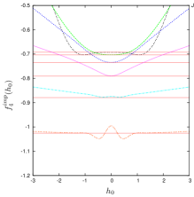
With the above points in mind, let us study the behavior of the improved functions in detail. Figure 1 exhibits the fourth-order improved free energy $f_{4}^{imp}$ as a function of $h_{0}$ for $J=0.01$, $0.1$, $0.2$, $0.3$, $0.4$, and $0.5$. As we vary $J$, there is a clear evolution of the shape of the improved free energy. This reflects the fact that there are two phases, corresponding to the small $J$ (disordered) phase and the large $J$ (ordered) phase in the Ising model. At small values of $J$ (i.e. in the high temperature region), the set of improved free energies form a clear plateau around $h_{0}=0$, at which the values of the improved free energies are good approximations of the exact value. This is not surprising, because the original free energy was obtained through a perturbative expansion in small $J$, and it already provides a good approximation of the exact value. As we have seen above, at $h_{0}=0$, which is on the plateau, the fourth-order improved free energy has the same form as the original.

Now, let us consider the case of relatively large $J$ (i.e. the low temperature region). In this case, it is seen that plateaux develop in the regions near $h_{0}\sim\pm 2$ as the order of the improved free energy increases. Thus, we can evaluate the approximate value of the free energy on these plateaux, which is found to be close to the exact value expressed by the horizontal line [Fig. 1]. We would like to emphasize that we have obtained the relatively large $J$ (ordered phase) physics from the data of small $J$ (disordered phase) expansions.

Figure 2: Dependences of the improved magnetizations $m^{imp}_{i}(h_{0})$ with respect to the auxiliary parameter $h_{0}$ at $J=0.1$.

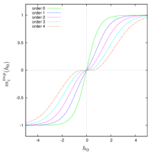
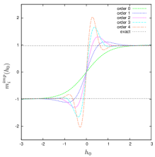
Although the emergence of plateaux at non-zero $h_{0}$ in the improved free energies may signal the occurrence of spontaneous magnetization, we have to investigate the magnetization itself to determine the amount by which the system magnetizes spontaneously. In Figs. 2 and 3, respectively, we plot the improved magnetizations from zeroth to fourth order for $J=0.1$ and $J=0.6$. In Fig. 2, it is seen that the slopes become gentle and a plateau emerges near the origin as the order increases. Contrastingly, Fig. 3 shows that the slopes at the origin become steeper as the order increases, whereas two plateaux develop near $h_{0}=\pm 2$. This figure also provides an approximate value of the magnetization that is close to the exact value, represented by the horizontal line in Fig. 3.

Figure 3: 3 Dependences of the improved magnetizations $m^{imp}_{i}(h_{0})$ with respect to the auxiliary parameter $h_{0}$ for $J=0.6$. 3 An enlarged plot near the exact value, which is represented by the horizontal line.

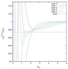
The two phases are characterized by spontaneous magnetization. If the plateau corresponds to the ground state realized at a particular value of $J$, the critical point can be recognized by the disappearance of the plateau formed at and near the origin. As mentioned above, the slope at the origin becomes steeper or gentler as we increase the order, depending on the value of $J$. Thus, at each order of approximation, the critical point is determined by the condition that the difference between the derivatives of the magnetizations at $n$th and $(n\!-\!1)$th orders be zero at the origin. Thus, we find

$$\left[\frac{\partial m^{imp}_{1}}{\partial h_{0}}-\frac{\partial m^{imp}_{0}}{\partial h_{0}}\right]_{h_{0}=0} =\quad 4J-1\,, \qquad(J_{c}^{(1)}=0.25)$$ (18a)

$$\left[\frac{\partial m^{imp}_{2}}{\partial h_{0}}-\frac{\partial m^{imp}_{1}}{\partial h_{0}}\right]_{h_{0}=0} =\quad 12J^{2}-4J\,, \qquad(J_{c}^{(2)}=0.33333)$$ (18b)

$$\left[\frac{\partial m^{imp}_{3}}{\partial h_{0}}-\frac{\partial m^{imp}_{2}}{\partial h_{0}}\right]_{h_{0}=0} =\quad\frac{104}{3}J^{3}-12J^{2}\,, \qquad(J_{c}^{(3)}=0.34615)$$ (18c)

$$\left[\frac{\partial m^{imp}_{4}}{\partial h_{0}}-\frac{\partial m^{imp}_{3}}{\partial h_{0}}\right]_{h_{0}=0} =\quad 92J^{4}-\frac{104}{3}J^{3}\,. \qquad(J_{c}^{(4)}=0.37681)$$ (18d)

It is seen that as we increase the order, the approximate value of the critical point moves closer to the exact value, $J_{c}=\frac{1}{2}\ln(1+\sqrt{2})=0.440\cdots$.

It is interesting that the quantity on the left-hand side of (18) is equal to the second derivative of the improved free energy with respect to $h_{0}$ at the origin:

$$\frac{\partial^{2}f^{imp}_{i}}{\partial h_{0}^{2}}\Bigg{|}_{h_{0}=0}=\left[\frac{\partial m^{imp}_{i}}{\partial h_{0}}-\frac{\partial m^{imp}_{i\!-\!1}}{\partial h_{0}}\right]_{h_{0}=0}\,.$$ (19)

Thus, the phase transition point can be understood in terms of the improved free energy in the following way. The plateau at the origin in the disordered phase is a local minimum, and as we increase $J$, it becomes a local maximum, and new minima appear. The critical point is the phase transition point.

It is also interesting to see what happens when we turn on an external magnetic field. For this purpose, we substitute $h=0.05$, as an example, in the improved functions.

Figure 4: 4 Dependences of the improved free energies $f^{imp}_{i}(h_{0})$ with respect to the auxiliary parameter $h_{0}$ in the case of a weak external field ($h=0.05$) and $J=0.6$. 4 An enlarged plot. The horizontal line represents the exact value in the case $h=0$.

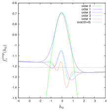
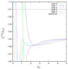
Turning on the external field causes the heights of two degenerate plateaux to become different [Fig. 4]. The plateau whose height increases corresponds to a metastable physical state (vacuum), and the other plateau corresponds to a stable physical state. Hence, the ITE reveals not only a stable vacuum but also a metastable one. However, as we increase the strength of the external field, the metastable plateau disappears, while the stable plateau retains its flat shape.

Strong field expansion.

Let us now proceed to the strong field expansion and construct a series in terms of $H=\exp(-2h)$:

$$Z(J,h)\equiv\sum_{n=0}^{\infty}H^{n}z_{n}(h)\,.$$ (20)

We calculate $z_{n}$ up to fourth order in $H$:

$$z_{0}(h) =e^{V(2J+h)},$$ (21a)

$$z_{1}(h) =z_{0}V\lambda^{2},$$ (21b)

$$z_{2}(h) =z_{0}V\left[2\lambda^{3}+\frac{1}{2}(V-5)\lambda^{4}\right],$$ (21c)

$$z_{3}(h) =z_{0}V\left[6\lambda^{4}+2(V-8)\lambda^{5}+\frac{1}{3!}\left(V^{2}-15V+62\right)\lambda^{6}\right],$$ (21d)

$$z_{4}(h) =z_{0}V\biggl{[}\lambda^{4}+18\lambda^{5}+(8V-85)\lambda^{6}+(V^{2}-21V+96)\lambda^{7}\biggr{.}$$

$$\qquad\left.+\frac{1}{4!}\left(V^{3}-30V^{2}+323V+714\right)\lambda^{8}\right],$$ (21e)

where $\lambda=\exp(-4J)$. The free energy density of $j$th order is defined as

$$f_{j}(J,h)=-\frac{1}{V}\ln\left(\sum_{n}H^{n}z_{n}(h)\right)\Bigg{|}_{j}.$$ (22)

We obtain the free energy of fourth order as

$$f_{4}(J,h) =-(2J+h)-\lambda^{2}H-\left(2\lambda^{3}-\frac{5}{2}\lambda^{4}\right)H^{2}-\left(6\lambda^{4}-16\lambda^{5}+\frac{31}{3}\lambda^{6}\right)H^{3}$$

$$\qquad-\left(\lambda^{4}+18\lambda^{5}-85\lambda^{6}+96\lambda^{7}-\frac{121}{4}\lambda^{8}\right)H^{4}\,,$$ (23)

and the magnetization as

$$m_{4}(J,h) =1-2\lambda^{2}H+4\left(-2\lambda^{3}+\frac{5}{2}\lambda^{4}\right)H^{2}+6\left(-6\lambda^{4}+16\lambda^{5}-\frac{31}{3}\lambda^{6}\right)H^{3}$$

$$\qquad-8\left(-\lambda^{4}-18\lambda^{5}+85\lambda^{6}-96\lambda^{7}+\frac{121}{4}\lambda^{8}\right)H^{4}\,.$$ (24)

In order to obtain improved functions, we make the substitutions

$$H \to gH\,,$$

$$\lambda \to\lambda_{0}+g(\lambda-\lambda_{0})$$ (25)

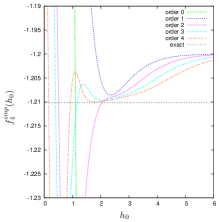
in the above expressions for the free energy and magnetization. Expanding about $g=0$ up to fourth order and setting $g=1$ at the end, we obtain the improved free energy $f^{imp}_{i}(H,J;\lambda_{0})$ and magnetization $m^{imp}_{i}(H,J;\lambda_{0})$. We set $H=1$ because we are interested in the case in which the external magnetic field is turned off. Here we present the fourth-order improved free energy $f^{imp}_{4}(H=1,J;\lambda_{0})$ and magnetization $m^{imp}_{4}(H=1,J;\lambda_{0})$ for various $J$ in Figs. 5 and 5.

Figure 5: 5 Dependences of the fourth-order improved free energies $f^{imp}_{4}(H=1,J;\lambda_{0})$. 5 Those of the improved magnetization $m^{imp}_{4}(H=1,J;\lambda_{0})$ in the strong field expansion for $J=0.3,0.4,0.5,0.6,\text{and\ }0.7$.

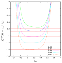
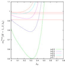
It is curious that there is no clear transition in the shape of the function as we vary the strength of $J$, in contrast to the previous case. Nonetheless, an indistinct signal can be seen that the plateau located near $\lambda_{0}=0$ moves to $\lambda_{0}>0$ below a certain value of $J$, which may imply the occurrence of a phase transition.

Conclusion.

We applied the improved Taylor expansion (ITE) to the Ising model in two dimensions and found that it is effective for extracting quantities in strong coupling regions from the weak coupling expansion, even though these two regions are separated by a phase transition. We obtained a good approximation for the observable in the ordered phase from a perturbation theory formulated in the disordered phase. We also determined approximate values of the critical point at each order of the approximation by closely examining improved functions of the magnetization, in particular at the origin of the auxiliary parameter space. Furthermore, turning on a small external field the ITE reveals the existence of not only a stable vacuum but also a metastable one. We also applied the ITE to the strong field expansion and found that it also works well for evaluating the free energy and magnetization in weak coupling regions, even though there is only a weak signal indicating the phase transition, which can be seen clearly in the weak coupling expansion.

We note that the ITE at first order is identical to the ordinary mean field approximation when we adopt a criterion for the identification of the plateau using the stationary points of the improved free energy. The condition that the derivative of the improved free energy with respect to the auxiliary parameter be zero should here play the role of the self-consistency condition in the mean field approximation. Extensions of the mean field approximation have been explored, e.g., in the Bethe approximation, in such a way that the quantum degrees of freedom of neighboring sites are taken into account step by step. This approach incorporates the higher order contributions successively, while the physical picture is apparent. Our ITE scheme also provides a systematic extension in a simple manner based on the variational method in a purely mathematical sense. It turns out, however, that the ITE is different from Bethe approximation already at second order, and the physical meaning of the extension is not obvious. It would be interesting to clarify the role of the plateau and its relation to the self-consistency condition in the mean field approximation. It would also be interesting to evaluate various critical exponents within the ITE scheme as a future work.

Appendix A Improved Functions

Here we list the improved free energy and magnetization up to fourth order in the weak coupling expansion. In the following, we employ the quantity $k_{0}\equiv\tanh(h_{0})$.

$$f^{imp}_{0}(J,h;h_{0})=-\ln(2\cosh(h_{0})),$$ (26a)

$$f^{imp}_{1}(J,h;h_{0})=-\{\ln(2\cosh(h_{0}))+k_{0}(h-h_{0})\}-2k_{0}^{2}J,$$ (26b)

$$f^{imp}_{2}(J,h;h_{0})=-\left\{\ln(2\cosh(h_{0}))+k_{0}(h-h_{0})+\frac{1}{2}(1-k_{0}^{2})(h-h_{0})^{2}\right\}$$

$$\qquad-\{(4k_{0}-4k_{0}^{3})(h-h_{0})+2k_{0}^{2}\}J-\{1+6k_{0}^{2}-7k_{0}^{4}\}J^{2},$$ (26c)

$$f^{imp}_{3}(J,h;h_{0})=-\left\{\ln(2\cosh(h_{0}))+k_{0}(h-h_{0})+\frac{1}{2}(1-k_{0}^{2})(h-h_{0})^{2}\right.$$

$$\qquad\left.-\frac{1}{3}(k_{0}-k_{0}^{3})(h-h_{0})^{3}\right\}-\{2k_{0}^{2}+(4k_{0}-4k_{0}^{3})(h-h_{0})$$

$$\qquad+(2-8k_{0}^{2}+6k_{0}^{4})(h-h_{0})^{2}\}J-\{1+6k_{0}^{2}-7k_{0}^{4}$$

$$\qquad+(12k_{0}-40k_{0}^{3}+28k_{0}^{5})(h-h_{0})\}J^{2}-\left\{\frac{52}{3}k_{0}^{2}-56k_{0}^{4}+\frac{116}{3}k_{0}^{6}\right\}J^{3},$$ (26d)

$$f^{imp}_{4}(J,h;h_{0})=-\left\{\ln(2\cosh(h_{0}))+k_{0}(h-h_{0})+\frac{1}{2}(1-k_{0}^{2})(h-h_{0})^{2}\right.$$

$$\qquad\left.-\frac{1}{3}(k_{0}-k_{0}^{3})(h-h_{0})^{3}+\left(-\frac{1}{12}+\frac{1}{3}k_{0}^{2}-\frac{1}{4}k_{0}^{4}\right)(h-h_{0})^{4}\right\}$$

$$\qquad-\biggl{\{}2k_{0}^{2}+(4k_{0}-4k_{0}^{3})(h-h_{0})+(2-8k_{0}^{2}+6k_{0}^{4})(h-h_{0})^{2}$$

$$\qquad\left.+\left(-\frac{16}{3}k_{0}+\frac{40}{3}k_{0}^{3}-8k_{0}^{5}\right)(h-h_{0})^{3}\right\}J-\{1+6k_{0}^{2}-7k_{0}^{4}$$

$$\qquad+(12k_{0}-40k_{0}^{3}+28k_{0}^{5})(h-h_{0})+(6-66k_{0}^{2}+130k_{0}^{4}-70k_{0}^{6})(h-h_{0})^{2}\}J^{2}$$

$$\qquad-\left\{\frac{52}{3}k_{0}^{2}-56k_{0}^{4}+\frac{116}{3}k_{0}^{6}+\left(\frac{104}{3}k_{0}-\frac{776}{3}k_{0}^{3}+456k_{0}^{5}-232k_{0}^{7}\right)(h-h_{0})\right\}J^{3}$$

$$\qquad-\left\{\frac{5}{6}+46k_{0}^{2}-\frac{937}{3}k_{0}^{4}+526k_{0}^{6}-\frac{521}{2}k_{0}^{8}\right\}J^{4},$$ (26e)

$$m^{imp}_{0}(J,h;h_{0})=k_{0},$$ (27a)

$$m^{imp}_{1}(J,h;h_{0})=\{k_{0}+(1-k_{0}^{2})(h-h_{0})\}+\{4k_{0}-4k_{0}^{3}\}J,$$ (27b)

$$m^{imp}_{2}(J,h;h_{0})=\{k_{0}+(1-k_{0}^{2})(h-h_{0})+(-k_{0}+k_{0}^{3})(h-h_{0})^{2}\}$$

$$\qquad+\{4k_{0}-4k_{0}^{3}+(4-16k_{0}^{2}+12k_{0}^{4})(h-h_{0})\}J+\{12k_{0}-40k_{0}^{3}+28k_{0}^{5}\}J^{2},$$ (27c)

$$m^{imp}_{3}(J,h;h_{0})=\biggl{\{}k_{0}+(1-k_{0}^{2})(h-h_{0})+(-k_{0}+k_{0}^{3})(h-h_{0})^{2}$$

$$\qquad\left.+\left(-\frac{1}{3}+\frac{4}{3}k_{0}^{2}-k_{0}^{4}\right)(h-h_{0})^{3}\right\}+\{4k_{0}-4k_{0}^{3}+(4-16k_{0}^{2}+12k_{0}^{4})(h-h_{0})$$

$$\qquad+(-16k_{0}+40k_{0}^{3}-24k_{0}^{5})(h-h_{0})^{2}\}J$$

$$\qquad+\{12k_{0}-40k_{0}^{3}+28k_{0}^{5}+(12-132k_{0}^{2}+260k_{0}^{4}-140k_{0}^{6})(h-h_{0})\}J^{2}$$

$$\qquad+\left\{\frac{104}{3}k_{0}-\frac{776}{3}k_{0}^{3}+456k_{0}^{5}-232k_{0}^{7}\right\}J^{3},$$ (27d)

$$m^{imp}_{4}(J,h;h_{0})=\biggl{\{}k_{0}+(1-k_{0}^{2})(h-h_{0})+(-k_{0}+k_{0}^{3})(h-h_{0})^{2}$$

$$\qquad\left.+\left(-\frac{1}{3}+\frac{4}{3}k_{0}^{2}-k_{0}^{4}\right)(h-h_{0})^{3}+\left(\frac{2}{3}k_{0}-\frac{5}{3}k_{0}^{3}+k_{0}^{5}\right)(h-h_{0})^{4}\right\}$$

$$\qquad+\biggl{\{}4k_{0}-4k_{0}^{3}+(4-16k_{0}^{2}+12k_{0}^{4})(h-h_{0})+(-16k_{0}+40k_{0}^{3}-24k_{0}^{5})(h-h_{0})^{2}$$

$$\qquad\left.+\left(-\frac{16}{3}+\frac{136}{3}k_{0}^{2}-80k_{0}^{4}+40k_{0}^{6}\right)(h-h_{0})^{3}\right\}J$$

$$\qquad+\{12k_{0}-40k_{0}^{3}+28k_{0}^{5}+(12-132k_{0}^{2}+260k_{0}^{4}-140k_{0}^{6})(h-h_{0})$$

$$\qquad+(-132k_{0}+652k_{0}^{3}-940k_{0}^{5}+420k_{0}^{7})(h-h_{0})^{2}\}J^{2}$$

$$\qquad+\left\{\frac{104}{3}k_{0}-\frac{776}{3}k_{0}^{3}+456k_{0}^{5}-232k_{0}^{7}\right.$$

$$\qquad\left.+\left(\frac{104}{3}-\frac{2432}{3}k_{0}^{2}+3056k_{0}^{4}-3904k_{0}^{6}+1624k_{0}^{8}\right)(h-h_{0})\right\}J^{3}$$

$$\qquad+\left\{92k_{0}-\frac{4024}{3}k_{0}^{3}+\frac{13216}{3}k_{0}^{5}-5240k_{0}^{7}+2084k_{0}^{9}\right\}J^{4}.$$ (27e)

References

- [1] V. I. Yukalov, Mosc. Univ. Phys. Bull. 31 (1976), 10.
- [2] P. M. Stevenson, Phys. Rev. D 23 (1981) 2916.
-
[3]
R. Guida, K. Konishi and H. Suzuki,
Annals Phys. 241 (1995) 152;
R. Guida, K. Konishi and H. Suzuki, Annals Phys. 249 (1996) 109. - [4] D. Kabat and G. Lifschytz, Nucl. Phys. B 571 (2000) 419.
[5]
S. Oda and F. Sugino,
JHEP 0103 (2001) 026;
F. Sugino, JHEP 0107 (2001) 014. - [6] J. Nishimura, T. Okubo and F. Sugino, JHEP 0210 (2002) 043.
- [7] J. Nishimura, T. Okubo and F. Sugino, JHEP 0310 (2003) 057.
- [8] J. Nishimura, T. Okubo and F. Sugino, Prog. Theor. Phys. 114 (2005) 487.
- [9] J. Nishimura and F. Sugino, JHEP 0205 (2002) 001.
- [10] H. Kawai, S. Kawamoto, T. Kuroki, T. Matsuo and S. Shinohara, Nucl. Phys. B 647 (2002) 153.
- [11] H. Kawai, S. Kawamoto, T. Kuroki and S. Shinohara, Prog. Theor. Phys. 109 (2003) 115.
- [12] T. Aoyama and H. Kawai, “Higher order terms of improved mean field approximation for IIB matrix model and emergence of four-dimensional space-time,” arXiv:hep-th/0603146.
- [13] S. Shinohara, “Improved Mean Field Approximation and Improved Taylor Expansion: approximation schemes to extract non-perturbative dynamics from IIB matrix model”, Kyoto University Ph.D. thesis (2003), in Japanese.
- [14] S. Kawamoto and T. Matsuo, “Improved renormalization group analysis for Yang-Mills theory,” arXiv:hep-th/0307171.
- [15] T. Aoyama and Y. Shibusa, “Improved Perturbation Method and its Application to the IIB Matrix Model,” arXiv:hep-th/0604211.
- [16] Phase Transitions and Critical Phenomena (Academic Press, London, 1974), Ed. C. Domb and M. S. Green.
- [17] L. Onsager, Phys. Rev. 65 (1944), 117.
[18]
L. Onsager, Nuovo Cim. Suppl. 6 (1949), 261.
C. N. Yang, Phys. Rev. 85 (1952), 808. - [19] G. Parisi, Statistical Field Theory, FRONTIERS IN PHYSICS, 66 (Addison-Wesley, 1988).