UT-05-14

NSF-KITP-05-79

hep-th/0510061

Distribution of Flux Vacua around
Singular Points in Calabi-Yau Moduli Space



Tohru Eguchi¹ and Yuji Tachikawa^1,2

¹ Department of Physics, Faculty of Science,
University of Tokyo, Tokyo 113-0033, JAPAN

² Kavli Institute for Theoretical Physics,
University of California, Santa Barbara, CA 93106 , USA

abstract

We study the distribution of type IIB flux vacua in the moduli space near various singular loci, e.g. conifolds, ADE singularities on ${\bf P}^{1}$, Argyres-Douglas point etc, using the Ashok-Douglas density $\det(R+\omega)$. We find that the vacuum density is integrable around each of them, irrespective of the type of the singularities. We study in detail an explicit example of an Argyres-Douglas point embedded in a compact Calabi-Yau manifold.

1 Introduction

Recently the problem of moduli stabilization and the landscape of flux vacua in string theory are receiving a great deal of attentions [1, 2, 3, 4] (for an earlier reference, see [5]). In the case of type IIB string theory, for instance, a non-zero superpotential is generated and complex structure moduli become fixed at its extremum when one introduces RR and NSNS 3-form fluxes passing through cycles of the Calabi-Yau (CY) manifold. Kähler moduli may also be fixed when CY manifold obeys a certain topological condition and D-brane instanton amplitudes become non-vanishing[3, 6, 7] . It turns out, however, that such a mechanism of moduli stabilization leads to an enormously large (possibly infinite) number of vacua in type IIB string theory. Problem of vacuum selection is now becoming one of the most challenging issues in superstring theory.

Actually the flux vacua are not distributed uniformly over the whole of moduli space of CY manifolds. Instead they are sharply peaked around the singular loci in the CY moduli space, such as the conifold points [11, 12]. It is well-known that various interesting non-perturbative phenomena take place at these singular points; i) appearance of massless matter at the conifold point[14], ii) generation of non-Abelian gauge symmetry at the ADE-singularities (fibered over ${\bf P}^{1}$) [15], iii) emergence of mutually non-local massless solitons and scale invariance at Argyres-Douglas point[16, 17, 18] etc. Thus it seems worthwhile to study in some detail the behavior of flux vacua around the singular loci of CY moduli space.

In this paper we will use the density formula $\det(R+\omega)$ of Ashok and Douglas [11] ($R$ and $\omega$ denotes the curvature and the Kähler form of the moduli space) for the flux vacua in the type IIB string theory and estimate the behavior of vacuum density near Calabi-Yau singularities. We shall show that the following behavior

$$\mbox{vacuum density}\approx\frac{dz\,d\bar{z}}{|z|^{2}(\log|z|)^{p}},\qquad p:\mbox{positive integer, $p\geq 2$}$$ (1.1)

holds universally irrespective of the nature of singularities (conifolds, $\mathbf{P}^{1}$ fibration of ADE singularities, Argyres-Douglas point etc.) with the value of integer $p$ depending on the specific cases. Here $z$ denotes a coordinate in moduli space with the singularity located at $z=0$. The above formula has been known in the case of conifold singularity, and it is also verified numerically in some cases [19, 20].

We note that the vacuum density is in fact normalizable

$$\int\mbox{vacuum density}<\infty,$$ (1.2)

which roughly states that there exist only a finite number of vacua concentrated around each singular locus. This seems to be a further result suggesting the finiteness of the number of vacua in the type IIB string landscape (see a very recent discussion in [21]).

The structure of the paper is as follows: in section 2, we review the Ashok-Douglas formula and necessary ingredients. The discussion will be brief and is mainly to fix the convention. In section 3, we lay out the basic strategies of studying the growth of the Ashok-Douglas density near the singular locus in the moduli space. The actual analysis is done in section 4. In section 5, we take a specific Calabi-Yau to examine a concrete example, and study the geometric-engineering limit and the Argyres-Douglas points. We conclude in section 6 with some discussion.

Note Added: During the preparation of the manuscript, we have noticed a very short announcement in the mathematics archive [22] where results related to ours are discussed.

2 Preliminaries

In this section we introduce our notations and conventions and review the Ashok-Douglas formula.

2.1 Kähler geometry

We denote by $K$ the Kähler potential of the manifold. In supergravity, the Kähler manifold of the sigma model target space needs to be a Hodge manifold, that is, its Kähler form must be equal to the curvature of some holomorphic line bundle $L$ in the Planck units[23]. A holomorphic section $s$ of the bundle $L^{\otimes p}$ transforms as $s\to e^{pf}\,s$ under the Kähler transformation $K\to K+f+\bar{f}$. The superpotential of a supergravity theory is a holomorphic section of $L^{-1}$. The covariant derivatives for the section of $L^{\otimes p}$ are given by

$$D_{i}=\partial_{i}-p(\partial_{i}K),$$ (2.1)

$$\bar{D}_{\bar{i}}=\bar{\partial}_{\bar{i}}.$$ (2.2)

Here $\partial_{i}=\partial/\partial z_{i}$ and $z_{i}$ denotes the coordinates on the manifold. If one considers in general a Hermitean vector bundle $E$ with a connection $A=A_{i}dz^{i}$ ($A_{i}=-p\,\partial_{i}K$ in (2.1)), the curvature form is defined as

$$F=(dz^{i}D_{i}+d\bar{z}^{\bar{i}}\bar{D}_{\bar{i}})^{2}=\bar{\partial}A.$$ (2.3)

The metric $g_{i\bar{j}}$ of a Kähler manifold is given by $\partial_{i}\partial_{\bar{j}}K$ and the Kähler form is defined by

$$\omega=idz^{i}\wedge d\bar{z}^{\bar{j}}g_{i\bar{j}}=i\partial\bar{\partial}K.$$ (2.4)

Then, the first Chern class of $L^{\otimes p}$ is given by

$$c_{1}(L^{\otimes p})=\frac{-ip}{2\pi}\bar{\partial}\partial K=\frac{p\,\omega}{2\pi}.$$ (2.5)

For the holomorphic tangent bundle, the connection one-form is

$$A=g^{i\bar{k}}\partial g_{j\bar{k}}$$ (2.6)

Components of the Riemann tensor are given by

$$R_{i\bar{j}k\bar{l}}=g_{n\bar{l}}\,\partial_{\bar{j}}g^{n\bar{m}}\partial_{k}g_{i\bar{m}}.$$ (2.7)

Curvature two-form is then written as

$$R=ig^{m\bar{l}}R_{i\bar{j}k\bar{l}}\,d\bar{z}^{\bar{j}}\wedge dz^{k}.$$ (2.8)

Thus the top Chern class of the bundle $L^{-1}\otimes\Omega^{(1,0)}{\cal M}$ is

$$\det(-\frac{R}{2\pi}-\frac{\omega}{2\pi}).$$ (2.9)

When the bundle is positive, it calculates the number of zeros of its generic section.

2.2 Special Kähler geometry

Compactification of Type IIB string on Calabi-Yau with fluxes inherits certain properties from compactification without flux. Thus, part of the structure of the $\mathcal{N}=2$ supergravity in four dimension comes into play. Let us recall the structure of the vector multiplet scalars in the $\mathcal{N}=2$ supergravity. We denote the number of the vector multiplets by $n$.

Let $n$ complex scalars $z_{i}$, $i=1,\ldots,n$ parametrize the scalar manifold $\mathcal{M}$. Fundamental data defining the special Kähler geometry is the flat vector bundle $V$ of rank $2n+2$ equipped with the symplectic pairing $\eta^{IJ},\,I,J=1,2,\ldots,2n+2$ and the holomorphic section $\Omega=\{\Omega_{I}\}$ of the bundle $L^{-1}\otimes V$. $\Omega_{I}$ are called as the periods, or the (projective) special coordinates of the manifolds. We sometimes abbreviate the pairing $\eta^{IJ}A_{I}B_{J}$ of two vectors as $\eta AB$ if no confusion would arise.

The periods are constrained by the transversality condition

$$\eta^{IJ}\Omega_{I}\partial_{i}\Omega_{J}=0.$$ (2.10)

One can recover the prepotential $F$ in the following way: Introduce another variable $z_{0}$ parametrizing $\mathbb{C}$ and consider a manifold $\mathbb{C}\times\mathcal{M}$. Define functions $\Omega_{I}(z_{0},z)$ on $\mathbb{C}\times\mathcal{M}$ by $\Omega_{I}(z_{0},z)=z_{0}\Omega_{I}(z)$. Let us note that eq. (2.10) holds also on $\mathbb{C}\times\mathcal{M}$, including $\partial_{i}=\partial_{z_{0}}$. We take a canonical symplectic basis and split $\Omega_{I}$ into $(X^{\Lambda},F_{\Lambda})$ ($\Lambda$ runs from $0$ to $n$). We introduce a function $F$ by the formula $F=X^{\Lambda}F_{\Lambda}/2$. $\mathbb{C}\times\mathcal{M}$ can be parametrized by $X^{0},\ldots,X^{N}$. Then (2.10) in this coordinate system reads

$$F_{\Sigma}\partial_{\Lambda}X^{\Sigma}-X^{\Sigma}\partial_{\Lambda}F_{\Sigma}=0,\qquad\text{i.e.}\quad F_{\Lambda}=X^{\Sigma}\partial_{\Lambda}F_{\Sigma}.$$ (2.11)

Thus we have

$$\frac{\partial F}{\partial X^{\Lambda}}=\frac{F_{\Lambda}}{2}+\frac{1}{2}X^{\Sigma}\partial_{\Lambda}F_{\Sigma}=F_{\Lambda}.$$ (2.12)

Standard formulae of special geometry[24, 25] are then given by

$$K =-\log i\eta^{IJ}\bar{\Omega}_{I}\Omega_{J},$$ (2.13)

$$e^{K} =1/(i\eta\bar{\Omega}\Omega),$$ (2.14)

$$g_{i\bar{j}} =-\frac{\eta\partial_{\bar{j}}\bar{\Omega}\partial_{i}\Omega}{(\eta\bar{\Omega}\Omega)}+\frac{(\eta\bar{\Omega}\partial_{i}\Omega)(\eta\bar{\partial}_{\bar{j}}\bar{\Omega}\Omega)}{(\eta\bar{\Omega}\Omega)^{2}},$$ (2.15)

$$F_{ijk} =\eta^{IJ}\Omega_{I}\partial_{i}\partial_{j}\partial_{k}\Omega_{J}=-\eta^{IJ}\partial_{i}\Omega_{I}\partial_{j}\partial_{k}\Omega_{J},$$ (2.16)

$$R_{i\bar{j}k\bar{l}} =g_{i\bar{j}}g_{k\bar{l}}+g_{i\bar{l}}g_{k\bar{j}}-e^{2K}g^{m\bar{n}}F_{ikm}\bar{F}_{\bar{j}\bar{l}\bar{n}}.$$ (2.17)

Note that the $\Omega_{I}$ may be multivalued because of the holonomy or monodromy of $V$ in $\mathop{\mathrm{Sp}}(2n+2,\mathbb{Z})$. $F_{ijk}$ and $R_{i\bar{j}k\bar{l}}$ are invariant under the monodromy transformation.

2.3 Flux superpotential and Landscape

The space of complex structure moduli $\mathcal{M}$ of a CY threefold $X$ is a special Kähler manifold of complex dimension $n=h^{1,2}(X)$. The periods $\Omega_{I}$ are given by

$$\Omega_{I}=\int_{C_{I}}\Omega(z_{i})$$ (2.18)

where $C_{I}$ is a basis of three-cycles in $X$ and $\Omega$ is the holomorphic three-form of $X$. $\Omega$ depends on the moduli of the Calabi-Yau manifold. The fact $\Omega$ is defined only up to the scalar multiple depending on the moduli is reflected to the fact that the Kähler transformation acts on $\Omega_{I}$.

Let us compactify type IIB theory on $X$. When one introduces NSNS and RR fluxes $H^{NSNS},H^{RR}$, one obtains a four-dimensional $\mathcal{N}=1$ supergravity theory with a superpotential

$$W=\eta^{IJ}(\tau H^{NSNS}_{I}+H^{RR}_{I})\Omega_{J},$$ (2.19)

where $\tau$ is the axiodilaton and $H^{NSNS}_{I},H^{RR}_{I}$ are the integral fluxes passing through the three-cycles $C_{I}$ [26, 27].

The flux superpotential (2.19) generically gives masses to the complex structure moduli and the axiodilaton. One needs to introduce a certain number of D3 branes and orientifolding in order to satisfy the tadpole cancellation condition, which in general puts restrictions on the allowed values of the fluxes.

There are also the moduli for the Kähler deformation in CY manifolds and for the complete moduli stabilization we also have to consider mechanisms to give masses to the Kähler moduli. In this paper we restrict our attention to the sector of complex moduli of CY manifolds.

A number of choices is possible for the set of integer fluxes $H^{NSNS}_{I},H^{RR}_{I},\,I=1,\ldots,2n+2$ and this is the origin of the existence of enormous number of flux vacua in type IIB theory. We may study the statistical distribution of these vacua in the moduli space[4, 11], instead of studying them one by one. We do not know the dynamical mechanism behind the a priori probability distribution of the fluxes $H_{I}^{NSNS},H_{I}^{RR}$. A zero-th order approximation may be to assume that the fluxes obey a Gaussian distribution. Then, the correlators among the superpotential at various points on the moduli are given by

$$\langle W(z_{i})W^{*}(w_{i})\rangle \propto e^{-K(z_{i},w_{i}^{*})},$$ (2.20)

$$\langle W(z_{i})W(w_{i})\rangle =0=\langle W^{*}(z_{i})W^{*}(w_{i})\rangle.$$ (2.21)

From the point of view of the study of the distribution of vacua under random superpotentials, we may concentrate on what can be derived from the basic correlation functions (2.20) and (2.21).

Supersymmetric AdS vacua are at the extrema of the superpotential, $D_{i}W=0$. The distribution function of such vacua over the moduli space is given by

$$\rho(z,\bar{z})=\langle\delta(D_{i}W(z))\delta(\bar{D}_{\bar{\imath}}W(\bar{z})^{*})\left|\det\begin{pmatrix}\partial_{i}D_{j}W&\partial_{i}D_{\bar{\jmath}}W^{*}\\ \partial_{\bar{\imath}}D_{j}W&\partial_{\bar{\imath}}D_{\bar{j}}W^{*}\end{pmatrix}\right|\rangle.$$ (2.22)

The absolute value is required to count each vacua with a weight one. It is somewhat difficult to evaluate this quantity because of the absolute value sign. We may consider instead

$$\tilde{\rho}(z,\bar{z})=\langle\delta(D_{i}W(z))\delta(\bar{D}_{\bar{\imath}}W(\bar{z})^{*})\det\begin{pmatrix}\partial_{i}D_{j}W&\partial_{i}D_{\bar{\jmath}}W^{*}\\ \partial_{\bar{\imath}}D_{j}W&\partial_{\bar{\imath}}D_{\bar{j}}W^{*}\end{pmatrix}\rangle$$ (2.23)

which counts vacua with a sign. Ashok and Douglas showed in [11] that it is given by

$$\tilde{\rho}(z,\bar{z})\prod_{i}dz^{i}\wedge d\bar{z}^{\bar{\imath}}\propto\det(-\frac{R^{i}{}_{j}}{2\pi}-\frac{\delta^{i}{}_{j}\omega}{2\pi}).$$ (2.24)

The right hand side is the determinant of the curvature tensor of $\Omega^{(1,0)}{\cal M}\otimes L^{-1}$, of which $D_{i}W$ is the section. Since $\tilde{\rho}$ gives the lower bound for the number of vacua $\rho$, the formula tells that the vacua do not distribute uniformly. Rather, they tend to concentrate near the points where the curvature of the moduli space is peaked. Thus, it is of importance to study the convergence property of (2.24) near various kind of singularities in the moduli space, which is the main objective of our study.

3 Strategy of the analysis

In the following, we study the behavior of the Ashok-Douglas density (2.24) on the complex structure moduli space alone, neglecting the contribution from the axiodilaton and other scalar fields. This is not going to be the full answer to our problem, but is hopefully an important step in that direction.

Before proceeding, we would like to mention the relation of our work with those in the mathematical literature. When phrased in purely mathematical terms, our work studies the convergence properties of various products of Chern classes and Kähler forms near the singular loci of the CY moduli space. If one chooses the $n$-th power of the Kähler forms as the integrand, the problem becomes precisely the convergence of the volume of the moduli space of Calabi-Yau studied in [28, 29]. The integral of the products of the first Chern class and the Kähler form was studied in [30] and was shown to be finite. What we need to study is basically the sum of all possible Chern classes. In [31, 32], the distance to the singular locus was studied using a similar method.

3.1 Singularities in Calabi-Yau moduli space

As briefly reviewed in section 2.3, the moduli space $\mathcal{M}$ for the complex structure deformation of Calabi-Yau three-fold $X$ is a special Kähler manifold. It is not smooth and compact, however. It contains a number of so-called discriminant loci, around which the periods $\Omega_{I}$ have non-trivial monodromies preserving the symplectic pairing $\eta$. Each point on the complement of the discriminant loci corresponds to the non-singular Calabi-Yau. An important fact is that a deep mathematical theorem by Viehweg[33] ensures that the moduli space $\mathcal{M}$ of smooth Calabi-Yau manifolds $X$ is quasi-projective, that is, it can be realized as $\overline{\mathcal{M}}\setminus D$ where $\overline{\mathcal{M}}$ is a subvariety of some projective space and $D$ is a divisor. Although some kind of singular Calabi-Yau manifolds should correspond to the point of $D$, it is not known in complete generality which kind of singular Calabi-Yaus to allow in order to compactify $\mathcal{M}$ to $\overline{\mathcal{M}}$.

Components of $D$ intersect among themselves, and they in general develop singularities on them. For example, it is known that the Argyres-Douglas point corresponds to a cusp of the discriminant locus, as we will review below.

What greatly facilitates the analysis is that, using Hironaka’s theorem, we can resolve the singularity of $D$ by a number of blow-ups so that the singular loci $D$ can be made to have ‘normal crossings’, i.e. they intersect transversally. Thus, we can always take, near the intersection of $k$ singular loci, a coordinate patch of the form $(z_{1},\ldots,z_{n})\in(\Delta^{*})^{k}\times\Delta^{n-k}$ where $\Delta$ is a unit disk and $\Delta^{*}=\Delta\setminus 0$ is a punctured disk so that the loci themselves are given by $z_{1}z_{2}\cdots z_{k}=0$.

In understanding the divergence or the convergence of the curvature and the volume form near the discriminant loci, what we actually examine is the outside of the singular locus; thus the construction above can be seen as providing a good coordinate system to study the singular loci. For concrete examples of discriminant loci, we can indeed show in each case that the loci can be made to have normal crossings by an appropriate blow up procedure.

3.2 Monodromy and Schmid’s nilpotent orbit theorem

We are going to study the curvature of the moduli space. As a special Kähler manifold, all the properties are encoded in the behavior of the periods $\Omega_{I}$. Thus we first need a good control over the behaviors of $\Omega_{I}$ near the discriminant locus. As the periods are holomorphic, their properties are basically determined by the monodromies around the discriminant locus. We can study case by case how each monodromy type is related to a particular behavior of the curvature of moduli space. In the mathematical literature, however, a great deal is known on the generic properties of the monodromy matrix and the behavior of the periods.

The proper mathematical language to use is the pure and mixed Hodge structures. Although they are somewhat unwieldy, results from these subjects are essential. We have collected necessary definitions and the facts in the appendix A to fill the gap between language used in mathematics and in string theory. We present below the necessary results we use in the main part of the paper.

First, let us recall some terminologies. A matrix $N$ is called nilpotent when there is some integer $k$ such that $N^{k}=0$. A matrix $M$ is called unipotent when $M-1$ is nilpotent. A matrix $M$ is called quasi-unipotent if there is some integer $k$ such that $M^{k}$ is unipotent.

Traversing the circle around a singular locus leads to some automorphism $\gamma$ of the $H^{3}(X,\mathbb{Z})$ which preserves the intersection form. We call $\gamma$ the monodromy matrix. It is known that $\gamma$ is quasi-unipotent. Thus there exists some integer $k$ and some nilpotent matrix $N$ such that $\gamma^{k}=\exp(N)$. $N$ is known to satisfy $N^{4}=0$. The sketch of the proof is provided in the appendix A.3.

Let us introduce a coordinate $z$ such that $z=0$ is the singular locus. The nilpotent orbit theorem of Schmid says that (precise statement is reproduced in the appendix A.2)

$$\Omega^{\prime}\equiv\exp(-\frac{N}{2\pi ik}\log z)\Omega,\hskip 11.38109pt(\Omega\mbox{ is a column vector made of periods }\Omega_{I})$$ (3.1)

is analytic in $z^{1/k}$ in a suitable Kähler gauge and starts with a nonzero constant term. That is, there appear no negative powers of $z$ in the periods $\Omega^{\prime}$. Taking the coordinate change $z^{1/k}\to z$, we can assume that there appear no fractional powers without losing generality.

Let us suppose that a singular locus lies at $z=0$, and expand the periods using the nilpotent orbit theorem as

$$\Omega_{I}=\sum_{i,j\geq 0}c_{Iij}z^{i}(\log z)^{j}.$$ (3.2)

We will see that whether nonzero $c_{I,0,j}$ with $j>0$ exists or not affects the behavior of various quantities via the divergence or convergence of $e^{-K}$ at $z=0$. Hence we will split the following discussions to two cases. Case I is when all $c_{I,0,j}$ is zero for $j>0$; Case II is when some of $c_{I,0,j}$ is nonzero $j>0$. As we will see in the following, conifold singularities and Argyres-Douglas singularities are included in Case I , while the large complex structure and the geometric engineering limit are included in Case II. Case I is treated in section 4.1 and Case II is treated in section 4.2.

4 Generic Estimate of the Growth

After these preparations, we study the growth of the Ashok-Douglas density $\det(R+\omega)$ near the singularity. First, note that

$$\text{index density}\approx dzd\bar{z}\sqrt{g}\epsilon^{\overbrace{.......}^{2n}}\epsilon^{\overbrace{........}^{2n}}\overbrace{Q_{....}Q_{.....}\cdots Q_{.....}}^{n}$$ (4.1)

where $Q_{....}$ is a linear combination of $e^{2K}F_{...}\bar{F}_{...}g^{..}$ and $g_{..}g_{..}$. The dots denote various indices to be contracted.

Next, we rewrite $\epsilon^{....}\epsilon^{.....}$ by a totally-antisymmetrized product of $2n$ inverse metrics $g^{[.[.}g^{..}g^{..}\cdots g^{.].]}$. Furthermore, we express $Q$ as a contraction of $g^{..}$ with a linear combination of $e^{2K}F_{...}\bar{F}_{...}$ and $g_{..}g_{..}g_{..}$. Then the density is written schematically as

$$\propto dzd\bar{z}\sqrt{g}\underbrace{\overbrace{g^{..}g^{..}\cdots g^{..}}^{3n}\overbrace{(e^{2K}F_{...}\bar{F}_{...}+g_{..}g_{..}g_{..})\cdots(e^{2K}F_{...}\bar{F}_{...}+g_{..}g_{..}g_{..})}^{n}}_{\text{denote this part by $I$}}$$ (4.2)

We expand the factor $I$ and rewrite it as a sum of terms of the form $g^{..}\cdots g^{..}e^{2mK}F_{...}\bar{F}_{...}\\ \cdots F_{...}\bar{F}_{...}g_{..}\cdots g_{..}$. By contracting $g_{..}$ with $g^{..}$, each term in $I$ is reduced to the form

$$g^{..}\cdots g^{..}e^{2mK}F_{...}\bar{F}_{...}\cdots F_{...}\bar{F}_{...}$$ (4.3)

without $g_{..}$ factors. Here $m$ is the number of times the factors $F\bar{F}$ are taken in the expansion. Thus, we need to estimate the growth of $e^{K}$, $F_{...}$ and $g^{..}$ and then to plug the result into (4.3).

4.1 Conifold

The symplectic pairing of $2n$ periods $\eta_{2n}$ splits into $\eta_{2}\oplus\eta_{2n-2}$, and we assume a monodromy acting on the periods $\Omega_{1},\Omega_{2},\ldots,$ to be of the form

$$\begin{pmatrix}1&m\\ 0&1\end{pmatrix}\oplus\mathrm{id}_{2n-2}$$ (4.4)

This is the familiar case of the conifold singularity. $m$ is given by the number and the charges of the multiplets which become massless at the singularity.

We take one of the special coordinates $a\equiv\Omega_{2}$ as a local coordinate and assume that the locus is given by $a=0$. Then, from the monodromy we deduce

$$\Omega_{1} \approx\frac{m}{2\pi i}a\log a+\cdots,$$ (4.5)

$$\Omega_{2} \equiv a,$$ (4.6)

$$\Omega_{3} \approx\cdots,$$ (4.7)

$$\vdots$$ (4.8)

where $\cdots$ denote analytic functions of $a$. There will be dependence on other coordinates, but it must all be analytic. We will call this kind of behavior of the periods as the conifold-type. This is case I in the classification given in the last section. An important point is that the Yukawa coupling $F_{ijk}$ is monodromy invariant, thus it should contain no $\log a$ factors.

To facilitate the calculation we switch to a variable $t$ defined by $a=e^{-t}$ and the problem is to find the divergence of various quantities near $\mathop{\mathrm{Re}}t\approx+\infty$. We denote the real and the imaginary part of $t$ by $r$ and $\theta$, respectively. $t$ and $t+2\pi i$ should be identified. Then the period behaves as

$$\Omega_{1} \approx-\frac{m}{2\pi i}te^{-t}+\cdots,$$ (4.9)

$$\Omega_{2} \equiv e^{-t},$$ (4.10)

$$\Omega_{3} \approx\cdots,$$ (4.11)

$$\vdots$$ (4.12)

Now the dots signify Taylor series in $e^{-t}$.

A fundamental result that the mixed Hodge structure on the singularity is polarized guarantees that $\eta\bar{\Omega}\Omega$ approaches a nonzero constant at $r\equiv\mathop{\mathrm{Re}}t\to\infty$. This means that there are some periods $\Omega_{3},\Omega_{4},\ldots$ which remains nonzero in the limit $a\to 0$. For further details, see appendix A.2.

Let us estimate various quantities around the conifold locus. We introduce letters $u,v,...$ to represent the coordinates other than $t$. Indices $i,j...$ label, as before, the generic coordinates of the moduli space.

Estimate of $g_{i\bar{j}}$

• Using the expansion above and the fact that $K$ is monodromy invariant, $K$ has expansions like

  $$\sum_{k=0}^{1}\sum_{l,m\geq 0}c_{k,l,m}(t+\bar{t})^{k}e^{-lt}e^{-m\bar{t}}.$$ (4.13)

  From the assumption, $c_{k,0,0}=0$ for $k>0$. On the other hand it is known that $c_{0,0,0}\neq 0$ from the theory of variation of Hodge structure, see appendix A.2. Thus $e^{K}$ has a nonzero limit when $r\to\infty$.

• Hence we find

  $$g_{t\bar{t}}\sim r^{p}e^{-2r},\qquad g_{t\bar{v}}\sim e^{-r},\qquad g_{u\bar{v}}\sim 1$$ (4.14)

  with $p=1$. We have introduced an integer $p$ so that it facilitates the generalization later.

• Thus $dtd\bar{t}\sqrt{g}\sim r^{p}e^{-2r}drd\theta$, which readily converges at $r\approx\infty$.

Estimate of $g^{i\bar{j}}$

• Break $g_{i\bar{j}}$ into two parts:

  $$g_{ij}=g_{ij}^{(0)}+\delta g_{ij}$$ (4.15)

  where $g^{(0)}$ contains $g_{t\bar{t}}$ and $g_{u\bar{v}}$, $\delta g$ contains $g_{t\bar{v}}$.

• Using the formula

  $$g^{-1}=g_{(0)}^{-1}-g_{(0)}^{-1}\delta gg_{(0)}^{-1}+\cdots,$$ (4.16)

  we find

  $$g^{t\bar{t}}\sim r^{-p}e^{2r},\qquad g^{t\bar{v}}\sim r^{-p}e^{r},\qquad g^{u\bar{v}}\sim 1.$$ (4.17)

Estimate of $F_{ijk}$

• $\partial_{t}\Omega_{I}$ at most behaves as $te^{-t}$ and is exponentially small.

• $\partial_{u}\Omega_{I}$ will be at most constant.

• Second-derivatives of $\Omega_{I}$ are exponentially small when they contain derivatives in $t$ and at most constant when do not.

• $F_{ijk}=\eta^{IJ}\partial_{i}\Omega_{I}\partial_{j}\partial_{k}\Omega_{J}$. Hence $F\sim e^{-t}$ if only one of $i,j,k$ is $t$, $F\sim e^{-2t}$ if two or three indices are $t$, and $F\sim 1$ otherwise. There is no prefactor of $t$ because $F$ is monodromy invariant.

Estimate of index density

• Recall the expansion (4.3) and let us plug in the estimate obtained so far. Let us notice that to each subscript $t$ or $\bar{t}$ there is a corresponding factor $e^{-r}$ (4.14), and to each superscript $t$ or $\bar{t}$ a factor $e^{r}$ (4.17), except for $F_{ttt}$ and its conjugate (they behave as $e^{-2r}$). Then, the summand in $I$ carries one positive power of exponential $e^{r}$ if it contains one $F_{ttt}$ (or its conjugate), and two positive powers of exponential $e^{2r}$ if it contains both $F_{ttt}$ and $\bar{F}_{\bar{t}\bar{t}\bar{t}}$. Hence the leading contribution to $dtd\bar{t}\sqrt{g}I$ are the terms containing $F_{ttt}$ and $\bar{F}_{\bar{t}\bar{t}\bar{t}}$. If we recall the behavior of the volume factor $dtd\bar{t}\sqrt{g}\approx drd\theta r^{p}e^{-2r}$, we find that the exponential factors altogether cancel in the index density.

• Finally let us show that the terms identified above contain a sufficiently large number of negative powers of $r$. The structure of the term is

  $$dtd\bar{t}\sqrt{g}F_{ttt}\bar{F}_{\bar{t}\bar{t}\bar{t}}F_{...}\bar{F}_{...}\cdots F_{...}\bar{F}_{...}g^{..}\cdots g^{..}.$$ (4.18)

  It turns out that the $F_{...}\,(\bar{F}_{...})$ appearing in (4.18) other than $F_{ttt}$ and $\bar{F}_{\bar{t}\bar{t}\bar{t}}$ carries at most one $t\,(\bar{t})$ in the subscript, because of the two epsilon symbols in (4.1)

  The more we use $g^{t\bar{t}}$ in contracting indices, the less suppression factors of $r^{-p}$ we have (4.17). Here there exist at least six $t$ and $\bar{t}$’s from $F_{ttt}\bar{F}_{\bar{t}\bar{t}\bar{t}}$, which guarantees the existence of at least a factor of $r^{-3p}$. By multiplying with $dtd\bar{t}\sqrt{g}$, we obtain

  $$\text{integrand}\approx drd\theta r^{-2p}$$ (4.19)

  which converges at $r=\infty$. Q.E.D.

An easy generalization is possible when the periods contains the terms of the form

$$\sim a^{k}(\log a)^{m}=e^{-kt}t^{m}$$ (4.20)

but there are no ‘bare’ $t=-\log a$ factors without being accompanied by powers of $a=e^{-t}$. We call these type of degeneration as the ‘generalized conifold-type’.

$e^{K}$ can be expanded again in the form

$$\sum_{k,l,m\geq 0}c_{k,l,m}(t+\bar{t})^{k}e^{-lt}e^{-m\bar{t}}.$$ (4.21)

Another condition is that $e^{K}$ is the sum of the products of periods and their conjugates, which does not contain bare factors of $t$. Thus when $c_{klm}$ is nonzero for $k>0$, $l$ and $m$ must be strictly positive. There is a maximum for $k$ for which $c_{k,l,m}$ is nonzero; we denote it by $p$. Then

$$g_{t\bar{t}}\sim r^{p}e^{-2r},\qquad g_{t\bar{v}}\lesssim e^{-r}$$ (4.22)

and the rest of the analysis above goes through unmodified. We can also show that the integral of vacuum density converges when two or more discriminant loci of generalized-conifold type intersect.

4.2 Large complex structure limit

Next we deal with the case where the periods have a bare $t=-\log a$ factor unaccompanied by $e^{-t}$ around the discriminant loci. Let us expand again the periods using the nilpotent orbit theorem,

$$\Omega_{I}=\exp(t\frac{N}{2\pi i})(\Omega_{I}^{(0)}+\Omega_{I}^{(1)}a+\Omega_{I}^{(2)}a^{2}+\cdots).$$ (4.23)

Let $p$ be the maximum integer such that $N^{p}\Omega_{I}^{(0)}\neq 0$ for some $I$. $i\eta\bar{\Omega}\Omega$ starts with the expansion

$$i\eta\bar{\Omega}\Omega=\sum_{k}c_{k}(t+\bar{t})^{k}+\text{exponentially small terms in $t$...}$$ (4.24)

A basic result of the variation of Hodge structure is that $c_{k}$ is zero for $k>p$ and nonzero for $k=p$ (see appendix A.2). It is also known that $p\leq 3$. Then $K\sim p\log(t+\bar{t})$. Thus

$$g_{t\bar{t}}\sim 1/r^{2},\qquad g_{t\bar{v}}\sim 1/r$$ (4.25)

These estimates guarantee the convergence of the volume. The inverse metric is

$$g^{t\bar{t}}\sim r^{2},\qquad g^{t\bar{v}}\sim r.$$ (4.26)

The rest of the discussion need to be done separately for $p=3$, $p=2$ and $p=1$.

• $p=1$. Then $F_{ttt}=\eta^{IJ}\Omega_{I}(\partial_{t})^{3}\Omega_{J}$ and $F_{ttu}=\eta^{IJ}\Omega_{I}(\partial_{t})^{2}\partial_{u}\Omega_{J}$ are exponentially small, because the derivatives with respect to $t$ kill the $O(t)$ and $O(1)$ factors. Thus, the term which is not exponentially small contains only $F_{tuv}$ type terms. Hence the number of the subscript $t$ to be contracted is at most equal to the number of $F$. As each $F$ is accompanied by $e^{K}\sim 1/r$, this cancels the positive factors of $r$ from the inverse metric. Thus $I$ is bounded from above by a constant.

• $p=2$. Just as in the previous case, one finds $F_{ttt}$ to be exponentially small. Thus, in the terms which are not exponentially small, the number of the subscript $t$ to be contracted by $g^{t\bar{t}}$ or $g^{t\bar{v}}$ is at most equal to twice the number of $F$. This means the term is convergent, since each $F$ is accompanied by a factor $e^{K}\sim 1/r^{2}$.

• $p=3$. $F_{ijk}$ is at most constant as they are monodromy invariant and each is accompanied by a factor of $e^{K}\sim 1/r^{3}$. Thus the convergence of the index density is guaranteed.

4.3 Landau-Ginzburg point

Lastly, we would like to discuss the behavior of the vacuum index density around the Landau-Ginzburg (LG) point for completeness. In the case of quintic hypersurfaces, the monodromy $M$ satisfies $M^{5}=1$ at the LG point, that is , the monodromy is idempotent. Here we call any singular loci with idempotent monodromy LG-type loci.

Suppose we have a singular locus with monodromy matrix $M$ which satisfies $M^{p}=1$. Let the singular locus lie at $a=0$ with $a$ as the local coordinate of the disk. Changing variables to $z$ with the relation $a=z^{p}$, we obtain a variation of Calabi-Yau manifolds with trivial monodromy. From the nilpotent orbit theorem, the periods are analytic in $z$ and have the expansion

$$\Omega_{I}=\Omega_{I}^{(0)}+\Omega_{I}^{(1)}z+\Omega_{I}^{(2)}z^{2}+\cdots.$$ (4.27)

with nonzero $\Omega_{I}^{(0)}$ and nonzero $i\eta\overline{\Omega_{(0)}}{\Omega_{(0)}}$.

If $\Omega_{I}^{(1)}\neq 0$, then nothing strange happens. $g_{z\bar{z}}$ starts with nonzero constant, and $F_{...}$ is bounded. Since the coordinate $z$ is just a $p$-fold cover of the coordinate $a$, it guarantees the convergence of the volume, the vacuum index density and so on.

Although we do not know general arguments to show $\Omega_{I}^{(1)}\neq 0$, we can check that it is indeed satisfied in many cases. We suspect that it is a generic feature of LG points.

5 Concrete Example

Next we turn to the discussion of ADE type singularities fibered over ${\bf P}^{1}$, which corresponds to the so-called geometric engineering of ${\cal N}=2$ SUSY gauge theory, and then in particular the case of Argyres-Douglas point which can be reached by further fine-tuning of the parameters in pure $SU(3)$ gauge theory.

Let us first describe briefly the structure of the Calabi-Yau manifold we use as an example. We take a three-modulus Calabi-Yau $X$, which is a type IIB dual of the so-called $STU$ model of heterotic compactification. The following summary is based on ref. [34]. $X$ is described as a degree $24$ hypersurface in the weighted projective space $WCP_{24}(1,1,2,8,12)$, which is invariant under the action of $\mathbb{Z}_{24}\times\mathbb{Z}_{24}$. Denoting the homogeneous coordinates of the weighted projective space by $[x_{1}:x_{2}:x_{3}:x_{4}:x_{5}]$, the identification under the group action is given by

$$[x_{1}:x_{2}:x_{3}:x_{4}:x_{5}]\sim[stx_{1}:s^{-1}tx_{2}:t^{-2}x_{3}:x_{4}:x_{5}]$$ (5.1)

where $s,t$ are some 24th roots of unity. The defining equation of the hypersurface is given by

$$0=\frac{B}{24}(x_{1}^{24}+x_{2}^{24})-\frac{1}{12}(x_{1}x_{2})^{12}+\frac{1}{12}x_{3}^{12}+\frac{1}{3}x_{4}^{3}+\frac{1}{2}x_{5}^{2}-\psi_{0}x_{1}x_{2}x_{3}x_{4}x_{5}$$

$$-\frac{1}{6}\psi_{1}(x_{1}x_{2}x_{3})^{6}-\frac{1}{4}\psi_{3}(x_{1}x_{2}x_{3}x_{4})^{2}-\frac{1}{4}\psi_{4}(x_{1}x_{2}x_{3})^{4}x_{4}-\frac{1}{3}\psi_{5}(x_{1}x_{2}x_{3})^{3}x_{5}.$$ (5.2)

It is known that this space has the structure of a $K3$ fibration and $K3$ fiber itself has an elliptic fibration. Thus it is relatively straightforward to construct cycles and compute their periods in this CY manifold. In fact by making a change of variables

$$x_{0}=x_{1}x_{2},\hskip 8.53581pt\zeta=\left({x_{1}\over x_{2}}\right)^{12}$$ (5.3)

(5.2) is rewritten as

$$0={B^{\prime}\over 12}x_{0}^{12}+\frac{1}{12}x_{3}^{12}+\frac{1}{3}x_{4}^{3}+\frac{1}{2}x_{5}^{2}-\psi_{0}x_{0}x_{3}x_{4}x_{5}-\frac{1}{6}\psi_{1}(x_{0}x_{3})^{6}$$

$$-\frac{1}{4}\psi_{3}(x_{0}x_{3}x_{4})^{2}-\frac{1}{4}\psi_{4}(x_{0}x_{3})^{4}x_{4}-\frac{1}{3}\psi_{5}(x_{0}x_{3})^{3}x_{5}.$$ (5.4)

where

$$B^{\prime}(\zeta)={1\over 2}\left(B\zeta+{B\over\zeta}-2\right).$$ (5.5)

We see the structure of $K3$ surfaces (in $WCP_{12}(1,1,4,6)$) fibered over $\mathbf{P}^{1}$ parametrized by $\zeta$.

Change of variables $\{x_{0},x_{3},x_{4},x_{5}\}$ induce transformations among the parameters $\{\psi_{i}\}$ and we may choose a gauge where $\psi_{0}=0,\psi_{3}=0,\psi_{5}=0$. Then $B$, $\psi_{1}$, $\psi_{4}$ parametrize the complex structure moduli of the manifold.

If one further introduces a change of variables

$$\xi =\left(\displaystyle{\frac{x_{3}}{x_{0}}}\right)^{6},\hskip 8.53581ptx=\displaystyle{\frac{x_{4}}{(x_{0}x_{3})^{2}}},\hskip 8.53581pty=\frac{x_{5}}{(x_{0}x_{3})^{3}},$$ (5.6)

one can see the elliptic fibration over the base parametrized by $\zeta$ and $x$

$$0=\frac{1}{2}y^{2}+\frac{1}{12}\left(\xi+\frac{B^{\prime}(\zeta))}{\xi}\right)+\frac{1}{6}P(x)$$ (5.7)

where

$$P(x) =2x^{3}-\frac{3}{2}\psi_{4}x-\psi_{1}.$$ (5.8)

The elliptic curve degenerates when i) $P^{2}-B^{\prime}=0$ or ii) $B^{\prime}=0$. These equations determine curves $\Sigma$, $\Sigma^{\prime}$ inside the base, respectively.

5.1 Geometric-Engineering Limit

If we take the limit $B=2\epsilon\to 0$, then the K3 fiber acquires ADE singularities everywhere on the base $\mathbf{P}^{1}$. In the description we reviewed above, the curve $\Sigma^{\prime}$ moves away to $\zeta\to\pm\infty$ and we obtain the situation treated in the geometric engineering limit, in which $SU(3)$ or $SU(2)\times SU(2)$ gauge theory decouples from gravity. In order to see the field theory dynamics, we need to take a controlled limit so that when we parametrize the moduli using $a,b$ as

$$\psi_{4}=4\epsilon^{2/3}a\quad\text{and}\quad\psi_{1}=1+4\epsilon(b+{1\over 4}).$$ (5.9)

where $a$ and $b$ are kept finite.

In the limit we find the curve $\Sigma_{+}$, a branch of $\Sigma$, given by

$$\Sigma_{+}:\quad P(x)+\sqrt{B^{\prime}(\zeta)}=0$$ (5.10)

is reduced in the lowest order in $\epsilon$ to

$$\Sigma_{+}:\quad 0=\frac{1}{4}(\zeta+\frac{1}{\zeta})+\tilde{x}^{3}-3a\tilde{x}-2b-{1\over 2}$$ (5.11)

where $x=\epsilon^{1/3}\tilde{x}$. This is precisely the Seiberg-Witten curve for the pure $SU(3)$ gauge theory. One can check that the integral of the holomorphic three-form on the three-cycle corresponding to the gauge theory is reduced to that of the Seiberg-Witten differential on one-cycle on $\Sigma_{+}$.

Let us concentrate in the following the patch in the moduli space where $\epsilon$ is small and $a$ and $b$ is finite. We take the basis of the 3-cycles as in eq. (6.31) in the section 6.4 in ref [34],

$$(V_{v_{a}},V_{v_{b}},V_{t_{a}},V_{t_{b}},T_{v_{a}},T_{v_{b}},T_{t_{a}},T_{t_{b}}).$$ (5.12)

$V_{v_{a}}$, $V_{v_{b}}$, $T_{v_{a}}$ and $T_{v_{b}}$ give the periods of the $SU(3)$ gauge theory, while the rest are the ones we need to embed the gauge theory into supergravity. We call the former the field theory periods, and the latter the supergravity periods. Their intersection form is given in eq. (6.32) of ref [34] and is reproduced in the appendix C.

The singular loci in this patch are i) $\epsilon=0$ and ii) the singular locus for the pure $SU(3)$ theory. The monodromy of the cycles around the locus $\epsilon=0$ is given by the formula (7.40) of [34] and the complex structure $\Omega$ transforms as $\Omega\rightarrow\omega\Omega$ where $\omega=e^{2\pi i/3}$. Making use of these information one can work out the Jordan decomposition and we see that the periods behave as (we denote the period by the same symbol as the corresponding cycle)

$$V_{v_{a}},V_{v_{b}},T_{v_{a}},T_{v_{b}} \sim\epsilon^{1/3}$$ (5.13)

$$V_{t_{a}},V_{t_{b}},T_{t_{a}},T_{t_{b}} \sim\text{const}+\text{const}^{\prime}\,\frac{-2}{2\pi i}\log\epsilon,$$ (5.14)

i.e. the behavior of the periods is of Case II. Thus, the integral of the Ashok-Douglas density converges around this limit.

We see that the monodromy, which is unipotent only after being cubed, makes four of the periods parametrically small. Let us recall that the mass squared of a BPS saturated particle with central charge $\Omega_{I}$ is given by

$$m_{I}^{2}=e^{K}|\Omega_{I}|^{2}.$$ (5.15)

Then, the mass scale $M$ of the solitons corresponding to the supergravity periods is given by

$$M\sim\text{const.}$$ (5.16)

The ratio between the dynamical scale $\Lambda$ of the gauge theory and the mass scale $M$ of ambient supergravity is given by,

$$\frac{\Lambda}{M}\sim\frac{\epsilon^{1/3}}{\log\epsilon}$$ (5.17)

If one first approximates the degeneration by the ALE fibration over the sphere, as usually done in the geometric engineering, one cannot capture the logarithmic dependence on $\epsilon$. As we saw in the previous sections, logarithmic behaviors in the periods is the key determining the properties of the index density. Thus in order to study the distribution of the vacuum, one has to start from the compact Calabi-Yau manifolds before taking their degenerate non-compact limit. The appearance of the logarithm is expected since the component $\epsilon=0$ of the boundary divisor intersects with the large complex structure limit point, where the monodromy is maximally unipotent.

5.2 Argyres-Douglas point

Next we consider what will happen near the Argyres-Douglas (AD) point in the $SU(3)$ moduli space, now embedded in the Calabi-Yau moduli space at some small $\epsilon\ll 1$. We know how the monodromy acts on the field theory periods. However, it is necessary to determine its action also on the supergravity periods.

The Argyres-Douglas point is where two mutually non-local cycles simultaneously vanish. When $a$ and $b$ are both small, the curve $\Sigma_{+}$ (5.11) becomes

$$\Upsilon: \quad w^{2}=\tilde{x}^{3}-3a\tilde{x}-2b$$ (5.18)

where $\zeta=1+2iw$. In the following we focus on the two dimensional moduli space parametrized by $a$ and $b$ near the origin.

Structure of the singular loci

Let us first consider the structure of the singular locus. The elliptic curve $\Upsilon$ degenerates when $a^{3}=b^{2}$. Away from the origin $(a,b)=(0,0)$, this is just a conifold locus entangled inside $\mathbb{C}^{2}$ spanned by $(a,b)$. The origin corresponds to the Argyres-Douglas point.

The origin is not normal crossing in this coordinate system. We need to blow up the moduli space at the origin three times consecutively in order to obtain a normal-crossing boundary divisor (for details of the blowup procedure see appendix B). The final coordinate system $(s,\alpha)$ is related to the original one by the transformation

$$a=s^{2}\alpha,\qquad b=s^{3}\alpha.$$ (5.19)

It is known that the Seiberg-Witten differential in this limit is proportional to $wd\tilde{x}$. This in turn means that $s$ is precisely the scaling variable for the conformal theory at the Argyres-Douglas point. We can also see that, by scaling with $w=s^{3/2}\hat{w}$ and $\tilde{x}=s\hat{x}$, $\alpha$ controls the shape of the elliptic curve $\Upsilon$. Thus we see that the coordinate system where the boundary divisor is normal crossing is the usual one used by field theorists to capture the physics of the system.

Three exceptional cycles are introduced during the process of blowups. These cycles, combined with the lift of the original conifold locus, constitute the boundary divisor. It is convenient to introduce another variable $t=s\alpha$. Then the singular loci are i) $D_{2}:\ t=0$ which is $\mathbf{P}^{1}$, ii) $D_{3}:\ s=0$ which is also $\mathbf{P}^{1}$, iii) another $\mathbf{P}^{1}$ parametrized by $\alpha=t/s$ which we call $D_{AD}$, and finally iv) $D_{c}:\ s=t$, the lift of the original $a^{3}=b^{2}$ locus which is connected to the other parts of the moduli space. The intersection among them is depicted in figure 1 in appendix B.

On $D_{2}$, the complex structure $\tau$ of the $\Upsilon$ is $i$, thus its automorphism group has order two. On $D_{3}$, $\tau$ is $e^{2\pi i/6}$ and the automorphism group is $\mathbb{Z}_{3}$. These automorphism is reflected on the moduli space as the orbifold singularity of corresponding order. Finally on $D_{c}$ one of the cycle of the torus degenerates.

Monodromies

Two one-cycles on $\Upsilon$ corresponds to the three-cycles $A=V_{v_{a}}$ and $B=V_{v_{b}}$. Actions of monodromy on $A$ and $B$ around various boundary components are given by:

$$M_{AD}(A,B)^{T} =(-A,-B)^{T} \text{around}\ D_{AD},$$ (5.20)

$$M_{2}(A,B)^{T} =(-B,A)^{T} \text{around}\ D_{2},$$ (5.21)

$$M_{3}(A,B)^{T} =(A+B,-A)^{T} \text{around}\ D_{3},$$ (5.22)

$$M_{c}(A,B)^{T} =(A+B,B)^{T} \text{around}\ D_{c}.$$ (5.23)

The first three of monodromies are idempotent, $M_{AD}^{2}=M_{2}^{4}=M_{3}^{6}=id$. Only the last monodromy contains the logarithmic one. In this description, two mutually non-local solitons becoming massless at the AD point is attributed to the monodromy around $D_{AD}$ which flips the sign of both $A$ and $B$. This means $A$ and $B$ must be zero on $D_{AD}$.

We need to check the action of monodromies on the other periods. This is rather cumbersome, as the four 3-cycles $T_{v_{a}}$, $T_{v_{b}}$, $T_{t_{a}}$ and $T_{t_{b}}$ are pinched at $a=b=0$. One can draw the picture of the action of the monodromy on the cuts of the differentials and then determine the monodromy on the cycles, but this is rather tedious. A better way is to first check that, by drawing pictures, the monodromy of an arbitrary cycle $C$ is given by the formula

$$C\to C+p_{C}A+q_{C}B,$$ (5.24)

that is, any cycle is shifted by the linear combination of the vanishing cycles. Then one can fix the coefficients $p_{C}$ and $q_{C}$ by demanding that the monodromy conserves the intersection number of two cycles, given the monodromy action on $A$ and $B$. (5.24) appears to be a generalization of Picard-Lefschetz formula for the case of simultaneously vanishing cycles.

Hence we have a homomorphism from $\mathop{\mathrm{Sp}}(2,\mathbb{Z})$ acting on $A$, $B$ to $\mathop{\mathrm{Sp}}(8,\mathbb{Z})$ acting on all the periods of the Calabi-Yau manifold. For the completeness, we presented the monodromy matrices in the appendix C. They satisfy $[M_{2},M_{AD}]=[M_{3},M_{AD}]=[M_{c},M_{AD}]=0$, as they should. Since $M_{2}^{4}=M_{3}^{6}=M_{AD}^{2}=id.$, after taking four-, six- or two-folded cover of the original punctured disk $\Delta^{*}$ there remains no non-analytic behavior of periods around $D_{AD}$, $D_{2}$, and $D_{3}$. Then the only possible divergence comes from the conifold locus $D_{c}$. We have seen, however, that they do not cause the divergence of the index density. Thus the situation of the AD point is the same as the conifold case.

6 Conclusions

We have studied the behavior of distribution of flux vacua around singular loci in CY complex structure moduli space in type IIB string theory. We have shown in various cases of singularities the distribution is normalizable, which roughly means that there exist only a finite number of vacua around each singular locus. This observation may be of some use in the future discussion of vacuum selection in superstring theories.

Although we have discussed individual cases separately in this article, we feel that there should be a more unified and rigorous treatment to show the normalizable behavior of density distributions. It seems that the key is to bring the singularity to a normal crossing form. Fortunately, it is known that this is always possible by fundamental mathematical theorems on the resolution of singularities.

Acknowledgment

Research of T.E. is supported in part by Japan Ministry of Education, Culture and Sports under contracts no.15540253,16081206. Research of Y.T. is supported by the JSPS predoctoral fellowship. Both are grateful to the hospitality at KITP during the workshop “Mathematical Structures in String Theory” where this work has been completed. The work is partially supported by the National Science Foundation under Grant No. PHY99-07949.

Appendix A Facts on the variation of the Hodge structures

We present in this appendix standard definitions and facts on the variation of the Hodge structures[35] which we have used in the main part of this paper. For brevity, we restrict to the case of Calabi-Yau three-folds. We abbreviate $h_{1,2}=n$.

A.1 Hodge Structures

Let $L=\mathbb{Z}^{2n+2}$ be a lattice with a skew symmetric bilinear form $\eta$. A Hodge structure on $L$ is a flag

$$L\otimes\mathbb{C}=F^{0}\supset F^{1}\supset F^{2}\supset F^{3}\supset 0$$ (A.1)

with dimensions

$$\dim F^{1}=2n+1,\quad\dim F^{2}=n+1,\quad\dim F^{3}=1$$ (A.2)

such that

$$\bar{F}^{1}\cup F^{3}=\bar{F}^{2}\cup F^{2}=L\otimes\mathbb{C}.$$ (A.3)

For such a flag, we define as $H^{p,q}=F^{p}\cap\bar{F}^{q}$. The Weil operator $C$ for a given Hodge structure is defined to be the multiplication by $i^{p-q}$ on elements of $H^{p,q}$. A Hodge structure is called polarized with respect to $\eta$ if

$$\eta(H^{p,q},H^{r,s})\neq 0\qquad\text{only if}\quad p=s,\ q=r,$$ (A.4)

and

$$\eta(Cv,\bar{w})\ \text{is a positive definite Hermitean form.}$$ (A.5)

A Hodge structure is sometimes called a pure Hodge structure in order to distinguish from a mixed Hodge structure, which will be introduced later.

For a fixed $L$ and $\eta$, we denote by $D$ the set of all Hodge structures on it. $\mathop{\mathrm{Sp}}(2n+2,\mathbb{R})$ acts on $D$ transitively and thus $D$ can be expressed as

$$D\simeq\mathop{\mathrm{Sp}}(2n+2,\mathbb{R})/V$$ (A.6)

where $V$ is the compact subgroup which fixes a flag chosen as the basepoint. $D$ is known as the Griffiths’ period domain. We will later make use of the set $\check{D}$ of all flags (A.2) which might not satisfy (A.3) . $\check{D}$ can be expressed as

$$\check{D}\simeq\mathop{\mathrm{Sp}}(2n+2,\mathbb{C})/B$$ (A.7)

where $B$ is the subgroup which fixes the basepoint flag. $D$ and $\check{D}$ carries the tautological flag bundle $F^{0}\supset F^{1}\supset F^{2}\supset F^{3}$. They are the so-called Hodge bundles. It is known that $D$ is a Kähler manifold.

We call a holomorphic map $f$ from a Kähler manifold $M$ to $D$ horizontal if the covariant derivative of any section of the pullback of $F^{p}$ is in $F^{p-1}$. This condition can be translated so that $df$ maps $TM$ inside the horizontal subbundle $H\subset TD$. $H$ is also a Hermitean bundle.

All these properties and definitions are abstracted from the variation of $F^{p}=\oplus_{p\leq q}H^{q,3-q}$ inside $H^{3}(X,\mathbb{Z})\otimes\mathbb{C}$. Thus the period map of the Calabi-Yau moduli space determines the horizontal mapping into the Griffiths’ period domain $D$.

A.2 Variation of Hodge Structures

Let us consider a polarized Hodge structure on a half plane P defined by Re$t>0$ with a horizontal map $f:P\rightarrow D$. Furthermore suppose $f(t+2\pi i)=\gamma f(t)$ for an integral matrix $\gamma\in\mathop{\mathrm{Sp}}(2n+2,\mathbb{Z})$. Then, it reduces to a holomophic map $f\circ\pi:\Delta^{*}\to\Gamma\backslash D$ by composing $\pi:t\mapsto z=e^{-t}$. This is called a variation of the Hodge structure on $\Delta^{*}$ with monodromy $\gamma$. It is known that $\gamma$ is quasi-unipotent, that is, there are some integers $s$ and $r$ such that $(\gamma^{s}-1)^{r}=0$. A sketch of the proof is provided in the next subsection, A.3.

By redefining $\gamma^{s}$ as $\gamma$ , one can assume that the monodromy $\gamma$ is unipotent. Let us denote the logarithm of $\gamma$ by $N$. $N=\log\gamma$ is nilpotent. Then, the map $\exp(-tN/2\pi i)f(t)$ from $P$ to $\check{D}$ becomes periodic and determines the single-valued map $g(z)$ from $\Delta^{*}$ to $\check{D}$. An important subtlety here is that after the multiplication by $\exp(-tN/2\pi i)$ the flags no longer satisfy the conditions (A.3). Thus, the map is not to $D$ but to $\check{D}$. The basic theorem is

Nilpotent orbit theorem of Schmid:

the map $g(z)$ can be holomorphically extended to the disk $\Delta\supset\Delta^{*}$ including the origin $z=0$.

In particular, on a coordinate patch near $g(0)$, we see that the periods $\Omega_{I}$ have the expansion of the form

$$\Omega_{I}=\exp(\frac{N}{2\pi i}\log z)(\Omega_{I}^{(0)}+\Omega_{I}^{(1)}z+\Omega_{I}^{(2)}z^{2}+\cdots),$$ (A.8)

where $\Omega_{I}^{(0)}$ is nonzero.

Let us denote the filtration corresponding to $g(0)\in\check{D}$ by $F^{0}_{\infty}\supset F^{1}_{\infty}\supset F^{2}_{\infty}\supset F^{3}_{\infty}$. This is not a Hodge structure in general. However, it still holds that

$$NF^{p}_{\infty}\subset F^{p-1}_{\infty}.$$ (A.9)

This is basically because $e^{N}$ can be obtained by integrating the horizontal connection $\nabla F^{p}\subset F^{p-1}\otimes\Omega^{(1,0)}\mathcal{M}$ around $z=0$. From (A.9) we conclude $N^{4}=0$.

Let us introduce another filtration

$$0\subset W_{0}\subset W_{1}\subset\cdots\subset W_{5}\subset W_{6}=L\otimes\mathbb{C}$$ (A.10)

using the nilpotent part $N$ such that $L\otimes\mathbb{C}$ is a representation of $SL(2)$ with $N$ representing the lowering operator $J^{-}$ and with $W_{j}$ the span of vectors with $J_{z}$ eigenvalues equal or less than $(j-3)/2$. Note that the subscript $j$ is restricted in $0\leq j\leq 6$ because $N^{4}=0$. We call the kernel of $N^{j+1}$ on $W_{3+j}$ the primitive part of the filtration $W_{*}$ and denote it by $P_{3+j}$.

The pair of the filtrations $F_{\infty}^{p}$ and $W_{l}$ constructed above satisfies the following fundamental properties:

$$\text{For each $l$, the filtration}\ F^{p}_{\infty}\cap W_{l}/F_{\infty}^{p}\cap W_{l-1}\ \text{on $W_{l}/W_{l-1}$}\\ \text{ is a pure Hodge structure of weight $l$,}$$ (A.11)

and furthermore,

$$\text{For each $l\geq 0$, the filtration}\ F^{p}_{\infty}\cap P_{l+3}\ \text{on $P_{l+3}$ }\\ \text{is a pure Hodge structure of weight $l+3$ polarized with respect to $\eta(\cdot,N^{l}\cdot)$.}$$ (A.12)

A pair of filtrations $F_{\infty}^{p}$ and $W_{l}$ of $L\otimes\mathbb{C}$ satisfying the condition (A.11) is called a mixed Hodge structure. If it also satisfies the condition (A.12), it is said to be polarized with respect to the bilinear form $\eta$ on $L$. The mixed Hodge structure constructed from the variation of the Hodge structure in the way just described is called the limiting mixed Hodge structure. The fact that the limiting mixed Hodge structure is polarized gives a strong control on the growth of the norm of the periods.

Let us estimate the growth of $e^{-K}=i\eta\bar{\Omega}\Omega$ near the singular locus using the property of the mixed Hodge structure. The expansion (A.8) tells us that

$$e^{-K} \sim i\eta(\exp(-t\frac{N}{2\pi i})\Omega^{(0)})^{*}\exp(-t\frac{N}{2\pi i})\Omega^{(0)}$$

$$=i\eta\overline{\Omega^{(0)}}\exp(-(\mathop{\mathrm{Re}}t)\frac{N}{\pi i})\Omega^{(0)}.$$ (A.13)

Recall $NF^{p}_{\infty}\subset F^{p-1}_{\infty}$ and $\Omega^{(0)}$ is in $F^{3}_{\infty}$ by definition. Thus, $\Omega^{(0)}$ is primitive under the action of $N$. Hence, $\Omega^{(0)}\in P^{q}$ where $q$ is an integer such that $N^{q}\Omega^{(0)}\neq 0$ but $N^{q+1}\Omega^{(0)}=0$.

Thus,

$$i\eta\overline{\Omega^{(0)}}\exp(-(\mathop{\mathrm{Re}}t)\frac{N}{\pi i})\Omega^{(0)}\sim c(\mathop{\mathrm{Re}}t)^{q}$$ (A.14)

where the proportionality constant

$$c=i\eta\overline{\Omega^{(0)}}\left(\frac{N}{2\pi i}\right)^{q}\Omega^{(0)}$$ (A.15)

is guaranteed to be nonzero from the condition (A.12).

A.3 Sketch of the Proof of the Monodromy Theorem

We reproduce here the proof of the monodromy theorem. The proof is originally due to A. Borel.

We use a kind of generalized Schwarz’ theorem which governs the behavior of holomorphic maps between spaces with bounded curvatures. One useful version is [36]

Theorem (Yau)

Let $M$ and $N$ be Hermitean manifolds, with the Ricci curvature of $M$ bounded from below, and the holomorphic bisectional curvature of $N$ bounded from above by a negative number, where the holomorphic bisectional curvature is defined as $R_{i\bar{j}k\bar{l}}u^{i}\bar{u}^{\bar{j}}v^{k}\bar{v}^{\bar{l}}$ for two vectors $u$ and $v$ with unit length. Then there is a number $K$ depending only on the two bounds such that we have $f^{*}(ds^{2}_{N})<Kds^{2}_{M}$ for any holomorphic mapping $f:M\to N$.

Assuming this, the proof of the monodromy theorem is not so difficult. Embed a punctured disk $\Delta^{*}$ parametrized by $z$ inside the Calabi-Yau moduli space so that it describes a one-parameter deformation around a singular locus, and let us denote by $P$ the half plane $t>0$, which is the universal cover of $\Delta^{*}$ by the relation $z=e^{-t}$. We endow $P$ with the standard Poincaré metric. The period map determines a horizontal mapping from $P$ to $D$. Let us call it $f$.

We first need to show by direct calculation that the Ricci curvature of the horizontal subbundle satisfies $\mathrm{Ric}_{H}<-\omega_{D}$. Let us denote by $W$ the image of the upper half plane $P$ under $f$. Since $TW$ is a holomorphic subbundle of $H$, we have $\mathrm{Ric}_{W}\leq\mathrm{Ric}_{H}$. Then we let $M=P$ and $N=W$ and apply the theorem above. Thus we find that the map $f$ decreases the distance by a constant multiple.

Consider two sequences of points $t=m$ and $m+2\pi i$ in $P$ ($m=1,2,3,\ldots$) and denote their images under $f$ by $g_{m}V$ and $g^{\prime}_{m}V\in D\simeq G/V$, respectively. Recall the shift $t\to t+2\pi i$ in $P$ generates the monodromy around the puncture in $\Delta^{*}$. Thus, $g^{\prime}_{m}=\gamma g_{m}$ when we denote the monodromy matrix by $\gamma$. If we combine the above theorem and the fact that the distance between $t=m$ and $t=m+2\pi i$ is $1/m$, we find that the distance between $g_{m}V$ and $g^{\prime}_{m}V$ is less than $\mbox{const}/m$. Thus $g_{m}^{-1}\gamma g_{m}$ asymptotes to the compact subgroup $V$. Thus all the absolute values of the eigenvalues of $\gamma$ must be one. Finally recall that $\gamma$ is a matrix with integer entries, which in turn means that the eigenvalues are algebraic integers. From the Kronecker’s theorem, which says that an algebraic integer is a root of unity if all the absolute values of its conjugates are one, we conclude the eigenvalues of $\gamma$ to be some roots of unity.

The proof of the theorem of Kronecker is also easy. Consider an algebraic integer $\alpha$ whose conjugates all have absolute value one. Suppose that it satisfies an degree $n$ monic polynomial equation. Then, the absolute values of the coefficients of the polynomial, which should be integers, are also bounded. Thus, total number of such algebraic integer is finite. Since $\alpha^{k}$ for any $k$ also satisfies some degree $n$ monic polynomial equation and the absolute values of all its conjugates are one, we need to have $\alpha^{k}=\alpha^{k^{\prime}}$ for some $k\neq k^{\prime}$. Thus $\alpha$ is some root of unity.

Appendix B Blowup of the Cusp $a^{3}=b^{2}$ in Detail

First recall that blowing up the origin of the plane $\mathbb{C}^{2}$ with coordinates $(x,y)$ replaces the origin by the projective plane $\mathbf{P}^{1}$ which describes in which angles one is approaching the origin. Denoting the homogenious coordinates of the $\mathbf{P}^{1}$ with $[\xi:\eta]$, the total space of the blowup is

$$\{([\xi:\eta],(x,y))\in\mathbf{P}^{1}\times\mathbb{C}^{2}\ |\ \xi y=\eta x\}.$$ (B.1)

Near $[1:0]\in\mathbf{P}^{1}$ we can use $x$ and $k=\eta/\xi$ as the local coordinates of the blowup. Hence in this patch blowup essentially means the coordinate change from $(x,y)$ to $(x,y/x)$. $\mathbf{P}^{1}$ at $x=y=0$ is called the exceptional curve.

Consider a curve $C$ in $\mathbb{C}^{2}$ passing through the origin. The inverse image of the curve contains the exceptional curve. The proper transform of the curve is defined as the closure of the inverse image of $C\setminus\{0\}$, and this can be determined by doing the coordinate change from $(x,y)$ to $(x,k)$ in the defining equation of the curve and throwing away the component describing the exceptional curves.

After recalling these fundamentals, let us blow up the cusp $a^{3}=b^{2}$ in detail.

1st blowup.

Introduce a $\mathbf{P}^{1}$ at the origin $(a,b)=(0,0)$ with coordinates $[1:s]$ and call it $E_{1}$. Now $b=sa$. The defining equation becomes $a^{2}(a-s^{2})=0$. $a=0$ defines an exceptional curve $E_{1}$. The proper transform of the cusp is $a=s^{2}$.

2nd blowup.

Introduce another $\mathbf{P}^{1}$ at the origin $(a,s)=(0,0)$ with coordinates $[t:1]$ and call it $E_{2}$. Now $a=st$. The equation $a=s^{2}$ becomes $s(s-t)=0$. $s=0$ describes the exceptional curve $E_{2}$. The proper transform of the curve $a=s^{2}$ is $s=t$. The proper transform of $E_{1}$ can be calculated in the same way, and we obtain $t=0$.

3rd blowup.

In order to split the intersection of curves $s=t$, $s=0$ and $t=0$ at the origin $(s,t)=(0,0)$ we introduce a parameter $\alpha$ defined by $t=s\alpha$. $\alpha$ parametrizes a still another $\mathbf{P}^{1}$ called $E_{3}$. Then the proper transform of the curve $s=t$ intersects $E_{3}$ transversally at $\alpha=1$ and those of $E_{1,2}$ intersect $E_{3}$ transversally at $\alpha=0$ and $\alpha=\infty$, respectively.

Combining all these steps and renaming as $D_{2}=E_{1}$, $D_{3}=E_{2}$ and $D_{AD}=E_{3}$, we arrive at the figure 1.

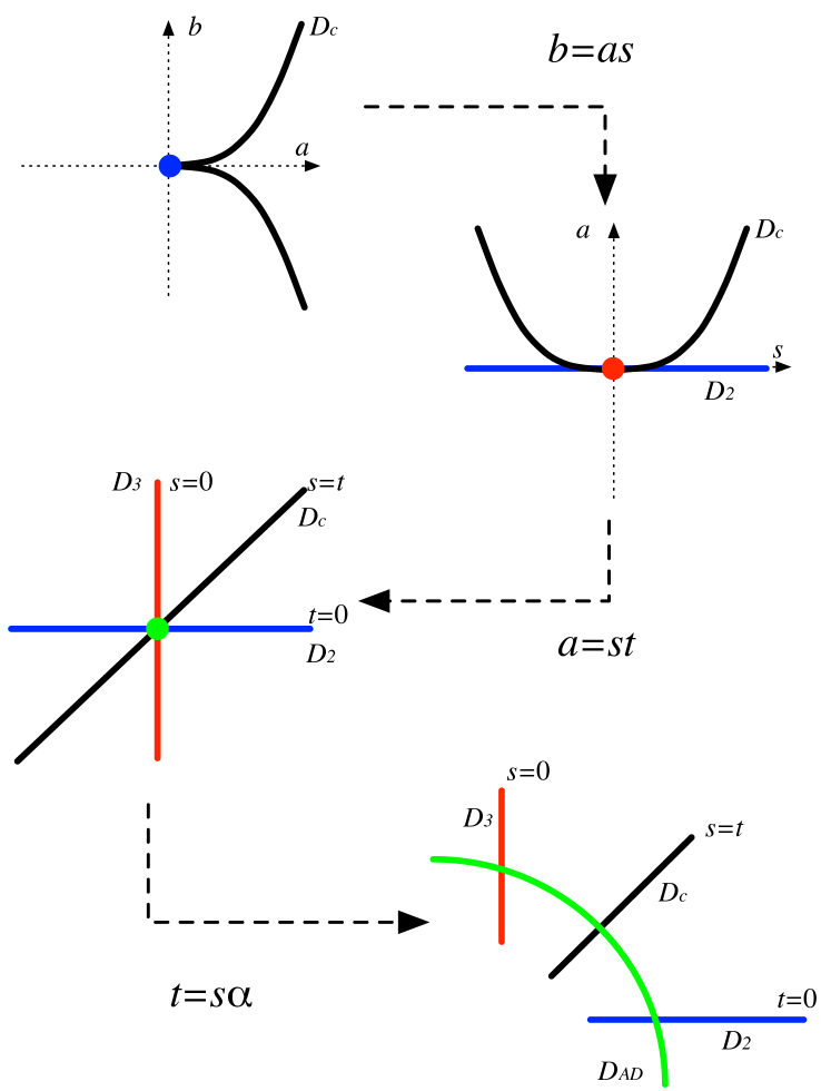
Figure 1: Blowing up of the cusp $b^{2}=a^{3}$

Appendix C Explicit forms of the monodromy matrices

The intersection form of the cycles is

$$\begin{pmatrix}0&-1&0&0&-2&1&0&-1\\ 1&0&0&0&1&-2&1&0\\ 0&0&0&-2&0&1&0&0\\ 0&0&2&0&-1&0&0&0\\ 2&-1&0&1&0&0&0&0\\ -1&2&-1&0&0&0&0&0\\ 0&-1&0&0&0&0&0&0\\ 1&0&0&0&0&0&0&0\end{pmatrix},$$ (C.1)

which is given in eq. (6.32) of ref. [34].

Let us denote the monodromy matrix around the locus $D_{*}$ by $M_{*}$. It is understood they act as

$$(V_{v_{a}},\ldots,T_{t_{b}})^{T}\to M(V_{v_{a}},\ldots,T_{t_{b}})^{T}.$$ (C.2)

where the order and choice of the basis is as in (5.12). Here are the $8\times 8$ matrices:

$$M_{3} =\begin{pmatrix}1&1&0&0&0&0&0&0\\ -1&0&0&0&0&0&0&0\\ 0&0&1&0&0&0&0&0\\ 0&0&0&1&0&0&0&0\\ -2&-1&0&0&1&0&0&0\\ 1&-1&0&0&0&1&0&0\\ 0&1&0&0&0&0&1&0\\ -1&-1&0&0&0&0&0&1\end{pmatrix}, M_{2} =\begin{pmatrix}0&-1&0&0&0&0&0&0\\ 1&0&0&0&0&0&0&0\\ 0&0&1&0&0&0&0&0\\ 0&0&0&1&0&0&0&0\\ 1&-3&0&0&1&0&0&0\\ 1&3&0&0&0&1&0&0\\ -1&-1&0&0&0&0&1&0\\ 1&-1&0&0&0&0&0&1\end{pmatrix},$$ (C.3)

$$M_{c} =\begin{pmatrix}1&1&0&0&0&0&0&0\\ 0&1&0&0&0&0&0&0\\ 0&0&1&0&0&0&0&0\\ 0&0&0&1&0&0&0&0\\ 0&1&0&0&1&0&0&0\\ 0&-2&0&0&0&1&0&0\\ 0&1&0&0&0&0&1&0\\ 0&0&0&0&0&0&0&1\end{pmatrix}, M_{AD} =\begin{pmatrix}-1&0&0&0&0&0&0&0\\ 0&-1&0&0&0&0&0&0\\ 0&0&1&0&0&0&0&0\\ 0&0&0&1&0&0&0&0\\ -2&-4&0&0&1&0&0&0\\ 4&2&0&0&0&1&0&0\\ -2&0&0&0&0&0&1&0\\ 0&-2&0&0&0&0&0&1\end{pmatrix}.$$ (C.4)

References

- [1] R. Bousso and J. Polchinski, “Quantization of four-form fluxes and dynamical neutralization of the cosmological constant,” JHEP 0006 (2000) 006 [arXiv:hep-th/0004134].
- [2] S. B. Giddings, S. Kachru and J. Polchinski, “Hierarchies from fluxes in string compactifications,” Phys. Rev. D 66 (2002) 106006 [arXiv:hep-th/0105097].
- [3] S. Kachru, R. Kallosh, A. Linde and S. P. Trivedi, “De Sitter vacua in string theory,” Phys. Rev. D 68 (2003) 046005 [arXiv:hep-th/0301240].
- [4] M. R. Douglas, “The statistics of string / M theory vacua,” JHEP 0305 (2003) 046 [arXiv:hep-th/0303194].
- [5] K. Dasgupta, G. Rajesh and S. Sethi, JHEP 9908 (1999) 023 [arXiv:hep-th/9908088]; S. Sethi, talk at KITP, UCSB, Nov 20, 1999 [http://online.kitp.ucsb.edu/online/susy_c99/sethi/].
- [6] F. Denef, M. R. Douglas and B. Florea, “Building a better racetrack,” JHEP 0406 (2004) 034 [arXiv:hep-th/0404257].
- [7] D. Robbins and S. Sethi, “A barren landscape,” Phys. Rev. D 71 (2005) 046008 [arXiv:hep-th/0405011].
- [8] P. K. Tripathy and S. P. Trivedi, “D3 brane action and fermion zero modes in presence of background flux,” JHEP 0506 (2005) 066 [arXiv:hep-th/0503072].
- [9] E. Bergshoeff, R. Kallosh, A. K. Kashani-Poor, D. Sorokin and A. Tomasiello, “An index for the Dirac operator on D3 branes with background fluxes,” arXiv:hep-th/0507069.
- [10] D. Lüst, S. Reffert, W. Schulgin and P. K. Tripathy, “Fermion zero modes in the presence of fluxes and a non-perturbative superpotential,” arXiv:hep-th/0509082.
- [11] S. Ashok and M. R. Douglas, “Counting flux vacua,” JHEP 0401 (2004) 060 [arXiv:hep-th/0307049].
- [12] F. Denef and M. R. Douglas, “Distributions of flux vacua,” JHEP 0405 (2004) 072 [arXiv:hep-th/0404116].
- [13] M. R. Douglas, B. Shiffman and S. Zelditch, “Critical points and supersymmetric vacua. III: String/M models,” arXiv:math-ph/0506015.
- [14] B. R. Greene, D. R. Morrison and A. Strominger, “Black hole condensation and the unification of string vacua,” Nucl. Phys. B 451 (1995) 109 [arXiv:hep-th/9504145].
- [15] S. Katz, A. Klemm and C. Vafa, “Geometric engineering of quantum field theories,” Nucl. Phys. B 497 (1997) 173 [arXiv:hep-th/9609239].
- [16] P. C. Argyres and M. R. Douglas, “New phenomena in SU(3) supersymmetric gauge theory,” Nucl. Phys. B 448 (1995) 93 [arXiv:hep-th/9505062].
- [17] P. C. Argyres, M. R. Plesser, N. Seiberg and E. Witten, “New N=2 Superconformal Field Theories in Four Dimensions,” Nucl. Phys. B 461 (1996) 71 [arXiv:hep-th/9511154].
- [18] T. Eguchi, K. Hori, K. Ito and S. K. Yang, “Study of Superconformal Field Theories in Dimensions,” Nucl. Phys. B 471 (1996) 430 [arXiv:hep-th/9603002].
- [19] A. Giryavets, S. Kachru and P. K. Tripathy, “On the taxonomy of flux vacua,” JHEP 0408 (2004) 002 [arXiv:hep-th/0404243].
- [20] J. P. Conlon and F. Quevedo, “On the explicit construction and statistics of Calabi-Yau flux vacua,” JHEP 0410 (2004) 039 [arXiv:hep-th/0409215].
- [21] M. R. Douglas and Z. Lu, “Finiteness of volume of moduli spaces,” arXiv:hep-th/0509224.
- [22] Z. Lu and E. Natsukawa, “On the Weil-Petersson Geometry of Calabi-Yau Moduli,” arXiv:math.DG/0509172
- [23] E. Witten and J. Bagger, “Quantization Of Newton’s Constant In Certain Supergravity Theories,” Phys. Lett. B 115 (1982) 202.
- [24] A. Strominger, “Special Geometry,” Commun. Math. Phys. 133 (1990) 163.
- [25] L. Castellani, R. D’Auria and S. Ferrara, “Special Kähler Geometry: An Intrinsic Formulation From N=2 Space-Time Supersymmetry,” Phys. Lett. B 241 (1990) 57.
- [26] S. Gukov, C. Vafa and E. Witten, “CFT’s from Calabi-Yau four-folds,” Nucl. Phys. B 584 (2000) 69 [Erratum-ibid. B 608 (2001) 477] [arXiv:hep-th/9906070].
- [27] T. R. Taylor and C. Vafa, “RR flux on Calabi-Yau and partial supersymmetry breaking,” Phys. Lett. B 474 (2000) 130 [arXiv:hep-th/9912152].
- [28] A. Todorov, “Weil-Petersson volumes of the moduli spaces of CY manifolds,” arXiv:hep-th/0408033.
- [29] Z. Lu and X. Sun, “Weil-Petersson geometry on moduli space of polarized Calabi-Yau Manifolds,” Journal de l’Institut Mathematique de Jussieu 3 (2004) 185 [math.DG/0510020]
- [30] Z. Lu and X. Sun, “On the Weil-Petersson volume of the moduli space of Calabi-Yau manifolds,” arXiv:math.DG/0510021
- [31] Y. Hayakawa, “Degenaration of Calabi-Yau Manifold with W-P Metric,” arXiv:alg-geom/9507016
- [32] C.-L. Wang, “On the incompleteness of the Weil-Petersson Metric Along Degenerations of Calabi-Yau Manifolds,” Math. Research Lett. 4 (1997) 157
- [33] E. Viehweg, “Quasi-Projective Moduli for Polarized Varieties,” Ergebnisse der Mathematik und ihrer Grenzgebiete, 3. Folge, Band 30, Springer, 1995
- [34] M. Billó, F. Denef, P. Frè, I. Pesando, W. Troost, A. Van Proeyen and D. Zanon, “The rigid limit in special Kähler geometry: From K3-fibrations to special Riemann surfaces: A detailed case study,” Class. Quant. Grav. 15 (1998) 2083 [arXiv:hep-th/9803228].
- [35] W. Schmid, “Variation of Hodge Structure: The Singularities of the Period mapping,” Invent. Math. 22 (1973) 211
- [36] S.-T. Yau, “A Generalized Schwarz Lemma for Kähler Manifolds,” Amer. Jour. Math. 100 (1978) 179