UG-05-07
SPIN-05/30
ITP-UU-05/44

We investigate non-extremal D-instantons in an asymptotically ${\rm AdS_{5}\times S^{5}}$ background and the role they play in the ${\rm AdS_{5}}/{\rm CFT_{4}}$ correspondence. We find that the holographic dual operators of non-extremal D-instanton configurations do not correspond to self-dual Yang-Mills instantons, and we compute explicitly the deviation from self-duality.

Furthermore, a class of non-extremal D-instantons yield Euclidean axionic wormhole solutions with two asymptotic boundaries. After Wick rotating, this provides a playground for investigating holography in the presence of cosmological singularities in a closed universe.

1 Introduction

It is by now well-established that the D-instanton of IIB string theory [1] plays an important role in the calculation of non-perturbative contributions to the low-energy string effective action [2]. Several attempts have been made in the literature to generalize this D-instanton solution [3, 4, 5, 6, 7] to more general instanton solutions of Euclidean IIB supergravity. In a recent work [8] we showed that the extremal and non-extremal D-instantons in (asymptotically) flat space fall under the three conjugacy classes of $SL(2,\mathbb{R})$, the duality symmetry of IIB supergravity. The role of the deformation parameter was played by the determinant of the solutions’ $SL(2,\mathbb{R})$ charge matrix. In some cases the non-extremal instantons can be understood in terms of non-extremal black holes (or $p$-branes) in one (or $p+1$) higher dimension. In other cases, the solutions correspond to axionic Euclidean wormhole geometries with two boundaries that asymptote flat space at infinity [8, 9].

In this paper we extend our investigation of the non-extremal D-instantons to asymptotically Anti-de Sitter spaces. While our analysis can be done in any spacetime dimension, we will focus on the case of ${\rm AdS_{5}}$. This allows us to study their dual description, via the ${\rm AdS_{5}/CFT_{4}}$ correspondence, in the $\mathcal{N}=4$ supersymmetric Yang-Mills theory. For extremal D-instantons in ${\rm AdS_{5}\times S^{5}}$, the dual description in terms of self-dual Yang-Mills instantons has been studied in great detail [10, 11, 12, 13, 14, 15, 16, 17]. To go beyond extremality, this will necessitate to generalize the work of [8] and construct non-extremal D-instantons in an asymptotically ${\rm AdS_{5}\times S^{5}}$ background. Such solutions were also discussed in [7]. In a different context similar solutions were discussed in [18, 19].

After our construction of non-extremal D-instanton solutions in ${\rm AdS_{5}\times S^{5}}$ we calculate the dual operators in the ${\cal N}=4$ gauge theory. Since the supergravity solution is supported by the dilaton and axion, the dual operators are ${\rm Tr}F^{2}$ and ${\rm Tr}F\tilde{F}$ respectively. We will establish that, in contrast to the extremal case, these operators do not satisfy the self-duality constraints for Yang-Mills instantons. The construction of explicit non-self-dual instanton solutions for gauge group $SU(2)$ is notoriously complicated. However, as we will show, for gauge groups $SU(N)$ this is easier and we will suggest that such non-self dual YM instantons are the holographic duals of certain non-extremal D-instantons.

Part of our motivation comes from applications to cosmology. As we will see, some of the non-extremal D-instanton solutions have metrics that describe Euclidean wormholes in Einstein frame. These can be Wick rotated to time-dependent backgrounds with a Big Bang and Big Crunch singularity. A similar situation appeared in [20], whose authors were motivated by the search of holographic duals of closed cosmologies. Moreover, albeit in a slightly different context, non-extremal D-instantons have been discussed in relation to FLRW cosmologies [21].

This paper is organized as follows. In section 2 we shortly review D=10 Euclidean IIB supergravity and its relation, via compactification over S⁵, to the effective D=5 field theory. In section 3 we construct extremal and non-extremal instantons in an ${\rm AdS}_{5}$ background of this effective D=5 field theory. By construction each solution can be uplifted to a D=10 instanton solution in an ${\rm AdS_{5}\times S^{5}}$ background. In section 4 we calculate the corresponding instanton actions. Next, in section 5 we calculate, via the ${\rm AdS_{5}/CFT_{4}}$ correspondence, the operator expressions of the corresponding Yang-Mills 1-point functions. In section 6 we review the correspondence between extremal D-instantons and (anti-) self-dual YM instantons. In the same section we generalize this to the case of non-extremal instantons and propose a possible relation between one class of these instantons and non-self-dual YM instantons. The other class of solutions, however, is less evident to discuss in the AdS/CFT context, but yields interesting cosmological solution after Wick rotation. In section 7 we present our conclusions.

We have added two appendices. In appendix A, we present the path integral formulation of the axion-dilaton system that leads to D-instantons in the semi-classical approximation. In that formalism we can properly explain the ‘wrong’ sign of the axionic kinetic term, the necessary boundary terms in the action and we will see how the analog of the Yang-Mills $\theta$-term arises on the gravity side. In appendix B, we present the D-instanton solutions in $D=3$, in which expressions can be found in closed form.

2 D=10 Euclidean Supergravity

Our starting point is D=10 Euclidean IIB supergravity (see for instance [22]). We only need to consider the metric $g_{\mu\nu}$, the dilaton $\phi$, the axion $\chi$, which is a pseudo-scalar, and the 4-form potential whose 5-form curvature tensor $F_{5}$ in Euclidean space is imaginary self-dual i.e. $\star F_{5}=iF_{5}$. Setting the fermions and the other bosonic fields equal to zero, the equations of motion for these fields are given by:

$$\partial_{\mu}(\sqrt{g}\,e^{2\phi}g^{\mu\nu}\partial_{\nu}\chi)=0\,,$$ (1)

$$\partial_{\mu}(\sqrt{g}\,g^{\mu\nu}\partial_{\nu}\phi)+\sqrt{g}\,e^{2\phi}g^{\mu\nu}\partial_{\mu}\chi\partial_{\nu}\chi=0\,,$$ (2)

$$\mathcal{R}_{\mu\nu}-\tfrac{1}{2}\partial_{\mu}\phi\partial_{\nu}\phi+\tfrac{1}{2}e^{2\phi}\partial_{\mu}\chi\partial_{\nu}\chi-\tfrac{1}{6}F_{\mu}{}^{\mu_{1}\mu_{2}\mu_{3}\mu_{4}}F_{\nu\mu_{1}\mu_{2}\mu_{3}\mu_{4}}=0\,,$$ (3)

$$\partial_{\mu}(\sqrt{g}\,F^{\mu\mu_{1}\mu_{2}\mu_{3}\mu_{4}})=0\,,$$ (4)

where $g={\rm det}\,g_{\mu\nu}$ and $\mathcal{R}_{\mu\nu}$ is the Ricci tensor. This subsector of IIB supergravity supports Euclidean D(-1) and D3 brane solutions. Below, we briefly summarize some features of both solutions. Note that $\chi$ has the ‘wrong’ sign in front of its kinetic term. We explain this in detail in appendix A.

Taking the near horizon limit of the Euclidean D3-brane, the metric becomes that of Euclidean AdS${}_{5}\times$S⁵ and $F_{5}$ takes the form of the Freund-Rubin Ansatz [23]. In Poincaré coordinates this is given by:

$$ds^{2}=\frac{\sqrt{Q_{3}}}{z^{2}}(dz^{2}+d\vec{y}_{4}^{\,2})+\sqrt{Q_{3}}d\Omega_{5}^{2}\,,$$ (5)

$$F_{5}=-\frac{i\hskip 2.56073ptQ_{3}}{z^{5}}\hskip 2.56073ptdz\wedge dy^{0}\wedge dy^{1}\wedge dy^{2}\wedge dy^{3}-\star\,\frac{\hskip 2.56073ptQ_{3}}{z^{5}}dz\wedge dy^{0}\wedge dy^{1}\wedge dy^{2}\wedge dy^{3}\,,$$ (6)

where $Q_{3}$ is proportional to the D3-brane charge. From this expression we notice that the radius $l$ of the 5-sphere and of Euclidean Anti-de Sitter space (EAdS₅) is related to $Q_{3}$ via $l^{2}=\sqrt{Q_{3}}$.

On the other hand the solution for the D(-1)-brane, or extremal D-instanton, in string frame reads:

$$ds^{2}=(H_{-1})^{1/2}(d\rho^{2}+\rho^{2}d\Omega_{9}^{2}),$$ (7)

$$e^{\phi}=H_{-1}\,,$$ (8)

$$d\chi=\pm d(H_{-1})^{-1}\,,$$ (9)

with the harmonic $H_{-1}$ given by:

$$H_{-1}=g_{s}+\frac{Q_{-1}}{\rho^{8}}\,,$$ (10)

where the integration constant $Q_{-1}$ is proportional to the instanton charge and $g_{s}\equiv e^{\phi(\infty)}$.

Since D(-1)-branes correspond to D-instantons, and (stacked) D3-branes are the starting point of the AdS₅/CFT₄ correspondence leading to a duality with $\mathcal{N}=4$ supersymmetric Yang-Mills theory, it is a priori natural to consider intersections of a single D-instanton with a stack of Euclidean D3-branes, and, if possible, to extend this to the case of a non-extremal D-instanton. However, we would like to consider localized intersections as opposed to delocalized intersections involving the extremal D-instanton, which have been considered in [13, 24]. Due to the technical complications with the construction of the appropriate localized brane intersections (no explicit expressions are known, see for instance [25]) we will only consider instanton solutions of the effective D=5 theory that follows after compactification over S⁵, in the rest of this paper. By construction, each of these instanton solutions can be uplifted to a D=10 instanton in an AdS${}_{5}\times$ S⁵ background. What we will not consider is the (localized) brane intersection whose near-horizon geometry gives rise to this D=10 instanton.

The D=5 field theory is obtained as follows. We split the 10-dimensional space into the product of two parts, one with coordinates $x_{\mu}\,,\ \mu=0,\ldots,4\,$, and the other part with coordinates $y_{a}\,,\ a=0,\ldots,4\,$. Next, we consider the following Ansatz:

$$ds^{2}_{10}=g_{\mu\nu}(x)dx^{\mu}dx^{\nu}+g_{ab}(y)dy^{a}dy^{b}\,,$$ (11)

$$\chi=\chi(x),\quad\phi=\phi(x)\,,$$ (12)

$$F_{\mu\nu\rho\sigma\delta}(x)=-\frac{i}{l}\sqrt{{\rm det}g(x)}\,\,{\epsilon}_{\mu\nu\rho\sigma\delta}\,,$$ (13)

$$F_{abcde}(y)=-\frac{1}{l}\sqrt{{\rm det}\,g(y)}\,{\epsilon}_{abcde}\,,$$ (14)

where ${\epsilon}$ is the 5-dimensional Levi-Civita symbol and $l$ is a constant. With this Ansatz the self-duality and equation (4) is satisfied. The Einstein equation (3) is solved in the $y_{a}$-directions provided $g_{ab}(y)$ is the metric of the 5-sphere S⁵ with radius $l$. At this point we are left with the following equations for the metric and the scalars in the $x_{\mu}$-directions:

$$\partial_{\mu}(\sqrt{g}e^{2\phi}g^{\mu\nu}\partial_{\nu}\chi)=0\,,$$ (15)

$$\partial_{\mu}(\sqrt{g}g^{\mu\nu}\partial_{\nu}\phi)+\sqrt{g}e^{2\phi}g^{\mu\nu}\partial_{\mu}\chi\partial_{\nu}\chi=0\,,$$ (16)

$$\mathcal{R}_{\mu\nu}-\tfrac{1}{2}\hskip 2.56073pt\partial_{\mu}\phi\partial_{\nu}\phi+\tfrac{1}{2}\hskip 2.56073pte^{2\phi}\partial_{\mu}\chi\partial_{\nu}\chi-\tfrac{1}{3}\hskip 2.56073ptg_{\mu\nu}\Lambda=0\,,$$ (17)

where $\Lambda=-12/l^{2}$. These equations can be derived from the following effective action:

$$\boxed{S=-\frac{1}{2\kappa_{5}^{2}}\int\,d^{5}x\,\sqrt{g}\Bigl{[}\mathcal{R}-\Lambda-\tfrac{1}{2}\hskip 2.56073pt\partial_{\mu}\phi\partial^{\mu}\phi+\tfrac{1}{2}\hskip 2.56073pte^{2\phi}\partial_{\mu}\chi\partial^{\mu}\chi\Bigr{]}\,.\,}$$ (18)

The 5-dimensional $\kappa_{5}$ is related to the 10-dimensional $\kappa_{10}$ via: $1/\kappa_{5}^{2}=l^{5}\pi^{3}/\kappa_{10}^{2}$.

In the next section we will construct instanton solutions, corresponding to this action.

3 Instanton Solutions

We will present the instanton solutions such that one can read of how the $SL(2,\mathbb{R})$ symmetry acts in the space of instanton solutions. This is done by constructing the $SL(2,\mathbb{R})$ Noether charges of the instanton, as explained in [8]. The charges transform under the adjoint of $SL(2,\mathbb{R})$ and by rewriting the integration constants of the solution as a function of the Noether charges, the transformation properties become clear. All the solutions will have at least $SO(5)\times SO(6)$ symmetry, where the $SO(6)$ part is present from a 10-dimensional point of view. The solutions have the property that in the limit $l\rightarrow\infty$ they reduce to the instanton solutions in a flat background constructed in [8], where $l$ is the characteristic radius of the asymptotically ${\rm AdS_{5}}$ metric.

3.1 The Extremal Instanton

In the extremal case we assume that the metric is that of EAdS₅. This is only possible if the scalars do not contribute to the Euclidean energy-momentum tensor. In such a case one has a solution carrying half of the Euclidean supersymmetries [12]. Taking the trace of (17) and using (16) we find:

$$\partial_{\mu}(\sqrt{g}g^{\mu\nu}\partial_{\nu}e^{\phi})=0.$$ (19)

Therefore $e^{\phi}$ is a harmonic function over EAdS₅. For the axion $\chi$ we then find that:

$$\chi=\pm\Bigl{[}e^{-\phi}+\text{constant}\Bigr{]}\,,$$ (20)

where the + (–) refers to an instanton (anti-instanton). In Poincaré coordinates, the solution reads:

$$\boxed{\begin{aligned} ds^{2}&=\frac{l^{2}}{z^{2}}(dz^{2}+d\vec{y}_{4}^{\,2})\,,\\ e^{\phi}&=|q_{-}|H\,,\\ \chi&=\frac{1}{q_{-}}\Bigl{(}H^{-1}-q_{3}\Bigr{)}\,.\end{aligned}}$$ (21)

In this notation a positive (negative) sign of $q_{-}$ means that the solution is an (anti-) instanton. The harmonic $H$ reads

$$H(z,\vec{y})=\frac{g_{s}}{|q_{-}|}+\frac{4\sqrt{\frac{2}{3}}}{z_{0}^{3}}+\frac{2\sqrt{\frac{2}{3}}(1-2\frac{f^{2}}{z_{0}^{2}})\sqrt{1+\frac{f^{2}}{z_{0}^{2}}}}{f^{3}}\,,$$ (22)

with $f(z,\vec{y})$ defined as the following $SO(1,5)$ invariant function:

$$f(z,\vec{y})=\frac{\sqrt{((z_{0}-z)^{2}+(\vec{y}-\vec{y_{0}})^{2})\hskip 4.2679pt((z_{0}+z)^{2}+(\vec{y}-\vec{y_{0}})^{2})}}{2z}\,.$$ (23)

This harmonic function (22) has a singularity at ($z=z_{0},\,\vec{y}=\vec{y}_{0}$) and this is interpreted as the position of the D-instanton.

The $SL(2,\mathbb{R})$ charge matrix of the solution is defined by integrating over a 4-sphere inclosing the D-instanton :

$$\mathcal{Q}=\frac{1}{2\sqrt{6}Vol(S^{4})}\int_{S^{4}}{J_{\mu}\eta^{\mu}}\,,$$ (24)

where the vector $J_{\mu}$ is the $SL(2,\mathbb{R})$ Noether current which is a $2\times 2$ matrix, and $\eta_{\mu}$ is a unit vector everywhere perpendicular to S⁴. The details are explained in [8], so we immediately go to the result, namely:

$$\mathcal{Q}=\left(\begin{array}[]{cc}q_{3}&iq_{+}\\ iq_{-}&-q_{3}\\ \end{array}\right)\,.$$ (25)

The number $q_{+}$ is some function of the integration constants $q_{-}$ and $q_{3}$. The determinant

$${\rm det}\ \mathcal{Q}=q_{+}q_{-}-q_{3}^{2}\ ,$$ (26)

can be positive or negative. From now on we will use the symbol $q^{2}=-{\rm det}\mathcal{Q}$ in our solutions. The determinant of this matrix equals zero for the extremal instanton solutions i.e. $q^{2}=0$.

Next, we consider the non-extremal instantons that have non-vanishing $q^{2}$. Since the metric is $SL(2,\mathbb{R})$ invariant we expect it to get deformed with the $SL(2,\mathbb{R})$ invariant charge parameter $q^{2}$. The idea is to ‘guess’ a possible deformation for the metric and then construct the whole solution, i.e. the dilaton and the axion. These deformations are most easily found in radial coordinates ($r$, $\theta_{1}$, …, $\theta_{4}$):

$$ds^{2}=\frac{dr^{2}}{1+\frac{r^{2}}{l^{2}}}+r^{2}d\Omega_{4}^{2}.$$ (27)

Partial properties of these solutions were already discussed in [7, 26]. It will be necessary to discuss the cases $q^{2}>0$ and $q^{2}<0$ separately. We refer to them as the super- and sub-extremal instanton respectively. The solutions will have the property that they reduce to the extremal instanton (21) in the limit of $q^{2}\rightarrow 0$.

3.2 The Super-Extremal Instanton: $q^{2}>0$

The solution reads:

$$\boxed{\begin{aligned} ds^{2}&=\frac{dr^{2}}{1+\frac{r^{2}}{l^{2}}+\frac{q^{2}}{r^{6}}}+r^{2}d\Omega_{4}^{2},\\ e^{\phi(r)}&=\,\frac{|q_{-}|}{q}\sinh[qH(r)]\,,\\ \chi(r)&=\frac{1}{q_{-}}\Bigl{(}q\coth[qH(r)]-q_{3}\Bigr{)}\,,\end{aligned}}$$ (28)

where $H(r)$ is a harmonic function on the asymptotically EAdS₅ space, that satisfies

$$\partial_{r}H(r)=-\frac{\sqrt{24}}{g^{rr}\sqrt{g}}\,.$$ (29)

A compact explicit solution of this differential equation is not known in $D=5$, whereas in $D=3$ the situation simplifies as is shown in appendix B. In the limit of vanishing cosmological constant ($l\rightarrow\infty$) everything can be solved explicitly and reduces to the results obtained in [8]. The three integration constants $q,q_{-},q_{3}$ are related to the $SL(2,\mathbb{R})$ charge matrix as is given in (25). The integration constant for $H$ gets fixed in terms of the string coupling constant $g_{s}$ by defining $g_{s}=e^{\phi(\infty)}$. Since the derivative (29) is strictly negative we conclude that $e^{\phi}>0$ for all $r$ if we choose $g_{s}>0$, as it should be. The harmonic function has a singularity at $r=0$ which we identify with the position of the instanton. This position corresponds to $z=l$ and $\vec{y}=0$ in Poincaré coordinates. Since the $SO(1,5)$ symmetry is broken by the deformation to an $SO(5)$ symmetry, there exist less bosonic collective coordinates, resulting in the fact that the singularity (position of the instanton) cannot be moved around in this space.

The coordinate $r$ runs from $r=0$ to $r=\infty$ and this patch covers the whole manifold. At $r=0$ the Ricci scalar blows up ($\mathcal{R}\sim 12q^{2}/r^{8}$) and hence there is a genuine singularity. This is drawn suggestively in figure 1. At this curvature singularity the harmonic has a singularity too and hence the dilaton blows up and we cannot trust the supergravity approximation. One might hope that string theory corrections resolve this singularity. Nonetheless, the solution can be trusted away from the singularity.

For this super-extremal solution there exists an interesting limit for which one rescales the integration constants and then let $q_{-}\rightarrow 0$. This induces a consistent truncation of the axion [8], hence this solution reduces to a solution of a dilaton-gravity system. One ends up with the same metric but now the dilaton reads $\phi=\text{log}(g_{s})+qH$, which is clearly a solution of the dilaton equation $\Box\phi=0$. This deformation of EAdS₅ has been studied before, for instance in [26].

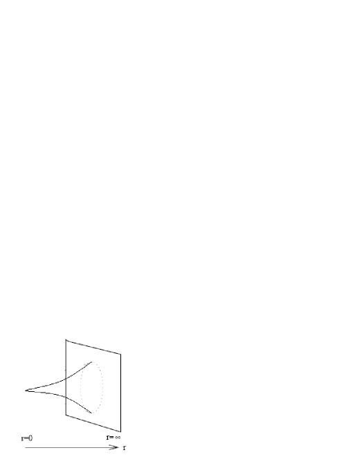
Figure 1: For the class $q^{2}>0$ the space looks like a one-sided wormhole which closes at $r=0$. The plane on the right symbolizes that the solution asymptotes to Euclidean Anti-de Sitter space.

3.3 The Sub-Extremal Instanton: $q^{2}<0$

Now we deal with solutions which have negative $q^{2}$. These solutions share the same symmetry properties as the previous solutions where $q^{2}$ was positive, namely they break the $SO(1,5)$ symmetry of pure EAdS₅ down to a $SO(5)$ symmetry.

Defining $\tilde{q}^{2}=-q^{2}>0$, the sub-extremal instanton solution reads:

$$\boxed{\begin{aligned} ds^{2}&=\frac{dr^{2}}{1+\frac{r^{2}}{l^{2}}-\frac{\tilde{q}^{2}}{r^{6}}}+r^{2}d\Omega_{4}^{2},\\ e^{\phi(r)}&=|\,\frac{q_{-}}{\tilde{q}}\sin[\tilde{q}H(r)]\,|,\\ \chi(r)&=\frac{1}{q_{-}}\Bigl{(}\tilde{q}\cot[\tilde{q}H(r)]-q_{3}\Bigr{)}\,,\end{aligned}}$$ (30)

where $H(r)$ is an harmonic satisfying equation (29) and like in the previous case cannot be obtained explicitly in D=5, whereas in D=3 explicit results are easy to obtain (appendix B). Despite this, it is not hard to check (e.g. numerically) that contrary to the super-extremal instanton, the harmonic is regular.

The coordinates run from $r=r_{c}$ to $r=\infty$, where $r_{c}$ is the unique root of

$$1+\frac{r^{2}}{l^{2}}-\frac{\tilde{q}^{2}}{r^{6}}=0\,.$$ (31)

One can check that $r_{c}$ corresponds to a coordinate singularity because the Ricci scalar $\mathcal{R}$ stays finite at $r=r_{c}>0$ since $\mathcal{R}=-12\tilde{q}^{2}/r_{c}^{8}-20/l^{2}$ . It is possible to resolve this singularity by making a coordinate transformation such that the metric takes the following form:

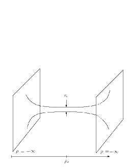
Figure 2: For the class $q^{2}<0$ the space is a wormhole with the neck of the wormhole at $r=r_{c}$ and again the planes represent the fact the geometry asymptotes to pure Euclidean Anti-de Sitter.

$$ds^{2}=d\rho^{2}+a(\rho)^{2}d\Omega_{4}^{2}\,.\\$$ (32)

This implies the relation $a(\rho)=r$. The coordinate $\rho$ goes from $-\infty$ to $+\infty$, and the function $a(\rho)$ can be thought of as the scale factor. From the relations between the two frames we derive an equation for the scale factor :

$$(\partial_{\rho}a)^{2}=1-\frac{\tilde{q}^{2}}{a^{6}}+\frac{a^{2}}{l^{2}}.$$ (33)

The difficulties in $D=5$ encountered in solving this equation explicitly are the same as solving for the harmonic function for this space. Although we do not have an explicit solution this is not a problem since all the necessary information is contained in this differential equation. The most relevant points that can be extracted are that this coordinate system ‘doubles’ the original manifold, and that the scale factor $a(\rho)$ reaches a minimum at $\rho_{c}\equiv\rho(r_{c})$, and that it is even about this point:

$$a(2\,\rho_{c}-\rho)=a(\rho)\,.$$ (34)

Therefore, the sub-extremal D-instanton has the geometry of a wormhole, with its neck at $\rho_{c}$ of size $a(\rho_{c})$. The harmonic function $H$ will acquire the following anti-symmetry:

$$H(2\,\rho_{c}-\rho)=-H(\rho)+2\,H(\rho_{c})\,,$$ (35)

allowing us to easily relate the values of the scalar fields at both asymptotic regions of the wormhole. We can read of from (30) that there is a singularity in the axion and in the derivative of the dilaton whenever $\tilde{q}H(\rho)$ equals a multiple of $\pi$. If the range spanned by the image of $\tilde{q}H$ is smaller than $\pi$ we can always tune $g_{s}$ such that $\tilde{q}H(\rho)$ never reaches a multiple value of $\pi$ (i.e the argument of the sine is on the same branch cut). This range $R$ is given by $R=|\tilde{q}H(\infty)-\tilde{q}H(-\infty)|$. Using (35) and (29) we find:

$$R=2\,\sqrt{24}\,\,\tilde{q}\,\int^{+\infty}_{r_{c}}\frac{1}{r^{4}\sqrt{1-\frac{\tilde{q}^{2}}{r^{6}}+\frac{r^{2}}{l^{2}}}}\,dr\,.$$ (36)

By changing the integration variable to $x=r/l$ one finds that the integrand and the domain of integration only depend on the combination $\tilde{q}^{2}/l^{6}$ and therefore $R$ only depends on that variable. Numerical calculations show that there is no value for $\tilde{q}^{2}/l^{6}$ for which $R<\pi$. Hence there is always a singularity in $\chi$ and in $\phi$, but there is no singularity in $e^{2\phi}$. It can be shown that, for models with a different coupling ‘$b$’ of the dilaton to the axion i.e.

$$\mathcal{L_{\text{SCALAR}}}\sim(\partial\phi)^{2}-e^{b\phi}(\partial\chi)^{2}\,,$$ (37)

there exist solutions which are regular in $\chi$ and $\phi$, when $b<\sqrt{8/3}$. Such values for the dilaton coupling constant could for instance be obtained from non-spherical compactifications. For the case of zero cosmological constant, this can be achieved in Calabi-Yau compactifications of type II strings, as was demonstrated in [9].

3.4 Lorentzian Solutions

Until now we presented three solutions ($q^{2}>0$, $q^{2}=0$ and $q^{2}<0$) of the Euclidean IIB action involving five-form flux, the dilaton- and the axion-field. But this subsector of IIB supergravity also holds interesting solutions of the Lorentzian theory. One way to try to obtain these solutions is by Wick rotating the Euclidean solutions and to check whether they are solutions of the Lorentzian theory. As pointed out in [20] Euclidean wormholes can Wick rotate to Big Bang/Big Crunch cosmologies and as we will show this is indeed what happens in our case. The extremal and super-extremal solution cannot be Wick rotated to real solutions of Lorentzian IIB supergravity.

The Wick rotation proceeds by considering the sub-extremal solution in the $\rho$-coordinates and taking $\rho=i\tau$. We can always shift the $\rho$-coordinates such that the neck is located at the origin. Doing so the Euclidean scale factor $a_{E}(\rho)$ is an even function and can be Wick rotated to a real function i.e $\,a_{L}(\tau)\,:=\,a_{E}(i\tau)\,\,\in\,\,\mathbb{R}$. The metric Ansatz becomes the following cosmology:

$$ds^{2}=-d\tau^{2}+a_{L}(\tau)^{2}d\Omega_{4}^{2}\,.$$ (38)

The function $a_{L}(\tau)$ is called the Lorentzian scale factor. Wick rotating the fields is somewhat more involved. One first has to notice that (up to an additive constant) $H_{E}(\rho)\rightarrow iH_{L}(\tau)$, where $H_{E}$ and $H_{L}$ are the harmonic functions over the Euclidean and Lorentzian geometry respectively. One has the freedom to Wick rotate the integration constants as long as one ends up with a real dilaton field $\phi(\tau)$, and the axion field $\chi(\tau)$ should get an extra factor of $i$ during the Wick rotation. These Wick rotation rules are:

$$q_{3} \rightarrow iq_{3}\,,$$ (39)

$$H_{E} \rightarrow iH_{L}+\frac{\pi}{2}\,.$$ (40)

The second rule is necessary to keep the dilaton field real and is to be interpreted as a Wick rotation rule for the integration constant belonging to the definition of the harmonic function $H_{E}$. The solution we end up with reads:

$$\boxed{\begin{aligned} ds^{2}&=-d\tau^{2}+a^{2}_{L}(\tau)d\Omega_{4}^{2}\,,\\ e^{\phi(\tau)}&=\,\frac{|q_{-}|}{\tilde{q}}\cosh[\tilde{q}H_{L}(\tau)]\,,\\ \chi(\tau)&=\frac{1}{q_{-}}\Bigl{(}\tilde{q}\tanh[\tilde{q}H_{L}(\tau)]+q_{3}\Bigr{)}\,.\end{aligned}}$$ (41)

The $l\rightarrow\infty$ version of this solution was studied in [27]. To check that this is a solution one has to use the Lorentzian field equations which give for the scale factor (after combining the Einstein equation with the scalar field equations) :

$$(\partial_{\tau}a_{L})^{2}=-\Bigl{[}1-\frac{\tilde{q}^{2}}{a_{L}^{6}}+\frac{a_{L}^{2}}{l^{2}}\Bigr{]},$$ (42)

which differs with an overall minus sign from the equation for the Euclidean scale factor $a_{E}(\rho)$ (33). One can check that the Wick rotated scale factor $a_{L}(\tau):=a_{E}(i\tau)$ indeed obeys this equation. The same holds for the scalar fields; straightforwardly putting them in the Lorentzian field equations shows that (41) indeed is a solution.

This cosmology is a Big Bang/Big Crunch cosmology. This can be seen either by analyzing the scale factor $a_{L}(\tau)$ numerically or by deducing from (42) that a solution has to obey

$$\partial_{\tau}a_{L}=\left\{\begin{array}[]{l}-\sqrt{-1+\frac{\tilde{q}^{2}}{a_{L}^{6}}-\frac{a_{L}^{2}}{l^{2}}}\ \,\,\,\,\quad\text{for}\,\tau>0,\\ \quad\quad 0\qquad\qquad\qquad\quad\,\,\text{for}\,\tau=0,\\ +\sqrt{-1+\frac{\tilde{q}^{2}}{a_{L}^{6}}-\frac{a_{L}^{2}}{l^{2}}}\ \quad\,\,\,\,\,\text{for}\,\tau<0.\end{array}\right.$$ (43)

Between the Big Bang and Big Crunch singularities the scalar fields are completely regular as one can verify. However, at the singularities, the harmonic function blows up.

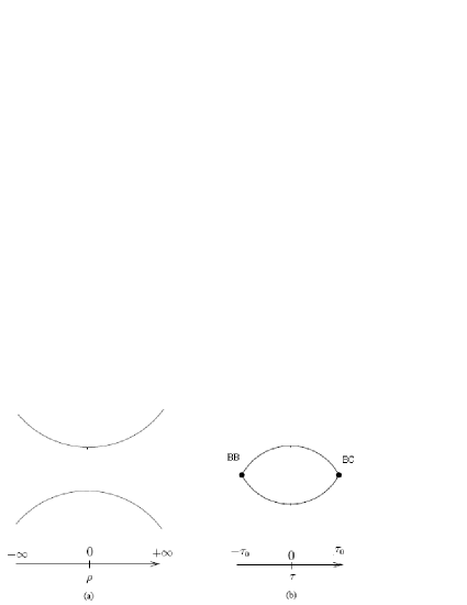
Figure 3: Pictorial description of the effect of Wick rotating a Euclidean wormhole.

As noted at the end of the section on the super-extremal solution ($q^{2}>0$), one can take a limit in which the axion becomes a constant such that the geometry is carried only by a dilaton. Although this is not possible for the Euclidean sub-extremal solution, it is possible for the Lorentzian sub-extremal solution where again the dilaton becomes proportional to the harmonic function. Such a solution has been discussed in [28].

4 Instanton Actions

As explained in appendix A, in order to calculate the on-shell instanton action it is convenient to use the Hodge dual formalism of the axion-dilaton sector of $D=10$ Euclidean IIB supergravity. This dual theory contains a 9-form $F_{9}$ field strength instead of a 1-form field strength $d\chi$. The D-instanton is magnetically charged with respect to this 9-form. We use the following Euclidean action:

$$S=-\frac{1}{2\kappa^{2}_{10}}\int d^{10}x\sqrt{g}\Bigl{[}\mathcal{R}-\tfrac{1}{2}(\partial\phi)^{2}-\tfrac{1}{2}e^{-2\phi}F_{9}^{2}\Bigr{]}\,.$$ (44)

Reducing the theory over S⁵ and using the field equations one finds:

$$S=\underbrace{-\frac{1}{2\kappa^{2}_{5}}\Bigl{(}\int_{M}d^{5}x\,\sqrt{g}\left(\frac{-8}{l^{2}}\right)+2\int_{\partial M}d^{4}x\sqrt{h}K\Bigr{)}}_{S_{\text{GRAV}}}-\underbrace{\frac{1}{2\kappa^{2}_{5}}\int_{M}d^{5}x\,\partial_{\mu}(\sqrt{g}g^{\mu\nu}\partial_{\nu}\phi)}_{S_{\text{SCALAR}}}$$ (45)

We split the action in a part $S_{\text{GRAV}}$ which only contains the metric and a part only involving the dilaton $S_{\text{SCALAR}}$. In the gravitational part $S_{\text{GRAV}}$ we have included the usual Gibbons-Hawking term, where $h_{\mu\nu}$ is the corresponding induced boundary metric $h_{\mu\nu}=g_{\mu\nu}-n_{\mu}n_{\nu}$ and $K$ is the extrinsic curvature w.r.t. $h_{\mu\nu}$. The gravitational part gives an infinite answer and therefore needs to be regularized. For clarity we discuss $S_{\text{GRAV}}$ and $S_{\text{SCALAR}}$ separately.

Since $S_{\text{SCALAR}}$ is a total derivative we use Stokes theorem. After integration over the angles one finds the following term:

$$S_{\text{SCALAR}}=-\frac{1}{2\kappa_{5}^{2}}\text{Vol}(S^{4})\eta^{r}r^{4}\partial_{r}\phi\mid_{\partial}\,,$$ (46)

where $\mid_{\partial}$ means that the expression is evaluated at the boundary $\partial$ and $\eta$ is a unit vector perpendicular to the boundary $\partial$. Using (29) this can be rewritten as:

$$S_{\text{SCALAR}}=\frac{\sqrt{24}}{2\kappa_{5}^{2}}\,\text{Vol}(S^{4})\,e^{-\phi(H)}\partial_{H}e^{\phi(H)}\mid_{\partial}\,.$$ (47)

This formula is useful because it only requires the knowledge of the value of $H$ at the boundary and this is completely fixed by fixing $g_{s}$ on the boundary. When we have multiple boundaries as for wormholes we have to subtract the values at different boundaries if the fields are regular everywhere in the bulk.

If we assume that for the super-extremal instanton, the singularity gets resolved by string theory effects, then there is only one boundary at $r=\infty$. This gives:

$$S_{\text{SCALAR}}=\frac{\sqrt{6}\,\text{Vol}(S^{4})}{\kappa_{5}^{2}}\,\sqrt{(\frac{q_{-}}{g_{s}})^{2}+q^{2}}\,.$$ (48)

To obtain the result for the extremal D-instanton we just put $q^{2}=0$ in the above expression.

For the sub-extremal solution we find that the singularities in the fields are not integrable. Hence $S_{\text{SCALAR}}$ formally diverges. The situation can again be improved by having different values of the dilaton coupling parameter $b$. As mentioned in the previous section, this can yield completely regular solutions also for the scalar fields which will result in a finite-action instanton. For zero cosmological constant, this was shown in [8].

Now we focus on $S_{\text{GRAV}}$. The correct way for calculating the on-shell action for gravitational instantons in an asymptotically EAdS space requires infrared renormalization [29, 30]. The reason is that the bulk action diverges because of the integration over a non-compact space. Also the Gibbons-Hawking term diverges since there is a second order pole in the induced boundary metric $h_{\mu\nu}$. This means that one has to add counterterms on the regulating surface $\partial M$ defined by $r=L$. These counterterms cancel the divergences after taking the regulator $L$ to infinity. The action with the counterterms is given by:

$$\begin{split}S_{\text{GRAV}}=&-\frac{1}{2\kappa_{5}^{2}}\int_{M}d^{5}x\sqrt{g}\Bigl{(}\frac{-8}{l^{2}}\Bigr{)}-\frac{1}{\kappa_{5}^{2}}\int_{\partial M}d^{4}x\sqrt{h}K\\ &+\frac{1}{\kappa_{5}^{2}}\int_{\partial M}d^{4}x\sqrt{h}\Bigl{(}\frac{3}{l}+\frac{l}{4}\mathcal{R}_{h}\Bigr{)}+\frac{1}{\kappa_{5}^{2}}\int_{\partial M}d^{4}x\,\sqrt{h}\,a_{4}(h)L^{4}\log{\frac{l}{L}}\,.\end{split}$$ (49)

The last counterterm cannot be written in a covariant way and explicitly contains the regulator. The coefficient $a_{4}$ is a covariant function of the induced metric and gives rise to the conformal anomaly of the dual field theory [30]. This dual field theory lives on a space with a metric that is different from the induced metric $h$, namely the poles have to be dropped such that we get the canonical S⁴ metric with radius $l$. If we would have carried out the same procedure in Poincaré coordinates (instead of radial coordinates) where the regulating surface is defined by $z=1/L$ we would find that $a_{4}$ would be zero. The metric on the dual field theory would be that of $\mathbb{R}^{4}$ on which $\mathcal{N}=4$ SYM has no conformal anomaly. The meaning of this is that the regularization procedure picks out a certain induced metric which will give the metric on which the dual CFT is defined, after the poles of the induced metric are dropped.

This procedure shows that for the super-extremal solution we get some extra but finite terms in the action on top of the finite term generated by pure EAdS₅. These extra terms of course vanish in the limit of $q^{2}\rightarrow 0$. The finite term generated by pure EAdS₅ can be put to zero by making an explicit choice for the scheme dependence of the regularization procedure. Finally notice that $S_{\text{GRAV}}$ does not depend on $g_{s}$, so its contribution does not interfere with the leading semiclassical (in $g_{s}$) contribution from $S_{\text{SCALAR}}$.

5 The ${\rm AdS}_{5}/{\rm CFT}_{4}$ Correspondence

First we will give some basic facts about the ${\rm AdS}_{5}/{\rm CFT}_{4}$ correspondence which are needed to understand what our solutions mean in the dual theory. More explanation can be found in for example [31].

5.1 Generalities

On the string theory side we are working in the supergravity approximation. This means that we assume that $g_{s}N$ is large, while $g_{s}$ stays small, i.e. $1<<g_{s}N<N$. The number $N$ is proportional to the 5-form flux and can be seen as the number of 3-branes sourcing this flux. More specific, we have the relations:

$$l^{4}=Q_{3}=4\pi g_{s}N\alpha^{\prime 2}\,.$$ (50)

According to the duality $g_{YM}^{2}N=4\pi Ng_{s}>>1$ hence we are dealing with a strongly coupled Yang-Mills theory. The $\rm AdS/CFT$ duality equates the generating functions of the dual theories :

$$Z[J=\Phi_{\partial}]=\int\,d[\mathcal{A}]\,\text{exp}\,(-S_{\text{YM}}+J\,\mathcal{O[A]})\,\approx e^{-S_{\text{SUGRA}}[J]}.$$ (51)

Here $\mathcal{O[A]}$ represents a gauge invariant SYM operator which couples to the boundary value of the dual supergravity field $J=\Phi_{\partial}$. The boundary value $\Phi_{\partial}$ then clearly acts as a source in the SYM theory. The fact that the string (supergravity) partition function only depends on $J=\Phi_{\partial}$ is only correct for bulk configurations which are sufficiently regular. This duality (51) allows us to find the 1-point functions of the strongly coupled SYM theory, since

$$-\frac{\delta}{\delta J}\,S_{\text{SUGRA}}[J]=\langle\,\mathcal{O[A]}\,\rangle_{J}.$$ (52)

For the dilaton field $\phi$ and the axion field $\chi$ the dual operators are respectively $\text{Tr}F^{2}+\ldots$ and $\text{Tr}(F\tilde{F})$. To be more specific, using the relations $4\pi g_{s}=g^{2}_{YM},\,\chi_{\infty}=\tfrac{\theta_{YM}}{2\pi}$ and conventions in which the Yang-Mills action looks like

$$S_{YM}=-\frac{1}{4{g_{\text{YM}}}^{2}}\int d^{4}x\text{Tr}(F^{2})+\ldots-i\frac{\theta}{32\pi^{2}}\int d^{4}x\,\text{Tr}(F\tilde{F})\,,$$ (53)

we conclude that:

$$\frac{\delta}{\delta\phi_{\partial}}S=\frac{1}{4{g_{\text{YM}}}^{2}}\langle\text{Tr}F^{2}\rangle+\ldots,$$ (54)

$$\frac{\delta}{\delta\chi_{\partial}}S=-\frac{1}{16\pi}\langle\text{Tr}(F\tilde{F})\rangle,$$ (55)

where the $\ldots$ in the first line can be dropped if no other fields then the vectors are excited.

In general when studying deformations of AdS${}_{5}\times$ S⁵ caused by the backreaction of some matter fields, it affects the dual description in two possible ways. In one case the deformation causes the dual field theory to gain certain vacuum expectation values for Yang-Mills operators which are dual to these matter fields. This is sometimes referred to as a ‘vev-deformation’. The other possibility is an ‘operator deformation’ in which the theory is changed by adding certain operators to the lagrangian. It can be argued as follows that the deformations we are considering are vev-deformations. We mentioned that the boundary value of a bulk field acts as a source for an operator in the dual field theory, so generically $\mathcal{N}=4$ SYM gets deformed by some operator which couples to that source. However if the operator dual to the bulk fields is the lagrangian itself the situation is different. This is of course the case here since the dilaton couples to the real part of the lagrangian ($\sim 1/g^{2}_{\text{YM}}$Tr$F^{2}+\ldots$) and the axion to the imaginary part ($\sim i\theta_{\text{YM}}$Tr$F\tilde{F}$). The above leads one to believe that axion-dilaton deformations do not alter the dual theory but rather pick out a non trivial vacuum (background) which can spontaneously break (parts of) the conformal symmetry and supersymmetry. These arguments are not sufficient because they would imply that all axion-dilaton deformations of (E)AdS (with undeformed S⁵) are dual to vev-deformations of $\mathcal{N}=4$ SYM. A well understood example where this is not the case is the Janus solution [32]. This is a simple dilatonic deformation but the dual theory is marginally deformed. There the reason was that the coupling constant on the boundary makes a discontinuous step which for instance causes the dual theory to lose supersymmetry [33]. In our case the dilaton is constant at the boundary and this phenomenon does not occur, but the example teaches us that one in general has to be careful.

We shortly give an explanation on how to calculate a variation with respect to a boundary value in order to calculate the expectation values. Consider a variation of the action $S=\int L(\Phi,\partial\Phi)$:

$$\delta S=\int[(\frac{\partial L}{\partial\Phi}-\partial\frac{\partial L}{\partial\partial\Phi})\delta\Phi+\partial(\frac{\partial L}{\partial\partial\Phi}\delta\Phi)]\,.$$ (56)

The first part is the equation of motion for the field $\Phi$ and hence disappears on-shell. Using Stokes on the second term we find:

$$\delta S=\int_{\partial}[\eta(\frac{\partial L}{\partial\partial\Phi}\delta\Phi)],$$ (57)

where $\eta$ is a unit vector perpendicular to the boundary $\partial$. Expression (57) is clearly an integral over the boundary of our space. Hence $\delta\Phi$ in the integrand can be replaced by its value on the boundary $\delta\Phi_{\partial}$. From this we read of that,

$$\frac{\delta S}{\delta J(\vec{y})}=\eta_{\mu}\frac{\partial L}{\partial\partial_{\mu}\Phi}(\vec{y}).$$ (58)

How to do this properly for $\rm EAdS_{5}$ is explained for instance in [35]. In general one has to use a regularization technique in order to get finite answers. In practice, this amounts to making a series expansion of the supergravity field in the coordinate $z$[36]:

$$\Phi(\vec{y},z)\approx z^{(4-\Delta)}\Phi(\vec{y})_{\partial}+\ldots+z^{\Delta}\Phi(\vec{y})_{\,(2\Delta-4)}+\ldots\,,$$ (59)

where $\Delta$ is the conformal weight of the dual operator which is related to the mass of the supergravity field $\Phi$. For massless fields such as the axion and the dilaton $\Delta=4$. $\Phi_{\partial}$ represents the source for the dual operator in the field theory, whereas $\Phi_{\,(2\Delta-4)}$ is related to the vacuum expectation value of the dual operator. So the presence of $\Phi_{\partial}$ in general signals an operator deformation, unless $\Delta=4$ where the situation is more subtle. In fact, our deformations are expected to be vev-deformations as explained above.

5.2 Calculation of the 1-point Functions

Until now we gave the non-extremal solutions in radial coordinates but for this section it becomes preferable to present the results in Poincaré coordinates since then the coordinates of the dual field theory are the usual Cartesian coordinates. In the Poincaré coordinate system we approach the boundary by taking small $z$ values and then the Cartesian $y$-coordinates parameterize the surface approaching the boundary.

For the $\rm AdS_{5}/CFT_{4}$ correspondence one needs to know how the dilaton and axion behave near the boundary, i.e. near $z=0$. For the non-extremal solutions there is no explicit expression for the harmonic but since only the behavior near the boundary is of importance we can use perturbation theory. For small $z$ we find:

$$\phi(z,\vec{y})\approx\log[{g_{s}}]+\frac{8\sqrt{6}l{\sqrt{q_{-}^{2}+q^{2}{g_{s}}^{2}}}}{g_{s}(l^{2}+\vec{y}^{\,2})^{4}}\,z^{4}+\mathcal{O}(z^{6})\ ,$$ (60)

$$\chi(z,\vec{y})\approx{g_{s}}^{-1}\sqrt{1+\frac{q^{2}{g_{s}}^{2}}{{q_{-}^{2}}}}-\frac{q_{3}}{{q_{-}}}-\frac{8\sqrt{6}lq_{-}}{(l^{2}+\vec{y}^{\,2})^{4}{g_{s}}^{2}}\,z^{4}+\mathcal{O}(z^{6})\ .$$ (61)

In order to understand the holographic dual of these instantons we have to take the quantization of the axion shift symmetry into account. It will turn out that the dual statement is the fact that the winding number of the YM instanton is an integer. The Noether current associated to the shift symmetry of the axion is

$$\mathcal{J_{\mu}}=e^{2\phi}\partial_{\mu}\chi\ .$$ (62)

Since the exact duality group of type IIB string theory is expected to be $SL(2,\mathbb{Z})$, the $\mathbb{R}$ shift symmetry of $\chi$ is broken to a $\mathbb{Z}$ shift symmetry, i.e. $\chi$ is periodically identified. As we show in appendix A, this leads to the following quantization of the axionic charge:

$$2\pi n=\frac{\pi^{3}l^{5}}{2\kappa_{10}^{2}}\int\mathrm{d}\Sigma^{\mu}e^{2\phi}\partial_{\mu}\chi\,,$$ (63)

resulting in

$$q_{-}=\frac{\sqrt{3/2}\kappa_{10}^{2}}{4\pi^{4}l^{5}}\,n\,.$$ (64)

Now we can apply the formula for the 1-point function to the super-extremal ($q^{2}>0$) and extremal ($q^{2}=0$) instanton, to obtain:

$$\boxed{\begin{aligned} \langle\text{Tr}F^{2}\rangle&=-\frac{192\,l^{4}}{(l^{2}+\vec{y}^{\,2})^{4}}\sqrt{n^{2}+\frac{32\pi^{8}q^{2}g_{s}^{2}l^{10}}{3\kappa_{10}^{4}}},\\ \langle\text{Tr}F\tilde{F}\rangle&=-\frac{192\,l^{4}}{(l^{2}+\vec{y}^{\,2})^{4}}\,n\ .\end{aligned}}$$ (65)

These expressions show that when $q^{2}>0$ we have a field strength $F$ which is not (anti-) self-dual.

For the sub-extremal solution we could naively use (54) on both sides of the wormhole to obtain a result like (65) but now for $q^{2}<0$. That result is simply impossible since it violates the Cauchy-Schwarz inequality $-\text{Tr}F^{2}\geq-\text{Tr}F\tilde{F}$. The reason for this could be twofold; for multiple boundaries one has to calculate 1-point functions differently or another reason could be that the singularity in the axion and dilaton are responsible for this result.

6 The D-instanton / YM Instanton Correspondence

In this section we will discuss the correspondence between D-instantons and Yang-Mills instantons. We explain this correspondence from the point of view of the expectation values for the operators Tr$F^{2}$ and Tr$F\tilde{F}$ as was done for extremal instantons in [35]. We first discuss this for an extremal single-centered D-instanton with charge $q_{-}$, and then extend this to the non-extremal case where $q^{2}>0$. The case of $q^{2}<0$ is more subtle since the bulk geometry has two boundaries. Holography with multiple boundaries is much less well understood; we comment on it at the end of this section.

6.1 The extremal case: $q^{2}=0$

From (65) we have for $q^{2}=0$:

$$\langle\text{Tr}F^{2}\rangle=-\frac{192\,l^{4}}{(l^{2}+\vec{y}^{\,2})^{4}}\,|n|=\pm\langle\text{Tr}F\tilde{F}\rangle\,.$$ (66)

However (65) can be generalized for extremal D-instantons since one can place the position at an arbitrary point of EAdS₅ whereas this is not possible for the non-extremal solutions. If we take the harmonic as in (22) then this results in the more general expression :

$$\langle\text{Tr}F^{2}\rangle=-\frac{192\,z_{0}^{4}}{(z_{0}^{2}+(\vec{y}-\vec{y_{0}})^{2})^{4}}\,|n|=\pm\langle\text{Tr}F\tilde{F}\rangle\,.$$ (67)

For $n=1$ ($n=-1$) this exactly equals the expression for a classical (anti-)self-dual Yang-Mills instanton with size $z_{0}$ placed in flat Euclidean space at a position $\vec{y_{0}}$ in Cartesian coordinates. For $n>1$, the expression in (67) corresponds to a particular self-dual multi-instanton configuration, which we specify below. Observe first that this expression is only the result for the one-point function $\text{Tr}F^{2}$ in the large $N$ limit of the gauge theory at strong ’t Hooft coupling. For large values of $N$, it was shown in [15, 16] that to leading order in the saddle-point expansion:

• The $n$-instanton configuration becomes dominated by $n$ single instantons living in $n$ mutually commuting $SU(2)$ subgroups of $SU(N)$.

• Each of these single instantons are driven to sit at the same point in moduli space, i.e. their positions and sizes are equal.

The expression in (67) is completely consistent with these results. Based on this, we can schematically write down the gauge field

$$A_{\mu}^{SU(N)}(n)=\left(\begin{array}[]{ccccc}A_{\mu}^{SU(2)}(1)&&&0&\\ &A_{\mu}^{SU(2)}(1)&&&\\ &&\ddots&&\\ 0&&&A_{\mu}^{SU(2)}(1)&\\ &&&&\ddots\\ \end{array}\right)\ ,$$ (68)

where $A_{\mu}^{SU(2)}(1)$ stands for a self-dual $SU(2)$ connection with instanton number one.

Notice that also the values of the action coincide since combining (48) with (64) we find that (when $\theta_{\text{YM}}=0$):

$$S_{\text{SUGRA}}=S_{\text{YM}}=\frac{8\pi^{2}}{g^{2}_{YM}}\,|n|\ .$$ (69)

For $\theta\neq 0$ the YM action gets a contribution of the form $i\,\theta\,n$, and in appendix A we will see that the SUGRA action gets a contribution of the form $i\,\chi_{\infty}\,q_{-}$, which can be regarded as the AdS/CFT partner of the YM topological term, since $\chi_{\infty}$ is identified with $\theta$ and $q_{-}$ with $n$. As a final remark we like to emphasize that the matching of D-instanton configurations with self-dual Yang-Mills configurations is actually a surprising result. This is because the D-instanton result yields quantities in the gauge theory at strong ’t Hooft coupling. Instantons in the gauge theory however, are semiclassical objects that are only useful in the weakly coupled regime. The fact that we get results for the one-point function (67) that are easy to interpret in the weakly coupled gauge theory, hints toward a non-renormalization theorem that protects the (semi-) classical value for $\text{Tr}F^{2}$ from perturbative quantum corrections [38].

6.2 The non-extremal case: $q^{2}>0$

We now consider the case of the super-extremal deformation, with $q^{2}>0$. This D-instanton solution is not BPS, and hence we must be careful interpreting the corresponding operators and correlation functions on the gauge theory side, since there is no reason to expect any mechanism that protects quantities from receiving quantum corrections. The strategy we follow here is to stay close to the BPS point, and to consider the case where $q^{2}$ is very small. This is somewhat similar to the description of near-extremal black holes. In fact, in [8] we showed that when the $q^{2}>0$ instanton solution in asymptotically flat space can be uplifted to one higher dimension, it corresponds to a black hole with charge $Q$ and mass $M$ with $4q^{2}=M^{2}-Q^{2}$. The near-extremal black hole then indeed corresponds to taking $q^{2}<<1$. One might hope that for $q^{2}$ very small, the result will not differ too much from the extremal point where the gauge theory interpretation is well understood in terms of $n$ single Yang-Mills instantons sitting at the same point in moduli space.

In the presence of a non-vanishing $q^{2}$, we have seen in (65) that the result for $\text{Tr}F\tilde{F}$ remains the same whereas $\text{Tr}F^{2}$ does get deformed. Consequently, these operators do no longer obey the self-duality relation as for extremal instantons. Stated differently, the field strength still has boundary conditions belonging to the same topological class, labelled by the instanton number $n$, but it has an anti-self-dual component proportional to $q^{2}$. Using (64) as a definition of $n$, the deviation from self-duality can be written as

$$\langle\text{Tr}F^{2}\rangle-\langle\text{Tr}F\tilde{F}\rangle = -\frac{192l^{4}}{(l^{2}+\vec{y}^{\,2})^{4}}\,n\,\Big{(}\sqrt{1+\frac{q^{2}g_{s}^{2}}{q_{-}^{2}}}-1\Big{)}\ ,$$ (70)

$$\approx -\frac{192l^{4}}{(l^{2}+\vec{y}^{\,2})^{4}}\,n\,q^{2}\,\Big{(}\frac{g_{s}^{2}}{2q_{-}^{2}}+O(q^{2})\Big{)}\ ,$$

where in the second line we have expanded for small $q^{2}$. This is the result of the supergravity approximation. We now attempt to give an interpretation in the gauge theory. As already stressed before, one must be careful in giving an interpretation in the weakly coupled gauge theory, since we do not expect that (70) can be extrapolated from strong to weak ’t Hooft coupling, unless perhaps for very small values of $q^{2}$. Because in the non-extremal case there is a (small) anti-self-dual part of the field strength, it is tempting to associate the deformation with the presence of anti-instantons. The description of instanton - anti-instanton configurations in gauge theory is difficult, as there are no known analytic solutions of the second order equations of motion that are not self-dual, at least for gauge groups $SU(2)$ and $SU(3)$. One can work in the dilute gas approximation where instantons are widely separated, but this approximation is not valid for the AdS/CFT correspondence, already in the extremal case. Luckily, for higher rank gauge groups, the situation simplifies. For large values of $N$ one can still consider the configuration (68), but we can deform it by bringing in $SU(2)$ anti-instantons on the diagonal. Such configurations satisfy the second order equations of motion, but are not self-dual. The total instanton charge is still given by $n$, but we distribute it over $k_{+}$ instantons and $k_{-}$ anti-instantons with $n=k_{+}-k_{-}$ and $k_{-}$ small:

$$A_{\mu}^{SU(N)}(n)=\left(\begin{array}[]{cccc}A_{\mu}^{SU(2)}(1)&&&0\cr&\ddots&&\cr&&A_{\mu}^{SU(2)}(1)&\cr 0&&&A_{\mu}^{SU(2)}(-k_{-})\cr\end{array}\right)\ .$$ (71)

Here $A_{\mu}^{SU(2)}(-k_{-})$ stands for an anti-self-dual $SU(2)$ connection with instanton number $-k_{-}$. We have taken all the instantons and anti-instantons at the same point and with the same size, say at ${\vec{y}}_{0}=0$ and $z_{0}=l$, where the (partial) annihilation between instantons and the anti-instanton takes place. One could further distribute the anti-instanton sector into $k_{-}$ single charge anti-instantons, but we will not do so in order to avoid notational complications and because we take $k_{-}$ small w.r.t. $n=k_{+}-k_{-}$ (e.g. $k_{-}=1$). The presence of an anti-instanton in a background of instantons of course leads to an instability. The solution corresponding to (71) is only a saddle point in the path integral, and the annihilation of anti-instanton charge will result in perturbative fluctuations around a local minimum consisting of instanton charge only. We expect a similar instability on the supergravity side.

With this instanton configuration, we can compute the operators

$$\text{Tr}F^{2} = -\frac{192z_{0}^{4}}{(z_{0}^{2}+(\vec{y}-\vec{y_{0}})^{2})^{4}}\,(k_{+}+k_{-})\ ,$$

$$\text{Tr}F\tilde{F} = -\frac{192z_{0}^{4}}{(z_{0}^{2}+(\vec{y}-\vec{y_{0}})^{2})^{4}}\,(k_{+}-k_{-})\ .$$ (72)

Using the fact that $n=k_{+}-k_{-}$, for $z_{0}=l,\vec{y}_{0}=0$, the operator $\text{Tr}F\tilde{F}$ matches with the supergravity prediction, while $\text{Tr}F^{2}$ matches if we identify

$$\frac{k_{-}}{n}=\frac{q^{2}g_{s}^{2}}{4q_{-}^{2}}\ ,$$ (73)

to leading order in the small $q^{2}$ expansion. The left hand side is a rational number. For this identification to make sense, we must understand better the quantization condition on $q^{2}g_{s}^{2}$. This issue can however not be addressed in the supergravity approximation that we are working in. It would be interesting to have a better string theory description of the non-extremal D-instanton where we can address this issue.

6.3 The non-extremal case: $q^{2}<0$

For $q^{2}=-{\tilde{q}}^{2}<0$, the bulk space is a (Euclidean) wormhole with two disconnected boundaries. Holography and the AdS/CFT correspondence in the presence of multiple boundaries is not well understood. If the AdS/CFT correspondence makes sense for such cases, the conformal field theory lives on the union of the disjoint boundaries, and so one expects this to be the product of the theories on the different boundaries. For a recent discussion on this, see [39]. This becomes particularly problematic for the Euclidean version of the AdS/CFT correspondence, since then the two boundaries cannot be separated by horizons that causally separate and disconnect them.

The problem somehow was set aside, after Witten and Yau [40] formulated some general criteria under which (Euclidean) wormholes cannot exist in this context. It applies to the case of pure gravity when the bulk space is Einstein with negative cosmological constant and the boundary has non-negative scalar curvature. More recently, however, Maldacena and Maoz [20] found examples where wormholes do appear; the Witten-Yau theorem could be avoided by switching on additional supergravity matter fields, besides only the metric. For further explanation on how to avoid the Witten-Yau theorem, see [44], where the case of axionic matter is discussed. This is precisely the situation we are dealing with.

The wormhole solution we described below suffers from singularities in the fields. If we for a moment ignore the difficulty of discussing holography for solutions with singular fields (by for instance choosing a different value of the dilaton coupling parameter $b$ ), we can make some remarks. From the results obtained in section 3, we find that the coupling constant $g_{YM}$ of the theory would be different on the two boundaries since:

$$g_{s}^{+}=|g_{s}^{-}\cos[R]+\frac{q_{-}}{\tilde{q}}\sin[R]\sqrt{1-\frac{\tilde{q}^{2}\,g_{s}^{-}}{q_{-}^{2}}}\,\,|\,,$$ (74)

where $g_{s}^{+}$ and $g_{s}^{-}$ denote the values of the string coupling on the left $(+)$ boundary and the right $(-)$ boundary respectively. The parameter $R$ is related to the range of the harmonic function appearing in the supergravity solution, see (36). This is a bit similar to the dual of the Janus solution, where also two regions with different coupling constants appear [32, 33]. However for the wormhole the boundaries are disconnected with different couplings on each side. It seems that, in the approximation we are working, there is some correlation between the two gauge theories living on the two boundaries. In a full quantum gravity treatment, where one sums over all geometries with fixed boundaries, this correlation might disappear again. For some related discussions, see [45, 20].

It seems that the case with $q^{2}<0$ has more applications in the Lorentzian theory, where the solution describes a closed cosmology. It would be interesting if some version of the AdS/CFT correspondence can still be applied to this case, in particular to the physics close to the singularities. We leave this for future research.

7 Conclusions

In this paper we have investigated instanton and cosmology solutions to the (compactified) gravity-axion-dilaton system with a non-zero cosmological constant. The extremal instanton solutions have a well-established relation, via the AdS/CFT correspondence, with the self-dual ${\mathcal{N}}$=4 Yang-Mills instantons. The (non-extremal) instanton solutions represent interesting deformations of the D=5 Euclidean Anti-de Sitter space.

There exist two classes of non-extremal instantons solutions, depending on the value of the $SL(2,\mathbb{R})$ Noether charge $q^{2}$. For the dilaton coupling that we have chosen, only the ones with $q^{2}>0$ have a finite action and hence can be considered as true instantons having a dual description in the ${\mathcal{N}}=4$ Yang-Mills theory. We have shown that the holographic dual operators of these non-extremal D-instanton configurations do not correspond to self-dual Yang-Mills instantons, and we have computed explicitly the deviation from self-duality in terms of $q^{2}$. We have suggested an interpretation of this result as a specific instanton/anti-instanton configuration where the different (anti-)instantons take values in mutually commuting $SU(2)$ subgroups of $SU(N)$.

The other class of solutions, i.e. the ones with $q^{2}<0$, only yield regular and finite action solutions for restricted values of the dilaton coupling. They describe Euclidean wormhole solutions which, after an appropriate Wick rotation, correspond to exact closed cosmology solutions. We hope that these Euclidean wormhole solutions allow for a holographic description of cosmological singularities.

Appendix A Path integral formulation of axion-dilaton gravity

In this appendix, we will establish the path integral formulation of axion-dilaton gravity that leads to D-instanton solutions in the semiclassical approximation. Through this formulation, we will be able to explain the ‘wrong’ sign of the axionic kinetic term in (18) and the presence of non-gravitational boundary terms needed to properly evaluate the actions of our solutions. As a bonus, we will see how the analog of the Yang-Mills $\theta$-term arises on the gravity side. This discussion is based on explanations found in [46, 47, 48] and references therein.

In Euclidean field theory, one is usually interested in computing the partition function:

$$Z=\langle\phi_{F},\chi_{F}|e^{-H\,T}|\phi_{I},\chi_{I}\rangle,\quad{\rm in\ the\ limit}\quad T\rightarrow\infty\,,$$ (75)

where $\phi_{I,F}$ and $\chi_{I,F}$ are the dilaton and axion evaluated at the initial and final spacelike surfaces $\Sigma_{I,F}$. This can be written in path integral language as follows:

$$Z=\int_{\rm b.c.}d[\phi]\,d[\chi]\,\exp\left[-\tfrac{1}{2}\int_{\mathcal{M}}\,(d\phi\wedge\ast d\phi+e^{b\,\phi}\,d\chi\wedge\ast d\chi)\right]\,,$$ (76)

where Dirichlet boundary conditions are imposed on all fields. For practical purposes, we will omit the gravitational sector in this discussion, as it is not relevant to this discussion. We will also temporarily omit the integration over the dilaton and its kinetic term to keep formulae short and will reinsert everything when we are finished. Although formula (76) gives us in principle all the information we need, it can only be computed in the semiclassical approximation, where instanton contributions will be highly suppressed and sub-leading compared to perturbation theory terms. Therefore, in order to see any instanton effects, it is useful to reorganize this calculation by inserting complete sets of momentum eigenstates of the axion [48]. The latter are defined as follows:

$$|\pi\rangle\equiv\int d[\chi]\exp\left(i\,\int_{\Sigma}\,\pi\,\chi\right)\,|\chi\rangle\,,$$ (77)

where the integral is a functional integral over $\chi$, and $\pi$ is the ‘timelike’ component of a one-form (i.e. transverse to $\Sigma$). This is completely analogous to the relation between momentum and position eigenstates in quantum mechanics. Inserting two complete sets of momentum states at $t=t_{I}$ and $t=t_{F}$, we rewrite our path integral as follows:

$$Z =\int d[\pi_{I}]\,d[\pi_{F}]\langle\chi_{F}|\pi_{F}\rangle\ \langle\pi_{F}|\,e^{-H\,T}|\,\pi_{I}\rangle\langle\pi_{I}|\chi_{I}\rangle$$

$$=\int d[\pi_{I}]\,d[\pi_{F}]\exp\left(i\,\int_{\Sigma_{F}}\pi_{F}\,\chi_{F}-i\,\int_{\Sigma_{I}}\pi_{I}\,\chi_{I}\right)\,\langle\pi_{F}|\,e^{-H\,T}|\,\pi_{I}\rangle\,.$$ (78)

We will discuss the interpretation of the surface term we just generated later on. In (78), we have Fourier transformed the boundary data of our path integral with respect to the axion field. Instead of computing an amplitude between two axion field states $\chi_{I}$ and $\chi_{F}$, we now have to compute an amplitude between two momentum states $\pi_{I}$ and $\pi_{F}$. To do so, we need to Fourier transform the initial and final states back to the original field variables.

$$K_{E}(\pi_{F},\pi_{I},T)\equiv\langle\pi_{F}|\,e^{-H\,T}|\,\pi_{I}\rangle=\int d[\bar{\chi}_{I}]\,d[\bar{\chi}_{F}]\langle\pi_{F}|\bar{\chi}_{F}\rangle\langle\bar{\chi}_{F}|\,e^{-H\,T}|\,\bar{\chi}_{I}\rangle\langle\bar{\chi}_{I}|\pi_{I}\rangle\,,$$ (79)

where $\bar{\chi}_{I}$ and $\bar{\chi}_{F}$ should be thought of as ‘dummy’ variables that have nothing to do with the boundary conditions $\chi_{I}$ and $\chi_{F}$ in our original path integral (76). If we now write $\langle\bar{\chi}_{F}|\,e^{-H\,T}|\,\bar{\chi}_{I}\rangle$ as a path integral, with $\bar{\chi}_{I,F}$ as boundary conditions, and combine the integration over the bulk field $\chi$ with the integrations over $\bar{\chi}_{I,F}$, we are left with the following path integral, which has no boundary conditions:

$$K_{E}=\int_{\rm no\ b.c}d[\chi]\,\exp\left(-\tfrac{1}{2}\int_{\mathcal{M}}\,e^{b\,\phi}\,d\chi\wedge\ast d\chi-i\,\int_{\Sigma_{F}}\pi_{F}\,\chi+i\,\int_{\Sigma_{I}}\pi_{I}\,\chi\right)\,.$$ (80)

This is the path integral we would like to approximate. Note that the boundary term here has nothing to do with the boundary term in (78), because the boundary values of $\chi$ here are ‘dummy’ variables that we are integrating over, whereas in (78), they are the true boundary conditions of the original problem. Instanton effects contributing to $K_{E}$ will then be interpreted as tunnelling processes that cause axionic charge conservation violation. However, if we try to compute $K_{E}$ via the standard saddle point approximation, we immediately run into a contradiction. Varying w.r.t. $\chi$, we find the following two equations:

$$d\left(e^{b\,\phi}\,\ast d\chi\right)=0\,\qquad{\rm and}\quad\left.e^{b\,\phi}\,\ast d\chi-i\,\pi\right|_{\Sigma_{I,F}}=0\,.$$ (81)

The first looks like a normal bulk equation of motion. The second equation, however, is a boundary term, which we cannot throw away because no boundary conditions have been imposed in our path integral. This equation contradicts the assumption that $\chi$ and $\pi$ are real. Hence, we conclude that there are no non-trivial real saddle points for (80). Therefore, we need to find a different method to approximate $K_{E}$. We will now show that we can rewrite the path integral for $K_{E}$ in terms of a dual variable to $\chi$, namely a $(D-1)$-form. This dual formalism will allow us to perform a saddle point approximation for (80). Let us define the dual path integral as follows:

$$\int d[F]\,d[\chi]\,\exp\left(\int_{\mathcal{M}}-\tfrac{1}{2}\,e^{-b\,\phi}\,F\wedge\ast F+i\,\chi\,dF\right)\,,$$ (82)

where $F$ is a $(D-1)$-form. We impose the following Dirichlet boundary conditions on the ‘magnetic’ part of $F$, (i.e. on the ‘spacelike’ components, which are the components along $\Sigma_{I,F}$):

$$F_{||,I,F}=\ast\pi_{I,F}\,,$$ (83)

and we impose no boundary conditions on $\chi$. Through a simple integration by parts, a shifting of variables and a Gaussian integration, we can easily eliminate $F$ from (82), and the result will be (80). This is analogous to the path integral in quantum mechanics. Usually, one derives from first principles a path integral where both $x$ and $p$ are variables of integration, and then one eliminates $p$ in favor of $x$. In this case, however, we want to compute an amplitude between momentum eigenstates, therefore, it is more natural to eliminate the ‘position’ variable in favor of the momentum, i.e. eliminate $\chi$ in favor of $F$. The integral over $\chi$ in (82) yields a $\delta$-functional: $\delta[dF]$. This imposes the constraint that $F$ be closed. Neglecting global issues for simplicity, this means that we can write $F$ as a field-strength $F=dC_{D-2}$. Then it is easy to perform the semiclassical approximation for this system. We can derive the following equation of motion:

$$d(e^{-b\,\phi}\,\ast F)=0\,,$$ (84)

which means that, locally, one can rewrite the field-strength as follows:

$$F=e^{b\,\phi}\ast d\lambda\,,$$ (85)

where $\lambda$ is a scalar. The equation of motion of the dilaton is the following:

$$d\ast d\phi+\frac{b}{2}\,e^{-b\,\phi}\,F\wedge\ast F=0\,.$$ (86)

Substituting the definition of $\lambda$ into this yields the following:

$$d\ast d\phi+\frac{b}{2}\,e^{b\phi}\,d\lambda\wedge\ast d\lambda=0\,.$$ (87)

This equation of motion has the wrong sign in front of the $\lambda$ term. One can similarly show that the Einstein equation also ‘sees’ an axion with the wrong sign. Hence, the remaining equations of motion of the resulting system are the ones we have been solving in this chapter; i.e. those of a system with a wrong sign kinetic term for the axion. At the end of the day, the result of solving the $F$ equations and substituting the solution into (82) is effectively the same as performing a saddle point approximation of a ‘would-be’ imaginary scalar field $\lambda$ with the following action:

$$S=\int_{\mathcal{M}}\tfrac{1}{2}\,\left[d\phi\wedge\ast d\phi-e^{b\,\phi}\,d\lambda\wedge\ast d\lambda+2\,d\left(\lambda\,e^{b\,\phi}\,\ast d\lambda\right)\right]\,,$$ (88)

and with the following Neumann boundary conditions for the axion current:

$$\left.e^{b\,\phi}\,d\lambda\right|_{\Sigma_{I,F}}=\pi_{I,F}\,.$$ (89)

To summarize, we start by setting up a path integral for a transition between eigenstates of the conjugate momentum to the axion field $\chi$, and we generate a boundary term that implies that no real saddle points can be found. By studying the system in its dual formulation, we are able to perform the semiclassical approximation and find that the result can be effectively obtained by defining an imaginary axion field with Neumann boundary conditions. Let us now reinsert $K_{E}$ into our original path integral (78), and elucidate the nature of the remaining boundary term:

$$Z=\langle\chi_{I}|e^{-H\,T}|\chi_{F}\rangle=\int d[\pi_{I}]\,d[\pi_{F}]\exp\left(i\,\int_{\Sigma_{F}}\chi_{F}\,\pi_{F}-i\,\int_{\Sigma_{I}}\chi_{I}\,\pi_{I}\right)\,K_{E}(\pi_{I},\pi_{F},T)\,.$$ (90)

If we restrict the path integral to axion fields with equal constant parts at $\Sigma_{I}$ and $\Sigma_{F}$, and we call that part $\chi_{\infty}$, then the surface term has the following contribution:

$$i\,\chi_{\infty}\,\Delta Q\,,\qquad{\rm where}\quad\Delta Q\equiv\int_{\Sigma_{F}}\pi_{F}-\int_{\Sigma_{I}}\pi_{I}\,.$$ (91)

In terms of the parameters in the solutions we discuss in this paper, $\Delta Q$ corresponds to $q_{-}$. In the AdS/CFT dictionary, $\chi_{\infty}$ translates to the vacuum angle $\theta$ in super-Yang-Mills, and, as we saw in section 5.2, $q_{-}$ translates to $k$, the instanton number. Hence, this term in the SUGRA action seems to be the AdS/CFT partner of the topological term $i\,\theta\,k$ in super-Yang-Mills. Since the invariance of the action under constant $\mathbb{R}$-shifts of the axion is expected to be broken by string theory effects to $\mathbb{Z}$-shift invariance, the appearance of this contribution (91) in our SUGRA action implies that $q_{-}$, or $\Delta Q$ is quantized. The argument is as follows: $\chi$ is periodically identified. Hence, in order to have a single valued path integral, $\Delta Q$ must be quantized, which is consistent with the AdS/CFT relation between $k$ and $\Delta Q$.

Appendix B Explicit Solutions in $D=3$

In $D=3$ the harmonic function is a compact expression and hence things can be shown more explicitly compared to $D=5$, it can also be useful for ${\rm AdS_{3}/CFT_{2}}$. This system can be seen as a compactification of IIB supergravity on a 7-dimensional space of the form ${\rm AdS_{3}\times S^{3}}\times M_{4}$, where $M_{4}$ is a compact hyperKhäler manifold ($T^{4}$ or $K^{3}$). The dilaton coupling $b$ is left as a free parameter, since its value may differ from two via the above mentioned compactification. The super-extremal solution reads:

$$\begin{split}&ds^{2}=\frac{dr^{2}}{1+\frac{r^{2}}{l^{2}}+\frac{q^{2}}{r^{2}}}+r^{2}d\Omega_{2}^{2}\,,\\ &H(r)=\frac{\text{arcsinh}[\frac{qg_{s}^{b/2}}{q_{-}}]}{q}-\frac{b\log[2+\frac{l}{q}]}{2q}+\frac{b\log[\frac{l}{q}+\frac{2ql}{r^{2}}+\frac{2\sqrt{r^{4}+(q^{2}+r^{2})l^{2}}}{r^{2}}]}{2q}\,,\\ &e^{b\phi}=\Bigl{(}\frac{q_{-}}{q}\sinh[qH]\Bigr{)}^{2}\,,\\ &\chi=\frac{2}{bq_{-}}\Bigl{(}q\coth[qH]-q_{3}\Bigr{)}.\end{split}$$ (92)

The sub-extremal solution ($-q^{2}=\tilde{q}^{2}>0$) reads:

$$\begin{split}&a(\rho)^{2}=\frac{1}{2}(-l^{2}+\sqrt{4l^{2}\tilde{q}^{2}+l^{4}}\cosh[\frac{2\rho}{l}]),\\ &H(\rho)=\frac{\arcsin[\frac{\tilde{q}g_{s}^{b/2}}{q_{-}}]}{\tilde{q}}+\frac{b}{\tilde{q}}\text{arctan}[\frac{l^{2}+\sqrt{4\tilde{q}^{2}l^{2}+l^{4}}}{2\tilde{q}l}]-\frac{b}{\tilde{q}}\text{arctan}[\frac{(l^{2}+\sqrt{4\tilde{q}^{2}l^{2}+l^{4}})\tanh[\frac{\rho}{l}]}{2\tilde{q}l}]\,.\\ \end{split}$$ (93)

We skipped the expressions for the dilaton and axion since they differ similarly from the super-extremal solution as in $D=5$. The neck of the wormhole is at $\rho=0$. This solution can be Wick rotated, resulting in:

$$\begin{split}a(\tau)^{2}&=\frac{1}{2}(-l^{2}+\sqrt{4l^{2}\tilde{q}^{2}+l^{4}}\cos[\frac{2\tau}{l}]),\\ H(\tau)&=\frac{\arcsin[\frac{\tilde{q}g_{s}^{b/2}}{q_{-}}]}{\tilde{q}}+\frac{b}{\tilde{q}}\text{arctan}[\frac{l^{2}+\sqrt{4\tilde{q}^{2}l^{2}+l^{4}}}{2\tilde{q}l}]\\ &\quad-\frac{b}{\tilde{q}}\text{arctanh}[\frac{(l^{2}+\sqrt{4\tilde{q}^{2}l^{2}+l^{4}})\tan[\frac{\tau}{l}]}{2\tilde{q}l}].\end{split}$$ (94)

The axion can be truncated as follows:

$$H(\tau)\rightarrow H(\tau)-\frac{\arcsin[\frac{qg_{s}^{b/2}}{q_{-}}]}{q}+\frac{\text{arcsinh}[\frac{qg_{s}^{b/2}}{q_{-}}]}{q},\quad\quad q_{3}\rightarrow-q+\frac{bq_{+}q_{-}}{2q}\,,$$ (95)

after which one takes the limit $q_{-}$ to zero to obtain a solution.

References

- [1] G. W. Gibbons, M. B. Green and M. J. Perry, Instantons and Seven-Branes in Type IIB Superstring Theory, Phys. Lett. B370 (1996) 37–44 [hep-th/9511080].
- [2] M. B. Green and M. Gutperle, Effects of D-instantons, Nucl. Phys. B498 (1997) 195–227 [hep-th/9701093].
- [3] J. Y. Kim, H. W. Lee and Y. S. Myung, D-instanton and D-wormhole, Phys. Lett. B400 (1997) 32–36 [hep-th/9612249].
- [4] M. B. Einhorn and L. A. Pando Zayas, On seven-brane and instanton solutions of type IIB, Nucl. Phys. B582 (2000) 216–230 [hep-th/0003072].
- [5] M. B. Einhorn, Instanton of type IIB supergravity in ten dimensions, Phys. Rev. D66 (2002) 105026 [hep-th/0201244].
- [6] J. Y. Kim, Y.-b. Kim and J. E. Hetrick, Classical stability of stringy wormholes in flat and AdS spaces, hep-th/0301191.
- [7] M. Gutperle and W. Sabra, Instantons and wormholes in Minkowski and (A)dS spaces, Nucl. Phys. B647 (2002) 344–356 [hep-th/0206153].
- [8] E. Bergshoeff, A. Collinucci, U. Gran, D. Roest and S. Vandoren, Non-extremal D-instantons, JHEP 10 (2004) 031 [hep-th/0406038].
- [9] E. Bergshoeff, A. Collinucci, U. Gran, D. Roest and S. Vandoren, Non-extremal instantons and wormholes in string theory, hep-th/0412183.
- [10] T. Banks and M. B. Green, Non-perturbative effects in AdS(5) S5 string theory and d = 4 SUSY Yang-Mills, JHEP 05 (1998) 002 [hep-th/9804170].
- [11] M. Bianchi, M. B. Green, S. Kovacs and G. Rossi, Instantons in supersymmetric Yang-Mills and D-instantons in IIB superstring theory, JHEP 08 (1998) 013 [hep-th/9807033].
- [12] C.-S. Chu, P.-M. Ho and Y.-Y. Wu, D-instanton in AdS(5) and instanton in SYM(4), Nucl. Phys. B541 (1999) 179–194 [hep-th/9806103].
- [13] I. I. Kogan and G. Luzon, D-instantons on the boundary, Nucl. Phys. B539 (1999) 121–134 [hep-th/9806197].
- [14] N. Dorey, V. V. Khoze, M. P. Mattis and S. Vandoren, Yang-Mills instantons in the large-N limit and the AdS/CFT correspondence, Phys. Lett. B442 (1998) 145–151 [hep-th/9808157].
- [15] N. Dorey, T. J. Hollowood, V. V. Khoze, M. P. Mattis and S. Vandoren, Multi-instantons and Maldacena’s conjecture, JHEP 06 (1999) 023 [hep-th/9810243].
- [16] N. Dorey, T. J. Hollowood, V. V. Khoze, M. P. Mattis and S. Vandoren, Multi-instanton calculus and the AdS/CFT correspondence in N = 4 superconformal field theory, Nucl. Phys. B552 (1999) 88–168 [hep-th/9901128].
- [17] M. B. Green and S. Kovacs, Instanton-induced Yang-Mills correlation functions at large N and their duals, JHEP 04 (2003) 058 [hep-th/0212332].
- [18] S. B. Giddings and A. Strominger, Axion induced topology change in quantum gravity and string theory, Nucl. Phys. B306 (1988) 890.
- [19] R. C. Myers, New axionic instantons in quantum gravity, Phys. Rev. D38 (1988) 1327.
- [20] J. Maldacena and L. Maoz, Wormholes in AdS, JHEP 02 (2004) 053 [hep-th/0401024].
- [21] E. A. Bergshoeff, A. Collinucci, D. Roest, J. G. Russo and P. K. Townsend, Cosmological D-instantons and cyclic universes, Class. Quant. Grav. 22 (2005) 2635–2652 [hep-th/0504011].
- [22] E. Bergshoeff and A. Van Proeyen, The many faces of OSp(1—32), Class. Quant. Grav. 17 (2000) 3277–3304 [hep-th/0003261].
- [23] P. G. O. Freund and M. A. Rubin, Dynamics of dimensional reduction, Phys. Lett. B97 (1980) 233–235.
- [24] H. Liu and A. A. Tseytlin, D3-brane D-instanton configuration and N = 4 super YM theory in constant self-dual background, Nucl. Phys. B553 (1999) 231–249 [hep-th/9903091].
- [25] A. Rajaraman, Supergravity solutions for localised brane intersections, JHEP 09 (2001) 018 [hep-th/0007241].
- [26] S. Nojiri and S. D. Odintsov, Curvature dependence of running gauge coupling and confinement in AdS/CFT correspondence, Phys. Rev. D61 (2000) 044014 [hep-th/9905200].
- [27] J. X. Lu and S. Roy, Static, non-SUSY p-branes in diverse dimensions, JHEP 02 (2005) 001 [hep-th/0408242].
- [28] E. A. Bergshoeff, A. Collinucci, D. Roest, J. G. Russo and P. K. Townsend, Classical resolution of singularities in dilaton cosmologies, hep-th/0507143.
- [29] R. Emparan, C. V. Johnson and R. C. Myers, Surface terms as counterterms in the AdS/CFT correspondence, Phys. Rev. D60 (1999) 104001 [hep-th/9903238].
- [30] M. Henningson and K. Skenderis, The Holographic Weyl Anomaly, JHEP 9807 (1998) 023 [hep-th/9806087].
- [31] O. Aharony, S. S. Gubser, J. M. Maldacena, H. Ooguri and Y. Oz, Large N field theories, string theory and gravity, Phys. Rept. 323 (2000) 183–386 [hep-th/9905111].
- [32] D. Bak, M. Gutperle and S. Hirano, A dilatonic deformation of AdS(5) and its field theory dual, JHEP 05 (2003) 072 [hep-th/0304129].
- [33] A. B. Clark, D. Z. Freedman, A. Karch and M. Schnabl, The dual of Janus an interface CFT, Phys. Rev. D71 (2005) 066003 [hep-th/0407073].
- [34] I. Papadimitriou and K. Skenderis, Correlation functions in holographic RG flows, JHEP 10 (2004) 075 [hep-th/0407071].
- [35] V. Balasubramanian, P. Kraus, A. E. Lawrence and S. P. Trivedi, Holographic probes of anti-de Sitter space-times, Phys. Rev. D59 (1999) 104021 [hep-th/9808017].
- [36] K. Skenderis, Lecture notes on holographic renormalization, Class. Quant. Grav. 19 (2002) 5849–5876 [hep-th/0209067].
- [37] A. V. Belitsky, S. Vandoren and P. van Nieuwenhuizen, Yang-Mills and D-instantons, Class. Quant. Grav. 17 (2000) 3521–3570 [hep-th/0004186].
- [38] R. Gopakumar and M. B. Green, Instantons and non-renormalisation in AdS/CFT, JHEP 12 (1999) 015 [hep-th/9908020].
- [39] J. de Boer, L. Maoz and A. Naqvi, Some aspects of the AdS/CFT correspondence, hep-th/0407212.
- [40] E. Witten and S. T. Yau, Connectedness of the boundary in the AdS/CFT correspondence, Adv. Theor. Math. Phys. 3 (1999) 1635–1655 [hep-th/9910245].
- [41] A. Buchel, Gauge theories on hyperbolic spaces and dual wormhole instabilities, Phys. Rev. D70 (2004) 066004 [hep-th/0402174].
- [42] M.-l. Cai and G. J. Galloway, Boundaries of zero scalar curvature in the AdS/CFT correspondence, Adv. Theor. Math. Phys. 3 (1999) 1769–1783 [hep-th/0003046].
- [43] M. T. Anderson, Geometric aspects of the AdS/CFT correspondence, hep-th/0403087.
- [44] B. McInnes, Quintessential Maldacena-Maoz cosmologies, JHEP 04 (2004) 036 [hep-th/0403104].
- [45] S.-J. Rey, Holographic principle and topology change in string theory, Class. Quant. Grav. 16 (1999) L37–L43 [hep-th/9807241].
- [46] J. D. Brown, C. P. Burgess, A. Kshirsagar, B. F. Whiting and J. York, James W., Scalar field wormholes, Nucl. Phys. B328 (1989) 213.
- [47] C. P. Burgess and A. Kshirsagar, Wormholes and duality, Nucl. Phys. B324 (1989) 157.
- [48] S. R. Coleman and K.-M. Lee, Wormholes made without massless matter fields, Nucl. Phys. B329 (1990) 387.