Split Supersymmetry in String Theory

Abstract

Type I string theory in the presence of internal magnetic fields provides a concrete realization of split supersymmetry. To lowest order, gauginos are massless while squarks and sleptons are superheavy. For weak magnetic fields, the correct Standard Model spectrum guarantees gauge coupling unification with $\sin^{2}{\theta_{W}}=3/8$ at the compactification scale of $M_{\rm GUT}\simeq 2\times 10^{16}$ GeV. I discuss mechanisms for generating gaugino and higgsino masses at the TeV scale, as well as generalizations to models with split extended supersymmetry in the gauge sector.

1 Introduction

During the last decades, physics beyond the Standard Model (SM) was guided from the stabilization of mass hierarchy. For instance, compositeness, supersymmetry, extra dimensions, low string scale and little Higgs are different approaches to address the hierarchy. However, the actual precision tests, implying the absence of any deviation from the SM to a great accuracy, suggest that any new physics at a TeV needs to be fine-tuned at the per-cent level. Thus, either the underlying theory beyond the SM is very special, or our notion of naturalness should be reconsidered. The latter is also motivated from the recent evidence for the presence of a tiny non-vanishing cosmological constant that raises another more severe hierarchy problem. This raises the possibility that the same mechanism may solve both problems and casts some doubts on all previous proposals.

On the other hand, the necessity of a Dark Matter (DM) candidate and the fact that LEP data favor the unification of the three SM gauge couplings are smoking guns for the presence of new physics at high energies. Supersymmetry is then a nice candidate offering both properties. Moreover, it arises naturally in string theory, which provides a framework for incorporating the gravitational interaction in our quantum picture of the universe. It was then proposed to consider that supersymmetry might be broken at high energies without solving the gauge hierarchy problem. More precisely, making squarks and sleptons heavy does not spoil unification and the existence of a DM candidate while at the same time it gets rid of all unwanted features of the supersymmetric SM related to its complicated scalar sector. On the other hand, experimental hints to the existence of supersymmetry persist since there are still gauginos and higgsinos at the electroweak scale. This is the so-called split supersymmetry framework Arkani-Hamed:2004fb ; Giudice:2004tc .

Split supersymmetry has a natural realization in type I string theory with magnetized D9-branes, or equivalently with branes at angles Antoniadis:2004dt . We first show that the general spectrum has the required properties and then discuss the conditions for gauge coupling unification near the string scale. It turns out that equality of the two non-abelian couplings is a consequence of the correct SM spectrum for weak magnetic fields, while the value for the weak angle $\sin^{2}\theta_{W}=3/8$ is easily obtained even in simple constructions. Indeed, we perform a general study of SM embedding in three brane stacks and find a simple model realizing the conditions for unification Antoniadis:2004dt . We then discuss mass scales and in particular a mechanism generating light gaugino and higgsino masses in the TeV region, while scalars are superheavy, of order $10^{13}$ GeV Antoniadis:2005sd . Finally, we show how splitting supersymmetry reconciles toroidal models of intersecting branes with unification Antoniadis:2005em . The gauge sector in these models arises in multiplets of extended supersymmetry while matter states are in ${\cal N}=1$ representations. In general, split supersymmetry offers new possibilities for realistic string model building, that were previously unavailable because they were mainly restricted in the context of large dimensions and low string scale ld ; Arkani-Hamed:1998rs .

2 General framework

We start with type I string theory, or equivalently type IIB with orientifold 9-planes and D9-branes Angelantonj:2002ct . Upon compactification in four dimensions on a Calabi-Yau manifold, one gets ${\cal N}=2$ supersymmetry in the bulk and ${\cal N}=1$ on the branes. Moreover, various fluxes can be turned on, to stabilize part or all of the closed string moduli. We then turn on internal magnetic fields Bachas:1995ik ; Angelantonj:2000hi , which, in the T-dual picture, amounts to intersecting branes Berkooz:1996km ; bi . For generic angles, or equivalently for arbitrary magnetic fields, supersymmetry is spontaneously broken and described by effective D-terms in the four-dimensional (4d) theory Bachas:1995ik . In the weak field limit, $|H|\alpha^{\prime}<1$ with $\alpha^{\prime}$ the string Regge slope, the resulting mass shifts are given by:

$$\delta M^{2}=(2k+1)|qH|+2qH\Sigma\quad;\quad k=0,1,2,\dots\,,$$ (1)

where $H$ is the magnetic field of an abelian gauge symmetry, corresponding to a Cartan generator of the higher dimensional gauge group, on a non-contractible 2-cycle of the internal manifold. $\Sigma$ is the corresponding projection of the spin operator, $k$ is the Landau level and $q=q_{L}+q_{R}$ is the charge of the state, given by the sum of the left and right charges of the endpoints of the associated open string. We recall that the exact string mass formula has the same form as (1) with $qH$ replaced by:

$$qH\longrightarrow\theta_{L}+\theta_{R}\qquad;\qquad\theta_{L,R}=\arctan(q_{L,R}H\alpha^{\prime})\,.$$ (2)

Obviously, the field theory expression (1) is reproduced in the weak field limit.

The Gauss law for the magnetic flux implies that the field $H$ is quantized in terms of the area of the corresponding 2-cycle $A$:

$$H={m\over nA}\,,$$ (3)

where the integers $m,n$ correspond to the respective magnetic and electric charges; $m$ is the quantized flux and $n$ is the wrapping number of the higher dimensional brane around the corresponding internal 2-cycle.

For simplicity, we consider below the case where the internal manifold is a product of three factorized tori $\prod_{I=1}^{3}T^{2}_{(I)}$. Then, the mass formula (1) becomes:

$$\delta M^{2}=\sum_{I}(2k_{I}+1)|qH_{I}|+2qH_{I}\Sigma_{I}\,,$$ (4)

where $\Sigma_{I}$ is the projection of the internal helicity along the $I$-th plane. For a ten-dimensional (10d) spinor, its eigenvalues are $\Sigma_{I}=\pm 1/2$, while for a 10d vector $\Sigma_{I}=\pm 1$ in one of the planes $I=I_{0}$ and zero in the other two $(I\neq I_{0})$. Thus, charged higher dimensional scalars become massive, fermions lead to chiral 4d zero modes if all $H_{I}\neq 0$, while the lightest scalars coming from 10d vectors have masses

$$M_{0}^{2}=\left\{\begin{matrix}|qH_{1}|+|qH_{2}|-|qH_{3}|\cr|qH_{1}|-|qH_{2}|+|qH_{3}|\cr-|qH_{1}|+|qH_{2}|+|qH_{3}|\cr\end{matrix}\,.\right.$$ (5)

Note that all of them can be made positive definite, avoiding the Nielsen-Olesen instability, if all $H_{I}\neq 0$. Moreover, one can easily show that if a scalar mass vanishes, some supersymmetry remains unbroken Angelantonj:2000hi ; Berkooz:1996km .

3 Generic spectrum

We turn on now several abelian magnetic fields $H_{I}^{a}$ of different Cartan generators $U(1)_{a}$, so that the gauge group is a product of unitary factors $\prod_{a}U(N_{a})$ with $U(N_{a})=SU(N_{a})\times U(1)_{a}$. In an appropriate T-dual representation, it amounts to consider several stacks of D6-branes intersecting in the three internal tori at angles. An open string with one end on the $a$-th stack has charge $\pm 1$ under the $U(1)_{a}$, depending on its orientation, and is neutral with respect to all others. Using the results described above, the massless spectrum of the theory falls into three sectors bi ; Angelantonj:2000hi :

1. Neutral open strings ending on the same stack, giving rise to ${\cal N}=1$ gauge supermultiplets of gauge bosons and gauginos.

2. Doubled charged open strings from a single stack, with charges $\pm 2$ under the corresponding $U(1)$, giving rise to massless fermions transforming in the antisymmetric or symmetric representation of the associated $SU(N)$ factor. Their bosonic superpartners become massive. The multiplicities of chiral fermions are given by:

   $${\rm Antisymmetric}\!\!\!\!\!\! : \!\!\!\!\!\!{1\over 2}\left(\prod_{I}2m_{I}^{a}\right)\left(\prod_{J}n_{J}^{a}+1\right)$$

   $${\rm Symmetric}\!\!\!\!\!\! : \!\!\!\!\!\!{1\over 2}\left(\prod_{I}2m_{I}^{a}\right)\left(\prod_{J}n_{J}^{a}-1\right)$$ (6)

   where $m_{I}^{a},n_{I}^{a}$ are the integers entering in the expression of the magnetic field (3). For orbifolds or more general Calabi-Yau spaces, the above multiplicities may be further reduced by the corresponding supersymmetry projection down to ${\cal N}=1$.

   In the degenerate case where a magnetic field vanishes, say, along one of the tori ($m_{I}^{a}=0$ for some $I$), there are no chiral fermions in $d=4$ dimensions, but the same formula with the products extending over the other two magnetized tori gives the multiplicities of chiral fermions in $d=6$. In this case, chirality in four dimensions may arise only when the last $T^{2}$ compactification is combined with some additional orbifold-type projection.

3. Open strings stretched between two different brane stacks, with charges $\pm 1$ under each of the corresponding $U(1)$’s. They give rise to chiral fermions transforming in the bifundamental representation of the two associated unitary group factors. Their multiplicities, for toroidal compactifications, are given by:

   $$(N_{a},N_{b}) : \prod_{I}(m_{I}^{a}n_{I}^{b}+n_{I}^{a}m_{I}^{b})$$

   $$(N_{a},{\overline{N}}_{b}) : \prod_{I}(m_{I}^{a}n_{I}^{b}-n_{I}^{a}m_{I}^{b})\,.$$ (7)

   As in the previous case, when a factor in the products of the above multiplicities vanishes, there are no 4d chiral fermions, but the same formula with the product restricted over the other two magnetized tori gives the corresponding multiplicity of chiral fermions in $d=6$.

As mentioned already above, all charged bosons are massive. Massless scalars can appear only when some supersymmetry remains unbroken. It is now clear that this framework leads to models with a tree-level spectrum realizing the idea of split supersymmetry. Embedding the Standard Model (SM) in an appropriate configuration of D-brane stacks, one obtains tree-level massless gauginos while all scalar superpartners of quarks and leptons typically get masses at the scale of the magnetic fields, whose magnitude is set by the compactification scale of the corresponding internal space. On the other hand, the condition to obtain a (tree-level) massless Higgs in the spectrum implies that supersymmetry remains unbroken in the Higgs sector, leading to a pair of massless higgsinos, as required by anomaly cancellation.

4 Gauge coupling unification

On general grounds, there are two conditions to obtain unification of SM gauge interactions, consistently with extrapolation of gauge couplings from low-energy data using the minimal supersymmetric SM spectrum. (i) Equality of the $SU(3)$ color and weak $SU(2)$ non-abelian gauge couplings and (ii) the correct prediction for the weak mixing angle $\sin^{2}\theta_{W}=3/8$ at the grand unification (GUT) scale. On the other hand, a generic D-brane model using several stacks, as described in the framework of the previous section, does not satisfy either of the two conditions. Indeed, this framework was developed in connection to the idea of low-scale strings Arkani-Hamed:1998rs , where the concept of unification is radically different from conventional GUTs. In this section, we study precisely the general requirements for satisfying the first of the above two conditions, namely natural unification of non-abelian gauge couplings.

The 4d non-abelian gauge coupling $\alpha_{N_{a}}$ of the $a$-th brane stack is given by:

$${1\over\alpha_{N_{a}}}={V\over g_{s}}\prod_{I}|n_{I}^{a}|\sqrt{1+(H_{I}^{a}\alpha^{\prime})^{2}}\,,$$ (8)

where $g_{s}$ is the string coupling and $V$ the compactification volume in string units. The presence of the wrapping numbers $|n_{I}^{a}|$ can be understood from the fact that $|n_{I}^{a}|V_{I}$ is the effective area of the 2-torus $T^{2}_{(I)}$ wrapped $n_{I}^{a}$ times by the D9-brane, and $V=\prod_{I}V_{I}$. The additional factor in the square root follows from the non-linear Dirac-Born-Infeld (DBI) action of the abelian gauge field, $\sqrt{\det(\delta_{ij}+F_{ij}\alpha^{\prime})}$, which in the case of two dimensions with $F_{ij}=\epsilon_{ij}H$, it is reduced to $\sqrt{1+(H\alpha^{\prime})^{2}}$. Obviously, the expression (8) holds at the compactification scale, since above it gauge couplings receive important corrections and become higher dimensional. Finally, the gauge couplings of the associated abelian factors, in our convention of $U(1)$ charges, are given by

$$\alpha_{{}_{U(1)_{a}}}={\alpha_{N_{a}}\over{2N_{a}}}\,.$$ (9)

Here, non-abelian generators are normalized according to ${\rm Tr}T^{a}T^{b}=\delta^{ab}/2$.

From equation (8), it follows that unification of non-abelian gauge couplings holds if (i) $\prod_{I}|n_{I}^{a}|$ are independent of $a$, and (ii) the magnetic fields are either $a$-independent as well, or they are much smaller than the string scale.

Condition (i) follows from eq. (6), by requiring the absence of chiral fermions transforming in the symmetric representations of the non-abelian groups, i.e. no chiral $SU(3)$ color sextets and no weak $SU(2)$ triplets.

Condition (ii) of weak magnetic fields is more quantitative. Allowing for $1\%$ error in the unification condition at high scale, one should have $|H_{I}^{a}|\alpha^{\prime}\mathrel{\lower 2.5pt\vbox{\hbox{$<$}\hbox{$\sim$}}}0.1$. From the quantization condition (3), this implies that the volume $V\mathrel{\lower 2.5pt\vbox{\hbox{$>$}\hbox{$\sim$}}}10^{3}$ for three magnetized tori, which is rather high to keep the theory weakly coupled above the compactification scale. Indeed, eq. (8) gives a string coupling $g_{s}$ of order ${\cal O}(10)$ for gauge couplings $\alpha_{N_{a}}\simeq 1/25$ at the unification scale. On the other hand, for one or two magnetized tori one obtains $V\mathrel{\lower 2.5pt\vbox{\hbox{$>$}\hbox{$\sim$}}}10-10^{2}$, which is compatible with a string weak coupling regime $(g_{s}\sim 0.1-1)$. Fortunately, this condition can be partly relaxed in some direction, by requiring the absence of chiral antiquark doublets in the spectrum. Indeed eq. (7), for open strings stretched between the strong $SU(3)$ and weak $SU(2)$ interactions brane stacks, implies the vanishing of one of the factors in the product. This leads to the equality of the ratio $m_{I}^{a}/n_{I}^{a}$ for the two stacks and for some $I$, and thus, to the equality of the two corresponding magnetic fields via eq. (3). As a result, the condition of perturbativity is weakened and becomes possible even in the case of three factorized magnetized tori.

The above analysis concerns the non-abelian couplings $\alpha_{3}$ and $\alpha_{2}$ of strong and weak interactions. The case of hypercharge is more subtle since it can be in general a linear combination of several $U(1)$’s coming from different brane stacks. In the following section, we present an explicit example with the correct prediction of the weak mixing angle. It is based on a minimal SM embedding in three brane stacks with the hypercharge being a linear combination of two abelian factors. This provides an existence proof that can be generalized in different constructions. We notice for instance that in a class of supersymmetric models with four brane stacks, the equality of the two non-abelian couplings $\alpha_{2}=\alpha_{3}$ implies the value $3/8$ for $\sin^{2}\theta_{W}$ at the unification scale Blumenhagen:2003jy .

5 Minimal Standard Model embedding

In this section, we perform a general study of SM embedding in three brane stacks with gauge group $U(3)\times U(2)\times U(1)$ ar , and present an explicit example having realistic particle content and satisfying gauge coupling unification.

The quark and lepton doublets ($Q$ and $L$) correspond to open strings stretched between the weak and the color or $U(1)$ branes, respectively. On the other hand, the $u^{c}$ and $d^{c}$ antiquarks can come from strings that are either stretched between the color and $U(1)$ branes, or that have both ends on the color branes and transform in the antisymmetric representation of $U(3)$ (which is an anti-triplet). There are therefore three possible models, depending on whether it is the $u^{c}$ (model A), or the $d^{c}$ (model B), or none of them (model C), the state coming from the antisymmetric representation of color branes. It follows that the antilepton $l^{c}$ comes in a similar way from open strings with both ends either on the weak brane stack and transforming in the antisymmetric representation of $U(2)$ which is an $SU(2)$ singlet (in model A), or on the abelian brane and transforming in the “symmetric” representation of $U(1)$ (in models B and C). The three models are presented pictorially in Fig. 1 (model A)

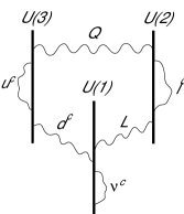
Figure 1: Pictorial representation of model A

and Fig. 2 (models B,C).

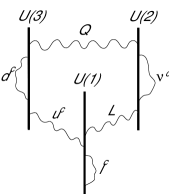
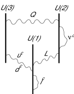
Figure 2: Pictorial representation of models B and C

Thus, the members of a family of quarks and leptons have the following quantum numbers:

$${\rm Model\ A}$$

$$\!\!\!\!\!\!\!\!Q ({\bf 3},{\bf 2};1,1,0)_{1/6}$$

$$\!\!\!\!\!\!\!\!u^{c} (\bar{\bf 3},{\bf 1};2,0,0)_{-2/3}$$

$$\!\!\!\!\!\!\!\!d^{c} (\bar{\bf 3},{\bf 1};-1,0,\varepsilon_{d})_{1/3}$$ (10)

$$\!\!\!\!\!\!\!\!L ({\bf 1},{\bf 2};0,-1,\varepsilon_{L})_{-1/2}$$

$$\!\!\!\!\!\!\!\!l^{c} ({\bf 1},{\bf 1};0,2,0)_{1}$$

$$\!\!\!\!\!\!\!\!\nu^{c} ({\bf 1},{\bf 1};0,0,2\varepsilon_{\nu})_{0}$$

$${\rm Model\ B}\qquad\qquad\quad\ {\rm Model\ C}$$

$$\!\!\!\!\!\!\!\!Q ({\bf 3},{\bf 2};1,\varepsilon_{Q},0)_{1/6}\qquad\,({\bf 3},{\bf 2};1,\varepsilon_{Q},0)_{1/6}$$

$$\!\!\!\!\!\!\!\!u^{c} (\bar{\bf 3},{\bf 1};-1,0,1)_{-2/3}\quad\ (\bar{\bf 3},{\bf 1};-1,0,1)_{-2/3}$$

$$\!\!\!\!\!\!\!\!d^{c} (\bar{\bf 3},{\bf 1};2,0,0)_{1/3}\qquad\ \ \,(\bar{\bf 3},{\bf 1};-1,0,-1)_{1/3}$$ (11)

$$\!\!\!\!\!\!\!\!L ({\bf 1},{\bf 2};0,\varepsilon_{L},1)_{-1/2}\quad\ \ \,({\bf 1},{\bf 2};0,\varepsilon_{L},1)_{-1/2}$$

$$\!\!\!\!\!\!\!\!l^{c} ({\bf 1},{\bf 1};0,0,-2)_{1}\qquad\ \ ({\bf 1},{\bf 1};0,0,-2)_{1}$$

$$\!\!\!\!\!\!\!\!\nu^{c} ({\bf 1},{\bf 1};0,2\varepsilon_{\nu},0)_{0}\qquad\ \,({\bf 1},{\bf 1};0,2\varepsilon_{\nu},0)_{0}$$

where the last three digits after the semi-column in the brackets are the charges under the three abelian factors $U(1)_{3}\times U(1)_{2}\times U(1)$, that we will call $Q_{3}$, $Q_{2}$ and $Q_{1}$ in the following, while the subscripts denote the corresponding hypercharges. The various sign ambiguities $\varepsilon_{i}=\pm 1$ are due to the fact that the corresponding abelian factor does not participate in the hypercharge combination (see below). In the last lines, we also give the quantum numbers of a possible right-handed neutrino in each of the three models. These are in fact all possible ways of embedding the SM spectrum in three sets of branes.

The hypercharge combination is:

$${\rm Model\ A}\quad\ : \quad Y=-{1\over 3}Q_{3}+{1\over 2}Q_{2}$$ (12)

$${\rm Model\ B,C} : \quad Y=\ \ \,{1\over 6}Q_{3}-{1\over 2}Q_{1}$$

leading to the following expressions for the weak angle:

$${\rm Model\ A} : \sin^{2}\theta_{W}={1\over 2+2\alpha_{2}/3\alpha_{3}}={3\over 8}\,{\bigg{|}}_{\alpha_{{}_{2}}=\alpha_{{}_{3}}}$$ (13)

$${\rm Model\ B,C} : \sin^{2}\theta_{W}={1\over 1+\alpha_{2}/2\alpha_{1}+\alpha_{2}/6\alpha_{3}}$$

$$\qquad\quad\ ={6\over 7+3\alpha_{2}/\alpha_{1}}\,{\bigg{|}}_{\alpha_{{}_{2}}=\alpha_{{}_{3}}}$$

In the second part of the above equalities, we used the unification relation $\alpha_{2}=\alpha_{3}$, that can be naturally imposed as described in the previous section. It follows that model A admits natural gauge coupling unification of strong and weak interactions, and predicts the correct value for $\sin^{2}\theta_{W}=3/8$ at the unification scale $M_{\rm GUT}$.

Besides the hypercharge combination, there are two additional $U(1)$’s. It is easy to check that one of the two can be identified with $B-L$. For instance, in model A choosing the signs $\varepsilon_{d}=\varepsilon_{L}=-\varepsilon_{\nu}=-\varepsilon_{H}=\varepsilon_{H^{\prime}}$, it is given by:

$$B-L=-{1\over 6}Q_{3}+{1\over 2}Q_{2}-{\varepsilon_{d}\over 2}Q_{1}\,.$$ (14)

Finally, the above spectrum can be easily implemented with a Higgs sector, since the Higgs field $H$ has the same quantum numbers as the lepton doublet or its complex conjugate:

$${\rm Model\ A}\qquad\qquad\quad\quad{\rm Model\ B,C}$$

$$\!\!\!\!\!\!\!\!H\ ({\bf 1},{\bf 2};0,-1,\varepsilon_{H})_{-1/2}\quad\ ({\bf 1},{\bf 2};0,\varepsilon_{H},1)_{-1/2}$$ (15)

$$\!\!\!\!\!\!\!\!H^{\prime} ({\bf 1},{\bf 2};0,1,\varepsilon_{H^{\prime}})_{1/2}\qquad\ \,({\bf 1},{\bf 2};0,\varepsilon_{H^{\prime}},-1)_{1/2}$$

6 Mass scales

6.1 String scale

To preserve gauge coupling unification, the compactification scale (actually the smallest, if there are several) must be of order of the unification scale $M_{\rm GUT}\simeq 10^{16}$ GeV. Above this energy, gauge interactions acquire a higher dimensional behavior. Moreover, to keep the theory weakly coupled, the string scale $M_{s}\equiv{\alpha^{\prime}}^{-1/2}$ should be close to the compactification scale and therefore to $M_{\rm GUT}$. On the other hand, as we discussed above, to ensure that corrections to the unification of gauge couplings are within 1%, the magnetic fields should be weak, $|H_{I}^{a}|\alpha^{\prime}\mathrel{\lower 2.5pt\vbox{\hbox{$<$}\hbox{$\sim$}}}0.1$. From the quantization condition (3), it follows that the string scale should be roughly a factor of 3 higher than the compactification scale,

$$M_{s}\simeq 3\,M_{\rm GUT}\,.$$ (16)

6.2 Scalar masses

The supersymmetry breaking scale $m_{0}$ is given by the heaviest charged scalar mass (5): $m_{0}^{2}\sim\delta H^{a}\equiv\sum_{I=1}^{3}\epsilon_{I}H_{I}^{a}$ on brane stacks, and $m_{0}^{2}\sim\delta H^{a}-\delta H^{b}$ on brane intersections. Here, $\epsilon_{I}$ are signs: two positive and one negative. Thus, even for strong magnetic fields, of order of the string scale, $m_{0}$ can be much smaller and corresponds to an arbitrary parameter. Although values much lower than $M_{\rm GUT}$ require an apparent fine tuning of radii, such a tuning is technically natural since the supersymmetric point $m_{0}=0$ is radiatively stable.

All scalar masses are of the order of the supersymmetry breaking scale $m_{0}$, which is assumed to be very high in split supersymmetry, except for those coming from supersymmetric sectors, which are vanishing to lowest order, such as the higgses. The latter are expected to acquire masses from one loop corrections, proportional to $m_{0}$ but suppressed by a loop factor. Note that off diagonal elements of the $2\times 2$ Higgs mass matrix, usually denoted by $B\mu$, should also be generated at the same order as the diagonal elements, in the absence of a Peccei-Quinn (PQ) symmetry. For high $m_{0}$, a fine tuning between $B\mu$ and the diagonal elements is then required to ensure a light Higgs.

6.3 Gaugino masses

It remains to discuss the corrections to gaugino and higgsino masses, $m_{1/2}$ and $\mu$, which are vanishing at the tree-level. In the absence of gravity, they are both protected by an R-symmetry. Actually, higgsino masses are protected in addition by a PQ symmetry which must be broken in order to generate a $B\mu$ mixing term in the Higgs mass matrix, as we argued above. Then, a $\mu$-term can be generated via $B\mu$, or directly using the PQ symmetry breaking, if R-symmetry is broken. Indeed, R-symmetry is in general broken in the gravitational sector by the gravitino mass $m_{3/2}$ and thus, in the presence of gravity, $m_{1/2}$ and $\mu$ are not anymore protected. Since supersymmetry breaking in the gravity sector is model dependent and brings more uncertainties, here we will assume that gravitational corrections are negligible. For instance, if supergravity breaking occurs via a Scherk-Schwarz compactification on an interval transverse to our braneworld Antoniadis:1998ki , using the usual $\mathbb{Z}_{2}$ fermion number in the bulk, the gravitino acquires Dirac mass together with its Kaluza-Klein modes and R-symmetry remains unbroken Antoniadis:2004dt . One can therefore discuss other sources of R-symmetry breaking within only global supersymmetry.

As discussed previously, supersymmmetry breaking via internal magnetic fields is described in the 4d effective field theory by vacuum expectation values (VEVs) of D-term auxiliaries for all magnetic $U(1)$’s. In the low energy limit, one has:

$$\langle D\rangle\simeq m_{0}^{2}\,,$$ (17)

and thus R-symmetry remains unbroken. However, it is broken by $\alpha^{\prime}$-string corrections, that modify for instance the gauge kinetic terms to the DBI form. In particular, gaugino masses can be induced by a dimension-seven effective operator which is the chiral F-term Antoniadis:2005sd :

$$F_{(0,3)}\int d^{2}\theta{\cal W}^{2}{\rm Tr}W^{2}\quad\Rightarrow\quad m_{1/2}\sim{m_{0}^{4}\over M_{s}^{3}}\,,$$ (18)

where ${\cal W}$ and $W$ denote the magnetic $U(1)$ and non-abelian gauge superfield, respectively. The coefficient $F_{(0,3)}$ is a moduli dependent function given by the topological partition function on a world-sheet with no handles and three boundaries. It is non-vanishing when the three brane stacks associated to the boundaries do not intersect at a point in any of the three internal torii. From the effective field theory point of view, it corresponds to a two-loop correction involving massive open string states. Upon a VEV $\langle{\cal W}\rangle=\theta\langle D\rangle$, the above F-term generates gaugino masses given in eq. (18). They are in the TeV region for scalar masses at intermediate energies, $m_{0}\sim{\cal O}(10^{13})$ GeV.

7 Split extended supersymmetry

Implementing split supersymmetry in string theory faces a generic problem: in simple brane constructions the gauge sector comes in multiplets of extended supersymmetry Blumenhagen:2005mu ; marc . ${\cal N}=4$ in the toroidal case, or ${\cal N}=2$ is simple orbifolds. Gauginos can therefore get Dirac masses without breaking R-symmetry. Indeed, a Dirac mass Fox:2002bu is induced through the dimension-five operator

$$\frac{a}{M_{s}}\int d^{2}\theta{\mathcal{W}}\,W^{a}A_{a}\ \Rightarrow m_{D}\sim a\frac{m_{0}^{2}}{M_{s}}\,,$$ (19)

where $a$ accounts for a possible loop factor. Actually, this operator arises quite generally at one-loop level in intersecting D-brane models with a moduli-dependent coupling, determined only from the massless (topological) sector of the theory marc . Note that this mass $m_{D}$ is much higher that the Majorana induced mass of eq. (18).

It turns out that this scenario is compatible with one-loop gauge coupling unification Antoniadis:2005em . In the energy regime between $M_{\rm GUT}$ and the electroweak scale $M_{W}$, the renormalization group equations meet three thresholds. From $M_{\rm GUT}$ to the common scalar mass $m_{0}$ all charged states contribute. Below $m_{0}$ squarks and sleptons (which do not affect unification), adjoint scalars and $2-n_{H}$ higgses decouple, while below $m_{D}$ the ${\cal N}=2$ or ${\cal N}=4$ gluinos and winos drop out. Finally, at TeV energies higgsinos decouple and we are left with the Standard Model with $n_{H}$ Higgs doublets. Using $M_{s}\sim M_{\rm GUT}$ and varying $a$ between $a=1$ and $a=1/100$, one finds realistic values for $M_{\rm GUT}$ and $m_{0}$ in both ${\cal N}=4$ and ${\cal N}=2$ cases. The results are summarized in Table 1.

	$n_{H}$	$M_{\rm GUT}$	$m_{0}$	$m_{D}$	$m_{1/2}$
${\cal N}=2$	$1$	$10^{18}$	$10^{13}$	$10^{6}$	$10^{-5}$
	$2$	$10^{16}$	$10^{13}$	$10^{9}$	$10^{2}$
${\cal N}=4$	$1$	$10^{19}$	$10^{16}$	$10^{12}$	$10^{6}$
	$2$	—	—	—	—

Table 1: Values for the unification scale $M_{\rm GUT}$, scalar masses $m_{0}$, Dirac gaugino masses $m_{D}$, and Majorana gaugino masses $m_{1/2}$ in GeV for ${\cal N}=2,4$ supersymmetric gauge sector and $n_{H}=1,2$ light higgses.

In all cases the unification scale is high enough to avoid problems with proton decay. For the two possible cases with one light Higgs (${\cal N}=2$ or ${\cal N}=4$), $M_{\rm GUT}$ is very close to the Planck scale so that there should be no need to explain the usual mismatch between these two scales.

The low energy sector of these models contains, besides the SM, just some fermion doublets (higgsinos) and eventually two singlets (the binos from the discussion below). It therefore illustrates the fact that only these states are needed for a minimal extension of the SM consistent with unification and Dark Matter (DM) candidates, and not the full fermion spectrum of split supersymmetry Arkani-Hamed:2005yv .

Another constraint on the models is that they must provide a DM candidate. As usually in supersymmetric theories this should be the lightest neutralino. Pure higgsinos cannot be DM candidates because their mass is of Dirac type. Since DM direct detection experiments have ruled out Dirac fermions up to masses of order $50$ TeV, some mixing coming from the binos is required in order to break the degeneracies of the two lightest neutralinos; the required mass difference is bigger than about 150 keV Smith:2001hy ; Giudice:2004tc ; Antoniadis:2005em . This translates into an upper bound on the Dirac gaugino mass of about $10^{5}$ GeV, for the required higgsino mass splitting to be generated through the electroweak symmetry breaking mixing, which is of order $m_{W}^{2}/m_{D}$. This value compared to the values in Table 1 leads to the ${\cal N}=2$, $n_{H}=1$ case as the only possibility to accommodate it (the direct Majorana component of bino $m_{1/2}$ is negligible in this case). In fact, one needs an order of magnitude suppression of the induced Dirac mass for binos relative to the other gauginos, which is not unreasonable to assume in brane constructions.

In the other two models, the required suppression factor is much higher and the above mechanism would be very unnatural. However, since binos play no role for unification as they carry no SM charge, we could imagine a scenario where $m_{D}$ vanishes identically for binos, but not for the other gauginos. For instance consider the case where Dirac masses from the operator (19) are generated by loop diagrams involving ${\cal N}=2$ hypermultiplets with supersymmetric masses of order $M_{\rm GUT}$ and a supersymmetry breaking splitting of order $m_{0}$. It is then possible to choose these massive states such that they carry no hypercharge, in which case binos can only have Majorana masses displayed in Table 1. Their value in the ${\cal N}=4$ case corresponds to the upper bound for DM with Majorana bino mass Antoniadis:2005em . Thus, the constraint of a viable DM candidate leaves us with two possibilities: (a) ${\cal N}=2$ with $n_{H}=1$ and Dirac masses for all gauginos and (b) ${\cal N}=4$ with $n_{H}=1$, or ${\cal N}=2$ with $n_{H}=2$ and Majorana mass binos.

Finally, the higgsinos must acquire a mass of order the electroweak scale. This can be induced by the following dimension-seven operator, generated at one loop level Antoniadis:2005sd ; marc :

$$\frac{c}{M_{s}^{3}}\int d^{2}\theta\mathcal{W}^{2}\overline{D}^{2}{\bar{H}}_{1}{\bar{H}}_{2}\Rightarrow\mu\sim c\frac{m_{0}^{4}}{M_{s}^{3}}\,,$$ (20)

where $c$ is again a loop factor. The resulting numerical value is of the same order as $m_{1/2}$. Thus, such an operator can only give a sensible value of $\mu$ for the ${\cal N}=2$ $n_{H}=2$ model. In the other two cases, ${\cal N}=4$ or ${\cal N}=2$ with $n_{H}=1$, $\mu$ remains an independent parameter.

To summarize, at low energies we end up with two distinct scenarios after all massive particles are decoupled: (i) $n_{H}=1$ with light higgsinos (models with ${\cal N}=2$ and ${\cal N}=4$ gauge sector and $n_{H}=1$), and (ii) $n_{H}=2$ with light higgsinos and binos (model with ${\cal N}=2$ gauge sector and $n_{H}=2$). In the $n_{H}=1$ scenario the DM candidate is mainly higgsino, although the much heavier bino is light enough to forbid any vector couplings. The relic density reproduces the actual WMAP results for $\mu\sim 1.1$ TeV.

References

- (1) N. Arkani-Hamed and S. Dimopoulos, arXiv:hep-th/0405159.
- (2) G. F. Giudice and A. Romanino, Nucl. Phys. B 699, 65 (2004) [Erratum-ibid. B 706, 65 (2005)] [arXiv:hep-ph/0406088].
- (3) I. Antoniadis and S. Dimopoulos, Nucl. Phys. B 715, 120 (2005) [arXiv:hep-th/0411032].
- (4) I. Antoniadis, K. S. Narain and T. R. Taylor, arXiv:hep-th/0507244.
- (5) I. Antoniadis, A. Delgado, K. Benakli, M. Quiros and M. Tuckmantel, arXiv:hep-ph/0507192.
- (6) I. Antoniadis, Phys. Lett. B 246 (1990) 377; J. D. Lykken, Phys. Rev. D 54 (1996) 3693 [arXiv:hep-th/9603133].
- (7) N. Arkani-Hamed, S. Dimopoulos and G. R. Dvali, Phys. Lett. B 429 (1998) 263 [arXiv:hep-ph/9803315]; I. Antoniadis, N. Arkani-Hamed, S. Dimopoulos and G. R. Dvali, Phys. Lett. B 436 (1998) 257 [arXiv:hep-ph/9804398].
- (8) C. Angelantonj and A. Sagnotti, Phys. Rept. 371 (2002) 1 [Erratum-ibid. 376 (2003) 339] [arXiv:hep-th/0204089].
- (9) C. Bachas, arXiv:hep-th/9503030.
- (10) C. Angelantonj, I. Antoniadis, E. Dudas and A. Sagnotti, Phys. Lett. B 489 (2000) 223 [arXiv:hep-th/0007090].
- (11) M. Berkooz, M. R. Douglas and R. G. Leigh, Nucl. Phys. B 480 (1996) 265 [arXiv:hep-th/9606139];
- (12) R. Blumenhagen, L. Goerlich, B. Kors and D. Lust, JHEP 0010 (2000) 006 [arXiv:hep-th/0007024]; G. Aldazabal, S. Franco, L. E. Ibanez, R. Rabadan and A. M. Uranga, J. Math. Phys. 42 (2001) 3103 [arXiv:hep-th/0011073].
- (13) R. Blumenhagen, D. Lust and S. Stieberger, JHEP 0307 (2003) 036 [arXiv:hep-th/0305146].
- (14) I. Antoniadis, E. Kiritsis and T. N. Tomaras, Phys. Lett. B 486 (2000) 186 [arXiv:hep-ph/0004214]; I. Antoniadis, E. Kiritsis, J. Rizos and T. N. Tomaras, Nucl. Phys. B 660 (2003) 81 [arXiv:hep-th/0210263]; R. Blumenhagen, B. Kors, D. Lust and T. Ott, Nucl. Phys. B 616, 3 (2001) [arXiv:hep-th/0107138]; I. Antoniadis and J. Rizos, 2003 unpublished work.
- (15) I. Antoniadis, E. Dudas and A. Sagnotti, Nucl. Phys. B 544 (1999) 469 [arXiv:hep-th/9807011].
- (16) For a recent review, see R. Blumenhagen, M. Cvetic, P. Langacker and G. Shiu, arXiv:hep-th/0502005; and references therein.
- (17) I. Antoniadis, K. Benakli, A. Delgado, M. Quirós and M. Tuckmantel, to appear.
- (18) P. J. Fox, A. E. Nelson and N. Weiner, JHEP 0208 (2002) 035 [arXiv:hep-ph/0206096].
- (19) N. Arkani-Hamed, S. Dimopoulos and S. Kachru, arXiv:hep-th/0501082.
- (20) D. R. Smith and N. Weiner, Phys. Rev. D 64 (2001) 043502 [arXiv:hep-ph/0101138].