On singular effective superpotentials in supersymmetric gauge theories

Abstract:

We study $N=1$ supersymmetric $\mathop{\rm SU}(2)$ gauge theory in four dimensions with a large number of massless quarks. We argue that effective superpotentials as a function of local gauge-invariant chiral fields should exist for these theories. We show that although the superpotentials are singular, they nevertheless correctly describe the moduli space of vacua, are consistent under RG flow to fewer flavors upon turning on masses, and also reproduce by a tree-level calculation the higher-derivative F-terms calculated by Beasely and Witten [1] using instanton methods. We note that this phenomenon can also occur in supersymmetric gauge theories in various dimensions.

1 Introduction and summary

Using the selection rules of four dimensional $N=1$ supersymmetry, exact results for superpotentials for supersymmetric gauge theories have been obtained; see [2, 3] for short reviews. These results have been inferred in field theory by an elaborate series of consistency checks, having largely to do with consistency upon integrating out massive chiral multiplets. The basic strategy for finding these results has been a loose kind of induction in the number of light flavors in which one works one’s way up to larger numbers of light flavors by making consistent guesses. The heuristic picture obtained in this way for superQCD is that quantum effects are more pronounced in the low energy effective action the fewer the number of light flavors.

It is natural to ask whether this procedure can be made more deductive and uniform by turning it on its head, and starting instead with the IR free theories with many massless flavors. Since the leading low energy effective action of IR free theories are free, how do they manage to generate the strong quantum effects as flavors are integrated out? Recently, C. Beasely and E. Witten [1] have shed light on how quantum effects at low number of flavors are inherited from the large-flavor theory. They found that at large number of flavors there are higher-derivative $F$-terms (of a special form) in the action which, upon integrating out, descend to lower-derivative operators, until they finally become relevant, and manifest themselves as quantum corrections in the low energy effective action (e.g. as a quantum deformation of the moduli space).

They compute these terms in $\mathop{\rm SU}(2)$ superQCD with an arbitrary number ${n_{f}}$ of fundamental flavors by a one-instanton argument. This is done intrinsically on the moduli space, i.e. using only the massless multiplets in the vicinity of an arbitrary non-singular point on the moduli space. But, interestingly, for ${n_{f}}=2$ and $3$ they also show that the higher-derivative terms can be derived by simply integrating out massive modes at tree-level from an effective superpotential defined on a larger configuration space made up of vevs of the local gauge-invariant chiral meson field.

This raises the question of whether a similar efficient description of larger-flavor cases can be made in terms of effective superpotentials. Now, such superpotentials are thought to be problematic because, for large enough number of flavors, they are singular [4, 5] when expressed in terms of local gauge-invariant chiral vevs, even away from the origin. Also, these superpotentials do not vanish as the strong-coupling scale of the theory $\Lambda$ vanishes. Indeed, such an effective superpotential need not even exist [4]; for only if there is a region in the configuration space of the chosen chiral vevs where all of them are light together and comprise all the light degrees of freedom, are we then assured that there is a Wilsonian effective action in terms of these fields in that region. If this condition is satisfied, then the resulting effective superpotential can be extended over the whole configuration space by analytic continuation using the holomorphy of the superpotential. For large-flavor superQCD, the only region where all the components of the meson and baryon fields become light at the same time is at the origin. But ’t Hooft anomaly matching conditions imply [6] that there must be additional extra light degrees of freedom beyond the meson and baryon fields at the origin. Thus no superpotential written solely in terms of mesons and baryons need exist, for there is no guarantee that modes of other operators which account for the additional massless degrees of freedom at the origin are not as light as the meson and baryon modes, and so must also be included in a consistent effective action.

However, when there are so many massless flavors that the theory is IR free, we know what the light degrees of freedom are near the origin, since we have a weakly coupled lagrangian description there. The physics can be made arbitrarily weakly coupled simply by taking all scalar field vevs $\mu\sim\langle\phi\rangle<<\Lambda$ where $\Lambda$ is the strong coupling scale (or UV cutoff) of the IR free theory. In this limit the physics is just the classical Higgs mechanism, and all particles get masses of order $\mu$ or less. The Wilsonian effective description results from integrating out modes with energies greater than a cutoff, which we take to be some multiple of $\mu$. The effective action will then include all local gauge-invariant operators made from the fundamental fields in the lagrangian and which can create particle states with masses below the cutoff. For the purpose of constructing the effective superpotential, the relevant local gauge-invariant operators are those in the chiral ring. It is then just a matter of constructing a set of operators in the classical gauge theory which generates the chiral ring. An effective superpotential which is a function of these operators must then exist.

To be concrete, consider the simplest example, which will be the focus of this paper: $N=1$ supersymmetric $\mathop{\rm SU}(2)$ QCD in four dimensions. This theory has an adjoint vector “gluon” multiplet $W^{(ab)}_{\alpha}$ and $2{n_{f}}$ fundamental “quark” chiral multiplets $Q^{i}_{a}$; $a,b$ are $\mathop{\rm SU}(2)$ color indices. One can show [7, 8] that a complete basis of local gauge-invariant operators in the chiral ring in this theory is comprised of just the glueball $S\sim W_{\alpha}\cdot W^{\alpha}$ and the meson operators $M^{ij}\sim Q^{i}\cdot Q^{j}$. At a suitably symmetric vacuum, say $\langle Q^{i}_{a}\rangle=\mu\delta^{i}_{a}$, the gauge bosons and the quarks $Q^{i}_{a}$ with $i>2$, as well as their superpartners, all get mass $\mu$ by the Higgs mechanism. So, since the glueball and meson operators only involve the product of two fundamental fields, they create modes of particle states with mass at most $2\mu$. (The masses just add since, by taking $\mu<<\Lambda$, we are at arbitrarily weak coupling.) Thus in a Wilsonian effective action found by integrating out modes above $2\mu$ we may consistently keep all components of $S$ and $M^{ij}$, and since they generate the chiral ring, there must exist an effective superpotential which is a function of only these chiral fields.

So far we have argued that an effective superpotential for local gauge-invariant operators in the chiral ring exists and makes sense for superQCD with enough massless flavors that it is IR free. This does not show the existence of such an effective superpotential in the asymptotically free case. In particular, for theories in the “conformal window” where neither the direct nor Seiberg dual description is IR free [6] (e.g. $3<{n_{f}}<6$ for $\mathop{\rm SU}(2)$ gauge group), we have no useful description of the light degrees of freedom at the origin of moduli space. Nevertheless, given an effective superpotential for an IR free theory, we can always integrate out flavors using holomorphy to derive consistent effective superpotentials in the conformal window. This round-about argument assures us that effective superpotentials exist for all numbers of light flavors in superQCD.

1.1 Outline of the paper

In this paper we illustrate this line of reasoning for the simplest example: four-dimensional $N=1$ supersymmetric $\mathop{\rm SU}(2)$ QCD with many light fundamental flavors. The form of the effective superpotential is fixed by the global symmetries, making this a particularly easy case to study.

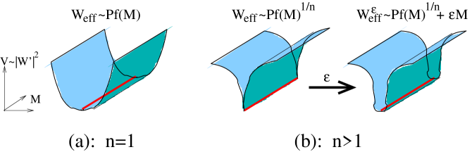
Figure 1: Sketches of the effective potential as a function of the meson vevs for $\mathop{\rm SU}(2)$ superQCD with (a) $n:={n_{f}}-2=1$, where the potential is regular, and (b) for $n>1$, where the potential has a cusp but can be smoothed by a small perturbation $\varepsilon$. Red lines denote the moduli spaces (vacua).

We start in section 2 by assuming we can integrate out the glueball degrees of freedom to express the superpotential solely in terms of the meson vevs. The resulting superpotentials, determined by the symmetries, are singular. We show that they are, nevertheless, perfectly sensible. The cusp-like behavior of their associated potentials still unambiguously describes their supersymmetric minima. They can be regularized by turning on arbitrarily small quark masses. We then observe that no matter how the masses are sent to zero, these superpotentials always give the correct constraint equation describing the moduli space. The basic point is illustrated in figure 1: even though the potential has cusp-like singularities all along the moduli space, it nevertheless has a well-defined minimum. We also show that upon giving large masses to some flavors and integrating them out, we recover the superpotential for fewer numbers of flavors.

In section 3 we justify the assumption that the glueball field can be consistently integrated out. Using the Konishi anomaly [9, 10], one can derive a partial differential equation satisfied by the superpotential as a function of the meson and glueball vevs. We solve these equations, determining the integration function by matching to the Veneziano-Yankielowicz superpotential [11] for pure $\mathop{\rm SU}(2)$ superYang-Mills. Since in the IR free case we have included all the local chiral light degrees of freedom, by the arguments of this section we expect these differential equations to be integrable and the superpotential to exist. Indeed they are and it does, and matches (upon integrating out the glueballs) the results of section 2.

In the asymptotically free cases in the conformal window, $3<{n_{f}}<6$, since there is no argument that it is consistent to describe the effective theory in terms of the local gauge-invariant chiral ring made from the microscopic fields, it is possible that the differential equations for the effective superpotential derived from the Konishi anomaly may not be integrable. In the case of $\mathop{\rm SU}(2)$ superQCD, however, we find that they are integrable. This is presumably an “accident” due to the large global symmetry group of the theory, and need not remain the case for $\mathop{\rm SU}({n_{c}})$ with ${n_{c}}>2$ [12]. We also check that we get the same superpotential by using the Konishi anomaly equation in both the direct and Seiberg dual description of the low energy theory.

We justified the existence of these singular effective superpotentials in IR free theories. By integrating out flavors we can use them to deduce the correct effective superpotentials for few numbers of flavors where quantum effects dramatically alter the form of the superpotential (first deforming the classical moduli space, then lifting it altogether as flavors are integrated out). It was shown in [1] that in a description in terms of only the massless multiplets in the vicinity of an arbitrary non-singular point on the moduli space, these strong quantum effects descend from higher-derivative F-terms which can be calculated using instanton methods. It is therefore a non-trivial, and quite elaborate, check of our singular superpotentials that by expanding them around a generic vacuum and integrating out at tree level the massive modes of the meson field (those that take us off the moduli space), we reproduce the higher-derivative F-terms computed in [1]. We perform this check in section 4.

Singular superpotentials are a generic feature of gauge theories with a large number of flavors, and are not special just to four-dimensional theories. In section 5 we argue in an example with three-dimensional $N=2$ supersymmetry where the global symmetries are enough to fix a singular form for the effective superpotential, that these superpotentials satisfy a similar set of consistency checks as do the four-dimensional theories. However, in this case we no longer have an IR free regime as a starting point from which to derive effective superpotentials by integrating out flavors using holomorphy. Thus the meaning of singular effective superpotentials is less certain in $d<4$.

2 Effective superpotentials for SU(2) superQCD with $\bf{n_{f}}>3$

$N=1$ supersymmetric $\mathop{\rm SU}(2)$ QCD has an adjoint vector multiplet $W^{(ab)}_{\alpha}$ containing the gluons and $2{n_{f}}$ massless quark chiral multiplets $Q^{i}_{a}$ in the fundamental representation; $i,j=1,\ldots,2{n_{f}}$ are flavor indices and $a,b=1,2$ are $\mathop{\rm SU}(2)$ color indices. (There must be an even number of flavors for anomaly cancellation [13].) The classical moduli space of vacua is conveniently parametrized in terms of the vevs of the antisymmetric, gauge-singlet chiral meson fields $\hat{M}^{[ij]}:=Q^{i}_{a}\epsilon^{ab}Q^{j}_{b}$, where $\epsilon^{ab}$ is the invariant antisymmetric tensor of $\mathop{\rm SU}(2)$. For ${n_{f}}=1$ the classical moduli space is the space of arbitrary meson vevs $M^{ij}$, while for ${n_{f}}\geq 2$ it is all $M^{ij}$ satisfying the constraint

$$\epsilon_{i_{1}\cdots i_{2{n_{f}}}}M^{i_{1}i_{2}}M^{i_{3}i_{4}}=0,$$ (1)

or, equivalently, rank$(M)\leq 2$.

The moduli space is modified by quantum effects when ${n_{f}}<3$. For ${n_{f}}=1$, there is a dynamically generated superpotential which lifts all the classical flat directions [14],

$${W_{\rm eff}}={\Lambda^{5}\over\mbox{Pf}\,M},\qquad\qquad\qquad({n_{f}}=1)$$ (2)

where $\Lambda$ is the strong-coupling scale of the theory and the Pfaffian is defined as $\mbox{Pf}\,M:=\epsilon_{i_{1}\cdots i_{2{n_{f}}}}M^{i_{1}i_{2}}\cdots M^{i_{2{n_{f}}-1}i_{2{n_{f}}}}=\sqrt{\mbox{det}\,M}$. For ${n_{f}}=2$ the superpotential can be written [4]

$${W_{\rm eff}}=\Sigma\left(\mbox{Pf}\,M-\Lambda^{4}\right),\qquad({n_{f}}=2)$$ (3)

where $\Sigma$ is a Lagrange multiplier enforcing a quantum-deformed constraint $\mbox{Pf}\,M=\Lambda^{4}$, which removes the singularity at the origin of the classical moduli space.

For ${n_{f}}=3$ the superpotential is [4]

$${W_{\rm eff}}=-{1\over\Lambda^{3}}\mbox{Pf}\,M.\qquad\qquad({n_{f}}=3)$$ (4)

The resulting equations of motion reproduce the classical constraint (1), which are therefore not modified quantum mechanically. Note that although the superpotential (4) apparently diverges in the weak-coupling $\Lambda\to 0$ limit, it actually vanishes on the moduli space since (1) implies $\mbox{Pf}\,M=0$. The negative power of $\Lambda$ reflects the fact that fluctuations off the classical constraint surface become infinitely massive in the weak coupling limit.

2.1 Singular superpotential for $\bf{n_{f}}>3$ and the classical constraints

For ${n_{f}}>3$, the classical constraints are also not modified quantum mechanically. However, the complex singularities of the moduli space defined by (1) indicate the presence of new massless degrees of freedom there, in addition to the components of $\hat{M}^{ij}$ [6].

We argued in section 1 that, nevertheless, an effective superpotential for the IR free case (${n_{f}}>5$) should exist as a function of the unconstrained chiral meson and glueball vevs, $M^{ij}$ and $S$. For the moment, let us assume that the glueball superfield can always be conistently integrated out away from the origin, so we can just deal with an effective superpotential depending only on $M^{ij}$. Then the possible form of the effective superpotential is completely determined by the symmetries up to an overall numerical factor.

The only effective superpotential consistent with holomorphicity, weak-coupling limits, and the global symmetries is [5]

$${W_{\rm eff}}=-n\left(\mbox{Pf}\,M\over\Lambda^{b_{0}}\right)^{1/n},\qquad n:={n_{f}}-2>1$$ (5)

where $b_{0}=6-{n_{f}}$ is the coefficient of the one-loop beta function. The coefficient in (5) will be justified below. We will also check below that this superpotential is consistent under integrating out successive flavors, and so its form in the asymptotically free cases (${n_{f}}<6$) follow from any IR free case (${n_{f}}\geq 6$) by holomorphy and RG flow. We leave the justification of the assumption that $S$ can be integrated out to section 3.

The fractional power of $\mbox{Pf}\,M$ in (5) implies that this superpotential has a cusp-like singularity at its extrema. The rest of this paper is devoted to arguing that this superpotential is nevertheless correct.

The first issue is how the classical constraint (1) follows from extremizing (5). Because these superpotentials are singular at their extrema, we cannot just take derivatives. Instead, we deform ${W_{\rm eff}}$ by introducing regularizing parameters before extremizing. Independent of how the regularizing parameters are sent to zero, the extrema of the superpotential will give the classical constraints (1).

We regularize (5) by adding a mass term with an invertible antisymmetric mass matrix $\varepsilon_{ij}$ for the meson fields,

$${W^{\varepsilon}_{\rm eff}}:={W_{\rm eff}}+{1\over 2}\varepsilon_{ij}M^{ij}.$$ (6)

We regularize ${W_{\rm eff}}$ with a term linear in $M$ since that is the only integral power of $M$ that smoothes the minima but is subleading at large $M$, and therefore does not create spurious extrema. Varying ${W^{\varepsilon}_{\rm eff}}$ with respect to $M^{kl}$ yields the equation of motion

$$M^{kl}=-\Lambda^{-b_{0}/n}(\mbox{Pf}\,M)^{1/n}(\varepsilon^{-1})^{kl}.$$ (7)

Solving for $\mbox{Pf}\,M$ in terms of $\varepsilon$ and substituting back gives $M^{kl}=-\Lambda^{b_{0}/2}(\mbox{Pf}\,\varepsilon)^{1/2}(\varepsilon^{-1})^{kl}$ which in turn implies

$$\epsilon_{i_{1}\ldots i_{2{n_{f}}}}M^{i_{1}i_{2}}M^{i_{3}i_{4}}={1\over\Lambda^{b_{0}}}\epsilon_{i_{1}\ldots i_{2{n_{f}}}}(\varepsilon^{-1})^{i_{1}i_{2}}(\varepsilon^{-1})^{i_{3}i_{4}}\ \mbox{Pf}\,\varepsilon.$$ (8)

The right hand side of the above expression is a polynomial of order $n>0$ in the $\varepsilon_{ij}$. Therefore, no matter how we send $\varepsilon_{ij}\to 0$, the right hand side will vanish, giving back the classical constraint (1). Furthermore, it is easy to check that any solution of the classical constraint can be reached in this way.

It may be helpful to present another, less formal, way of seeing how the classical constraint emerges from the singular effective superpotential. Use the global symmetry to rotate the meson fields into the skew diagonal form

$$M^{ij} = \pmatrix{M_{1}&&&\cr\ &M_{2}&&\cr\ &&\ddots&\cr\ &&&M_{{n_{f}}}\cr}\otimes i\sigma_{2},$$ (9)

so the effective superpotential (5) becomes

$${W_{\rm eff}}=-n\Lambda^{-b_{0}/n}\left(\prod_{i}M_{i}\right)^{1/n}.$$ (10)

The equations of motion which follow from extremizing with respect to the $M_{i}$ are

$$M_{i}^{{1\over n}-1}\prod_{j\neq i}M_{j}^{1\over n}=0.$$ (11)

Though these equations are ill-defined if we set any of the $M_{i}=0$, we can probe the solutions by taking limits as some of the $M_{i}$ approach zero. To test whether there is a limiting solution where $K$ of the $M_{i}$ vanish, consider the limit $\varepsilon\to 0$ with $M_{1}\sim\varepsilon^{\alpha_{1}},\ldots,M_{K}\sim\varepsilon^{\alpha_{K}}$ with $\alpha_{j}>0$ to be determined. Plugging into (11), only the first $K$ equations have non-trivial limits

$$\lim_{\varepsilon\to 0}\varepsilon^{{1\over n}\left(\sum_{j}\alpha_{j}\right)-\alpha_{i}}=0,\qquad i=1,\ldots,K,$$ (12)

giving the system of inequalities $n\alpha_{i}<\sum_{j}\alpha_{j}$ for $i=1,\ldots,K$. These inequalities have solutions if and only if $K>n$, implying that rank$(M)\leq 2$ which is precisely the classical constraint (1).

Note that, as in the ${n_{f}}=3$ case discussed above, the negative power of $\Lambda$ appearing in the effective superpotential (5) is not inconsistent with the weak coupling limit because the equations of motion (1) following from the superpotential imply $\mbox{Pf}\,M=0$, so that (5) vanishes on the moduli space.

2.2 Consistency upon integrating out flavors

Besides correctly describing the moduli space, the effective superpotentials should also pass some other tests. If we add a mass term for one flavor in the superpotential of a theory with ${n_{f}}$ flavors and then integrate it out, we should recover the superpotential of the theory with ${n_{f}}-1$ flavors. To show that the effective superpotential (5) passes this test, we add a gauge-invariant mass term for one flavor, say $M^{{2{n_{f}}-1}~{}{2{n_{f}}}}$,

$${W_{\rm eff}}=-n\Lambda^{-b_{0}/n}(\mbox{Pf}\,M)^{1/n}+mM^{{2{n_{f}}-1}~{}{2{n_{f}}}}.$$ (13)

The equations of motion for $M^{{i}~{}{2{n_{f}}-1}}$ and $M^{{j}~{}{2{n_{f}}}}$ (for $i\neq 2{n_{f}}-1$ and $j\neq 2{n_{f}}$) put the meson matrix into the form $M^{ij}={\widehat{M}\ 0\choose 0\ \widehat{X}}$ where $\widehat{M}$ is a $2({n_{f}}-1)\times 2({n_{f}}-1)$ and $\widehat{X}$ a $2\times 2$ matrix. Integrating out $\widehat{X}\sim M^{{2{n_{f}}-1}~{}{2{n_{f}}}}\otimes\sigma_{2}$ by its equation of motion gives

$${W_{\rm eff}}=-(n-1)\widehat{\Lambda}^{b_{0}/(n-1)}(\mbox{Pf}\,\widehat{M})^{1/(n-1)},$$ (14)

where $\widehat{\Lambda}=m\Lambda^{6-{n_{f}}}$ is the strong-coupling scale of the theory with ${n_{f}}-1$ flavors, consistent with matching the RG flow of the couplings at the scale $m$. Dropping the hats, we recognize (14) as the effective superpotentials of $\mathop{\rm SU}(2)$ superQCD with ${n_{f}}-1$ flavors.

3 Consistency with the Konishi anomaly equation

The Konishi anomaly implies a differential equation which the effective superpotential should obey when considered as a function of the meson and glueball vevs. We outline here the derivation of this equation and show that its solution enables us to determine the dependence of the effective superpotential on the glueball vev, and to justify the assumption that made in section 2 that the glueball superfield can be consistently integrated out. Although this is a simple exercise, it gains interest when compared to the $\mathop{\rm SU}(N)$ case where the corresponding generalized Konishi anomaly equations [7] are much more complicated [15, 12], as mentioned in section 1.

In the chiral ring the Konishi anomaly [9, 10] for a tree level superpotential $W_{\rm tree}$ takes the form

$$\langle{{\partial}W_{\rm tree}\over{\partial}Q_{a}^{i}}Q_{a}^{j}\rangle=S\delta^{j}_{i}.$$ (15)

where $S$ is the vev of the glueball superfield $\hat{S}={1\over{32\pi^{2}}}\mathop{\rm tr}({W^{\alpha}W_{\alpha}})$. (We distinguish an operator from its vev by putting a hat on the operator.) This is a special case of the generalized Konishi anomaly, which is perturbatively one-loop exact [7], and has also been shown [17] to be non-perturbatively exact for a $\mathop{\rm U}(N)$ gauge theory with matter in the adjoint representation as well as for $\mathop{\rm Sp}(N)$ and $\mathop{\rm SO}(N)$ gauge theories with matter in symmetric or antisymmetric representations. For the theory we are discussing here, we will not prove that the Konishi anomaly is non-perturbatively exact, though presumably this can be done along the lines of [17]. Instead, because the global symmetry of the $\mathop{\rm SU}(2)$ superQCD uniquely determines the superpotential as discussed in the previous section, we only need check that the Konishi anomaly equation implies this form of the superpotential. This check serves as evidence for the non-perturbative exactness of the Konishi anomaly equation for the theory under discussion. Had the Konishi anomaly equation been modified non-perturbatively, we would have found a different result for ${W_{\rm eff}}$ in this section.

3.1 Direct description

In the Konishi anomaly equation (15), take as our tree level superpotential

$$W_{\rm tree}=m_{ij}(\hat{M}^{ij}-M^{ij}),$$ (16)

so that

$$m_{ij}=-{1\over 2}{{{\partial}{W_{\rm eff}}}\over{\partial}M^{ij}},$$ (17)

is a Lagrange multiplier imposing that $M^{ij}$ are the vacuum expectation values of the meson operators $\hat{M}^{ij}$. Substituting (16) into (15) and using the fact that the expectation value of a product of gauge-invariant chiral operators equals the product of the expectation values of the individual ones, gives $2m_{ik}M^{kj}=S\delta^{j}_{i}$. Using (17) we then obtain a partial differential equation for the effective superpotential,

$${{\partial}{W_{\rm eff}}\over{\partial}M^{ik}}M^{kj}=S\delta^{j}_{i},$$ (18)

whose solution is

$${W_{\rm eff}}(M,S)=S\ln\left(\mbox{Pf}\,M\over\Lambda^{2{n_{f}}}\right)+f(S),$$ (19)

where $f(S)$ is an undetermined function. Upon giving the quarks a mass $m$ and integrating them out, the superpotential reduces to $f(S)+{n_{f}}S[\ln S-\ln(m\Lambda^{2})-1]$. In the limit $m\to\infty$, $\Lambda\to 0$ keeping $\Lambda_{0}$ fixed, where $6\ln\Lambda_{0}=b_{0}\ln\Lambda+{n_{f}}\ln m$, this becomes the $\mathop{\rm SU}(2)$ superYang-Mills theory with strong coupling scale $\Lambda_{0}$. The superpotential for this theory is the Veneziano-Yankielowicz superpotential [11] $W_{\rm VY}(S)=2S\left[\ln(S/\Lambda_{0}^{3})-1\right]$, implying that

$$f(S)=(2-{n_{f}})S\left[\ln(S/\Lambda^{3})-1\right].$$ (20)

Substituting (20) into (19) gives the effective superpotential as a function of $S$ and $M^{ij}$. It is easy to see that at its extrema $S$ is massive (except at the origin), justifying the assumption of the last section that it could be integrated out. Finally, integrating $S$ out by solving its equation of motion, we arrive at the effective superpotential (5).

3.2 Seiberg dual description

Viewing our $\mathop{\rm SU}(2)$ theory as an $\mathop{\rm Sp}(1)$ gauge theory, when ${n_{f}}>3$ the theory has a Seiberg dual description [5] in terms of an $\mathop{\rm Sp}({n_{f}}-3)$ gauge group. The dual $\mathop{\rm Sp}({n_{f}}-3)$ theory has $2{n_{f}}$ dual quark chiral multiplets $q^{a}_{i}$ in the fundamental representation as well as a gauge-singlet chiral multiplet $\hat{\cal M}^{[ij]}$ which is coupled to the dual meson fields $\hat{\cal N}_{ij}:=q^{a}_{i}J_{ab}q^{b}_{j}$ through the superpotential $W=\hat{\cal N}_{ij}\hat{\cal M}^{ij}$. Here $J_{ab}$ is the invariant symplectic antisymmetric tensor, $i,j=1,\ldots,2{n_{f}}$ are flavor indices, and $a,b=1,\ldots,2{n_{f}}-6$ are the gauge indices. This superpotential gives masses to the dual quarks and sets ${\cal N}_{ij}=0$ when ${\cal M}^{ij}\neq 0$. The dual description is IR free when ${n_{f}}<6$.

To determine the effective superpotentials of the dual theory we can either use the global symmetry, weak-coupling limit and the holomorphicity argument, or the Konishi anomaly equations. Both give the same answer; we discuss the Konishi anomaly equations. The ring of local gauge-invariant chiral operators is generated by $\hat{\SS}$, $\hat{\cal M}^{ij}$ and $\hat{\cal N}_{ij}$ [16]. The Konishi anomaly equations are $\langle q^{a}_{j}({\partial}W_{\rm tree}/{\partial}q^{a}_{i})\rangle=\SS\delta^{i}_{j}$. Take as the tree level superpotential

$$W_{\rm tree}=\hat{\cal N}_{ij}\hat{\cal M}^{ij}+m_{ij}(\hat{\cal M}^{ij}-{\cal M}^{ij}),$$ (21)

so that as before, $m_{ij}=-{1\over 2}({\partial}{W_{\rm eff}}/{\partial}{\cal M}^{ij})$, is a Lagrange multiplier imposing that ${\cal M}^{ij}$ are the vacuum expectation values of the scalar operators $\hat{\cal M}^{ij}$. We have not included a Lagrange multiplier for the dual mesons $\hat{\cal N}_{ij}$ because our analysis is valid only for points away from the origin of the moduli space where the dual quarks are massive.

As in the direct description, the Konishi anomaly with (21) gives $2{\cal M}^{ik}{\cal N}_{kj}=-\SS\delta^{i}_{j}$. The $\hat{\cal M}^{ij}$ equation of motion gives ${\cal N}_{ij}=-m_{ij}$, giving the partial differential equation ${\cal M}^{ik}({\partial}{W_{\rm eff}}/{\partial}{\cal M}^{kj})=\SS\delta^{i}_{j}$ whose solution is

$${W_{\rm eff}}({\cal M},\SS)=\SS\ln\left[{\mbox{Pf}\,{\cal M}\over\tilde{\Lambda}^{{n_{f}}}}\right]+f(\SS).$$ (22)

$f(\SS)$ is determined as before to be $f(\SS)=(2-{n_{f}})\SS[\ln(\SS/\tilde{\Lambda}^{3})-1]$. Integrating out $\SS$ then gives the effective superpotential in the dual description

$${W_{\rm eff}}=({n_{f}}-2){\left(\tilde{\Lambda}^{2{n_{f}}-6}\mbox{Pf}\,{\cal M}\right)}^{1\over{{n_{f}}-2}}.$$ (23)

The dual and direct descriptions are equivalent in the IR; the ${\cal M}^{ij}$ are identified with the direct theory mesons by ${\cal M}^{ij}={1\over\mu}M^{ij}$, where $\mu$ is a mass scale related to the dual and the direct theory strong-coupling scales by [5]

$$\Lambda^{6-{n_{f}}}\tilde{\Lambda}^{2{n_{f}}-6}=(-1)^{{n_{f}}}\mu^{{n_{f}}}.$$ (24)

Rewriting (23) in terms of $\Lambda$ and $M^{ij}$ gives our superpotential (5).

4 Higher-derivative F-terms

In this section we show that the effective superpotential (5) passes a different, more stringent, test. In [1] a series of higher-derivative F-terms were calculated by integrating out massive modes at tree level from the non-singular effective superpotentials (3) and (4) for $\mathop{\rm SU}(2)$ superQCD with ${n_{f}}=2$ and $3$, and by an instanton calculation for ${n_{f}}\geq 3$. In this section we show that our singular superpotential for ${n_{f}}>3$ reproduces these F-terms by a tree-level calculation. As in our discussion of the classical constraint in the last section, the key point in this calculation is to first regularize the effective superpotential (5), and then show that the results are independent of the regularization.

The higher-derivative F-terms found in [1] in $\mathop{\rm SU}(2)$ superQCD are, for ${n_{f}}\geq 2$ flavors,

$$\delta S = \int d^{4}xd^{2}\theta\,\Lambda^{6-{n_{f}}}(M{\overline{M}})^{-{n_{f}}}\epsilon^{i_{1}j_{1}\cdots i_{n_{f}}j_{n_{f}}}{\overline{M}}_{i_{1}j_{1}}$$ (25)

$$\quad\mbox{}\times(M^{k_{2}\ell_{2}}{\overline{D}}{\overline{M}}_{i_{2}k_{2}}\cdot{\overline{D}}{\overline{M}}_{j_{2}\ell_{2}})\cdots(M^{k_{n_{f}}\ell_{n_{f}}}{\overline{D}}{\overline{M}}_{i_{n_{f}}k_{n_{f}}}\cdot{\overline{D}}{\overline{M}}_{j_{n_{f}}\ell_{n_{f}}}),$$

where $(M{\overline{M}}):=(1/2)\sum_{ij}M^{ij}{\overline{M}}_{ij}$, and the dot denotes contraction of the spinor indices on the covariant derivatives ${\overline{D}}_{\dot{\alpha}}$. Although these terms are written in terms of the unconstrained meson field, they are to be understood as being evaluated on the classical moduli space. In other words, we should expand the $M^{ij}$ in (25) about a given point on the moduli space, satisfying (1), and keep only the massless modes (i.e. those tangent to the moduli space). This should be contrasted with our effective superpotential (5) which makes sense only in terms of the unconstrained meson fields.

Note that even though (25) is written as an F-term (an integral over a chiral half of superspace), the integrand is not obviously a chiral superfield. But the form of the integrand is special: it is in fact chiral, and cannot be written as ${\overline{D}}^{2}$(something), at least globally on the moduli space, and so is a protected term in the low energy effective action. These features of (25), discussed in detail in [1], will neither play an important role nor be obvious in our derivation of these terms.

We will now show how (25) emerges from the effective superpotential (5). To derive effective interactions for massless modes locally on the moduli space from the effective superpotential for the unconstrained mesons, and which therefore lives off the moduli space, we simply have to expand the effective superpotential around a given point on the moduli space and integrate out the massive modes at tree level. The only technical complication is that, as discussed in section 2, the effective superpotential needs to be regularized first, e.g. by turning on a small mass parameter $\varepsilon_{ij}$ as in (6), so that it is smooth at its extrema. At the end, we take $\varepsilon_{ij}\to 0$. The absence of divergences as $\varepsilon\to 0$ is another check of the consistency of our singular effective superpotential.

4.1 Taylor expansion around a vacuum

The moduli space is defined by the constraint rank$(M)\leq 2$ (1). Without loss of generality, we can choose the vacuum satisfying (1) around which we expand to be

$${M_{0}}^{ij}=\pmatrix{\mu&&&\cr&0&&\cr&&\ddots&\cr&&&0\cr}\otimes i\sigma_{2},$$ (26)

with $\mu$ a non-vanishing constant, by making an appropriate $\mathop{\rm SU}(2{n_{f}})$ global flavor rotation. Note that ${M_{0}}^{ij}$ breaks the $\mathop{\rm SU}(2{n_{f}})$ global symmetry to $\mathop{\rm SU}(2)\times\mathop{\rm SU}(2{n_{f}}-2)$. Accordingly we henceforth partition the $i,j$ flavor indices into those transforming under the unbroken $\mathop{\rm SU}(2)$ factor from the front of the alphabet—$a,b{=}1,2$—and the remaining $\mathop{\rm SU}(2{n_{f}}-2)$ indices from the back: $u,v,\ldots=3,\ldots,2{n_{f}}$. Linearizing (1) about (26), $M^{ij}={M_{0}}^{ij}+{\delta M}^{ij}$, implies that the massless modes are ${\delta M}^{12}$ and ${\delta M}^{au}$, while the ${\delta M}^{uv}$ are all massive. The ${\delta M}^{12}$ mode can be absorbed in a rescaling of $\mu$, so we only need to focus on the ${\delta M}^{au}$ modes.

Expanding (25) around ${M_{0}}^{ij}$ and keeping only the massless modes, we generate an infinite number of terms. The leading term, which is of order $({\delta{\overline{M}}})^{2{n_{f}}-2}$, reads

$$\delta S \sim \int d^{4}xd^{2}\theta\,\Lambda^{6-{n_{f}}}{\overline{\mu}}^{1-{n_{f}}}\mu^{-1}\epsilon^{u_{1}v_{1}\cdots u_{{n_{f}}-1}v_{{n_{f}}-1}}\,({\overline{D}}{\delta{\overline{M}}}_{1u_{1}}\cdot{\overline{D}}{\delta{\overline{M}}}_{2v_{1}})\times$$ (27)

$$\cdots\times({\overline{D}}{\delta{\overline{M}}}_{1u_{{n_{f}}-1}}\cdot{\overline{D}}{\delta{\overline{M}}}_{2v_{{n_{f}}-1}}),$$

since ${\overline{D}}{{\overline{M}}_{0}}=0$. It suffices to show that this leading term is generated in perturbation theory since the $\mathop{\rm SU}(2{n_{f}})$ flavor symmetry together with the chirality of the integrand imply that (25) is the unique non-linear completion of (27); see section 3.2 of [1].

In order to demonstrate how (27) is generated at tree level from our effective superpotential, we first regularize ${W_{\rm eff}}\to{W^{\varepsilon}_{\rm eff}}$, which we repeat here:

$${W^{\varepsilon}_{\rm eff}}:=-n\lambda(\mbox{Pf}\,M)^{1/n}+{1\over 2}\varepsilon_{ij}M^{ij},$$ (28)

where we have defined the convenient shorthands

$$n:={n_{f}}-2,\qquad\qquad\lambda:=\Lambda^{-b_{0}/n}.$$ (29)

Now the extrema of ${W^{\varepsilon}_{\rm eff}}$ no longer satisfy the classical constraint equation (1) but are deformed as in (8). So we must also deform (26) as well. It is convenient to choose $\varepsilon_{ij}=\lambda\varepsilon^{1/n}\mu^{(1-n)/n}\mbox{diag}\{\varepsilon,\mu,\ldots,\mu\}\otimes i\sigma_{2}$ so that

$$({M^{\varepsilon}_{0}})^{ij}=\pmatrix{\mu&&&\cr&\varepsilon&&\cr&&\ddots&\cr&&&\varepsilon\cr}\otimes i\sigma_{2}.$$ (30)

An advantage of this choice is that it preserves an $\mathop{\rm SU}(2)\times\mathop{\rm Sp}(2{n_{f}}-2)$ subgroup of the flavor symmetry. In the limit $\varepsilon\to 0$ this is enhanced to $\mathop{\rm SU}(2)\times\mathop{\rm SU}(2{n_{f}}-2)$. Also, the massless directions around this choice are still ${\delta M}^{ua}$ as before.

4.2 Feynman rules

We use standard superspace Feynman rules [18] to compute the leading interaction term in the effective action for the massless ${\delta M}^{ua}$ modes by integrating out the massive ${\delta M}^{uv}$ modes. This means we need to evaluate connected tree diagrams at zero momentum with internal massive propagators and external massless legs. The massive modes have standard chiral, anti-chiral, and mixed superspace propagators with masses derived from the quadratic terms in the expansion of ${W^{\varepsilon}_{\rm eff}}$. The higher-order terms in the expansion give chiral and anti-chiral vertices.

A quadratic term in the superpotential, $W={1\over 2}m({\delta M})^{2}+\cdots$, gives a mass which enters the chiral propagator as $\langle{\delta M}{\delta M}\rangle=\overline{m}(p^{2}+|m|^{2})^{-1}(D^{2}/p^{2})$, similarly for the anti-chiral propagator, and as $\langle{\delta M}{\delta{\overline{M}}}\rangle=(p^{2}+|m|^{2})^{-1}$ for the mixed propagator. Each propagator comes with a factor of $\delta^{4}(\theta-\theta^{\prime})$. Even though the diagrams will be evaluated at zero momentum, we must keep the $p^{2}$-dependence in the above propagators for two reasons. First, there are spurious poles at $p^{2}=0$ in the (anti-)chiral propagators which will always cancel against momentum dependence in the numerator coming from ${\overline{D}}^{2}$’s in the propagators and $D^{2}$’s in the vertices. For instance, $D^{2}{\overline{D}}^{2}=p^{2}$ when acting on an anti-chiral field, giving a factor of $p^{2}$ in the numerator which can cancel that in the denominator of the anti-chiral propagator, to give an IR-finite answer. Second, expanding the IR-finite parts in a power series in $p^{2}$ around $p^{2}=0$ can give potential higher-derivative terms in the effective action, when $p^{2}$’s act on the external background fields.

Expanding ${W^{\varepsilon}_{\rm eff}}$ around $({M^{\varepsilon}_{0}})^{ij}$ gives the quadratic terms

$${W^{\varepsilon}_{\rm eff}}({M^{\varepsilon}_{0}}+{\delta M})={W^{\varepsilon}_{\rm eff}}({M^{\varepsilon}_{0}})+\lambda t^{ijk\ell}_{i^{\prime}j^{\prime}k^{\prime}\ell^{\prime}}(\mbox{Pf}\,{M^{\varepsilon}_{0}})^{1/n}({M^{\varepsilon}_{0}})^{-1}_{ij}({M^{\varepsilon}_{0}})^{-1}_{k\ell}{\delta M}^{i^{\prime}j^{\prime}}{\delta M}^{k^{\prime}\ell^{\prime}}+\cdots.$$ (31)

We will drop for now the numerical tensor $t^{ijk\ell}_{i^{\prime}j^{\prime}k^{\prime}\ell^{\prime}}$ which controls how the $ij\ldots$ indices are contracted with the $i^{\prime}j^{\prime}\ldots$ indices, though its form will be needed for a later argument. But for our immediate purposes, it suffices to note, as we discuss below, that in the $\varepsilon\to 0$ limit the tensor structure of our tree diagrams is fixed by the $\mathop{\rm SU}(2)\times\mathop{\rm SU}(2{n_{f}}-2)$ subgroup of the global symmetry that is preserved by the vacuum.

Specializing to the massive modes for which $\{i,j,k,\ell\}\to\{u,v,w,x\}$, and using (30), then gives the mass $m\sim\lambda\varepsilon^{-\alpha}\mu^{\beta}$ where

$$\alpha:={n-1\over n},\qquad\qquad\beta:={1\over n}.$$ (32)

The propagators are then

$${\delta M}^{uv}\ \hbox{\bf--\, --\, --\, --}\ {\delta M}^{wx}\quad \sim \quad{\varepsilon^{\alpha}\over\lambda\mu^{\beta}}{D^{2}\over p^{2}}\left(1+\left|\varepsilon^{\alpha}\over\lambda\mu^{\beta}\right|^{2}p^{2}\right)^{-1},$$

$${\delta{\overline{M}}}_{uv}\ \hbox{\bf-----------}\ {\delta{\overline{M}}}_{wx}\quad \sim \quad{{\overline{\varepsilon}}^{\alpha}\over{\overline{\lambda}}{\overline{\mu}}^{\beta}}{{\overline{D}}^{2}\over p^{2}}\left(1+\left|\varepsilon^{\alpha}\over\lambda\mu^{\beta}\right|^{2}p^{2}\right)^{-1},$$

$${\delta{\overline{M}}}_{uv}\ \hbox{\bf-----\, --\, --}\ {\delta M}^{wx}\quad \sim \quad\left|\varepsilon^{\alpha}\over\lambda\mu^{\beta}\right|^{2}\left(1+\left|\varepsilon^{\alpha}\over\lambda\mu^{\beta}\right|^{2}p^{2}\right)^{-1}.$$ (33)

We have suppressed the tensor structure on the $\{u,v,w,x\}$ indices.

The (anti-)chiral vertices come from higher-order terms in the expansion of ${W^{\varepsilon}_{\rm eff}}$ ($\overline{W^{\varepsilon}_{\rm eff}}$). Each (anti-)chiral vertex will have a ${\overline{D}}^{2}$ ($D^{2}$) acting on all but one of its internal legs. Also, each vertex is accompanied by an $\int d^{4}\theta$. The $\ell$th-order term in the expansion of ${W^{\varepsilon}_{\rm eff}}$ has the general structure

$$\lambda(\mbox{Pf}\,{M^{\varepsilon}_{0}})^{1/n}({M^{\varepsilon}_{0}})^{-1}_{i_{1}j_{1}}\cdots({M^{\varepsilon}_{0}})^{-1}_{i_{\ell}j_{\ell}}{\delta M}^{i_{1}^{\prime}j_{1}^{\prime}}\cdots{\delta M}^{i_{\ell}^{\prime}j_{\ell}^{\prime}},$$ (34)

where we have suppressed the tensor structure which governs the order in which the $i^{\prime}j^{\prime}$ indices are contracted with the $ij$ indices. Thus vertices with $m$ massless legs and $\ell-m$ massive legs are accompanied by the factors

$$\underbrace{\overbrace{\lower 20.0pt\hbox{\epsfbox{e1AlargeNf.eps}}}^{m\ \mbox{\footnotesize{massless}}}}_{\ell-m\ \mbox{\footnotesize{massive}}}\quad\sim\quad{\lambda\over\varepsilon^{\gamma_{\ell,m}}\mu^{\kappa_{m}}},\qquad\qquad\underbrace{\overbrace{\lower 20.0pt\hbox{\epsfbox{e1BlargeNf.eps}}}^{m\ \mbox{\footnotesize{massless}}}}_{\ell-m\ \mbox{\footnotesize{massive}}}\quad\sim\quad{{\overline{\lambda}}\over{\overline{\varepsilon}}^{\gamma_{\ell,m}}{\overline{\mu}}^{\kappa_{m}}},$$ (35)

where

$$\gamma_{\ell,m}:=\ell-{m\over 2}-{n+1\over n},\qquad\qquad\kappa_{m}:={m\over 2}-{1\over n}.$$ (36)

Note that it follows from (34) that the number $m$ of massless legs ${\delta M}^{au}$ must be even, and furthermore half must be ${\delta M}^{1u}$’s and half ${\delta M}^{2u}$’s. This is because these legs each have one index $a\in\{1,2\}$ and the only non-vanishing components of $({M^{\varepsilon}_{0}})^{-1}_{ij}$ with indices in this range are $({M^{\varepsilon}_{0}})^{-1}_{12}=-({M^{\varepsilon}_{0}})^{-1}_{21}=\mu^{-1}$ which have two of these indices.

Finally, to each (anti-)chiral external leg at zero momentum is assigned a factor of the (anti-)chiral background field ${\delta M}^{au}(x,\theta)$ (${\delta{\overline{M}}}^{au}(x,{\overline{\theta}})$) all at the same $x$. Overall momentum conservation means that the diagram has a factor of $\int d^{4}x$. The $\delta^{4}(\theta-\theta^{\prime})$ for each internal propagator together with the $\int d^{4}\theta$ integrals at each vertex leave just one overall $\int d^{4}\theta$ for the diagrams.

4.3 $\bf{n_{f}}=3$

We start by first looking at the ${n_{f}}=3$ case. Although this case does not involve a singular superpotential, it has the virtue of being simple and yet still illustrates how the potential IR poles cancel, and may help make the use of the Feynman rules clearer to the bewildered reader. Also, although in [1] a tree diagram is computed for ${n_{f}}=3$, it is a ${\delta{\overline{M}}}^{6}$ term (which was useful for comparing to an instanton computation) and not the leading ${\delta{\overline{M}}}^{4}$ term which we will be computing.

The ${n_{f}}=3$ case is special since it can only involve anti-chiral vertices. There are two diagrams that contribute, shown in figure 2a. The first diagram, consisting of just an amputated 4-vertex with massless legs, vanishes. This can be seen by a symmetry argument; since the diagram comes with no powers of $\varepsilon$, in the $\varepsilon\to 0$ limit its index structure must be, by the unbroken $\mathop{\rm SU}(4)$ part of the flavor symmetry, proportional to $\epsilon^{u_{1}v_{1}u_{2}v_{2}}{\delta{\overline{M}}}_{1u_{1}}{\delta{\overline{M}}}_{2v_{1}}{\delta{\overline{M}}}_{1u_{2}}{\delta{\overline{M}}}_{2v_{2}}$. Because there are no derivatives acting on the ${\delta{\overline{M}}}$’s, this vanishes under the antisymmetrization of the $u_{i}$ or $v_{i}$ since the ${\delta{\overline{M}}}$’s are bosons. Alternatively, it is easy to calculate the index structure of the 4-vertex directly by expanding ${W^{\varepsilon}_{\rm eff}}$ directly as in (31).

Figure 2: Diagrams for (a) ${n_{f}}=3$, and (b) ${n_{f}}=4$.

Thus only the second diagram in figure 2a contributes. Actually, two diagrams like this contribute: the one shown, and one in a crossed channel. (The third channel does not contribute because, as noted above, the 3-vertex with two external legs of the form ${\delta{\overline{M}}}_{1u}{\delta{\overline{M}}}_{1v}$ or ${\delta{\overline{M}}}_{2u}{\delta{\overline{M}}}_{2v}$ vanishes by antisymmetry.) We will evaluate just one channel; the second gives an identical result. The Feynman rules give for the amplitude

$${\cal A}_{{n_{f}}=3} \sim \int d^{4}xd^{4}\theta_{1}d^{4}\theta_{2}\ {\delta{\overline{M}}}_{1u}(\theta_{1}){\delta{\overline{M}}}_{2v}(\theta_{1})(J^{us}J^{vt}-J^{ut}J^{vs}){{\overline{\lambda}}\over{\overline{\varepsilon}}^{\gamma_{3,2}}{\overline{\mu}}^{\kappa_{2}}}$$ (37)

$$\ \ \mbox{}\times\delta^{4}(\theta_{1}-\theta_{2})(J_{sp}J_{tq}-J_{sq}J_{tp}){{\overline{\varepsilon}}^{\alpha}\over{\overline{\lambda}}{\overline{\mu}}^{\beta}}{{\overline{D}}^{2}\over p^{2}}\left[1+\left|\varepsilon^{\alpha}\over\lambda\mu^{\beta}\right|^{2}p^{2}\right]^{-1}$$

$$\ \ \mbox{}\times{{\overline{\lambda}}\over{\overline{\varepsilon}}^{\gamma_{3,2}}{\overline{\mu}}^{\kappa_{2}}}(J^{wp}J^{xq}-J^{wq}J^{xp}){\delta{\overline{M}}}_{1w}(\theta_{2}){\delta{\overline{M}}}_{2x}(\theta_{2})$$

$$= {{\overline{\lambda}}\over{\overline{\mu}}}\epsilon^{uvwx}\int d^{4}xd^{4}\theta\ {\delta{\overline{M}}}_{1u}{\delta{\overline{M}}}_{2v}{{\overline{D}}^{2}\over p^{2}}\left[1-|\mu\lambda|^{-2}p^{2}+{\cal O}(p^{4})\right]{\delta{\overline{M}}}_{1w}{\delta{\overline{M}}}_{2x}$$

$$= {{\overline{\lambda}}\over{\overline{\mu}}}\epsilon^{uvwx}\int d^{4}xd^{4}\theta\ {\delta{\overline{M}}}_{1u}{\delta{\overline{M}}}_{2v}\left[{{\overline{D}}^{2}\over p^{2}}({\delta{\overline{M}}}_{1w}{\delta{\overline{M}}}_{2x})-|\mu\lambda|^{-2}{\overline{D}}^{2}({\delta{\overline{M}}}_{1w}{\delta{\overline{M}}}_{2x})+{\cal O}(p^{2})\right]$$

$$= {{\overline{\lambda}}\over{\overline{\mu}}}\epsilon^{uvwx}\int d^{4}xd^{2}{\overline{\theta}}\ {\delta{\overline{M}}}_{1u}{\delta{\overline{M}}}_{2v}{D^{2}{\overline{D}}^{2}\over p^{2}}({\delta{\overline{M}}}_{1w}{\delta{\overline{M}}}_{2x})$$

$$\ \ \mbox{}-{\epsilon^{uvwx}\over\lambda\mu{\overline{\mu}}^{2}}\int d^{4}xd^{2}\theta\ {\overline{D}}^{2}[{\delta{\overline{M}}}_{1u}{\delta{\overline{M}}}_{2v}{\overline{D}}^{2}({\delta{\overline{M}}}_{1w}{\delta{\overline{M}}}_{2x})]+{\cal O}(p^{2})$$

$$= {{\overline{\lambda}}\over{\overline{\mu}}}\epsilon^{uvwx}\int d^{4}xd^{2}{\overline{\theta}}\ {\delta{\overline{M}}}_{1u}{\delta{\overline{M}}}_{2v}{\delta{\overline{M}}}_{1w}{\delta{\overline{M}}}_{2x}$$

$$\ \ \mbox{}-{\epsilon^{uvwx}\over\lambda\mu{\overline{\mu}}^{2}}\int d^{4}xd^{2}\theta\ ({\overline{D}}{\delta{\overline{M}}}_{1u}\cdot{\overline{D}}{\delta{\overline{M}}}_{2v})({\overline{D}}{\delta{\overline{M}}}_{1w}\cdot{\overline{D}}{\delta{\overline{M}}}_{2x})+{\cal O}(p^{2}).$$

The first line includes the tensor structure of the vertices and propagator calculated by Taylor expanding ${W^{\varepsilon}_{\rm eff}}$ around $({M^{\varepsilon}_{0}})^{ij}$ as in (31). The antisymmetric symplectic tensor $J_{uv}$ and its inverse $J^{uv}$ arise from the structure of ${M^{\varepsilon}_{0}}$ in (30); it is simply $J:=\hbox{1\kern-2.29996pt{\rm l}}_{{n_{f}}-1}\otimes i\sigma_{2}$, where $\hbox{1\kern-2.29996pt{\rm l}}_{{n_{f}}-1}$ is the $({n_{f}}-1)\times({n_{f}}-1)$ identity. The second line performs a $d^{4}\theta$ integration, the tensor algebra, the Taylor expansion of the propagator around $p^{2}=0$, and substitutes the ${n_{f}}=3$ values $\alpha=0$, $\beta=-1$, $\gamma_{3,2}=0$, and $\kappa_{2}=0$ from (32) and (36). The fourth line trades an $\int d^{2}\theta$ for a $D^{2}$ in the first term, and a $\int d^{2}{\overline{\theta}}$ for a ${\overline{D}}^{2}$ in the second term. The fifth line uses the identity $D^{2}{\overline{D}}^{2}=p^{2}$ on anti-chiral fields to cancel the IR pole in the first term, and uses the equation of motion ${\overline{D}}{\delta{\overline{M}}}=0$ to leading order in ${\delta{\overline{M}}}$ to distribute the ${\overline{D}}$’s in the second term. The first term in the last line cancels by antisymmetry, leaving the second term which is the higher-derivative F-term predicted in [1]. The ${\cal O}(p^{2})$ terms are potential higher-derivative terms.

4.4 $\bf{n_{f}}=4$

The next case is ${n_{f}}=4$. This is the first case where we have a singular superpotential (5). Since we need a total of six external massless legs, we can only have one diagram (plus its various corssings) with an internal chiral vertex. This is the single diagram shown in figure 2b. There are also a number of purely anti-chiral diagrams which could contribute. We will show, quite generally, that these diagrams vanish in the $\varepsilon\to 0$ limit, leaving only the diagram in figure 2b.

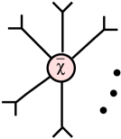
Figure 3: The sum of all purely anti-chiral diagrams vanishes for ${n_{f}}>3$.

We now show that the sum of all purely anti-chiral diagrams, represented in figure 3, vanishes for ${n_{f}}>3$. All but one of the legs of the $\overline{\chi}$ subdiagram has a $D^{2}$ by the Feynamn rules. Rewriting the overall Grassmann integration for $\overline{\chi}$ as $\int d^{4}\theta=\int d^{2}{\overline{\theta}}D^{2}$ gives the remaining leg a $D^{2}$. These $D^{2}$’s combine with the ${\overline{D}}^{2}$’s from each anti-chiral propagator connecting $\overline{\chi}$ to the external vertices to give a factor of $p^{2}$ which cancels the $p^{2}$ in the denominators of those propagators. Thus all the potential IR poles cancel, leaving no $D$’s or ${\overline{D}}$’s to act on the massless external background fields on the external legs.

So, setting the momenta to zero gives a finite result. But, in the $\varepsilon\to 0$ limit, an $SU(2{n_{f}}-2)$ subgroup of the global flavor symmetry is restored. So, the coefficient of the leading power of $\varepsilon$ will be $SU(2{n_{f}}-2)$-invariant. Thus the leading term in the $p^{2}\to 0$ and $\varepsilon\to 0$ limit of the sum of all diagrams of the form shown in figure 3 will be proportional to

$$\epsilon^{u_{1}v_{1}\cdots u_{{n_{f}}-1}v_{{n_{f}}-1}}{\delta{\overline{M}}}_{1u_{1}}{\delta{\overline{M}}}_{2v_{1}}\cdots{\delta{\overline{M}}}_{1u_{{n_{f}}-1}}{\delta{\overline{M}}}_{2v_{{n_{f}}-1}},$$ (38)

since the completely antisymmetric tensor is the only $\mathop{\rm SU}(2{n_{f}}-2)$-invariant way of tying together the flavor indices of the massless external ${\delta{\overline{M}}}$ fields. But the expression in (38) vanishes since the product of the ${\delta{\overline{M}}}_{1u_{i}}$’s and that of the ${\delta{\overline{M}}}_{2v_{i}}$’s are symmetric on their $u_{i}$ and $v_{i}$ indices, respectively.

But this is only the leading term in an expansion around $p^{2}=0$. Higher powers of $p^{2}$ can be brought to act on the external legs, giving derivatives of the external fields in the combinations ${\partial}^{2}({\delta{\overline{M}}}_{1u_{i}}{\delta{\overline{M}}}_{2v_{i}})$. The higher powers of $p^{2}$ come from the Taylor expansion of the $(1+|\varepsilon^{\alpha}|^{2}p^{2})^{-1}$ denominators of the propagators (4.2). Thus each factor of $p^{2}$ comes with a factor of $|\varepsilon|^{2\alpha}$. The flavor symmetry of the leading term in the $\varepsilon$-expansion of the amplitude ensures that the external $u_{i}$ and $v_{i}$ indices are completely antisymmetrized. This still enforces the vanishing of the amplitudes as long as there are at least two factors of $({\delta{\overline{M}}}_{1u_{i}}{\delta{\overline{M}}}_{2v_{i}})$ without derivatives acting on them. Thus, the first non-vanishing term will have a factor of $p^{2}$ acting on ${n_{f}}-2$ pairs of external legs.

Now consider any purely anti-chiral internal sub-diagram $\overline{\chi}$. Each anti-chiral vertex has a $D^{2}$ acting on all but one of its legs as well as an $\int d^{4}\theta_{i}$. Likewise each internal anti-chiral propagator has a ${\overline{D}}^{2}$ as well as a $\delta^{4}(\theta_{i}-\theta_{j})$. The delta functions and Grassmann integrations leave just a single overall $\int d^{4}\theta$. The ${\overline{D}}^{2}$’s and $D^{2}$’s pair up so there is a ${\overline{D}}^{2}D^{2}=p^{2}$ in the numerator of each internal chiral propagator, and a $D^{2}$ acting on all but one of the external legs. This $p^{2}$ cancels the $p^{2}$ in the denominator of the anti-chiral propagator in (4.2), leaving the IR-finite factor proportional to ${\overline{\varepsilon}}^{\alpha}({\overline{\mu}})^{-\beta}({\overline{\lambda}})^{-1}$.

If the purely anti-chiral sub-diagram has $P$ internal propagators, $E$ external legs, and $V_{\ell,0}$ $\ell$-legged vertices, this implies that the whole sub-diagram gives an effective vertex proportional to

$${\overline{\lambda}}^{(-P+\sum_{\ell}V_{\ell,0})}{\overline{\varepsilon}}^{(P\alpha-\sum_{\ell}\gamma_{\ell,0}V_{\ell,0})}{\overline{\mu}}^{(-P\beta-\sum_{\ell}\kappa_{0}V_{\ell,0})}={\overline{\lambda}}{\overline{\varepsilon}}^{-E+(n+1)/n}{\overline{\mu}}^{1/n},$$ (39)

plus terms vanishing as $p^{2}\to 0$. On the right side we have substituted the values of $\alpha$, $\beta$, $\gamma_{\ell,0}$, and $\kappa_{0}$ from (32), (36), and used the identities

$$P+1=\sum_{\ell,m}V_{\ell,m},\qquad 2P+E=\sum_{\ell,m}\ell V_{\ell,m},$$ (40)

where $V_{\ell,m}$ is the number of vertices with a total of $\ell$ legs of which $m$ are massless external legs. They follow from the topology of connected tree diagrams. (We have set the number $m$ of massless external legs to zero because our sub-diagram is internal, so only connects to massive propagators.)

Now we can compute the dependence on $\varepsilon$ of the purely anti-chiral amplitude in figure 3 with $N$ factors of $p^{2}$; it will have an overall factor of $\varepsilon$ to the power of

$$2\alpha N+\left({n+1\over n}-E\right)+({n_{f}}-1)\alpha-({n_{f}}-1)\gamma_{3,2}=(2N-{n_{f}}+1){n-1\over n},$$ (41)

where the first term is from the $N$ factors of $p^{2}$, the second from the $\overline{\chi}$ internal diagram (39) with $E=({n_{f}}-1)$ legs, the third from the $({n_{f}}-1)$ anti-chiral propagators attaching $\overline{\chi}$ to the external 3-vertices and the fourth from the $({n_{f}}-1)$ 3-vertices themselves each with 2 massless legs. We have used the values of $\alpha$ and $\gamma_{3,2}$ from (32) and (36) on the right-hand side. Thus the power of $\varepsilon$ is non-negative when $N\geq({n_{f}}-1)/2$. The minimum value of $N={n_{f}}-2$ needed for the amplitude not to vanish by antisymmetry is greater than $({n_{f}}-1)/2$ for ${n_{f}}>3$. Thus, for ${n_{f}}>3$ the sum of all the diagrams of the form shown in figure 3 vanish as $\varepsilon\to 0$. We evaluated the special ${n_{f}}=3$ case above and saw explicitly that it does not vanish.

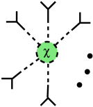
Figure 4: The sum of all diagrams with purely chiral internal vertices.

It remains to evaluate the single diagram in figure 2b. It is a special case of the class of diagrams shown in figure 4: purely-chiral internal diagrams with anti-chiral external 3-vertices. It is easy to evaluate the overall structure of these amplitudes.

The Feynman rules imply that there is a ${\overline{D}}^{2}$ acting on all but one of the ${n_{f}}-1$ legs of the $\chi$ internal sub-diagram. Rewriting the overall Grassmann integration for $\chi$ as $\int d^{4}\theta=\int d^{2}\theta{\overline{D}}^{2}$ gives the remaining leg a ${\overline{D}}^{2}$. Thus each mixed propagator connecting the $\chi$ sub-diagram to the external anti-chiral 3-vertices will have a ${\overline{D}}^{2}$ acting on it. Unlike the purely anti-chiral propagator, the mixed propagator (4.2) has neither an IR pole nor any $D^{2}$’s in the numerator. Thus each ${\overline{D}}^{2}$ will act on a pair of external massless legs. To leading order in the ${\delta{\overline{M}}}$’s, ${\overline{D}}^{2}{\delta{\overline{M}}}=0$ by equation of motion, so we can replace ${\overline{D}}^{2}({\delta{\overline{M}}}^{2})=({\overline{D}}{\delta{\overline{M}}})^{2}$. Thus, the massless external background fields must appear as

$$\int d^{4}xd^{2}\theta\,({\overline{D}}{\delta{\overline{M}}}_{1u_{1}}\cdot{\overline{D}}{\delta{\overline{M}}}_{2v_{1}})\cdots({\overline{D}}{\delta{\overline{M}}}_{1u_{{n_{f}}-1}}\cdot{\overline{D}}{\delta{\overline{M}}}_{2v_{{n_{f}}-1}}).$$ (42)

As before, the leading term in the $\varepsilon\to 0$ limit must be invariant under the $\mathop{\rm SU}(2{n_{f}}-2)$ subgroup of the flavor symmetry that is not broken by the vacuum, and so the $u_{i}$ and $v_{i}$ indices must be contracted with the totally antisymmetric tensor $\epsilon^{u_{1}v_{1}\cdots u_{{n_{f}}-1}v_{{n_{f}}-1}}$.

It is easy to compute the dependence of this amplitude on $\lambda$, $\mu$ and $\varepsilon$. With $E={n_{f}}-1$ external legs, we get from the $\chi$ internal sub-diagram a factor, as in (39),

$$\lambda\varepsilon^{1-{n_{f}}+(n+1)/n}\mu^{1/n};$$ (43)

while the ${n_{f}}-1$ anti-chiral 3-point vertices with 2 massless legs contribute a factor, (35) and (36),

$$({\overline{\lambda}}{\overline{\varepsilon}}^{-2+(n+1)/n}{\overline{\mu}}^{-1+1/n})^{{n_{f}}-1};$$ (44)

and the ${n_{f}}-1$ mixed propagators at $p^{2}=0$ give the factor, (4.2),

$$|\lambda^{-1}\varepsilon^{2-(n+1)/n}\mu^{-1/n}|^{2({n_{f}}-1)}.$$ (45)

Combining all these factors with (42), and recalling that $n={n_{f}}-2$, gives

$$\int d^{4}xd^{2}\theta\,\lambda^{2-{n_{f}}}{\overline{\mu}}^{1-{n_{f}}}\mu^{-1}\epsilon^{u_{1}v_{1}\cdots u_{{n_{f}}-1}v_{{n_{f}}-1}}({\overline{D}}{\delta{\overline{M}}}_{1u_{1}}\cdot{\overline{D}}{\delta{\overline{M}}}_{2v_{1}})\cdots({\overline{D}}{\delta{\overline{M}}}_{1u_{{n_{f}}-1}}\cdot{\overline{D}}{\delta{\overline{M}}}_{2v_{{n_{f}}-1}}),$$ (46)

which is $\varepsilon$-independent. This expression, up to a numerical factor, coincides with (27): the $\mathop{\rm SU}(2)$ superQCD higher-derivative F-terms of [1].

Since this was the only diagram contributing in the ${n_{f}}=4$ case, and since there is only a single diagram in that case, there can be no cancellation of its coefficient. This shows that the ${n_{f}}=4$ singular superpotential indeed reproduces the corresponding higher-derivative global F-term in perturbation theory. With some more work, this argument could be turned into a calculation of the value of the coefficient of the higher-derivative term. But since the normalization of the higher-derivative F-terms was not determined in [1], we are content to have simply shown that the coefficient is non-zero.

4.5 $\bf{n_{f}}\geq 5$

Figure 5: Diagrams for ${n_{f}}=5$ flavors.

As we go higher in the number of flavors, however, the number of diagrams contributing to each amplitude increases. For instance, just among the class of internally purely-chiral diagrams illustrated in figure 4, there are four Feynman diagrams in the case of ${n_{f}}=5$ flavors. As sketched in figure 5, we have one diagram with a single internal vertex, and three different combinations of a diagram with two internal vertices. Although we have shown above that the leading contribution of the sum of these diagrams has the right structure to reproduce the predicted higher-derivative F-term, since now multiple diagrams contribute, we must show in addition that no cancellations occur that could set the coefficient of the higher-derivative term to zero. This seems quite complicated, as it depends on the signs and tensor structures of the vertices. Some sort of symmetry argument is clearly wanted, but still eludes us.

In addition, there are now also other classes of diagrams which are neither purely anti-chiral (as in figure 3) or internally purely chiral (as in figure 4). It is not clear whether these mixed diagrams will also contribute to higher-derivative amplitudes of the form (46) or not.

5 Singular superpotentials in three dimensions

It is worth mentioning that the method we developed here to get the moduli space of the theory from the singular superpotential (5) is not unique to four dimensions. In fact, as we will show below, the method can be used to obtain the moduli space of three dimensional supersymmetric gauge theories (with four supercharges) from singular superpotentials, wherever one is allowed to write such singular superpotenials. See, for example, [19, 20] for discussions of $N=2$ supersymmetric gauge theories in three dimensions.

Consider an $N=2$ $\mathop{\rm SU}(2)$ supersymmetric gauge theory in three dimensions with $2{n_{f}}$ light flavors $Q^{i}_{a}$, transforming in the fundamental representation where $i=1,\cdots,2{n_{f}}$ and $a=1,2$. Classically, the moduli space of the theory has a Coulomb branch as well as a Higgs branch for ${n_{f}}\neq 0$. The Coulomb branch is parameterized by the vacuum expectation values of $U=e^{\Phi}$ where $\Phi$ is a chiral superfield. The scalar component of $\Phi$ is $\phi+i\sigma$, where $\phi\in R/\mathbb{Z}_{2}$ is the scalar in the vector multiplet of the unbroken $\mathop{\rm U}(1)$ and $\sigma\sim\sigma+2\pi r$ is the scalar dual to the gauge field. The Higgs branch is parameterized by the vacuum expectation values of $V^{ij}=\epsilon^{ab}Q^{i}_{a}Q^{j}_{b}$. For ${n_{f}}=1$, $V^{ij}$ is unconstrained while for ${n_{f}}\geq 2$, $V^{ij}$ is subject to rank $(M)\leq 2$, or equivalently

$$\epsilon_{i_{1}\ldots i_{2N_{f}}}V^{i_{1}i_{2}}V^{i_{3}i_{4}}=0,$$ (47)

just as in the four-dimensional case.

The quantum global symmetry of the theory is $\mathop{\rm SU}(2{n_{f}})\times\mathop{\rm U}(1)_{A}\times\mathop{\rm U}(1)_{R}$ under which the fields parametrizing the Coulomb and the Higgs branch transform as

$$\begin{array}[]{c@{\hspace{.1in}\extracolsep{.1in}}ccccl}\hfil\hskip 7.22743pt&\mathop{\rm SU}(2{n_{f}})&{\mathop{\rm U}(1)}_{A}&{\mathop{\rm U}(1)}_{R}&\\[4.30554pt] U\hfil\hskip 7.22743pt&\bf 1&-2{n_{f}}&2(1-{n_{f}})&\\[4.30554pt] V^{ij}\hfil\hskip 7.22743pt&\wedge^{2}({\bf 2{n_{f}}})&2&0&.\\[4.30554pt] \end{array}$$ (48)

For ${n_{f}}\geq 2$, the quantum Higgs branch is the same as the classical Higgs branch, i.e. it is described by (47). We will be interested in the Higgs branch of the moduli space only for ${n_{f}}>2$ where the global symmetry of the theory requires one to consider the singular superpotential [19]

$$W=(1-{n_{f}})(U\ \mbox{Pf}\,V)^{1/({n_{f}}-1)}.$$ (49)

Although this superpotential is singular, it describes the moduli space perfectly for points away from the origin. (There are additional light degrees of freedom at the origin, which are not captured in (49).) To show this, we have to first deform (49), then send the deformation parameters to zero at the end. In close analogy to what we did in four dimensions in section 2, we deform $W$:

$$W\to W^{\zeta,\eta}=W+\zeta U+{1\over 2}\eta_{ij}V^{ij},$$ (50)

where $\zeta$ and $\eta_{ij}$ are some invertible parameters. The equations of motion for $U$ and $V^{kl}$ yield

$$\zeta = \left(U^{2-{n_{f}}}\mbox{Pf}\,V\right)^{1/({n_{f}}-1)},$$

$$V^{kl} = -\left(U\ \mbox{Pf}\,V\right)^{1/({n_{f}}-1)}(\eta^{-1})^{kl}.$$ (51)

Solving the first for $U$ and substituting the result into the second gives an equation for $V^{kl}$ which can be solved to obtain

$$V^{kl}=-\left(\zeta\ \mbox{Pf}\,\eta\right)^{1/2}(\eta^{-1})^{kl}.$$ (52)

Multiplying the above equation by itself and contracting the result with $\epsilon_{i_{1}\ldots i_{2{n_{f}}}}$, we arrive at

$$\epsilon_{i_{1}\ldots i_{2{n_{f}}}}V^{i_{1}i_{2}}V^{i_{3}i_{4}}=\epsilon_{i_{1}\ldots i_{2{n_{f}}}}\zeta\ \mbox{Pf}\,\eta\ (\eta^{-1})^{i_{1}i_{2}}\,(\eta^{-1})^{i_{3}i_{4}}.$$ (53)

The right hand side of (53) is a polynomial of order ${n_{f}}-2>0$ for $\eta_{ij}$ and of order one for $\zeta$. Therefore, independent of how we send $\epsilon_{ij}$ and $\zeta$ to zero, the right hand side of (53) will vanish and we obtain

$$\epsilon_{i_{1}\ldots i_{2{n_{f}}}}V^{i_{1}i_{2}}V^{i_{3}i_{4}}=0,$$ (54)

which is exactly (47), the constraint equation describing the moduli space.

This example gives some evidence that singular superpotentials can also perfectly-well describe the moduli space in supersymmetric gauge theories in three dimensions with four supercharges. A similar argument should also work to describe the moduli space for various $(2,2)$ supersymmetric gauge theories in two dimensions. However, unlike the situation in four dimensions, there is no range of flavors in these lower-dimensional theories where the theory is IR free. This makes a rigorous justification for the existence of the effective superpotentials of these theories harder to come by. In certain cases, like the example discussed above, the lower-dimensional theory can be obtained by compactification of a four-dimensional theory on a circle.

References

- [1] C. Beasley and E. Witten, New instanton effects in supersymmetric QCD, J. High Energy Phys. 0501 (2005) 056, [hep-th/0409149].
- [2] K.A. Intriligator and N. Seiberg, Lectures on supersymmetric gauge theories and electric-magnetic duality, Nucl. Phys. 45BC (Proc. Suppl.) (1996) 1, [hep-th/9509066].
- [3] M.E. Peskin, Duality in supersymmetric Yang-Mills theory, [hep-th/9702094].
- [4] N. Seiberg, Exact results on the space of vacua of four-dimensional SUSY gauge theories, Phys. Rev. D 49 (1994) 6857 [hep-th/9402044].
- [5] K.A. Intriligator and P. Pouliot, Exact superpotentials, quantum vacua and duality in supersymmetric Sp() gauge theories, Phys. Lett. B 353 (1995) 471, [hep-th/9505006].
- [6] N. Seiberg, Electric-magnetic duality in supersymmetric nonabelian gauge theories, Nucl. Phys. B 435 (1995) 129 [hep-th/9411149].
- [7] F. Cachazo, M.R. Douglas, N. Seiberg and E. Witten, Chiral rings and anomalies in supersymmetric gauge theory, J. High Energy Phys. 0212 (2002) 071 [hep-th/0211170].
- [8] N. Seiberg, Adding fundamental matter to ‘Chiral rings and anomalies in supersymmetric gauge theory’, J. High Energy Phys. 0301 (2003) 061, [hep-th/0212225].
- [9] K. Konishi, Anomalous supersymmetry transformation of some composite operators in SQCD, Phys. Lett. B 135 (1984) 439.
- [10] K. Konishi and K.I. Shizuya, Functional integral approach to chiral anomalies in supersymmetric gauge theories, Nuovo Cim. A 90 (1985) 111.
- [11] G. Veneziano and S. Yankielowicz, An effective lagrangian for the pure N=1 supersymmetric Yang-Mills theory, Phys. Lett. B 113 (1982) 231.
- [12] P. C. Argyres and M. Edalati, in preparation.
- [13] E. Witten, An SU(2) anomaly, Phys. Lett. B 117 (1982) 324.
- [14] I. Affleck, M. Dine and N. Seiberg, Dynamical supersymmetry breaking in supersymmetric QCD, Nucl. Phys. B 241 (1984) 493.
- [15] S. Corley, Notes on anomalies, baryons, and Seiberg duality, [hep-th/0305096].
- [16] E. Witten, Chiral ring of Sp(N) and SO(N) supersymmetric gauge theory in four dimensions, [hep-th/0302194].
- [17] P. Svrček, On non-perturbative exactness of Konishi anomaly and the Dijkgraaf-Vafa conjecture, J. High Energy Phys. 0410 (2004) 028, [hep-th/0311238].
- [18] S.J. Gates, M.T. Grisaru, M. Rocek and W. Siegel, Superspace, or one thousand and one lessons in supersymmetry, Benjamin/Cummings 1983, [hep-th/0108200].
- [19] O. Aharony, A. Hanany, K.A. Intriligator, N. Seiberg and M.J. Strassler, Aspects of N = 2 supersymmetric gauge theories in three dimensions, Nucl. Phys. B 499 (1997) 67, [hep-th/9703110].
- [20] J. de Boer, K. Hori and Y. Oz, Dynamics of N = 2 supersymmetric gauge theories in three dimensions, Nucl. Phys. B 500 (1997) 163, [hep-th/9703100].