Graviton emission from a higher-dimensional black hole

Abstract

We discuss the graviton absorption probability (greybody factor) and the cross-section of a higher-dimensional Schwarzschild black hole (BH). We are motivated by the suggestion that a great many BHs may be produced at the LHC and bearing this fact in mind, for simplicity, we shall investigate the intermediate energy regime for a static Schwarzschild BH. That is, for $(2M)^{1/(n-1)}\omega\sim 1$, where $M$ is the mass of the black hole and $\omega$ is the energy of the emitted gravitons in $(2+n)$-dimensions. To find easily tractable solutions we work in the limit $l\gg 1$, where $l$ is the angular momentum quantum number of the graviton.

I Introduction

Much discussion has recently focused on the emission rates of TeV BHs as motivated by the proposition that the quantum gravity scale can be brought down to as low as a TeV in some higher-dimensional BH models GT ; DL ; HHBS . Most cases have focused on the low-energy emission of scalar or spinor fields from higher-dimensional Schwarzschild and slowly rotating Kerr BHs, for a review see reference Krev . Numerical methods also allow us to evaluate the emission in the full energy range Krev .

The importance of bulk emission of gravitons, as well as possible recoil effects, was highlighted recently in references FS1 ; FS2 (also see references Stoj ; FT ). However, little attention has been paid to the actual emission of gravitons from a BH (though there has been some work relating to the quasi-normal modes (QNMs) of higher-dimensional BHs Card1 ; Card2 ; Konop ; Konop2 ; Berti ) and furthermore it is useful to have analytic expressions for the cross-sections etc. not just in the low-energy or high-energy classical regime. In this article we shall discuss BH cross-sections for gravitons in what we shall call the intermediate energy regime for the variable $\varepsilon=2M\omega^{n-1}$, that is where $\varepsilon\sim 1$. In this regime the energy of the particle is near the peak of the potential barrier in the associated scattering problem. The classical cross-section is reproduced in the high-energy limit, $\varepsilon\gg 1$, as we shall discuss later.

In this article we shall focus on the static Schwarzschild BH, though in some models a rotating BH does not necessarily spin-down to zero, but evolves to a non-zero angular momentum Chambers ; NYTM . However, as yet the gravitational perturbation equations for a higher-dimensional rotating BH are unknown. Thus, we shall investigate the intermediate energy regime for the static case, hoping that it may encode some of the properties of the rotating case. Indeed, graviton super-radiance for a large rotation parameter is expected in the intermediate energy regime. To this end only recently has the case of spin-zero emission for the high-energy and high angular momentum regime been studied Harris:2005jx ; Duffy:2005ns , where numerical methods were employed. Note that scalar emission for low-energies and low angular momentum has been studied in references IOP2 ; Frolov .

The particular background we shall investigate is that of a static Schwarzschild BH in $(2+n)$-dimensions. To perform the calculation we shall recall some results recently derived for the gravitational perturbations of a higher-dimensional maximally symmetric BH KI . As mentioned earlier, although it seems likely that TeV BHs will probably be highly rotating when produced NYTM there is not yet a method for separating the gravitational perturbations on a higher-dimensional Kerr background. Thus, we shall content ourselves with the static Schwarzschild case for now.

Gravitational perturbations in general separate into scalar (polar) and vector (axial) perturbations. In more than four-dimensions there is an extra degree of freedom corresponding to tensor perturbations. As shown in reference KI we have for the scalar perturbations;

$$-f\frac{d}{dr}\left(f\frac{d\Phi}{dr}\right)+V_{S}\Phi=\omega^{2}\Phi~{},$$ (1)

where

$$f(r)=1-{2M\over r^{n-1}}$$ (2)

and

$$V_{S}(r)=\frac{f\,H(r)}{16r^{2}[m+\frac{1}{2}n(n+1)(1-f)]^{2}},$$ (3)

with

$$H(r) = \Big{(}n^{4}(n+1)^{2}(1-f)^{3}+n(n+1)\left[4(2n^{2}-3n+4)m+n(n-2)(n-4)(n+1)\right](1-f)^{2}$$ (4)

$$\hskip 28.45274pt-12n\left[(n-4)m+n(n+1)(n-2)\right]m(1-f)+16m^{3}+4n(n+2)m^{2}~{}\Big{)}.$$

In the above

$$m=l_{S}(l_{S}+n-1)-n,\qquad l_{S}=2,3,\,\dots$$ (5)

and as discussed in reference KI the mode $l=0$ corresponds to adding a small mass to the BH; the mode $l=1$ is a pure gauge mode. Note that the true mass of the BH, $M_{\rm BH}$, as measured on the brane, is the same as that in the bulk Tang ; MP and hence;

$$M_{\rm BH}=\frac{n{\cal A}_{n}M}{8\pi c^{2}G_{n+2}}~{},$$ (6)

where

$${\cal A}_{n}={2\pi^{(n+1)/2}\over\Gamma[(n+1)/2]}$$ (7)

is the area of a unit $n$-sphere, $G_{n+2}$ is the $(2+n)$-dimensional Newton constant, and $c$ is the speed of light. In what follows we shall set $G_{n+2}=c=1$.

The vector and tensor perturbations have a much simpler form, which can be written in one concise equation as;

$$-f\frac{d}{dr}\left(f\frac{d\Phi}{dr}\right)+V_{V/T}\Phi=\omega^{2}\Phi~{},$$ (8)

with

$$V_{V/T}(r)=\frac{f}{r^{2}}\left(l(l+n-1)+\frac{n(n-2)}{4}-{\mu_{V/T}\over 4}\frac{n^{2}M}{r^{n-1}}\right)\qquad\qquad\qquad\begin{array}[]{c}l_{V}=2,3,\,\dots\\ l_{T}=1,2,\,\dots\end{array}$$ (9)

where $\mu_{V}=3$ for the vector perturbations, while for the tensor perturbations $\mu_{T}=-1$. Note that the mode $l=1$ of the vector perturbation, which is absent from the above spectrum, represents a purely rotational mode of the BH.

We shall mainly be interested in evaluating the scattering cross-section, which is related to the absorptions probability, $|{\cal A}_{lP}(\omega)|^{2}$, by CCG ;

$$\sigma(\omega)=C{(4\pi)^{(n-1)/2}\over\omega^{n}}\,\Gamma\left({n+1\over 2}\right)\,\sum_{l}^{\infty}\sum_{P}D_{lP}|{\cal A}_{lP}(\omega)|^{2}=\sigma_{S}+\sigma_{V}+\sigma_{T}~{},$$ (10)

where $P$ denotes each respective perturbation and the graviton normalization is CCG ;

$$C={2\over(n+2)(n-1)}~{}.$$ (11)

The degeneracy of each perturbation, $D_{lP}$, is Rubin ;

$$D_{lS}=\frac{(2l+n-1)\,(l+n-2)!}{(n-1)!\,l!}~{},$$

$$D_{lV}=\frac{l(l+n-1)(2l+n-1)(l+n-3)!}{(n-2)!\,(l+1)!}~{},$$

$$D_{lT}=\frac{(n+1)(n-2)(l+n)(l-1)(2l+n-1)(l+n-3)!}{2(n-1)!(l+1)!}~{},$$ (12)

for a given angular momentum channel $l$, which is the spin-2 generalization of the result given in reference Krev . Thus, only scalar and vector perturbations contribute for $n=2$ and the partial sums effectively start from $l=2$, even for the tensor perturbation.

II Intermediate energy approach

To evaluate the absorption probability and hence the graviton emission rate in the intermediate energy regime we shall use the WKB approach of Iyer and Will IW . This was recently used in the higher-dimensional context by Berti et al. Berti (also see reference Card2 ) to investigate the gravitational energy loss of high-energy particle collisions using a QNM analysis. In the following we shall work to lowest order in the generalised WKB method of reference IW ; however, to check the validity of the method we go up to second order to verify that the next order correction is small.

As discussed in reference Berti , in order to use the WKB method we must rewrite the perturbations in the $(n+2)$-dimensional tortoise coordinate defined by;

$$\frac{dr_{*}}{dr}=\frac{1}{f(r)},$$ (13)

which implies that

$$r_{*}=r+\frac{2M}{n-1}\sum_{j=0}^{n-2}\frac{\ln(r/\alpha_{j}-1)}{\alpha_{j}^{n-2}}\,,$$ (14)

where

$$\alpha_{j}=(2M)^{1/(n-1)}{\rm e}^{2\pi{\rm i}j/(n-1)}\qquad(j=0,\dots,n-2)\,.$$ (15)

The tortoise coordinate, $r_{*}$, given above becomes quite complicated in more than four-dimensions and in our case it will be more convenient to work with the original coordinate $r$ and use equation (13) to convert derivatives. Thus the perturbation equations reduce to the standard Schrödinger form;

$$\left(\frac{d^{2}}{dr_{*}^{2}}+Q_{P}(r_{*})\right)\Phi=0\,,\qquad\qquad Q_{P}(r_{*})=\omega^{2}-V_{P}(r_{*}).$$ (16)

The subscript $P$ denotes any one of the three possible perturbations. Note that the potential, equation (3), is defined in terms of $r$ and not $r_{*}$, the tortoise coordinate.

As discussed in reference IW , an adapted form of the WKB method can be employed to find the QNMs or the absorption probability, which we are primarily interested in, when the scattering takes place near the top of the potential barrier. In the following we shall use the same notation as reference IW . The absorption probability, up to second order in the WKB expansion, is found to be;

$$|{\cal A}_{l}(\omega)|^{2}={1\over 1+e^{2i\pi(\nu+1/2)}}~{},$$ (17)

where

$$\nu+1/2=i(2Q_{P_{0}}^{\prime\prime})^{-1/2}Q_{P_{0}}-\Lambda$$ (18)

and

$$\Lambda=i(2Q_{P_{0}}^{\prime\prime})^{-1/2}\left(\left[\frac{3}{8}\left({Q^{(4)}_{P_{0}}\over 12Q_{P_{0}}^{\prime\prime}}\right)-\frac{7}{32}\left({Q^{{}^{\prime\prime\prime}}_{P_{0}}\over 3Q_{P_{0}}^{\prime\prime}}\right)^{2}\right]+(\nu+1/2)^{2}\left[\frac{6}{4}\left({Q^{(4)}_{P_{0}}\over 12Q_{P_{0}}^{\prime\prime}}\right)-\frac{30}{16}\left({Q^{{}^{\prime\prime\prime}}_{P_{0}}\over 3Q_{P_{0}}^{\prime\prime}}\right)^{2}\right]\right)\,,$$ (19)

these being parameters determined in reference IW , and where the subscript zero denotes the maximum of $-\,Q(r_{*})$.

By substituting equation (19) into equation (18) we can eliminate $\Lambda$ to obtain an expression solely in terms of $\nu+1/2$; however, because we wish to only know the size of the second order correction we can eliminate $\nu+1/2$ to find $\Lambda$;

$$\Lambda=\frac{1}{2C}\left(1+2AC\pm\sqrt{1+4(A-B)C}~{}\right)\,,$$ (20)

where

$$A=i(2Q_{P_{0}}^{\prime\prime})^{-1/2}Q_{P_{0}},$$ (21)

and

$$B=i(2Q_{P_{0}}^{\prime\prime})^{-1/2}\left[\frac{3}{8}\left({Q^{(4)}_{P_{0}}\over 12Q_{P_{0}}^{\prime\prime}}\right)-\frac{7}{32}\left({Q^{{}^{\prime\prime\prime}}_{P_{0}}\over 3Q_{P_{0}}^{\prime\prime}}\right)^{2}\right],\qquad\qquad C=i(2Q_{P_{0}}^{\prime\prime})^{-1/2}\left[\frac{6}{4}\left({Q^{(4)}_{P_{0}}\over 12Q_{P_{0}}^{\prime\prime}}\right)-\frac{30}{16}\left({Q^{{}^{\prime\prime\prime}}_{P_{0}}\over 3Q_{P_{0}}^{\prime\prime}}\right)^{2}\right]~{}.$$ (22)

In general it is just a simple but tedious exercise in algebra to evaluate the second order correction. However, as we discuss in the next section, by considering the potential to leading order, ${\cal O}(l^{0})$, we can estimate the size of the second order correction without making any explicit calculations.

III Zeroth-order approximation

To illustrate the method as simply as possible let us work to zeroth order in the WKB expansion for the case of large $l$. However, in order to find a difference between the respective perturbations we should consider up to $O(l^{0})$ in the potential, which in this case is given by;

$$V_{S}(r)\approx{f\over r^{2}}\left(l^{2}+(n-1)l+\frac{n(n-2)}{4}+{n\over 4}(8-7n)(1-f)\right)\,,$$ (23)

for the scalar perturbation and

$$V_{V/T}(r)=\frac{f}{r^{2}}\left(l^{2}+(n-1)l+\frac{n(n-2)}{4}-\frac{\mu}{4}n^{2}(1-f)\right)\,,$$ (24)

for the vector and tensor potential, which is an exact expression to ${\cal O}(l^{0})$, see equation (9). Importantly, we can immediately notice that in four-dimensions, $n=2$, the scalar and vector potentials are identical to ${\cal O}(l^{0})$. The equivalence of the scalar and vector potentials for general $l$ is well known in four-dimensions Chandra , however, as discussed in reference KI , this is not true for the case of general dimensions. This will have important consequences for the graviton emission of a higher-dimensional BH, which we shall discuss later. For convenience let us write a general formula for all the perturbations, valid up to $O(l^{0})$;

$$V_{P}(r)=\frac{f(r)}{r^{2}}\left(\hat{l}^{2}+\beta-\frac{\alpha_{P}}{4}(1-f)\right),\qquad\mathrm{where}\qquad\hat{l}^{2}=l^{2}+(n-1)l\qquad\qquad\forall~{}l=2,3,\,\dots~{}.$$ (25)

In the previous equation we have used;

$$\beta={n(n-2)\over 4},$$ (26)

and

$$\alpha_{S}=n(7n-8),\qquad\qquad\alpha_{V}=3n^{2},\qquad\qquad\alpha_{T}=-n^{2}~{}.$$ (27)

At this stage it will be convenient to change variables to $z=\omega r$, for example see reference PS , and by doing so the WKB equation now becomes;

$$\left(\frac{d^{2}}{dz_{*}^{2}}+Q_{P}(z_{*})\right)\Phi=0\,,\qquad\qquad Q_{P}(z_{*})=1-V_{P}(z_{*})\,,$$ (28)

where

$$V_{P}(z)=\frac{f(z)}{z^{2}}\left(\hat{l}^{2}+\beta-\frac{\alpha_{P}}{4}{\varepsilon\over z^{n-1}}\right),$$ (29)

and

$$f(z)=1-{\varepsilon\over z^{n-1}}\,;\qquad\qquad\varepsilon=2M\omega^{n-1}\,.$$ (30)

The expression for the absorption probability, equation (17), is defined explicitly in terms of derivatives of the potential with respect to the tortoise coordinate $z_{*}$ (or $r_{*}$, where $z_{*}$ has been defined in an analogous way to $r_{*}$); however, in terms of $z$, up to second order in derivatives of the potential, we find;

$${dQ\over dz_{*}} = {dz\over dz_{*}}{dQ\over dz}=f(z){dQ\over dz}=\left(1-{\varepsilon\over z^{n-1}}\right){dQ\over dz}~{},$$ (31)

$${d^{2}Q\over dz^{2}_{*}} = f(z){d\over dz}\left(f(z){dQ\over dz}\right)=\left(1-{\epsilon\over z^{n-1}}\right)\,\left(z^{-n}\left(-1+n\right)\,\epsilon\,{dQ\over dz}+\left(1-{\epsilon\over z^{n-1}}\right)\,{d^{2}Q\over dz^{2}}\right)~{}.$$ (32)

Note that at the maximum of the potential, $z_{0}$, the first term in equation (32) is zero and thus simplifies our calculation.

Hence, from equation (18) with $\Lambda=0$, we are easily lead to the result;

$$|{\cal A}_{lP}|^{2}={1\over 1+e^{{2\pi\over K}\big{[}f(z_{0})\left(\hat{l}^{2}+\beta-\frac{\alpha}{4}\,\varepsilon{{z_{0}}}^{1-n}\right)-z_{0}^{2}\big{]}}}\,,$$ (33)

where we have written the general perturbation as;

$$K(\hat{l},z_{0},\varepsilon) = {(z_{0}^{n}-\varepsilon\,z_{0})\over{\sqrt{2}}\,{{z_{0}}}^{2\,n}}{\sqrt{-2\,n\,\left(1+2\,n\right)\,\alpha\,{\epsilon}^{2}\,{{z_{0}}}^{2}-24\,\left(\hat{l}^{2}+\beta\right)\,{{z_{0}}}^{2\,n}+\left(2+3\,n+n^{2}\right)\,\left(4\,\hat{l}^{2}+\alpha+4\,\beta\right)\,\epsilon\,{{z_{0}}}^{1+n}}}\,$$

and we have dropped the subscript $P$ for clarity. Choosing the appropriate $\alpha_{P}$ from equation (27) then determines the absorption probability for each respective perturbation mode. The location of the maximum, $z_{0}$, for the potential $-\,Q_{P}(z_{0})$ can also be solved, see appendix A. This also depends on the type of perturbation.

Before we proceed any further we should verify that the second order correction is small as compared to the zeroth order one. Given that $V_{P}$ is of order ${\cal O}(l^{2})$, see equation (25), and that $l$ is independent of $r$ or $r_{*}$, it is simple to see that;

$$i(2Q_{P_{0}}^{\prime\prime})^{-1/2}\sim{\cal O}(l^{-1})~{}.$$ (35)

The terms in the square brackets for $B$ and $C$, see equation (22), are of ${\cal O}(l^{0})$ and hence (using the relation above) $B$ and $C$ contribute to order ${\cal O}(l^{-1})$. Furthermore the term $A$ is of order ${\cal O}(l)$. Thus the second order contribution, $\Lambda$, see equation (20), is of order ${\cal O}(l^{-1})$ and is therefore negligible in the limit $l\gg 1$. This is also true for the high-energy limit $\varepsilon\gg 1$, as well as for intermediate energies $\varepsilon\sim 1$.

IV Results

In this section we shall present our results as based on the analytic expressions derived in the previous section. Furthermore we shall also demonstrate that the geometric optics limit is reproduced for large values of $\varepsilon$. Note that for completeness we shall also derive this expression.

We have presented our first set of results in Fig. 1 where we have plotted the absorption probability as a function of $l$ for each of the perturbations. We have also considered scenarios involving different dimensions, $n$, for $\varepsilon\sim 1$. Firstly, the scalar mode has the largest contribution, followed by the vector and then the tensor perturbations; however, this does depend on the value of $\varepsilon$. Secondly, we see that the absorption probability is larger for smaller $n$. In fact numerical plots for different $\varepsilon$ show that $|{\cal A}_{lP}|^{2}$ saturates to unity for larger and larger $l$ as $\varepsilon$ increases. This implies that larger $l$ is required in the angular momentum sum for the cross-section, when obtaining the geometric optics limit, see below.

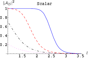
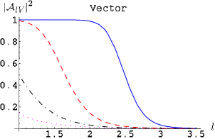
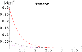
Figure 1: Black hole absorption probability, $|{\cal A}_{lP}|^{2}$, as a function of angular momentum $l$ (extended to real numbers) for $\varepsilon=1$. Blue (solid), red (dashed), black (dot-dashed) and purple (dotted) curves correspond to $n=2,3,4$ and $5$ respectively. Note that the scalar and vector perturbations are only valid from $l=2$ onwards, however, for comparison with the tensor case we start at $l=1$.

Turning to the cross-section, as given by;

$$\sigma(\omega)=C\,(4\pi)^{(n-1)/2}\,\Gamma\left({n+1\over 2}\right)\,\left({2M\over\varepsilon}\right)^{n\over n-1}\sum_{l=2}^{\infty}\sum_{P}{D_{lP}\over 1+e^{{2\pi\over K}\big{[}f(z_{0})\left(\hat{l}^{2}+\beta-\frac{\alpha}{4}\,\varepsilon{{z_{0}}}^{1-n}\right)-z_{0}^{2}\big{]}}}~{},$$ (36)

where $D_{lP}$ is given in equation (I) and remembering that $\alpha=\alpha_{P}$. It should be noted that though we are primarily interested in the intermediate energy regime, $\varepsilon\sim 1$, with large angular momentum, $l\gg 1$, the above expression can also be applied to the case where $l>\varepsilon^{1/(n-1)}\sim 1$. Note also that although the next order correction in the WKB expansion becomes larger for $l\sim{\cal O}(1)$ we can still extrapolate the results hoping the errors are not too large. In Fig. 2 we plot the cross-section, equation (36), as a function of $\varepsilon$ and to ensure convergence in the partial wave sums we sum up to $l_{max}\sim 3\,\varepsilon_{max}$. The total cross-section tends to the classical one for large $\varepsilon$ as we shall now explain.

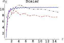
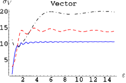
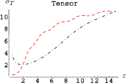
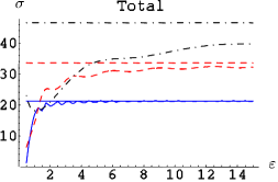
Figure 2: Black hole cross-sections as a function of $\varepsilon$, in units of $(2M)^{n\over n-1}$, for each gravitational perturbation and the total one. The horizontal lines correspond to the classical cross-section. Blue (solid), red (dashed) and black (dot-dashed) curves correspond to $n=2,3$ and $4$ respectively. Note that there is no tensor perturbation for the $n=2$ case.

In the intermediate energy approach (for large $l$) the absorption probabilities satisfy $A_{lS}=A_{lV}=A_{lT}$, see Fig. 1, and the degeneracies satisfy CCG ;

$$D_{lS}\approx C\left(D_{lS}+D_{lV}+D_{lT}\right)~{}.$$ (37)

Furthermore, the classical cross-section corresponds to the high-energy limit, $\varepsilon^{1/(n-1)}\gg l\gg 1$, which then implies the absorption coefficients $A_{lP}\sim{\cal O}(1)$ and in this limit the sum over $l$ has a cut-off at $l\approx b\,\omega$ (for example, see reference DeWitt ) where $b$ is the critical radius (or impact parameter) at which the BH ceases to absorb radiation. This is given by equation (12) of reference EHM , for a massless/relativistic particle as;

$$b=\left(n+1\over 2\right)^{1\over n-1}\left(n+1\over n-1\right)^{1\over 2}(2M)^{1\over n-1}~{}.$$ (38)

Given the cut-off in the mode sum we have;

$$\sum_{l}^{b\omega}D_{lS}\sim{2(b\omega)^{n}\over n!}$$ (39)

for large $\omega$, and substituting this into equation (36), using (37), leads to the classical cross-section;

$$\sigma_{c}={(4\pi)^{(n-1)/2}\over\omega^{n}}\,\Gamma\left({n+1\over 2}\right){2(b\omega)^{n}\over n!}={2\sqrt{\pi}(\pi)^{n-1\over 2}\over n\Gamma(n/2)}\left(n+1\over 2\right)^{n\over n-1}\left(n+1\over n-1\right)^{n\over 2}(2M)^{n\over n-1}~{},$$ (40)

where in the second step we used the gamma duplication formula. This agrees with the standard result in $(2+n)$-dimensions, compare with reference Krev (after making the substitution $r_{H}^{n-1}=2M$).

As is well known, the high-energy cross-section is independent of the particle species, and likewise we see that it is independent of the graviton cross-section. These are represented by horizontal lines in the bottom right plot in Fig. 2 and we see that our analytic results correctly reproduce the high-energy limit $\varepsilon\gg 1$ (note that for higher-dimensions larger values of $\varepsilon$ are required to obtain the geometric optics limit).

V Conclusion

In conclusion we have shown in this paper that the WKB method of Iyer and Will IW can be applied to the case of graviton emission from a Schwarzschild BH. Indeed our results reproduce the classical cross-section in the high-energy limit. We have also presented new results for the intermediate energy regime.

In the low-energy limit, $M\omega\ll 1$, our method breaks down as can be seen from Fig. 2, where the cross-section starts to diverge. It is well known that the cross-section is proportional to $\omega^{2l+n}$ in $(2+n)$-dimensions Krev , which essentially corresponds to $s$-wave scattering for a spin-zero field, as the lowest $l$ modes dominate the cross-section. Indeed it is straightforward to obtain the low-energy cross-section for the vector and tensor perturbations by employing the standard technique of matching the near horizon and far field solutions, for example using the techniques discussed in references KR ; Unruh ; alstar . However, there is a subtlety with the higher-dimensional Zerilli (scalar) equation: In four-dimensions the Regge-Wheeler (vector) solution is usually used to find the absorption probability, which is equivalent to that for the Zerilli equation, as the two solutions are identical in four-dimensions Chandra , but as pointed out in reference KI , in higher dimensions no such relation exists. Thus, if we attempt to use the standard technique of matching the near horizon and far field solutions directly for the Zerilli equation it appears that numerical methods seem more amenable. Regardless, the focus of this current work has been the intermediate energy regime given that this is where we expect graviton emission to be most interesting for a rapidly rotating BH.

Although in this article we focused on the static Schwarzschild BH, we can also apply our method to the case of spin-zero field emission from a Kerr BH CJNS2 . Note that though the solution to the graviton perturbations for a higher-dimensional Kerr BH have not yet been found, we are encouraged by the fact that there are some similarities between the total graviton and spin-0 cross-sections, see Appendix B. As can be seen from Fig. 3, the total cross-section, which is the sum of the perturbations (scalar, vector and tensor) is of the same order of magnitude as the spin-0 case, i.e. $O(\sigma_{S}+\sigma_{V}+\sigma_{T})\sim O(\sigma_{B})$, and such an approximation may also be valid for the rotating case.

The rotating case is particularly interesting due to the phenomenon of super-radiance (for example see reference alstar ), where the absorption probability becomes negative. Super-radiance has been discussed in the higher-dimensional context recently in references Harris:2005jx ; NYTM ; IOP2 ; Duffy:2005ns ; Frolov . However, the highly rotating case has only been considered using numerical techniques; whereas we expect that our approach allows for an analytic expression for such a case. Furthermore, our approach should also allow one to evaluate the QNMs analytically for the rapidly rotating case, as has recently been done in the limit $a\to\infty$ CSY . In the four-dimensional case the rotation parameter $a=1$ is bounded to $a_{\rm max}=1$, for example see reference Chandra . This fact has meant that there have been no prior investigations of the QNMs of a Kerr BH with a large rotation parameter. However, in $(2+n)$-dimensions there are $(n+1)/2$ rotation parameters, where for $n>3$ the rotation parameters are unbounded MP . Indeed, as we mentioned, even after the spin-down phase in some models the BH remains rotating Chambers ; NYTM .

Another interesting case for which the WKB method can be applied is that for emission from a charged (Reisner-Nordstrom) BH. Recently the graviton perturbations have been found in reference KI2 (along with their QNMs Konop2 ). However, in this case the solutions are complicated by the fact that there are now solutions for the electromagnetic field itself. We hope to present results for this model in the near future.

Appendix A Location of the maximum, $Q_{P_{0}}$

In order to find the maximum of the potential it is convenient to work with the coordinate;

$$x=1-f={2M\over r^{n-1}}\,,$$ (41)

rather than $r_{*}$ or $r$. That is we wish to find the roots of;

$$0={dV_{P}\over dr_{*}}={dr\over dr_{*}}{dV_{P}\over dr}=(1-n)(2M)^{1\over 1-n}(1-x)x^{n\over n-1}~{}{dV_{P}\over dx}.$$ (42)

Here we should mention that in our case, even though all the expressions depend on $Q_{P}$, the potential can be written in the form $Q_{P}=\omega^{2}-V_{P}$ and thus, for a given energy, $\omega$, the maximum of $-Q_{P}$ corresponds to the maximum of $V_{P}$.

Therefore, apart from the solutions at the horizon ($x=1$) and at infinity ($x=0$), we merely require the roots of;

$${dV_{P}\over dx}=0~{}.$$ (43)

Working to $O(l)$ in the potential allows the maximum to be easily found;

$$x_{0}^{P}={2\over n+1}\,,$$ (44)

which is a result valid for all three perturbations. However, as we have previously discussed, in order to see a difference between the perturbations we must work to order $O(l^{0})$. Hence, for the gravitational perturbations we obtain;

$$x_{0}^{P}=\frac{\left(1+n\right)\,\left(4\,\hat{l}^{2}+\alpha+4\,\beta\right)-{\sqrt{-64\,n\,\alpha\,\left(\hat{l}^{2}+\beta\right)+{\left(1+n\right)}^{2}\,{\left(4\,\hat{l}^{2}+\alpha+4\,\beta\right)}^{2}}}}{4\,n\,\alpha}\,,$$ (45)

where, as before, we are using the shorthand notation $\hat{l}^{2}=l^{2}+(n-1)l$ and the coefficients $\alpha$ and $\beta$ (ignoring the subscripts) as defined in equation (27). Note that if we expand the square root in powers of large $l$ we obtain equation (44).

The location of the maximum in terms of the coordinates $r$ and $z$ is then simply given by;

$$r_{0}^{P}=\left(2M\over x_{0}^{P}\right)^{1\over n-1}\qquad\mathrm{and}\qquad z_{0}^{P}=\omega r_{0}^{P}=\left(\varepsilon\over x_{0}^{P}\right)^{1\over n-1}\,,$$ (46)

which is independent of the perturbation up to $O(l)$, see equation (44).

Appendix B Spin-Zero Emission

In this appendix we briefly discuss the case of emission of a bulk scalar (spin-zero) field. As we shall see the effective potential is equivalent to that for the tensor perturbations. Following reference KR , after a separation of variables, the scalar radial equation, $g^{\mu\nu}\nabla_{\mu}\nabla_{\nu}\,\phi(x)=0$, is found to be;

$$\frac{f(r)}{r^{n}}\,\frac{d\,}{dr}\,\biggl{[}\,f(r)\,r^{n}\,\frac{dR(r)}{dr}\,\biggr{]}+\biggl{[}\,\omega^{2}-\frac{f(r)}{r^{2}}\,l\,(l+n-1)\,\biggr{]}R(r)=0\,.$$ (47)

This equation can be written in the WKB form by applying the tortoise coordinate defined in equation (13) and rescaling the radial solution by $R(r_{*})=r^{-n/2}\Phi(r_{*})$. A short calculation leads to;

$$\frac{d^{2}\,\Phi^{2}}{dr_{*}^{2}}+\omega^{2}\,\Phi(r_{*})-\frac{f(r)}{r^{2}}\left[l(l+n-1)+{n\over 4}(n-2)+{n^{2}\over 4}(1-f)\right]\Phi(r_{*})=0,\qquad\qquad l_{B}=0,1,2,\dots$$ (48)

One can then easily verify that this equation is identical to that for the tensor perturbations of the graviton, see equation (9); however, the degeneracy factor, $D_{lP}$, will be different. The only difference between the two being that the sum over $l$ starts from $l=0$ for a spin-zero field, not $l=2$.

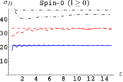
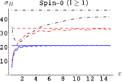
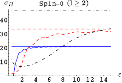
Figure 3: Black hole cross-section for the graviton compared to a spin-zero field as a function of $\varepsilon$, in units of $(2M)^{n\over n-1}$. The horizontal lines correspond to the classical cross-section. Blue (solid), red (dashed) and black (dot-dashed) curves correspond to $n=2,3$ and $4$ respectively.

In Fig. 3 we compare the spin-zero cross-section, $\sigma_{B}$, with the total graviton cross-section. Although the classical cross-sections agree in the high-energy limit (asymptotically), at intermediate energies they do not agree due to differences in the partial wave sums. However, at lower energies we see that by taking the spin-0 cross-section from $l=1$ we obtain the best agreement with that for the graviton, see Fig. 3. Note that for further comparison we also plot the spin-0 cross-section with the partial sum starting from $l=2$.

References

- (1) S. B. Giddings and S. Thomas, Phys. Rev. D 65 (2002) 056010 [arXiv:hep-ph/0106219].
- (2) S. Dimopoulos and G. Landsberg, Phys. Rev. Lett. 87 (2001) 161602 [arXiv:hep-ph/0106295].
- (3) S. Hossenfelder, S. Hofmann, M. Bleicher and H. Stoecker, Phys. Rev. D 66 (2002) 101502 [arXiv:hep-ph/0109085].
- (4) P. Kanti, Int. J. Mod. Phys. A 19 (2004) 4899 [arXiv:hep-ph/0402168].
- (5) V. P. Frolov and D. Stojkovic, Phys. Rev. D 66 (2002) 084002 [arXiv:hep-th/0206046].
- (6) V. P. Frolov and D. Stojkovic, Phys. Rev. Lett. 89 (2002) 151302 [arXiv:hep-th/0208102].
- (7) D. Stojkovic, Phys. Rev. Lett. 94 (2005) 011603 [arXiv:hep-ph/0409124].
- (8) A. Flachi and T. Tanaka, Phys. Rev. Lett. 95 (2005) 161302 [arXiv:hep-th/0506145].
- (9) V. Cardoso, O. J. C. Dias and J. P. S. Lemos, Phys. Rev. D 67 (2003) 064026 [arXiv:hep-th/0212168].
- (10) R. A. Konoplya, Phys. Rev. D 68 (2003) 024018 [arXiv:gr-qc/0303052].
- (11) R. A. Konoplya, Phys. Rev. D 68 (2003) 124017 [arXiv:hep-th/0309030].
- (12) V. Cardoso, J. P. S. Lemos and S. Yoshida, Phys. Rev. D 69 (2004) 044004 [arXiv:gr-qc/0309112].
- (13) E. Berti, M. Cavaglia and L. Gualtieri, Phys. Rev. D 69 (2004) 124011 [arXiv:hep-th/0309203].
- (14) C. M. Chambers, W. A. Hiscock and B. Taylor, Phys. Rev. Lett. 78 (1997) 3249 [arXiv:gr-qc/9703018].
- (15) H. Nomura, S. Yoshida, M. Tanabe and K. i. Maeda, Prog. Theor. Phys. 114 (2005) 707 [arXiv:hep-th/0502179].
- (16) C. M. Harris and P. Kanti, arXiv:hep-th/0503010.
- (17) G. Duffy, C. Harris, P. Kanti and E. Winstanley, JHEP 0509 (2005) 049 [arXiv:hep-th/0507274].
- (18) V. P. Frolov and D. Stojkovic, Phys. Rev. D 67 (2003) 084004 [arXiv:gr-qc/0211055].
- (19) D. Ida, K. y. Oda and S. C. Park, Phys. Rev. D 67 (2003) 064025 [Erratum-ibid. D 69 (2004) 049901] [arXiv:hep-th/0212108]; ibid. D 71 (2005) 124039 [arXiv:hep-th/0503052].
- (20) H. Kodama and A. Ishibashi, Prog. Theor. Phys. 110 (2003) 701 [arXiv:hep-th/0305147].
- (21) F. Zerilli, Phys. Rev. Lett. 24 (1970) 737; Phys. Rev. D 2 (1970) 2141.
- (22) T. Regge, and J. Wheeler, Phys. Rev. 108 (1957) 1063.
- (23) F. R. Tangherlini, Nuovo Cimento 27, 636 (1963).
- (24) R. C. Myers and M. J. Perry, Annals Phys. 172 (1986) 304.
- (25) V. Cardoso, M. Cavaglia and L. Gualtieri, arXiv:hep-th/0512002; ibid. arXiv:hep-th/0512116.
- (26) A. Chodos and E. Myers, Annals Phys. 156 (1984) 412; M. A. Rubin and C. R. Ordonez, J. Math. Phys. 25 (1984) 2888; ibid. J. Math. Phys. 26 (1985) 65; I. G. Moss, “Quantum theory, black holes and inflation,” Wiley Press.
- (27) S. Iyer and C. M. Will, Phys. Rev. D 35 (1987) 3621.
- (28) S. Chandrasekhar, “The Mathematical Theory Of Black Holes,” Clarendon Press, Oxford (1985).
- (29) E. Poisson and M. Sasaki, Phys. Rev. D 51 (1995) 5753 [arXiv:gr-qc/9412027].
- (30) B. S. DeWitt, Phys. Rept. 19 (1975) 295.
- (31) R. Emparan, G. T. Horowitz and R. C. Myers, Phys. Rev. Lett. 85 (2000) 499 [arXiv:hep-th/0003118].
- (32) P. Kanti and J. March-Russell, Phys. Rev. D 66 (2002) 024023 [arXiv:hep-ph/0203223].
- (33) W. G. Unruh, Phys. Rev. D 14 (1976) 3251.
- (34) A. A. Starobinsky, JETP 37, 28 (1973); A. A. Starobinsky and S.M. Churilov, JETP 38, 1 (1973).
- (35) A. S. Cornell, J. Doukas, W. Naylor and M. Sasaki, in progress.
- (36) V. Cardoso, G. Siopsis and S. Yoshida, Phys. Rev. D 71 (2005) 024019 [arXiv:hep-th/0412138].
- (37) H. Kodama and A. Ishibashi, Prog. Theor. Phys. 111 (2004) 29 [arXiv:hep-th/0308128].