Supersymmetric Deformations of Type IIB Matrix Model as Matrix Regularization of ${\cal N}=4$ SYM

Abstract:

We construct a ${\cal Q}=1$ supersymmetry and $U(1)^{5}$ global symmetry preserving deformation of the type IIB matrix model. This model, without orbifold projection, serves as a nonperturbative regularization for ${\cal N}=4$ supersymmetric Yang-Mills theory in four Euclidean dimensions. Upon deformation, the eigenvalues of the bosonic matrices are forced to reside on the surface of a hypertorus. We explicitly show the relation between the noncommutative moduli space of the deformed matrix theory and the Brillouin zone of the emergent lattice theory. This observation makes the transmutation of the moduli space into the base space of target field theory clearer. The lattice theory is slightly nonlocal, however the nonlocality is suppressed by the lattice spacing. In the classical continuum limit, we recover the ${\cal N}=4$ SYM theory. We also discuss the result in terms of D-branes and interpret it as collective excitations of D(-1) branes forming D3 branes.

1 Introduction

The study of supersymmetric deformations of the type IIB matrix model (or IKKT matrix model [1]) is interesting both from the field theory and string theory points of view. The deformations may alter the classical moduli spaces into noncommutative spaces, and hence, may form a bridge between zero dimensional, finite rank matrix theories and higher dimensional regularized quantum field theories. In this work, we show such a correspondence between a ${\cal Q}=1$ supersymmetry and $U(1)^{5}$ global symmetry preserving deformation of type IIB matrix model, and ${\cal N}=4$ supersymmetric Yang-Mills theory in four dimensions. Mainly, the deformed type IIB matrix model serves as finite $N_{c}$ matrix regularization (which will be shown to be equivalent to a lattice regularization), where $N_{c}$ is the number of colors, for ${\cal N}=4$ supersymmetric Yang-Mills theory in four dimensions. This construction can be thought as supersymmetric generalization of the relation between twisted Eguchi-Kawai (TEK) and four dimensional lattice gauge theory [2, 3].

The essential point of the construction is the relation between two seemingly different concepts. The noncommutative moduli space of vacua, which is the zero action configuration of the deformed bosonic action, and the noncommutative base space, the space that the target field theory lives in. In the type IIB theory without deformation, the eigenvalues of the bosonic matrices can be anywhere in the moduli space. The deformations, that will be considered in this paper, alter the structure of moduli space in such a way that the eigenvalues of bosonic matrices are forced to reside on the surface of a four dimensional hypertorus, $T^{4}$. This is essential for the emergence of four dimensional spacetime and will be discussed in detail in sections 3 and 4.1.

In the description of the deformed type IIB action in section 2, we use the notation introduced in [4], which makes the $SU(5)\times U(1)$ subgroup of global $SO(10)$ R-symmetry and ${\cal Q}=1$ supersymmetry manifest. Therefore, we use five complex matrices $z^{m}$ and their hermitian conjugates $\kern 0.6pt\overline{\kern-0.6ptz\kern-0.6pt}\kern 0.6pt_{m}$ as the bosonic degrees of freedom instead of ten bosonic hermitian matrices. This notation is more akin to our four dimensional habits and the bosonic action becomes just a sum of D-term and F-terms, which are derivatives of superpotential. The bosonic action of the deformed type IIB matrix model is given by

$$S_{bosonic} =\frac{\operatorname{Tr\,}}{g^{2}}\bigg{[}\frac{1}{2}\bigg{(}\sum_{m=1}^{5}[\kern 0.6pt\overline{\kern-0.6ptz\kern-0.6pt}\kern 0.6pt_{m},z^{m}]\bigg{)}^{2}+\sum_{m\neq n=1}^{5}|e^{-i\Phi_{mn}/2}\kern 0.6pt\overline{\kern-0.6ptz\kern-0.6pt}\kern 0.6pt_{m}\kern 0.6pt\overline{\kern-0.6ptz\kern-0.6pt}\kern 0.6pt_{n}-e^{i\Phi_{mn}/2}\;\kern 0.6pt\overline{\kern-0.6ptz\kern-0.6pt}\kern 0.6pt_{n}\kern 0.6pt\overline{\kern-0.6ptz\kern-0.6pt}\kern 0.6pt_{m}|^{2}\bigg{]}$$ (1)

where the antisymmetric phase matrix $\Phi_{mn}$ are the deformation parameters. This change in the action may be considered as the deformation of the “superpotential”. The action Eq. (1) may be obtained by the dimensional reduction of the four dimensional hypercubic lattice action of ${\cal N}=4$ SYM to zero volume (a point) upon the use of twisted boundary conditions. The phases $\Phi_{\mu\nu}$, where $\mu,\nu=1,\ldots,4$, are associated with electric and magnetic background fluxes [5] and $\Phi_{\mu 5}=-\sum_{\alpha=1}^{4}\Phi_{\mu\alpha}$. We will show that a two parameter family of deformation which, for example, corresponds to electric and magnetic fields in z-direction, suffices to generate the target ${\cal N}=4$ theory .

The technique described here is different from the recent constructions of lattice regularization for extended supersymmetric Yang-Mills theories [11, 12, 13, 4] and deconstruction of six dimensional theories [14, 15]. The current approach does not require orbifold projection of a mother theory. As it will be shown explicitly, the deformation of the mother theory becomes the lattice regularization. Recall that the orbifold projected matrices are sparse and encode a commutative spacetime lattice. In our approach the spacetime lattice is generated by the zero action configurations of the deformed type IIB matrix model and there are no constraints on our matrix variables. Similarly, based on [11] and [16, 3], the lattice action for noncommutative counterparts of the extended supersymmetric gauge theories are also constructed, by using orbifolds with discrete torsion, in [17] for spatial and [18] for Euclidean two dimensional lattices. (For recent progress and independent approaches on supersymmetric gauge theories on lattice, also see [19, 20]. For a review on discrete torsion, see [21] and the references in [18])

To show the equivalence of the deformed type IIB matrix model to the four dimensional theory on a discrete torus, we decompose the bosonic matrices into a background and fluctuations around it. By using the background field techniques, it is possible to exhibit that the fluctuations around the zero action configurations can be identified as a lattice action on a four dimensional discrete torus. This action has many parallels to the lattice action in ref.[4]. The main difference with respect to the action in [4] is the noncommutativity of the base space lattice, which can be traded with the nonlocalness of the interactions. However, we show that two types of finite-volume continuum limits are possible. In a particular scaling of the deformation parameter (in which the noncommutativity length tends to zero with respect to the linear extent of the box), the interaction localizes in the position space and the outcome is ordinary local field theory. In the limit where the noncommutativity length is nonvanishing, the outcome is nonlocal ${\cal N}=4$ SYM.

It is also possible to interpret the result of this paper within string theory. The main result can be understood as a collective excitation of a finite number of D(-1)-branes to generate discretized D3-brane(s) wrapped on a four dimensional hypertorus. Notice that we do not use compactification (see [22] for a review) to generate the higher dimensional theory. Also, our D(-1)-brane configurations are inherently different from the BPS-saturated backgrounds discussed in [23] , which have typically finite action and are unstable at finite $N_{c}$. We discuss this direction briefly in section 5. The rest of the paper is organized as follows: In section 2 and appendix A, we set the notation and derive the deformed type IIB action. In section 3, we analyze the noncommutative moduli space and make the relation with TEK more explicit. In section 4, we show that the the deformed type IIB action can be rewritten as a lattice action and obtain the classical continuum limit.

2 The type IIB matrix model and its supersymmetric deformations

The type IIB matrix model can be obtained by the dimensional reduction of the ten dimensional ${\cal N}=1$ $U(N_{c})$ supersymmetric Yang-Mills theory to zero dimension. The theory possess a $G_{R}=SO(10)$ global R-symmetry, inherited by the (Euclidean) Lorentz symmetry of the ten dimensional theory. The bosonic and fermionic degrees of freedom of the matrix theory are in vector (${\bf 10}$) and positive chirality spinor (${\bf 16}$) representations of $SO(10)$. The action of the type IIB matrix model is conventionally expressed as

$$S=-\frac{1}{g^{2}}\sum_{\alpha\neq\beta=1}^{10}\frac{1}{4}\operatorname{Tr\,}\ [v_{\alpha},v_{\beta}]^{2}+\frac{i}{2}\operatorname{Tr\,}\omega^{T}C\Gamma_{\alpha}[v_{\alpha},\omega]$$ (2)

where $v_{\alpha}=v_{\alpha}^{a}t^{a}$ is a Hermitian matrix and $\omega=\omega^{a}t^{a}$ is a 32-component spinor which has only its upper sixteen component nonvanishing. The ten gamma matrices $\Gamma_{\alpha}$ form a chiral basis of $SO(10)$ and $C$ is charge conjugation matrix. The Lie algebra generators are normalized such that $\operatorname{Tr\,}t^{a}t^{b}=\delta^{ab}$. This action respects ${\cal Q}=16$ supersymmetries generated by $\delta v_{\alpha}=-\kappa^{T}C\Gamma_{\alpha}\omega,\;\;{\rm and}\;\;\delta\omega=\frac{i}{4}[v_{\alpha},v_{\beta}]\;[\Gamma_{\alpha},\Gamma_{\beta}]\kappa$ , where $\kappa$ is a positive chirality Grassmann spinor.

We aim to construct deformations of the type IIB matrix model, which preserves ${\cal Q}=1$ supersymmetry and $U(1)^{5}$ global symmetry. Since the bosonic variables that appear in the action Eq. (2) are not eigenstates of the $U(1)^{5}$, this form of the action is not adequate for our purpose. The type IIB action, in terms of eigenstates of $SU(5)\times U(1)$, which provides the right basis for our purpose, is constructed in [4] and is outlined in the next section.

The motivation behind this construction is to obtain a finite rank matrix regularization of ${\cal N}=4$ SYM theory in four dimensions. It is well-known that the TEK model is a matrix regularization of (noncommutative) Yang-Mills theories in even dimensions. Our goal here is to construct a fully supersymmetric counterpart of this relation. It is, therefore, important to construct the supersymmetric matrix model analog of TEK. The TEK is obtained by dimensional reduction of a fully regulated lattice gauge theory to a single site by using the twisted boundary conditions. We will follow the same strategy and reduce the lattice regulated ${\cal N}=4$ SYM to a single point.

2.1 ${\cal N}=4$ SYM on hypercubic lattice

In order to construct the deformed Type IIB matrix model, we start with the four dimensional hypercubic orbifold lattice. In [4], the lattice action of ${\cal N}=4$ SYM is given for both $A_{4}^{*}$ lattice and hypercubic lattice. Here, we will use hypercubic for convenience. The dimensional reduction of the lattice to a single site by using periodic boundary conditions reproduces the type IIB matrix model in the eigenbasis of $U(1)^{5}$ symmetry. The reduction by using twisted boundary conditions gives the deformed Type IIB action.

$p$-cell fields orientations 0-cell $\lambda$ $0$ 1-cell $z^{\mu},\psi^{\mu};\qquad\kern 0.6pt\overline{\kern-0.6ptz\kern-0.6pt}\kern 0.6pt_{\mu}$ ${\bf\hat{e}_{\mu}};\qquad{-\bf\hat{e}_{\mu}}$ 2-cell $\xi_{\mu\nu}$ ${-\bf\hat{e}_{\mu}-\hat{e}_{\nu}}$ 3-cell $\xi^{\nu\rho\sigma}$ ${\bf\hat{e}_{\nu}+\hat{e}_{\rho}+\hat{e}_{\sigma}}={-\bf\hat{e}_{\mu}-\hat{e}_{5}}$ 4-cell $(z_{\mu\nu\rho\sigma},\psi_{\mu\nu\rho\sigma});\qquad\kern 0.6pt\overline{\kern-0.6ptz\kern-0.6pt}\kern 0.6pt^{\mu\nu\rho\sigma}$ ${\bf\hat{e}}_{5}=-\sum_{\mu=1}^{4}{\bf\hat{e}}_{\mu};\qquad-{\bf\hat{e}}_{5}$

Table 1: The distribution of the bosonic and fermionic fields to the $p$-cells of the hypercubic lattice. Each field is totally antisymmetric in its indices. For convenience, we will also use $\xi^{\nu\rho\sigma}={\epsilon^{\nu\rho\sigma\mu}}\xi_{\mu 5}$, $(z_{\mu\nu\rho\sigma},\psi_{\mu\nu\rho\sigma})=\epsilon_{\mu\nu\rho\sigma}(z^{5},\psi^{5})$, and $\kern 0.6pt\overline{\kern-0.6ptz\kern-0.6pt}\kern 0.6pt^{\mu\nu\rho\sigma}=\epsilon^{\mu\nu\rho\sigma}\kern 0.6pt\overline{\kern-0.6ptz\kern-0.6pt}\kern 0.6pt_{5}$. The cartesian basis vectors are given by $({\bf\hat{e}}_{\mu})_{\nu}=\delta_{\mu\nu}$ where $\mu,\nu=1,\ldots 4$ .

Let us first rewrite the action of the ${\cal N}=4$ SYM theory in $d=4$ dimensional hypercubic lattice and establish our notation. The fundamental cell of a hypercubic lattice contains one site, four links, six faces, four cubes and one hypercube, collectively called $p$-cells. There are bosonic and fermionic fields associated with each $p$-cell. For a $d=4$ dimensional lattice, the total number of $p$-cells in a unit-cell is

$$2^{4}=\sum_{r=0}^{4}\binom{4}{k}=1\oplus 4\oplus 6\oplus 4\oplus 1$$ (3)

The fermions, which form the ${\bf 16}$ dimensional spinor representation of the $SO(10)$ are distributed among the $p$-cells. The labeling of the fermions follows the name of cell that it lives in: $\omega\sim{\bf 16}=\lambda\oplus\psi^{\mu}\oplus\xi_{\mu\nu}\oplus\xi^{\mu\nu\rho}\oplus\psi_{\mu\nu\rho\sigma}=1\oplus 4\oplus 6\oplus 4\oplus 1$ where each fermion is totally antisymmetric tensor and they reside on sites, links, diagonal of faces, diagonal of the cubes, and the body diagonal of the hypercube [24] The upper and lower indices determine the orientation of the fermionic link field (see Table.1). For notational convenience and brevity, we introduce $\xi_{\mu 5}=\frac{\epsilon_{\mu\nu\rho\sigma}}{3!}\xi^{\nu\rho\sigma}$ and $\psi^{5}=\frac{\epsilon_{\mu\nu\rho\sigma}}{4!}\psi^{\mu\nu\rho\sigma}$.

The bosons, which form a ${\bf 10}$ dimensional vector representation of $SO(10)$ are associated with 1-cells and body diagonal of 4-cells. We have $v_{\alpha}\sim{\bf 10}=z^{\mu}\oplus\kern 0.6pt\overline{\kern-0.6ptz\kern-0.6pt}\kern 0.6pt_{\mu}\oplus z_{\mu\nu\rho\sigma}\oplus\kern 0.6pt\overline{\kern-0.6ptz\kern-0.6pt}\kern 0.6pt^{\mu\nu\rho\sigma}=4\oplus\kern 0.6pt\overline{\kern-0.6pt4\kern-0.6pt}\kern 0.6pt\oplus 1\oplus 1$. For convenience, we rename $z^{5}=\frac{\epsilon^{\mu\nu\rho\sigma}}{4!}z_{\mu\nu\rho\sigma}$ and $\kern 0.6pt\overline{\kern-0.6ptz\kern-0.6pt}\kern 0.6pt_{5}=\frac{\epsilon_{\mu\nu\rho\sigma}}{4!}\kern 0.6pt\overline{\kern-0.6ptz\kern-0.6pt}\kern 0.6pt^{\mu\nu\rho\sigma}$ .

Naturally, the ${\cal Q}=1$ superfields on the hypercubic lattice are associated with $p$-cells. The component form of the superfields and the $p$-cell that they are residing in are given as

$$0-{\rm cell}:\qquad{\bf\Lambda}_{{\bf n}}=\lambda_{{\bf n}}-i\theta d_{{\bf n}}\ ,$$ (4)

$$1-{\rm cells}:\qquad{\mathbf{Z}}^{\mu}_{{\bf n}}=z^{\mu}_{{\bf n}}+\sqrt{2}\,\theta\,\psi^{\mu}_{{\bf n}}\ ,\qquad\kern 0.6pt\overline{\kern-0.6ptz\kern-0.6pt}\kern 0.6pt_{\mu,{\bf n}}$$

$$2-{\rm cells}:\qquad{\bf\Xi}_{\mu\nu,{\bf n}}=\xi_{\mu\nu,{\bf n}}-2\theta\,\,\kern 0.6pt\overline{\kern-0.6ptE\kern-0.6pt}\kern 0.6pt_{{\mu\nu},{\bf n}}$$

$$3-{\rm cells}:\qquad{\bf\Xi}_{\mu 5,{\bf n}}=\xi_{\mu 5,{\bf n}}-2\theta\,\,\kern 0.6pt\overline{\kern-0.6ptE\kern-0.6pt}\kern 0.6pt_{{\mu 5},{\bf n}}$$

$$4-{\rm cell}:\qquad{\mathbf{Z}}^{5}_{{\bf n}}=z^{5}_{{\bf n}}+\sqrt{2}\,\theta\,\psi^{5}_{{\bf n}}\ ,\qquad\kern 0.6pt\overline{\kern-0.6ptz\kern-0.6pt}\kern 0.6pt_{5,{\bf n}}$$

where the $\kern 0.6pt\overline{\kern-0.6ptz\kern-0.6pt}\kern 0.6pt_{\mu,{\bf n}}$ and $\kern 0.6pt\overline{\kern-0.6ptz\kern-0.6pt}\kern 0.6pt_{5,{\bf n}}$ are supersymmetry singlets and the $d_{\bf n}$ is an auxiliary field. The antiholomorphic functions $\kern 0.6pt\overline{\kern-0.6ptE\kern-0.6pt}\kern 0.6pt_{{\mu\nu},{\bf n}}$ and $\kern 0.6pt\overline{\kern-0.6ptE\kern-0.6pt}\kern 0.6pt_{{\mu\nu},{\bf n}}$ are given by

$$\kern 0.6pt\overline{\kern-0.6ptE\kern-0.6pt}\kern 0.6pt_{{\mu\nu},{\bf n}}=\kern 0.6pt\overline{\kern-0.6ptz\kern-0.6pt}\kern 0.6pt_{\mu,{\bf n}+{\bf\hat{e}_{\nu}}}\kern 0.6pt\overline{\kern-0.6ptz\kern-0.6pt}\kern 0.6pt_{\nu,{\bf n}}-\kern 0.6pt\overline{\kern-0.6ptz\kern-0.6pt}\kern 0.6pt_{\nu,{\bf n}+{\bf\hat{e}_{\mu}}}\kern 0.6pt\overline{\kern-0.6ptz\kern-0.6pt}\kern 0.6pt_{\mu,{\bf n}}$$ (5)

$$\kern 0.6pt\overline{\kern-0.6ptE\kern-0.6pt}\kern 0.6pt_{{\mu 5},{\bf n}}=\kern 0.6pt\overline{\kern-0.6ptz\kern-0.6pt}\kern 0.6pt_{\mu,{\bf n}+{\bf\hat{e}_{5}}}\kern 0.6pt\overline{\kern-0.6ptz\kern-0.6pt}\kern 0.6pt_{5,{\bf n}}-\kern 0.6pt\overline{\kern-0.6ptz\kern-0.6pt}\kern 0.6pt_{5,{\bf n}+{\bf\hat{e}_{\mu}}}\kern 0.6pt\overline{\kern-0.6ptz\kern-0.6pt}\kern 0.6pt_{\mu,{\bf n}}$$ (6)

The antiholomorphic $\kern 0.6pt\overline{\kern-0.6ptE\kern-0.6pt}\kern 0.6pt$ functions are supersymmetry singlets as well since they only depend on $\kern 0.6pt\overline{\kern-0.6ptz\kern-0.6pt}\kern 0.6pt$, but not $z$. They can be thought as zero dimensional counterpart of the superpotential (more precisely, the F-term)

The hypercubic lattice action may be written in manifestly ${\cal Q}=1$ supersymmetric form as in [4]

$$S = \frac{\operatorname{Tr\,}}{g^{2}}\sum_{\bf n}\bigg{[}\int\;d\theta\left(-\frac{1}{2}{\bf\Lambda_{\bf n}}{\partial}_{\theta}{\bf\Lambda_{\bf n}}-{\bf\Lambda_{\bf n}}(\kern 0.6pt\overline{\kern-0.6ptz\kern-0.6pt}\kern 0.6pt_{m,\bf{n-\hat{e}_{m}}}{\bf Z}_{m,\bf{n-\hat{e}_{m}}}-{\bf Z}_{m,\bf n}\kern 0.6pt\overline{\kern-0.6ptz\kern-0.6pt}\kern 0.6pt_{m,\bf n})+\frac{1}{2}{\bf\Xi}_{mn,\bf n}{\bf E}_{mn,\bf n}\right)$$ (7)

. $$+ \bigg{.}\frac{\sqrt{2}}{8}\epsilon^{mnpqr}{\bf\Xi}_{mn,\bf n}(\kern 0.6pt\overline{\kern-0.6ptz\kern-0.6pt}\kern 0.6pt_{p,\bf{n-\hat{e}_{p}}}{\bf\Xi}_{qr,\bf{n+\hat{e}_{m}+\hat{e}_{n}}}-{\bf\Xi}_{qr,\bf{n-\hat{e}_{q}-\hat{e}_{r}}}\kern 0.6pt\overline{\kern-0.6ptz\kern-0.6pt}\kern 0.6pt_{p,\bf{n+\hat{e}_{m}+\hat{e}_{n}}})\bigg{]}\qquad\qquad$$ (8)

where the holomorphic ${\bf E}$ functions are

$${\bf E}_{mn,{\bf n}}=({\bf Z}_{m,\bf n}{\bf Z}_{n,\bf{n+\hat{e}_{m}}}-{\bf Z}_{n,\bf n}{\bf Z}_{m,\bf{n+\hat{e}_{n}}})\;.$$ (9)

The ${\bf E}$ function is a function of superfields $\mathbf{Z}$ and has a $\theta$ expansion where the lowest component of ${\bf E}$ is the minus hermitian conjugate of $\kern 0.6pt\overline{\kern-0.6ptE\kern-0.6pt}\kern 0.6pt$:

$${\bf E}=E+\theta\partial_{m}E\psi^{m},\qquad\kern 0.6pt\overline{\kern-0.6ptE\kern-0.6pt}\kern 0.6pt=-{E}^{\dagger}$$ (10)

Notice that the last term in the action is not integrated over the superspace, yet it is respectful to ${\cal Q}=1$ supersymmetry. It is not hard to show that the $\theta$ component of the last term is identically zero due to Jacobi identity, and translational invariance of the lattice action. Hence it is supersymmetric.

The dimensional reduction of the lattice action Eq. (8) to a single site by imposing the periodic boundary conditions (for example $\Lambda_{\bf{n+\hat{e}_{\mu}}}=\Lambda_{\bf{n}}$) and by integrating out the auxiliary $d$ field yields the type IIB matrix theory action Eq. (2) expressed in terms of $SU(5)\times U(1)$ multiplets

$$S =\frac{\operatorname{Tr\,}}{g^{2}}\bigg{[}(\frac{1}{2}\sum_{m=1}^{5}\ [\kern 0.6pt\overline{\kern-0.6ptz\kern-0.6pt}\kern 0.6pt_{m},z_{m}])^{2}+\sum_{m,n=1}^{5}|[z_{m},z_{n}]|^{2}$$ (11)

. $$\bigg{.}+\lambda[\kern 0.6pt\overline{\kern-0.6ptz\kern-0.6pt}\kern 0.6pt_{m},\psi^{m}]-\frac{1}{2}{\xi}_{mn}[z^{m},\psi^{n}])+\frac{\sqrt{2}}{8}\epsilon^{mnpqr}\xi_{mn}[\kern 0.6pt\overline{\kern-0.6ptz\kern-0.6pt}\kern 0.6pt_{p},\xi_{qr}]\bigg{]}\,.$$ (12)

This action is merely a rewriting of Eq. (2), in terms of a new set of variables. Recall that Eq. (2) is expressed in terms of $SO(10)$ multiplets, vector ${\bf 10}$ and positive chirality spinor ${\bf 16}$. We could have obtained Eq. (12) from Eq. (2) by just employing the decompositions $v_{\alpha}\sim{\bf 10}\rightarrow z^{m}\oplus\bar{z}_{m}\sim{\bf 5}\oplus{\bf\kern 0.6pt\overline{\kern-0.6pt5\kern-0.6pt}\kern 0.6pt}$ for bosons, and $\omega\sim{\bf 16}\rightarrow\lambda\oplus\psi^{m}\oplus\xi_{mn}\sim{\bf 1}\oplus{\bf 5}\oplus{\bf\kern 0.6pt\overline{\kern-0.6pt10\kern-0.6pt}\kern 0.6pt}$ for fermions into $SU(5)$ multiplets as in ref.[4]. The dimensional reduction is used to set the notation and for later convenience.

Notice that the bosonic matrix model takes a form similar to the potential in $d=4$ dimensional ${\cal N}=1$ supersymmetric theories. There the potential is a sum of $d$ and $F$ (derivative of the superpotential) term contributions in the $\frac{d^{2}}{2}+|F|^{2}$ form. In the zero dimensional matrix model expressed in manifest ${\cal Q}=1$ superfields, the role of $F$ is replaced with the $E$ functions and the bosonic action can be written as

$$S_{bosonic}=\frac{d^{2}}{2}+id\,[{\kern 0.6pt\overline{\kern-0.6ptz\kern-0.6pt}\kern 0.6pt}_{m},z^{m}]+\sum_{m\neq n=1}^{5}|\kern 0.6pt\overline{\kern-0.6ptE\kern-0.6pt}\kern 0.6pt_{mn}|^{2}$$ (13)

where $E^{mn}=[\,z^{m},z^{n}\,]$. The deformation that we will construct in the next section will alter $E$, but not the $d$ term.

2.2 Dimensional reduction and twisted boundary conditions

To formulate the deformed type IIB model, we start with the lattice action Eq. (8) of the ${\cal N}=4$ SYM theory in four dimensional hypercube. Then we reduce the lattice theory to a single site by imposing the twisted boundary conditions. This is indeed the same philosophy used in the construction of the twisted Eguchi-Kawai model [2].

The difference between deformed Type IIB and TEK is that in ${\cal N}=4$ lattice action, there is a superfield associated with each $p$-cell. Hence, there are many gauge invariant plaquettes terms possible, which are shown in fig.2 and fig.1, and will be explained momentarily. In TEK, we only have unitary link (1-cell) fields and the only possible gauge invariant plaquette terms are the square plaquette terms.

In reducing the lattice action Eq. (8) to a single point by using twisted boundary conditions, we request periodicity modulo gauge rotations $g_{\mu}$. Let $\Psi$ be a a generic field associated with a $p$-cell on the lattice. We utilize

$$\Psi_{\bf{n+\hat{e}_{\nu}}}=g_{\nu}\Psi_{\bf{n}}g_{\nu}^{\dagger}\,,$$ (14)

$$\Psi_{\bf{n+\hat{e}_{\mu}+\hat{e}_{\nu}}}=g_{\mu}g_{\nu}\Psi_{\bf{n}}g_{\nu}^{\dagger}g_{\mu}^{\dagger}\,,$$ (15)

$$\Psi_{\bf{n+\hat{e}_{\mu}+\hat{e}_{\nu}+\hat{e}_{\rho}}}=g_{\mu}g_{\nu}g_{\rho}\Psi_{\bf{n}}g_{\rho}^{\dagger}g_{\nu}^{\dagger}g_{\mu}^{\dagger}\,,$$ (16)

$$\Psi_{\bf{n+\hat{e}_{5}}}=g_{5}\Psi_{\bf{n}}g_{5}^{\dagger},\qquad{\rm where}\qquad g_{5}=(\prod_{\nu=1}^{4}g_{\nu})^{\dagger},$$ (17)

and then set $\Psi_{\bf{n}}$ to a site independent value. The global gauge rotation matrices $g_{\mu}$ satisfy the ’t Hooft algebra [5]

$$g_{\mu}g_{\nu}=e^{i\Phi_{\mu\nu}}g_{\nu}g_{\mu},\qquad{\rm equivalently},\qquad e^{-i\Phi_{\mu\nu}/2}g_{\mu}g_{\nu}=e^{i\Phi_{\mu\nu}/2}g_{\nu}g_{\mu}\,.$$ (18)

The antisymmetric $\Phi_{\mu\nu}$ matrix is identified as the flux passing through the $\mu\nu$ plane. More precisely, $\Phi_{\mu\nu}\equiv 2\pi\frac{n_{\mu\nu}}{N_{c}}$ where $n_{\mu\nu}$ is an integer associated with the integer electric ($n_{4i}$) or magnetic ($n_{ij}$) flux modulo $N_{\rm c}$. Also, note that $\Psi_{\bf{n-\hat{e}_{\nu}}}=g_{\nu}^{\dagger}\Psi_{\bf{n}}g_{\nu}$. The second form of the equation Eq. (18) is symmetric under the exchange $\mu\leftrightarrow\nu$ and will be more useful in appendix. The commutation relation of $g_{\mu}$ with $g_{5}$ is given by

$$g_{\mu}g_{5}=e^{i\Phi_{\mu 5}}g_{5}g_{\mu},\qquad{\rm where}\qquad\Phi_{\mu 5}=-\sum_{\alpha\neq\mu}^{4}\Phi_{\mu\alpha}$$ (19)

The $\Phi_{\mu 5}$ is the flux passing through the plaquette whose boundary is an oriented parallelogram (generalization of the one shown in fig.2 to four dimensions), whose sides are the link piercing the 4-cell, and the link along the 1-cell. Such a plaquette has a nonvanishing projection on three faces, and has zero projected area on the other three face which are orthogonal to the $\mu$ direction. Hence, the flux passing through it, is the sum of fluxes passing through the faces, which this plaquette has non-vanishing projection, i.e, $\Phi_{\mu 5}=-\sum_{\alpha\neq\mu}^{4}\Phi_{\mu\alpha}$. The two commutation relations, Eq. (18) and Eq. (19), can be combined into $g_{m}g_{n}=e^{i\Phi_{mn}}g_{n}g_{m}$ by keeping in mind the definition of $g_{5}$ and $\Phi_{mn}$.

The reduction of the orbifold lattice action Eq. (8) to a single site by using twisted boundary condition gives the action of the deformed Type IIB matrix model. The derivation of this action is given in the appendix A. However, the deformed action is easy to understand on physical grounds. Here we present a heuristic argument.

First, note that the lattice action Eq. (8) is a sum of a $Q$-exact and a $Q$-closed expression. Schematically, both types are triangular plaquette terms whose sides are bosonic (B) and fermionic (F) ${\cal Q}=1$ supermultiplets. Upon reduction and appropriate field redefinitions, all the commutators will be replaced by “deformed commutators”, where the deformation parameter is the flux passing through the corresponding triangular plaquettes:

$$S_{exact}\sim{F[\;B_{1},B_{2}\;]}|_{\theta}\rightarrow F[e^{i({\rm flux})}B_{1}B_{2}-e^{-i({\rm flux})}B_{1}B_{2}]|_{\theta}$$ (20)

$$S_{closed}\sim{F_{1}[\;B,F_{2}\;]}\rightarrow F_{1}[e^{i({\rm flux})}BF_{2}-e^{-i({\rm flux})}F_{2}B]$$ (21)

Since there are $p$-form supermultiplets which reside on the diagonal of each $p$-cell, there are a number of possible plaquettes. The fluxes associated with each type of plaquette will be different. We first write down the deformed type IIB action in manifestly ${\cal Q}=1$ superfields and by preserving the $U(1)^{5}$ global symmetry, and then we explain the plaquette structures. The deformed action, which is the main result of this paper, is given by

$$S_{deformed}=\frac{1}{g^{2}}\operatorname{Tr\,}\int d\theta\bigg{(}-\frac{1}{2}{\bf\Lambda}{\partial}_{\theta}{\bf\Lambda}-{\bf\Lambda}([\kern 0.6pt\overline{\kern-0.6ptz\kern-0.6pt}\kern 0.6pt_{\mu},{\bf Z}^{\mu}]+\frac{1}{24}\;[\kern 0.6pt\overline{\kern-0.6ptz\kern-0.6pt}\kern 0.6pt^{\mu\nu\rho\sigma},{\bf Z}_{\mu\nu\rho\sigma}])\bigg{.}$$ (22)

$$\bigg{.}+\frac{1}{2}{\bf\Xi}_{\mu\nu}(e^{-i\Phi_{\mu\nu}/2}{\bf Z}^{\mu}{\bf Z}^{\nu}-e^{i\Phi_{\mu\nu}/2}{\bf Z}^{\nu}{\bf Z}^{\mu})\bigg{.}$$ (23)

$$\bigg{.}+\frac{1}{12}{\bf\Xi}^{\nu\rho\sigma}(e^{i(\Phi_{\mu\nu}+\Phi_{\mu\rho}+\Phi_{\mu\sigma})/2}{\bf Z}^{\mu}{\bf Z}_{\mu\nu\rho\sigma}-e^{-i(\Phi_{\mu\nu}+\Phi_{\mu\rho}+\Phi_{\mu\sigma})/2}{\bf Z}_{\mu\nu\rho\sigma}{\bf Z}^{\mu})\bigg{)}$$ (24)

$$+\frac{\sqrt{2}}{2}{\bf\Xi}_{\mu\nu}(e^{i(\Phi_{\rho\mu}+\Phi_{\rho\nu})/2}\;\kern 0.6pt\overline{\kern-0.6ptz\kern-0.6pt}\kern 0.6pt_{\rho}\;{\bf\Xi}^{\mu\nu\rho}-e^{-i(\Phi_{\rho\mu}+\Phi_{\rho\nu})/2}\;{\bf\Xi}^{\mu\nu\rho}\kern 0.6pt\overline{\kern-0.6ptz\kern-0.6pt}\kern 0.6pt_{\rho})$$ (25)

$$+\frac{\sqrt{2}}{8}{\bf\Xi}_{\mu\nu}(e^{-i(\Phi_{\rho\mu}+\Phi_{\rho\nu}+\Phi_{\sigma\mu}+\Phi_{\sigma\nu})/2}\;\kern 0.6pt\overline{\kern-0.6ptz\kern-0.6pt}\kern 0.6pt^{\mu\nu\rho\sigma}\,\,{\bf\Xi}_{\rho\sigma}-e^{i(\Phi_{\rho\mu}+\Phi_{\rho\nu}+\Phi_{\sigma\mu}+\Phi_{\sigma\nu})/2}\;{\bf\Xi}_{\rho\sigma}\kern 0.6pt\overline{\kern-0.6ptz\kern-0.6pt}\kern 0.6pt^{\mu\nu\rho\sigma})\qquad$$ (26)

In this expression, the penultimate and the last line are not separately supersymmetric, but their sum add up to a $Q$-closed form and supersymmetric. The ${\cal Q}=1$ off-shell supersymmetry transformations can then be realized in terms of the following superfields, each of which is the reduction of the $p$-form field to a single point

$${\bf\Lambda} = \lambda-\theta id,$$ (27)

$${\bf Z}^{\mu} = z^{\mu}+\sqrt{2}\theta\psi^{\mu},\qquad\kern 0.6pt\overline{\kern-0.6ptz\kern-0.6pt}\kern 0.6pt_{\mu},$$ (28)

$${\bf\Xi}_{\mu\nu} = \xi_{\mu\nu}-2\theta{\kern 0.6pt\overline{\kern-0.6ptE\kern-0.6pt}\kern 0.6pt}_{\mu\nu}(\kern 0.6pt\overline{\kern-0.6ptz\kern-0.6pt}\kern 0.6pt),$$ (29)

$${\bf\Xi}_{\mu 5} = \xi_{\mu 5}-2\theta{\kern 0.6pt\overline{\kern-0.6ptE\kern-0.6pt}\kern 0.6pt}_{\mu 5}(\kern 0.6pt\overline{\kern-0.6ptz\kern-0.6pt}\kern 0.6pt)\;\;({\bf\Xi}^{\nu\rho\sigma}),$$ (30)

$${\bf Z}^{5} = z^{5}+\sqrt{2}\theta\psi^{5}\;\;({\bf Z}_{\mu\nu\rho\sigma}),\qquad\kern 0.6pt\overline{\kern-0.6ptz\kern-0.6pt}\kern 0.6pt_{5}\;\;({\kern 0.6pt\overline{\kern-0.6ptz\kern-0.6pt}\kern 0.6pt}^{\mu\nu\rho\sigma}),$$ (31)

where $\kern 0.6pt\overline{\kern-0.6ptz\kern-0.6pt}\kern 0.6pt_{m}$ are supersymmetry singlets. The $\kern 0.6pt\overline{\kern-0.6ptE\kern-0.6pt}\kern 0.6pt$ functions are given by

$${\kern 0.6pt\overline{\kern-0.6ptE\kern-0.6pt}\kern 0.6pt}_{\mu\nu}(\kern 0.6pt\overline{\kern-0.6ptz\kern-0.6pt}\kern 0.6pt) =e^{-i\Phi_{\mu\nu}/2}\;\kern 0.6pt\overline{\kern-0.6ptz\kern-0.6pt}\kern 0.6pt_{\mu}\kern 0.6pt\overline{\kern-0.6ptz\kern-0.6pt}\kern 0.6pt_{\nu}-e^{+i\Phi_{\mu\nu}/2}\;\kern 0.6pt\overline{\kern-0.6ptz\kern-0.6pt}\kern 0.6pt_{\nu}\kern 0.6pt\overline{\kern-0.6ptz\kern-0.6pt}\kern 0.6pt_{\mu}$$ (32)

$${\kern 0.6pt\overline{\kern-0.6ptE\kern-0.6pt}\kern 0.6pt}_{\mu 5}(\kern 0.6pt\overline{\kern-0.6ptz\kern-0.6pt}\kern 0.6pt) =e^{i\sum_{\nu\neq\mu}\Phi_{\mu\nu}/2}\;\kern 0.6pt\overline{\kern-0.6ptz\kern-0.6pt}\kern 0.6pt_{\mu}\kern 0.6pt\overline{\kern-0.6ptz\kern-0.6pt}\kern 0.6pt_{5}-e^{-i\sum_{\nu\neq\mu}\Phi_{\mu\nu}/2}\;\kern 0.6pt\overline{\kern-0.6ptz\kern-0.6pt}\kern 0.6pt_{5}\kern 0.6pt\overline{\kern-0.6ptz\kern-0.6pt}\kern 0.6pt_{\mu}$$ (34)

and they give rise to deformed potential of the matrix theory. The $\kern 0.6pt\overline{\kern-0.6ptE\kern-0.6pt}\kern 0.6pt$ functions are supersymmetry singlets since they are functions of $\kern 0.6pt\overline{\kern-0.6ptz\kern-0.6pt}\kern 0.6pt$ and not $\mathbf{Z}$, and are annihilated by the only supersymmetry in the theory: $Q\kern 0.6pt\overline{\kern-0.6ptE\kern-0.6pt}\kern 0.6pt=0$. Similarly, the functions ${\bf E}$ are functions of general ${\cal Q}=1$ superfields, and are given by

$${\bf E}^{\mu\nu}=e^{-i\Phi_{\mu\nu}/2}\;\mathbf{Z}^{\mu}\mathbf{Z}^{\nu}-e^{i\Phi_{\mu\nu}/2}\;\mathbf{Z}^{\nu}\mathbf{Z}^{\mu}$$ (35)

$${\bf E}^{\mu 5}=e^{-i\Phi_{\mu 5}/2}\;\mathbf{Z}^{\mu}\mathbf{Z}^{5}-e^{i\Phi_{\mu 5}/2}\;\mathbf{Z}^{5}\mathbf{Z}^{\mu}$$ (36)

Notice that, as before, ${\bf E}$ has an expansion in superspace and the lowest component of ${\bf E}$ is negative hermitian conjugate of $\kern 0.6pt\overline{\kern-0.6ptE\kern-0.6pt}\kern 0.6pt$, i.e; $\kern 0.6pt\overline{\kern-0.6ptE\kern-0.6pt}\kern 0.6pt=-{E}^{\dagger}$.

The rest of this paper is devoted to the study of the deformed action Eq. (26). Even though it is not apparent at first glance, it serves as a matrix regularization of the four dimensional ${\cal N}=4$ SYM theory. This identification requires neither orbifold projection nor compactification [22]. We will show how Eq. (26) gives rise to the four dimensional ${\cal N}=4$ SYM theory, both commutative and non-commutative. In order to do that, it is important to understand the structure of the noncommutative moduli space, i.e, identify the zero action configuration of the bosonic potential and understand the fluctuations around that background. Before moving on we want to give a little bit more detail about the unusual plaquette structure and give a visual explanation for the deformations.

Plaquettes

The first line of Eq. (26) is the interaction of site superfield $\bm{\Lambda}$ with itself and with the link fields. The links traverse 1-cell and the 4-cell diagonals in backward and forward directions and vice versa. As it does not surround any area, the commutator is unaltered.

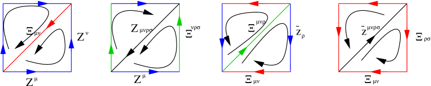
Figure 1: Plaquettes types are , respectively 2-1-1, 4-1-3, 3-2-1 and 4-2-2 following the name of the $p$-cell diagonal that the corresponding superfield is residing. The blue link is link fields $\mathbf{Z}_{\mu},\kern 0.6pt\overline{\kern-0.6ptz\kern-0.6pt}\kern 0.6pt_{\mu}$, red is face diagonal (fermi) multiplet ${\bf\Xi}_{\mu\nu}$, green is cube diagonal ${\bf\Xi}^{\nu\rho\sigma}$, and black is the diagonal piercing the hypercube, $\mathbf{Z}_{\mu\nu\rho\sigma},\kern 0.6pt\overline{\kern-0.6ptz\kern-0.6pt}\kern 0.6pt^{\mu\nu\rho\sigma}$

The second line of Eq. (26) is a signed sum over triangular face plaquettes. It is a face-link-link (2-cell, 1-cell, 1-cell) plaquette, 2-1-1 for short. The bosonic contribution of this term includes the usual twisted Eguchi-Kawai (TEK). This is most easily seen by using the polar decomposition of the complex bosonic matrices and by looking to the angular fluctuations. As the triangular plaquettes are oppositely oriented, the fluxes comes with opposite signs. This is shown in fig.1.

The third line of Eq. (26) is a signed sum of a gauge invariant product of a cube-hypercube-link (or 3-4-1) superfields. The 3-4-1 triangular plaquette has nonvanishing projection to only three faces of the hypercube, hence the deformation parameter is just the sum of these three fluxes.

The penultimate line is a triangular plaquette of face-link-cube multiplets ( or 2-1-3) and finally the last line is a face-hypercube-face (or 2-4-2). These are shown in the last two figures in fig.1. The type 2-1-3 plaquette on a fixed Euclidean time-slice is shown in fig.2. The 2-1-3 plaquette in conjunction with 2-1-1 plaquettes provides further insides and is discussed below.

2.3 An intuitive explanation for the deformations

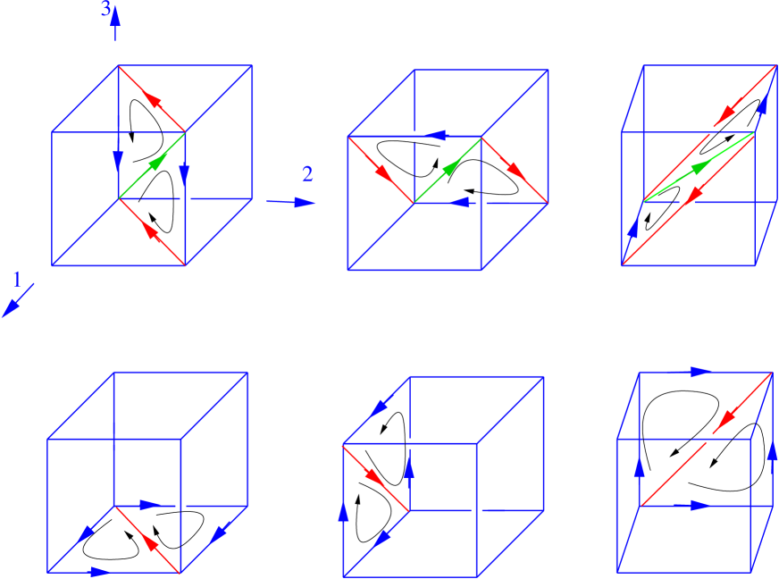
Figure 2: The constant Euclidean time slice of the hypercubic lattice. All possible plaquettes of type 2-3-1 and 2-1-1 are made explicit. The flux through a 2-3-1 is the sum of fluxes passing through its projection on faces. The color coding is same as fig.2.

Consider a fixed Euclidean time slice on the hypercubic lattice, which is a $d=3$ dimensional cubic lattice. The background electric flux $\Phi_{i4}$ is parallel to the $x_{4}=$fixed hypersurface and does not generate a flux for the plaquettes living in that hypersurface. So the deformation of the action in $x_{4}=$ fixed slice will be purely due to magnetic flux $\Phi_{ij}$, where $i,j=1,2,3$. We will show how these fluxes arises by just looking at the orientation and position of the plaquettes in figure.2.

Let us consider the part of the action that lives on the three dimensional hyperspace. The relevant terms in the action are ${\bf\Xi}_{ij}{\bf E}^{ij}|_{\theta}+{\bf\Xi}^{kij}[\kern 0.6pt\overline{\kern-0.6ptz\kern-0.6pt}\kern 0.6pt_{k},{\bf\Xi}_{ij}]$ where ${\bf E}^{ij}=[\mathbf{Z}^{i},\mathbf{Z}^{j}]$. Both are plaquette terms, but of different nature. The first one is the sum of the closed oriented loops on the three faces of the cube. The second one involves the diagonal of the cube which pierces the volume of the cube, a face diagonal, and an ordinary link. These two types are shown in the figure 2. The deformed action is

$${\bf\Xi}_{ij}[e^{-i\Phi_{ij}/2}\mathbf{Z}^{i}\mathbf{Z}^{j}-e^{i\Phi_{ij}/2}\mathbf{Z}^{j}\mathbf{Z}^{i}]|_{\theta}+{\bf\Xi}^{ijk}[e^{-i(\Phi_{ki}+\Phi_{kj})/2}\kern 0.6pt\overline{\kern-0.6ptz\kern-0.6pt}\kern 0.6pt_{k}{\bf\Xi}_{ij}-e^{i(\Phi_{ki}+\Phi_{kj})/2}{\bf\Xi}_{ij}\kern 0.6pt\overline{\kern-0.6ptz\kern-0.6pt}\kern 0.6pt_{k}]\;.$$ (37)

The orientation of the gauge invariant product of superfields (shown in figure 2) determine the sign of the deformation parameter. The relative signs between 2-3-1 and 2-1-1 type plaquettes can also be understood similarly. For example, in figure 2, any of the 2-3-1 type plaquette has nonvanishing projection on two faces and zero projection on the other. However, the orientation of the projected 2-3-1 is opposite of the corresponding 2-1-1 plaquettes. This accounts for the overall difference of the sign among the fluxes between these two types of plaquettes. All the other plaquette terms and deformation parameters in deformed action Eq. (26) can be understood similarly.

3 Noncommutative moduli space

The classical moduli space of vacua is determined by the vanishing of the bosonic action. The bosonic action of the deformed theory, as expressed in Eq. (1), is a sum of the $d$-term and $E$-term. Therefore, the problem at hand reduce to the study of $d$ and $E$-flatness, which is a set of quadratic matrix polynomial equations .

Surprisingly, the zero action configurations of the deformed Type IIB action turns out to be closely related to the TEK action, whose general solutions are well known [7, 28]. This relation is somewhat unexpected since the the bosonic deformed Type IIB action is expressed in terms of ten non-compact, algebra-valued matrices, whereas the TEK is expressed in terms of four group valued unitary matrices. The TEK, for a given nonzero deformation parameter, does not possess a moduli space, but a discrete set of vacua modulo gauge rotations. This discrete set of vacua play an essential role in the description of the moduli space of deformed Type IIB. In the rest of this section we first review the zero action configuration of both EK and TEK, then explore the moduli space of the deformed Type IIB in connection with TEK.

3.1 The relation between TEK and deformed Type IIB

The construction of the deformed Type IIB matrix model, given in appendix A, follows from a dimensional reduction scheme which admits twisted boundary conditions. The reduction by using periodic boundary conditions produces the Type IIB matrix model. This is in essence, the relation between Eguchi-Kawai (EK) model and twisted Eguchi-Kawai (TEK) model.

The EK model is a matrix model of $d$ unitary matrices $U_{\mu}$, obtained by dimensionally reducing the lattice Wilson action to a single point. The action is typically written as

$$S_{EK}=-\beta\sum_{\mu\neq\nu}\operatorname{Tr\,}(U_{\mu}U_{\nu}U_{\mu}^{\dagger}U_{\nu}^{\dagger}-1)+h.c.=\beta\sum_{\mu\neq\nu}\operatorname{Tr\,}|U_{\mu}U_{\nu}-U_{\nu}U_{\mu}|^{2}$$ (38)

Historically, this model had been introduced to work the large $N_{c}$ limit of the gauge theories [29]. It is shown in [29] that the reduced model becomes equivalent to the full theory provided the center symmetry (in the reduced model) is not spontaneously broken. However, this does not happen to be the case at weak coupling (large $\beta$) [30], and there is indeed a remnant of the confinement-deconfinement phase transition at the level of the matrix model. At and above the critical value of the coupling constant $\beta_{c}$, the Polyakov loop acquires a vacuum expectation value. The eigenvalues of the Polyakov loop become nonuniformly distributed, and they clump.(For more recent discussions of TEK in context of large $N_{c}$ equivalences see [31], and in the noncommutative gauge theory context see [32])

The twisted EK is a variant of the EK model, which is introduced to prevent spontaneous symmetry breaking, hence is a cure for the clumping of eigenvalues. (Another solution is quenching [30]) The action is altered in such a way that the eigenvalues of the unitary matrices are uniformly distributed even at the very weak coupling. The TEK action is given by [2]

$$S_{TEK}=-\beta\sum_{\mu\neq\nu}\operatorname{Tr\,}(e^{-i\Phi_{\mu\nu}}U_{\mu}U_{\nu}U_{\mu}^{\dagger}U_{\nu}^{\dagger}-1)+h.c.=\beta\sum_{\mu\neq\nu}\operatorname{Tr\,}|e^{-i\Phi_{\mu\nu}/2}U_{\mu}U_{\nu}-e^{i\Phi_{\mu\nu}/2}U_{\nu}U_{\mu}|^{2}\qquad$$ (39)

where $e^{i\Phi_{\mu\nu}}$ is the flux factor as in Eq. (18). Notice that the TEK action can be thought as a part of the full deformed Type IIB action. This can be done by doing a polar decomposition of the complex matrices as $z_{\mu}=H_{\mu}U_{\mu}$ and looking to a configuration for which the radial modes are proportional to identity, as in [33]. Freezing the radial fluctuations and paying attention to only angular ones yields $\sum_{\mu\neq\nu}|E^{\mu\nu}|^{2}\sim S_{TEK}$, where $E$’s are given in Eq. (36).

The twisting (deformation) in Eq. (39) is an element of ${\mathbb{Z}}_{N_{c}}$ and has an important implication. It forces the eigenvalues of the Polyakov loops to be uniformly distributed even at weak coupling, preventing the Polyakov loops from acquiring vacuum expectation values. The zero action configurations of TEK action are given by

$$U_{\mu}^{0}\,U_{\nu}^{0}=e^{i\Phi_{\mu\nu}}\,U_{\nu}^{0}\,U_{\mu}^{0}$$ (40)

which has well-known twist-eating solutions. These solutions are expressed in terms of clock $P_{L}$ and shift $Q_{L}$ matrices given by $(P_{L})_{jk}=e^{2\pi ik/L}\delta_{jk}$ and $(Q_{L})_{jk}=\delta_{j+1,k}$.

We consider the simplest deformations in $U(N_{c})$ matrix theory corresponding to $n$ units of electric and magnetic flux in z-direction. The flux matrix comes into the canonical form:

$$\Phi_{\mu\nu}=\frac{2\pi n}{N_{c}}1_{2}\otimes i\sigma_{2}$$ (41)

where $1_{2}$ is two dimensional identity and $\sigma_{2}$ is the antisymmetric Pauli matrix. The zero action configuration for $N_{c}=L^{2}$ and $n=L$ background can be written as

$$U_{1}^{0}=P_{L}\otimes 1_{L},\qquad U_{2}^{0}=Q_{L}\otimes 1_{L},\qquad U_{3}^{0}=1_{L}\otimes P_{L},\qquad U_{4}^{0}=1_{L}\otimes Q_{L}$$ (42)

The solution is unique modulo gauge transformations. Its significance for the deformed type IIB will be discussed in depth in the next section, but at this point it is useful to realize that these are generators of a four dimensional (fuzzy) torus.

3.2 The noncommutative moduli space of deformed Type IIB

The zero action configurations of the Eq. (26) are determined by the $d$ and $E$ flatness conditions

$$id=\sum_{m=1}^{5}[\kern 0.6pt\overline{\kern-0.6ptz\kern-0.6pt}\kern 0.6pt^{m},z_{m}]=0,\qquad$$ (43)

$$\kern 0.6pt\overline{\kern-0.6ptE\kern-0.6pt}\kern 0.6pt_{\mu\nu}=\kern 0.6pt\overline{\kern-0.6ptz\kern-0.6pt}\kern 0.6pt_{\mu}\kern 0.6pt\overline{\kern-0.6ptz\kern-0.6pt}\kern 0.6pt_{\nu}-e^{i\Phi_{\mu\nu}}\;\kern 0.6pt\overline{\kern-0.6ptz\kern-0.6pt}\kern 0.6pt_{\nu}\kern 0.6pt\overline{\kern-0.6ptz\kern-0.6pt}\kern 0.6pt_{\mu}=0,$$ (44)

$$\kern 0.6pt\overline{\kern-0.6ptE\kern-0.6pt}\kern 0.6pt_{\mu 5}=\kern 0.6pt\overline{\kern-0.6ptz\kern-0.6pt}\kern 0.6pt_{\mu}\kern 0.6pt\overline{\kern-0.6ptz\kern-0.6pt}\kern 0.6pt_{5}-e^{-i\sum_{\nu\neq\mu}\Phi_{\mu\nu}}\;\kern 0.6pt\overline{\kern-0.6ptz\kern-0.6pt}\kern 0.6pt_{5}\kern 0.6pt\overline{\kern-0.6ptz\kern-0.6pt}\kern 0.6pt_{\mu}=0$$ (45)

which are a total of eleven quadratic matrix polynomial equations. The $d$-flatness condition is unaltered with respect to undeformed case. The matrices satisfying the $E$-flatness condition will also satisfy the $d$-term condition, following the analysis of [34] . Henceforth, our goal is to obtain the solution of the $E=0$.

Let us first recall the moduli space of the (undeformed) Type IIB theory, given by $d$ (as above) and $E$-flatness conditions $E^{mn}=[z^{m},z^{n}]=0$. Solutions are mutually commuting, diagonal matrices with complex eigenvalues. Hence, the moduli space of the matrix model Eq. (12) with gauge group $U({N_{\rm c}})$ is

$${\cal M}={\mathbb{C}}^{5N_{\rm c}}/{S_{N_{\rm c}}}$$ (46)

where ${S_{N_{\rm c}}}$ is the Weyl group of $U({N_{\rm c}})$. This moduli space is a commutative one since the matrices are simultaneously diagonalizable.

We now describe the noncommutative moduli space, given by Eq. (45). The equation in the penultimate line of Eq. (45) is, in fact, the same as the equation for the minima of the twisted EK model Eq. (40), with one essential difference. In TEK, the $U_{\mu}$ matrices are group valued, unitary matrices. Whereas, the $z_{m}$ matrices entering Eq. (45) are noncompact algebra-valued, complex matrices. The solutions of Eq. (40) will satisfy the Eq. (45) as well. Then, the solution of Eq. (45) will be of the form

$$z_{\mu}=c_{\mu}U_{\mu}^{0},\qquad{\rm\,no\,sum}$$ (47)

where $c_{\mu}$ is a complex moduli which is associated with the rigid rotations and overall scaling of the eigenvalues. The equation $E_{\mu 5}=0$ will be satisfied if

$$z_{5}=c_{5}U_{5}^{0}=c_{5}\left(\prod_{\nu=1}^{4}U_{\nu}^{0}\right)^{\dagger}\,,$$ (48)

where $c_{5}$ is an independent complex number. The $z_{5}$, apart from the scale factor $c_{5}$, is not an independent matrix and its form is fixed by the other four $U_{\mu}^{0}$’s.

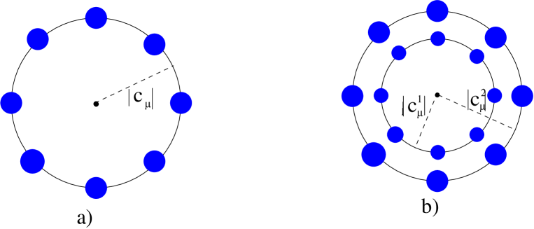
Figure 3: The distribution of eigenvalues of one of the $z_{\mu}$ matrices. The moduli fields corresponds to the rigid rotations of eigenvalues and their overall scaling. a) The $k=1$ case. The target theory has a $U(1)$ gauge group. b) The $k=2$ case. For coinciding $c_{\mu}^{1}$ and $c_{\mu}^{2}$, there is an enhanced gauge symmetry group $U(2)$, otherwise the gauge group is $U(1)\times U(1)$.

The space of the minima of the deformed type IIB action is therefore parametrized by five continuous parameters, $c_{1},\ldots,c_{5}$ and a finite set of unitary matrices satisfying the constraint Eq. (40). The eigenvalues of the twist-eating matrices $U_{m}^{0}$ are roots of unity. The eigenvalues of each $z_{m}$ are uniformly distributed over a circle of radius $c_{\mu}$, see fig.3 a). The modulus and the phase of $c_{m}$ correspond to the overall scaling and the rigid rotation of the eigenvalues, as noted earlier. To be more precise, for $N_{c}=L^{2}$, and flux $n=L$, the eigenvalues of the matrix $z_{m}$ are partitioned into $L$ groups, located at $c_{m}e^{2\pi ik/L}$ where $k=0,\ldots L-1$. For our interpretation of the deformed matrix model as a four dimensional field theory, these moduli modes are essential .

Modulo these five complex numbers, and an extra unitary matrix $U_{5}^{0}$ (which is fixed by the other four $U_{\mu}^{0}$), the set of zero action configurations of the deformed Type IIB matrix model Eq. (45) is same as the one of the corresponding TEK (with the same background flux). We can express the moduli space of the deformed theory as

$${\cal M}_{deformed}={\mathbb{C}}^{5}\times M_{TEK}$$ (49)

Here $M_{TEK}$ corresponds to a finite, discrete set of vacua which happens to coincide with the minima of corresponding TEK Eq. (42) As noted in section 3.1, the procedure to construct $M_{TEK}$ is discussed in depth in literature and books (see for example [35]).

The deformation changes the structure of the classical moduli space drastically , turning the classical commutative moduli space ${\cal M}={\mathbb{C}}^{5N_{\rm c}}/S_{N_{\rm c}}$ in which the eigenvalues can take any value (without increasing the action) to a space in which there are only five free complex parameters. Recalling the polar decomposition of a complex $GL(N_{c},{\mathbb{C}})$ into a product of a Hermitian positive definite matrix and a unitary matrix, $z_{\mu}=H_{\mu}U_{\mu}$, we observe that, in the moduli space of the deformed theory, the radial coordinates are forced to be equal: $H_{\mu}=|c_{\mu}|1_{N_{c}}$. The nonuniformities disrespecting the $\mathbb{Z}_{L}$ in the eigenvalue distribution, in either radial or angular direction, increase the action.

The reader may also wonder if there are other solutions to Eq. (45) and if any, what do they correspond to. There are indeed such solutions and the ones for which at least two out of five $z_{m}$ are zero are of different character. For example, in $z^{1}=z^{2}=0$ case, it is not possible to generate a four dimensional spacetime. As we will see in section 4.1, the main moral of Eq. (47) is that it forms a complete basis for $GL(N_{c},{\mathbb{C}})$ matrices, which in turn becomes the basis for the emergent lattice theory. The case for which at least two out of five matrices is zero a full basis for $GL(N_{c},{\mathbb{C}})$ can not be constructed and we do not obtain a four dimensional target theory. However, it is still possible to obtain a two dimensional target theory. If at least four out of five matrices are zero, then it is not even possible to obtain a two dimensional theory. The technique for the study of the full set of solutions is given in ref.[9], and a similar deformation of the superpotential of ${\cal N}=4$ is worked out there as an example. We refer the reader to ref.[9] for further discussions.

(Ir)reducible Representations

Up to this point, we have discussed the theory with $N_{c}=L^{2}$ and $n=L$, where $\Phi_{\mu\nu}=\frac{2\pi}{L}1_{2}\otimes i\sigma_{2}$. As we will see momentarily, this background supports a $U(1)$ target theory on a four dimensional lattice with $L^{4}$ sites. In order to get a $U(k)$ theory on the same lattice, all we need to do is to take $N_{c}=L^{2}k$ and $n=Lk$. In this case, the moduli space is described by matrices

$$z^{m}=C_{m}\otimes U_{m}^{0},\qquad{\rm where}\qquad C_{m}={\rm Diag}\;(c_{m}^{1},\ldots,c_{m}^{k})$$ (50)

where $C_{m}$ is diagonal $k\times k$ moduli matrix and the solution can be thought as a direct sum of irreducible solutions in the form $\bigoplus_{i=1}^{k}c_{m}^{i}U_{m}=C_{m}\otimes U_{m}^{0}$. Therefore, the moduli space can be expressed as

$${\cal M}_{deformed}={\mathbb{C}}^{5k}/{S_{k}}\otimes M_{TEK}$$ (51)

The four dimensional lattice basis in terms of zero action configurations is encoded into $M_{TEK}$, and will be given explicitly in the next section. We will see how the noncommutativity of the moduli space is tied to the noncommutativity of lattice base space.

Before moving on, we want to make one more observation. Geometrically, the $k=1$ describes the eigenvalues residing on the surface of a four dimensional (fuzzy) hypertorus $T^{4}$. For $k\geq 2$, there are multiple, concentric fuzzy tori $T^{4}$, see fig.3b). When these concentric tori are on top of each other, there is an enhanced gauge symmetry group $U(k)$. If all of them are separated, the gauge group of the lattice theory is $U(1)^{k}$. This phenomena is same as the emergence of $U(k)$ gauge theory on a stack of $k$ D-branes wrapped on a hypertorus. We will comment more on that in section 5.

4 The emergence of (noncommutative) base space

4.1 Fluctuations

In this section, we show that the deformed Type IIB action Eq. (26), without any orbifold constraints whatsoever, is a lattice regularization of ${\cal N}=4$ SYM theory. The emergent lattice is noncommutative. However, depending on the deformation parameter, it is possible to find two continuum limits: one is regular ${\cal N}=4$ SYM, and the other is its noncommutative counterpart.

Let us start with the deformed Type IIB action Eq. (26) with gauge group $U(N_{c})$ where $N_{c}=L^{2}k$ and with the flux matrix $\Phi_{\mu\nu}=\frac{2\pi}{L}(1_{2}\otimes i\sigma_{2})$. In section 3.2, we found the zero action configuration of deformed type IIB. We will analyze the bosonic and fermionic fluctuations around this background. To do that, we decompose the bosonic matrices into fluctuations and background as

$$z^{m}={\widetilde{z}_{m}}U_{m}^{0}\equiv{\widetilde{z}}^{m}D_{m}\qquad{\rm no\;\;sum}$$ (52)

where $U_{m}^{0}$ is a background field configuration and ${\widetilde{z}^{m}}$ are fluctuations around it. The change in naming of the background is due to the physical interpretation, that the $U_{m}^{0}$ will have momentarily, as displacement (discrete translation) operator on the lattice. Substituting Eq. (52) into the bosonic part of the deformed action Eq. (26) yields

$$S_{b}=\frac{\operatorname{Tr\,}}{g^{2}}\left[\frac{1}{2}\Big{(}\sum_{m=1}^{5}[(D_{m}^{\dagger}\widetilde{\kern 0.6pt\overline{\kern-0.6ptz\kern-0.6pt}\kern 0.6pt}_{m}D_{m})(D_{m}^{\dagger}\widetilde{z}^{m}D_{m})-\widetilde{z}^{m}\widetilde{\kern 0.6pt\overline{\kern-0.6ptz\kern-0.6pt}\kern 0.6pt}_{m}]\Big{)}^{2}+\sum_{m,n}|\widetilde{z}^{m}(D_{m}{\widetilde{z}}^{n}D_{m}^{\dagger})-m\leftrightarrow n|^{2}\right]\;\;\;\;$$ (53)

where the phase factors disappeared upon the use of the Eq. (40).

The fluctuations entering the action are $U(N_{c})$ algebra valued and are conventionally expressed as $\widetilde{z}=z^{A}t^{A};\,\,A=1,\ldots N_{c}^{2}$; where $t^{A}$ are Hermitian generators and satisfy the standard commutation relations $[t^{A},t^{B}]=if^{AB}_{{\phantom{AB}}C}\,t^{C}$ . Instead, we will use a basis which makes the mapping of the $N_{c}\times N_{c}$ (where $N_{c}=L^{2}k$) matrix into $U(k)$ fields on $L^{4}$ lattice clearer. We introduce $J_{\bf p}=e^{-i\pi(p_{1}p_{2}+p_{3}p_{4})/L}(U_{2}^{0})^{p_{1}}(U_{1}^{0})^{p_{2}}(U_{4}^{0})^{p_{3}}(U_{3}^{0})^{p_{4}}$, where $p_{\mu}=1,\ldots L$ which form a complete and orthogonal set for $L^{2}\times L^{2}$ matrices, $GL(L^{2},\mathbb{C})$. The $J_{\bf p}$ basis is identifiable as the dual momentum basis for the lattice and p is an integer vector labeling points in Brillouin zone, $\mathbb{Z}_{L}^{4}$. By a Fourier transform, we construct the coordinate basis $\Delta_{{\bf n}}$, where

$$\Delta_{{\bf n}}=\frac{1}{L^{4}}\sum_{{\bf p}\in{\mathbb{Z}}_{L}^{4}}J_{\bf p}e^{2\pi i{\bf p}.{\bf n}/L}$$ (54)

Hence, we can express the map between a $\widetilde{z}$ fluctuation matrix and fields in the $L^{4}$ dual momentum space lattice (or equivalently $L^{4}$ real space lattice ) as

$$\widetilde{z}=\sum_{A=1}^{N_{c}^{2}}z^{A}t^{A}=\sum_{{\bf p}\in{\mathbb{Z}}_{L}^{4}}\sum_{a=1}^{k^{2}}(t^{a}\otimes J_{\bf p}^{\dagger})z_{\bf p}^{a}=\sum_{{\bf p}\in{\mathbb{Z}}_{L}^{4}}z_{\bf p}\otimes J_{\bf p}^{\dagger}\qquad{\rm or}\qquad{\widetilde{z}}=\sum_{{\bf n}\in{\mathbb{Z}}_{L}^{4}}z_{\bf n}\otimes\Delta_{\bf n}$$ (55)

We are essentially expressing a $GL(L^{2}k,{\mathbb{C}})$ matrix by using complementary complete basis matrices, $J_{\bf p}\in GL(L^{2},{\mathbb{C}})$ and $t^{a}\in GL(k,{\mathbb{C}})$. Notice that this representation makes clear how color degrees of freedom of the deformed matrix theory turns into a noncommutative space time in the lattice theory. The properties of the basis matrices are given in [35]. The beauty of this basis is that the zero-action configurations $D_{\mu}\equiv U_{\mu}^{0}$ acts as displacement operator on the position space lattice. Namely,

$$D_{\mu}\left(\Delta_{\bf n}\otimes z_{\bf n}\right)D_{\mu}^{\dagger}=\Delta_{\bf n-\hat{e}_{\mu}}\otimes z_{\bf n}$$ (56)

This relation provides a nearest neighbor interaction on the lattice. By using the orthogonality of basis matrices $J_{\bf p}$ and Eq. (56), the bosonic action can be expressed as

$$S=\frac{\operatorname{Tr\,}}{g^{2}}\sum_{{\bf n}\in{\mathbb{Z}}_{L}^{4}}\left[\frac{1}{2}(\sum_{m}(\kern 0.6pt\overline{\kern-0.6ptz\kern-0.6pt}\kern 0.6pt_{m,\bf{n-\hat{e}_{m}}}\star{z}_{m,\bf{n-\hat{e}_{m}}}-{z}_{m,\bf n}\star\kern 0.6pt\overline{\kern-0.6ptz\kern-0.6pt}\kern 0.6pt_{m,\bf n}))^{2}+\sum_{m,n}|({z}_{m,\bf n}\star{z}_{n,\bf{n+\hat{e}_{m}}}-m\leftrightarrow n|^{2}\right]\qquad$$ (57)

This is indeed just the noncommutative generalization of bosonic part of Eq. (8). Performing the same analysis at the level of superfields, it is easy to show that the deformed Type IIB action Eq. (26) may be rewritten as

$$S = \frac{\operatorname{Tr\,}}{g^{2}}\sum_{\bf n}\int\;d\theta\bigg{(}-\frac{1}{2}{\bf\Lambda_{\bf n}}\star{\partial}_{\theta}{\bf\Lambda_{\bf n}}-{\bf\Lambda_{\bf n}}\star(\kern 0.6pt\overline{\kern-0.6ptz\kern-0.6pt}\kern 0.6pt_{m,\bf{n-\hat{e}_{m}}}\star{\bf Z}_{m,\bf{n-\hat{e}_{m}}}-{\bf Z}_{m,\bf n}\star\kern 0.6pt\overline{\kern-0.6ptz\kern-0.6pt}\kern 0.6pt_{m,\bf n})\bigg{.}$$ (61)

$$\bigg{.}+\frac{1}{2}{\bf\Xi}_{\mu\nu,\bf n}\star({\bf Z}_{\mu,\bf n}\star{\bf Z}_{\nu,\bf{n+\hat{e}_{\mu}}}-{\bf Z}_{\nu,\bf n}\star{\bf Z}_{\mu,\bf{n+\hat{e}_{\nu}}})+{\bf\Xi}_{\mu 5,\bf n}\star({\bf Z}_{\mu,\bf n}\star{\bf Z}_{5,\bf{n+\hat{e}_{\mu}}}-{\bf Z}_{5,\bf n}\star{\bf Z}_{\mu,\bf{n+\hat{e}_{5}}})\bigg{)}$$

$$+\frac{\sqrt{2}}{2}\epsilon^{\mu\nu\rho\sigma}{\bf\Xi}_{\mu\nu,\bf n}\star(\kern 0.6pt\overline{\kern-0.6ptz\kern-0.6pt}\kern 0.6pt_{\rho,\bf{n-\hat{e}_{\rho}}}\star{\bf\Xi}_{\sigma 5,\bf{n+\hat{e}_{\mu}+\hat{e}_{\nu}}}-{\bf\Xi}_{\sigma 5,\bf{n-\hat{e}_{\sigma}-\hat{e}_{5}}}\star\kern 0.6pt\overline{\kern-0.6ptz\kern-0.6pt}\kern 0.6pt_{\rho,\bf{n+\hat{e}_{\mu}+\hat{e}_{\nu}}})$$

$$+\frac{\sqrt{2}}{8}\epsilon^{\mu\nu\rho\sigma}{\bf\Xi}_{\mu\nu,\bf n}\star(\kern 0.6pt\overline{\kern-0.6ptz\kern-0.6pt}\kern 0.6pt_{5,\bf{n-\hat{e}_{5}}}\star{\bf\Xi}_{\rho\sigma,\bf{n+\hat{e}_{\mu}+\hat{e}_{\nu}}}-{\bf\Xi}_{\rho\sigma,\bf{n-\hat{e}_{\rho}-\hat{e}_{\sigma}}}\star\kern 0.6pt\overline{\kern-0.6ptz\kern-0.6pt}\kern 0.6pt_{5,\bf{n+\hat{e}_{\mu}+\hat{e}_{\nu}}})$$

The lattice star product is defined by

$$\Psi_{1,{\bf n}}\star\Psi_{2,{\bf n}}=\frac{1}{L^{4}}\sum_{{\bf j},{\bf k}}\Psi_{1,{\bf j}}\;\Psi_{2,{\bf k}}\;\;e^{-\frac{4\pi i}{L^{2}\theta^{\prime}}\;({\bf j}-{\bf n})\wedge({\bf k}-{\bf n})}$$ (62)

which is a non-local product and $\theta^{\prime}=2/L$ is a dimensionless noncommutativity parameter on the lattice.

4.2 Classical spectrum

The action Eq. (61) has no explicit lattice spacing, but it has a classical moduli space for which the bosonic lattice action vanishes. The distance from the origin of the moduli space is identified as inverse lattice spacing, and hence the continuum limit is defined as a trajectory out to infinity in the moduli space.

The zero action configuration of the lattice corresponds to site independent diagonal matrices $z_{m,{\bf n}}=C_{m}={\rm Diag}\;(c_{m}^{1},\ldots,c_{m}^{k})$, hence the moduli space is given by ${\cal M}=\mathbb{C}^{5k}/S_{k}$. Notice that this is (and has to be) the moduli space of the deformed Type IIB action, as Eq. (61) is merely a rewriting.

We expand the action around a $U(k)$ gauge symmetry preserving, hypercubic spacetime lattice point:

$$z^{\mu}_{{\bf n}}=\kern 0.6pt\overline{\kern-0.6ptz\kern-0.6pt}\kern 0.6pt_{\mu,{\bf n}}=\frac{1}{\sqrt{2}a}1_{k},\qquad z^{5}_{{\bf n}}=\kern 0.6pt\overline{\kern-0.6ptz\kern-0.6pt}\kern 0.6pt_{5,{\bf n}}=0$$ (63)

We use a cartesian decomposition of the bosonic matrices around the point Eq. (63) as

$$z_{\mu,{\bf n}}=\frac{1}{\sqrt{2}a}1_{k}+\frac{S_{\mu,{\bf n}}+iV_{\mu,{\bf n}}}{\sqrt{2}},\qquad z_{5,{\bf n}}=\frac{S_{5,{\bf n}}+iS_{6,{\bf n}}}{\sqrt{2}}$$ (64)

where $S$ and $V$ are identified as six scalars and four gauge bosons of the target ${\cal N}=4$ supersymmetric Yang-Mills theory.

The classical spectrum can be found by diagonalizing the kinetic terms, similar to the appendix B in [4]. This can be done by introducing the Fourier transform of a field $\Psi_{{\bf n}}$

$$\Psi_{{\bf n}}=\frac{1}{L^{2}}\sum_{{\bf p}\in B.Z.}e^{i{\bf p.n}a}\Psi_{{\bf p}}$$ (65)

where the $p_{\mu}=\frac{2\pi}{La}{\hat{p}}_{\mu}\in[-\pi/a,\pi/a)$ is discrete momenta in hypercubic Brillouin zone (B.Z.), and ${\hat{p}}_{\mu}$ is integer in the range $[-L/2,L/2)$. This diagonalize the kinetic terms for the bosonic action

$$\frac{\operatorname{Tr\,}}{2g^{2}}\sum_{{\bf p}\in B.Z.}\big{[}\sum_{a=1}^{6}S_{a,{\bf p}}M_{\bf p}^{2}S_{a,{-\bf p}}+V_{\mu,{\bf p}}G_{\mu\nu,{\bf p}}V_{\nu,-{\bf p}}\big{]}$$ (66)

where we define

$${{\cal P}}_{\mu}\equiv\frac{2}{a}\sin\;\frac{ap_{\mu}}{2}\,,\qquad M_{\bf p}^{2}=\sum_{\mu=1}^{4}{{\cal P}}_{\mu}^{2}\,,\;\qquad\;G_{\mu\nu,{\bf p}}=M_{\bf p}^{2}\delta_{\mu\nu}-{{\cal P}}_{\mu}{{\cal P}}_{\nu}e^{-ia(p_{\mu}-p_{\nu})/2}\qquad$$ (67)

The six scalars are degenerate for a given momenta and have eigenvalue $M_{\bf p}^{2}$. The eigenvalues for the gauge boson matrix $G_{\mu\nu,{\bf p}}$ are a three fold degenerate $M_{\bf p}^{2}$ and zero. The zero mode of $G$ is the consequence of gauge invariance. The essential point here is the absence of doublers in the bosonic spectrum, $M_{\bf p}^{2}$, which is only zero at the origin of the Brillouin zone and which reaches its maximum at the corners. The exact supersymmetry implies there are no fermion doublers either (see [12] for an explicit analysis.) The absence of the fermionic doublers is also a consequence of associating the sixteen fermions with the $p$-cells of the lattice (see [24]). . In the continuum limit, which is defined by

$$a\rightarrow 0,\;\;\;L\rightarrow\infty,\;\;\;La={\rm fixed},$$ (68)

we obtain ${{\cal P}}_{\mu}\rightarrow p_{\mu}$ and $M_{\bf p}^{2}\rightarrow p^{2}$ and $G_{\mu\nu,{\bf p}}\rightarrow(p^{2}\delta_{\mu\nu}-p_{\mu}p_{\nu})$ correctly reproducing the kinetic terms of bosonic action.

Moduli space: A second pass

We reconsider the eigenvalue distribution shown in fig.3 and make various observations. For simplicity, consider the case $k=1$. In finding the spectrum, we expand the fields around the point Eq. (63) in moduli space. This means setting $c_{\mu}=\frac{1}{a}$ and $c_{5}=0$, where $a$ is interpreted as the lattice spacing. Turning on $c_{5}$ is related to deforming the hypercubic lattice to the $A_{4}^{*}$ lattice and tilting the $T^{4}$, and we ignore this possibility for simplicity. Consider the eigenvalue distribution on the circle shown in fig.3, which is one of the directions on fuzzy $T^{4}$ on which eigenvalues are distributed. The circumference of the circle is

$$2\pi c_{\mu}=\frac{2\pi}{a}$$ (69)

which is, in fact, the extent of the Brillouin zone in the $\mu$ direction. The separation between two nearest-neighbor in moduli space along the circle (geodesic distance on the torus) is given by $2\pi c_{\mu}/L=\frac{2\pi}{La}$ and this corresponds to the minimal lattice momenta. The geodesic separation between two eigenvalues separated by $\hat{p}_{\mu}\in[-L/2,L/2)$ units is given by $p_{\mu}=\frac{2\pi}{Na}\hat{p}_{\mu}\in[-\pi/a,\pi/a)$ and is the discrete momenta in Brillouin zone of hypercubic lattice. As a last remark, notice that the external distance between the same two points as above is $\frac{2}{a}\sin\frac{ap_{\mu}}{2}$, the acoustic phonon spectrum in one dimension. The continuum limit is taken as a trajectory out to infinity in moduli space, by keeping the volume and four dimensional coupling constant fixed. Hence, the circumference of eigenvalue circle in moduli space (and extent of the Brillouin zone) becomes $p_{\mu}\in[-\pi/a,\pi/a)\rightarrow[-\infty,\infty)$. It seems natural to interpret the four dimensional torus that the eigenvalues reside as the Brillouin zone, and the action as the momentum space action, with momenta summed over the Brillouin zone.

In the derivation of Eq. (61), we used a Fourier transform, which took us from momentum space representation ($J_{\bf p}$) of the lattice to the position space representation ($\Delta_{{\bf n}}$). Hence, the inverse extend of Brillouin zone (divided by $2\pi$ ) becomes the UV cutoff. The inverse of minimal momenta (divided by $2\pi$) becomes the IR cutoff ($La$), the size of the spacetime torus. The four dimensional target field theory lives on this spacetime torus, whose extent remains fixed as we take the continuum limit. It should be emphasized that the target space is not the space that the eigenvalues reside, but its Fourier transform.

4.3 Localization of interactions

In this subsection, we will describe the circumstances under which the non-locality in Eq. (61) disappears and the interaction becomes local in spacetime. Upon that, the continuum limit of the action becomes the same as the continuum limit of Eq. (8) and reproduces the ${\cal N}=4$ SYM in four dimensions. Since the calculations are very similar to [4], they will not be duplicated here. At the end, we also comment briefly on the non-commutative spacetime limit.

The interaction terms of the lattice action Eq. (61) are non-local, involving a sum over all lattice points. In the continuum limit, the star-product becomes

$$\Psi_{1}({\bf w})\star\Psi_{2}({\bf w})=\int d^{4}x\;d^{4}y\;\Psi_{1}({\bf x})K({\bf x}-{\bf w},{\bf y}-{\bf w})\Psi_{2}({\bf y})\;.$$ (70)

The kernel of the integral is

$$K({\bf x}-{\bf w},{\bf y}-{\bf w})=\frac{1}{\pi^{2}\det\Theta}e^{-2i({\bf x}-{\bf w})_{\mu}(\Theta^{-1})^{\mu\nu}({\bf y}-{\bf w})_{\nu}}$$ (71)

and the dimensionful noncommutativity parameter is given by

$$\Theta_{\mu\nu}=\frac{L^{2}a^{2}\theta^{\prime}}{2\pi}(1_{2}\times i\sigma_{2})_{\mu\nu}.$$ (72)

Let us consider the continuum limits in which the volume of the target space is kept fixed. The length scale associated with noncommutativity is the square root of $\Theta_{12}$, denoted as $\sqrt{\Theta}$ for short. Then, for $\sqrt{\Theta}/(La)\rightarrow 0$, i.e, the limit at which noncommutativity goes to zero, the kernel localizes sharply and becomes a Dirac delta function:

$$K({\bf x}-{\bf w},{\bf y}-{\bf w})\rightarrow\delta({\bf x}-{\bf w})\delta({\bf y}-{\bf w}),$$ (73)

yielding a local product out of the star product. From the spacetime point of view, trading the nonlocality of the product of functions back to spacetime noncommutativity, this limit yields a commutative spacetime. This is certainly an interesting limit as it reproduces the ordinary ${\cal N}=4$ SYM target theory.

Explicit calculation shows that, in the continuum limit, we obtain the action of ${\cal N}=4$ SYM at tree level.

$$S=\frac{1}{g_{4}^{2}}\,\int d^{4}x\operatorname{Tr\,}\Bigl{(}\frac{1}{4}V_{\mu\nu}V_{\mu\nu}+\frac{1}{2}(D_{\mu}S_{a})^{2}-\frac{1}{4}\left[S_{a},S_{b}\right]^{2}+\frac{1}{2}\omega^{T}\,C\,(D_{\mu}\,\tilde{\Gamma}_{\mu}\,\omega+i\tilde{\Gamma}_{4+a}\,[S_{a},\,\omega])\Bigr{)}\qquad$$ (74)

where $D_{\mu}=\partial_{\mu}+i[V_{\mu},\cdot\;]$ is the covariant derivative and $V_{\mu\nu}=-i[D_{\mu},D_{\nu}]$ is the nonabelian field strength. The $SO(10)$ gamma matrices ${\tilde{\Gamma}}_{\alpha}$ are basically a reshuffling of the gamma matrix basis introduced in Eq. (2). They are given as ${\tilde{\Gamma}}_{\mu}=\Gamma_{\mu},\;{\tilde{\Gamma}}_{4+m}=\Gamma_{5+m},\;{\tilde{\Gamma}}_{10}=\Gamma_{5}$, following the conventions of section 2.2 of [4]. The charge conjugation matrix $C$ is unchanged with respect to Eq. (2).

Even though the deformed type IIB theory Eq. (26) , hence lattice theory Eq. (61), possesses only ${\cal Q}=1$ exact supersymmetry and a $U(1)^{5}$ global symmetry, the target theory has full ${\cal Q}=16$ supersymmetries and manifest Lorentz invariance along with a global $SO(6)$ R-symmetry.

We believe it is also possible to obtain a lattice action and its continuum for the product gauge group $\prod_{i}U(k_{i})$ where $\sum_{i}k_{i}=k$ by expanding around a point in the moduli space given by $\langle z^{\mu}_{{\bf n}}\rangle=\frac{1}{\sqrt{2}a}1_{k}+(\oplus_{i}c_{i}1_{k_{i}})$. In the continuum limit, we take the lattice spacing to zero by keeping $c_{i}$’s fixed, which produce a $\prod_{i}U(k_{i})$ gauge theory. It is desirable to know whether one can obtain a lattice or matrix regularization for orthogonal and symplectic gauge groups by either performing an orientifold projection on the orbifold lattice or (deformed) type IIB matrix model (The symplectic type IIB is discussed in [36]). Such constructions may be useful in nonperturbative study of electric-magnetic duality [37].

Noncommutative continuum limit

We believe it is also possible to obtain the noncommutative continuum ${\cal N}=4$ theory with the appropriate choices of the background flux matrix $\Phi_{\mu\nu}$, and hence appropriate zero action configurations $U_{\mu}^{0}$, for example the ones given in [16]. In order to achieve this limit, one needs to take $\theta^{\prime}$ fixed (hence $\Theta$ fixed) along with a fixed finite volume. In this case, there is a nonlocality of order $\sqrt{\Theta}$ in the star product of the continuum theory. At distances longer then $\sqrt{\Theta}$, the interactions effectively shuts off because of the fast oscillation of the kernel. The action of the noncommutative ${\cal N}=4$ SYM target theory can be obtained by replacing the product of fields in Eq. (74) by nonlocal continuum star product given in Eq. (70).

5 Collective excitations of D(-1) branes as D3 branes

The results obtained within this paper can be interpreted within the string theory framework. In order to do that, we need to specify the world-volume theories of the corresponding D-brane configurations. The type IIB matrix theory Eq. (2) describes the dynamics of a cluster of D(-1)-branes (which are sometimes referred as D-instantons). These are points in ten dimensional Euclidean space. In this sense a Dp-brane is a p+1 (Euclidean) dimensional hypersurface. The main result of this paper may be interpreted as follows: Upon deforming the type IIB matrix theory, a particular collective excitation of D(-1)-branes becomes the classical vacuum state of the theory. Essentially, the D(-1) branes, instead of being at some random points on the moduli space of the undeformed theory, lie on the surface of a four dimensional torus $T^{4}$. Analyzing the fluctuations around this D(-1) background yields ${\cal N}=4$ supersymmetric Yang-Mills theory, which is the world-volume theory of a collection of D3-branes. Hence the D3-brane, which is not present in the fundamental description of the theory, may be considered as an emergent brane. In the rest of this section, we will describe these statement in a little bit more detail.

The type IIB action Eq. (2) (or Eq. (12)) with gauge group $U(N_{c})$ describes a collection of $N_{c}$ D(-1)-branes (see for example [38]). This theory possess ${\cal Q}=16$ supersymmetries and a global $SO(10)$ symmetry. In the latter form of the action Eq. (12), only the $SU(5)\times U(1)$ subgroup of $SO(10)$ is manifest. The commutative moduli space is (locally) $\mathbb{R}^{10N_{\rm c}}$ (or equivalently ${\mathbb{C}}^{5N_{\rm c}}$). The eigenvalues of these matrices ($v_{\alpha}$ or $z^{m}$) are identified as position of D(-1) branes. In this framework, the D-branes are pointlike objects on the moduli space.

The deformed Type IIB action Eq. (26) is a supersymmetric deformation respectful to a global $U(1)^{5}$ symmetry and ${\cal Q}=1$ supersymmetry. The deformation renders the moduli space (defined by $E$ and d-flatness conditions given in Eq. (45)) a noncommutative one, and forces the eigenvalues of $z_{m}$ matrices (the D(-1) branes) to be uniformly distributed on a circle as in 3. However, as the matrices $z_{1},\ldots z_{5}$ are not simultaneously diagonalizable, the positions of the D(-1) branes are indeterminate and they lie on the surface of a fuzzy four dimensional torus. The classical zero action configuration, given in Eq. (47) and Eq. (48), is a collective excitation of D(-1)-branes and is responsible for the emergence of higher dimensional branes out of the deformed Type IIB matrix theory. Also notice that, the base space of the target theory is not the space that the eigenvalues reside, but the dual space obtained by Fourier transform Eq. (54) in section 4.1. The continuum limit is taken by keeping the size of this dual space fixed. This is similar to the Seiberg-Witten limit where the open string metric and coupling constant rather then the closed string parameters are kept fixed [39] (also see [40, 10]).

It is also reasonable to ask which supergravity field or type IIB string theory field may be responsible for this excitation of D(-1) branes. To answer this question, let us first recall that the world-volume of a Dp-brane couples to a (p+1) form potential $A^{(p+1)}$, given in the form $\int_{Dp}A^{(p+1)}$,or explicitly as $\int A^{\mu_{1}\ldots\mu_{p+1}}\frac{dx_{\mu_{1}}}{d\sigma_{i_{1}}}\ldots\frac{dx_{\mu_{p+1}}}{d\sigma_{i_{p+1}}}\epsilon^{i_{1}\ldots i_{p+1}}d^{p+1}\sigma$, where $x_{\mu}$ are world-sheet coordinates and the integration is over the world-sheet of Dp-brane. The D(-1) branes, whose world-sheet is zero dimensional, couples to a zero form. The configuration we consider above carries $N_{c}$ units of D(-1)-brane charge. Moreover, the fact that the matrices $z_{m}$ do not commute with each other can be interpreted as the existence of higher dimensional branes in the system (see [22] for a review). In our case, the emergent higher dimensional branes are $k$ D3-branes wrapped on a four dimensional spacetime hypertorus, where $k$ is associated with the rank of the gauge group $U(k)$ of the target theory. It is, therefore, tempting to think that the deformations introduced in Eq. (26) on the matrix theory side corresponds to turning on the RR five-form self dual field strength $F^{(5)}$ on the type IIB string theory. The $F^{(5)}$ arises from a four-form field $A^{(4)}$, which, as noted above, couples to D3-branes. The emergence of D3 branes can be thought as a special case of the dielectric brane effect introduced by Myers, which is analogous to polarization of a neutral atoms in an electric field [41]. Similarly, the collective state of D(-1) branes can be thought of as analogous to the emergence of a dipole upon the application of $F^{(5)}$ field. However, the argument we have given here is incomplete as it does not specify the geometry or topology of the emergent object. For example, if we were to construct the analog of ${\cal N}=1^{*}$ theory in four dimension [42], i.e, a mass deformed matrix theory [43], the emergent brane would be a (euclidean) D1 brane wrapped on a two sphere $S^{2}$, whereas the deformation discussed in footnote 8 gives a D1 wrapped on a two torus $T^{2}$. Both of these can be thought as polarization of D(-1) branes. The difference is similar to the emergence of dipole or quadrupole moments upon the application of appropriate electric fields. Certainly, the string theory realization of the deformations warrants further study.

It is also possible to recover the known membranes constructions appearing in Type IIB matrix theory from the large $N_{c}$ limits of our formulation. Let us recall the zero action configurations $z_{\mu}=c_{\mu}U_{\mu}^{(0)}$ and restrict our attention to the small fluctuations of the $U_{\mu}^{(0)}$, and small $\Phi_{\mu\nu}$. Then the conditions describing the vacua $U_{\mu}^{(0)}U_{\nu}^{(0)}=e^{i\Phi_{\mu\nu}}U_{\nu}^{(0)}U_{\mu}^{(0)}$ become $[X_{\mu},X_{\nu}]=-i\Phi_{\mu\nu}$, which describes (locally) a planar membrane, where $X_{\mu}$ are the fluctuations. The latter equation does not admit a solution in terms of finite matrices, and is usually considered to be associated with the existence of a D(p+2) in a system of Dp branes. However, notice that such a configuration is not stable within the Type IIB, but its decay is is suppressed in the large $N_{c}$ [23]. The zero action configurations of the deformed type IIB, on the other hand, admit solutions in terms of finite dimensional matrices, and, more importantly, are stable (This point is also emphasized by Dorey [10]). It is also worth mentioning that the analogs of a planar membrane, in the notation of Eq. (26), is a Fayet-Illiopoulis term, given in the form of a d-term deformation $\zeta\operatorname{Tr\,}\int d\theta\;\bm{\Lambda}=-\zeta\,d$, where $\zeta$ is the deformation parameter. This alters the d-flatness condition into $\sum_{m=1}^{5}[\kern 0.6pt\overline{\kern-0.6ptz\kern-0.6pt}\kern 0.6pt_{m},z^{m}]-\zeta=0$ which only admits solution in terms of infinite dimensional matrices.

Appendix A Derivation of deformed type IIB action

In this appendix we show that the dimensional reduction of the lattice action Eq. (8) to one site model, by using the twisted boundary conditions Eq. (17), gives the deformed type IIB action Eq. (26). We will first perform the reduction. However, this will produce some extraneous gauge rotation matrices, which we will get rid of by appropriate field redefinitions.

The first two term in action Eq. (8) reduce to a form

$$\operatorname{Tr\,}\left[-\frac{1}{2}{\bf\Lambda}{\partial}_{\theta}{\bf\Lambda}-{\bf\Lambda}[(g_{m}^{\dagger}\kern 0.6pt\overline{\kern-0.6ptz\kern-0.6pt}\kern 0.6pt_{m}),({\bf Z}_{m}g_{m})]\right]_{\theta}$$ (75)

which has no flux terms. This is due to the fact that the interaction of site fields with the link fields does not surround an area.

Next, we consider the interactions of fermi multiplets ${\bf\Xi}_{mn}$ with holomorphic ${\bf E}^{mn}$ function. First, notice that the $\theta$ component of the ${\bf\Xi}_{mn}$ fermi multiplet is a composite field, and upon reduction it becomes

$$\kern 0.6pt\overline{\kern-0.6ptz\kern-0.6pt}\kern 0.6pt_{m,{\bf n}+{\bf\hat{e}_{n}}}\kern 0.6pt\overline{\kern-0.6ptz\kern-0.6pt}\kern 0.6pt_{n,{\bf n}}-\kern 0.6pt\overline{\kern-0.6ptz\kern-0.6pt}\kern 0.6pt_{n,{\bf n}+{\bf\hat{e}_{m}}}\kern 0.6pt\overline{\kern-0.6ptz\kern-0.6pt}\kern 0.6pt_{m,{\bf n}}\rightarrow(g_{n}\kern 0.6pt\overline{\kern-0.6ptz\kern-0.6pt}\kern 0.6pt_{m}g_{n}^{\dagger})\kern 0.6pt\overline{\kern-0.6ptz\kern-0.6pt}\kern 0.6pt_{n}-(g_{m}\kern 0.6pt\overline{\kern-0.6ptz\kern-0.6pt}\kern 0.6pt_{n}g_{m}^{\dagger})\kern 0.6pt\overline{\kern-0.6ptz\kern-0.6pt}\kern 0.6pt_{m}$$ (76)

$$=g_{n}g_{m}(g_{m}^{\dagger}\kern 0.6pt\overline{\kern-0.6ptz\kern-0.6pt}\kern 0.6pt_{m})(g_{n}^{\dagger}\kern 0.6pt\overline{\kern-0.6ptz\kern-0.6pt}\kern 0.6pt_{n})-g_{m}g_{n}(g_{n}^{\dagger}\kern 0.6pt\overline{\kern-0.6ptz\kern-0.6pt}\kern 0.6pt_{n})(g_{m}^{\dagger}\kern 0.6pt\overline{\kern-0.6ptz\kern-0.6pt}\kern 0.6pt_{m})=g_{m}g_{n}\left(e^{-i\Phi_{mn}}(g_{m}^{\dagger}\kern 0.6pt\overline{\kern-0.6ptz\kern-0.6pt}\kern 0.6pt_{m})(g_{n}^{\dagger}\kern 0.6pt\overline{\kern-0.6ptz\kern-0.6pt}\kern 0.6pt_{n})-(g_{n}^{\dagger}\kern 0.6pt\overline{\kern-0.6ptz\kern-0.6pt}\kern 0.6pt_{n})(g_{m}^{\dagger}\kern 0.6pt\overline{\kern-0.6ptz\kern-0.6pt}\kern 0.6pt_{m})\right)\qquad$$ (77)

where we used ’t Hooft algebra. Hence the third term in the action becomes

$$\operatorname{Tr\,}\left[{\bf\Xi}_{mn,{\bf n}}\,{\bf E}^{mn}_{{\bf n}}\right]_{\theta}\rightarrow\operatorname{Tr\,}\left[(g_{n}^{\dagger}g_{m}^{\dagger}{\bf\Xi}_{mn})[\;(\mathbf{Z}^{m}g_{m})(\mathbf{Z}^{n}g_{n})-e^{i\Phi_{mn}}\;(\mathbf{Z}^{n}g_{n})(\mathbf{Z}^{m}g_{m})]\right]_{\theta}$$ (78)

Even though we combined the two terms ${\bf\Xi}_{\mu\nu}{\bf E}^{\mu\nu}+2{\bf\Xi}_{\mu 5}{\bf E}^{\mu 5}$ into ${\bf\Xi}_{mn}{\bf E}^{mn}$, these are plaquettes of different types, namely a 2-1-1 and 4-1-3 types (see fig.1).

We are done with the $Q$-exact part of the lattice action. The $Q$-closed part of action includes plaquettes of two types. One is 4-2-2 type, shown in fig.1 and the other is 3-1-2 type shown in fig.1 and more explicitly, in fig.2. The first type involves triangular loops composed of the 4-cell link field and two 2-cell fermionic links. The second type involves a 3-cell fermionic link, a 2-cell fermionic link and a bosonic 1-cell link field. Let us first consider the first type and its reduction. Using the action Eq. (8) and setting $p=5$, we obtain

$$\frac{\sqrt{2}}{8}\epsilon^{\mu\nu\rho\sigma}{\bf\Xi}_{\mu\nu,\bf n}(\kern 0.6pt\overline{\kern-0.6ptz\kern-0.6pt}\kern 0.6pt_{5,\bf{n-\hat{e}_{5}}}{\bf\Xi}_{\rho\sigma,\bf{n+\hat{e}_{\mu}+\hat{e}_{\nu}}}-{\bf\Xi}_{\rho\sigma,\bf{n-\hat{e}_{\rho}-\hat{e}_{\sigma}}}\kern 0.6pt\overline{\kern-0.6ptz\kern-0.6pt}\kern 0.6pt_{5,\bf{n+\hat{e}_{\mu}+\hat{e}_{\nu}}})\rightarrow$$ (79)

$$\frac{\sqrt{2}}{8}\epsilon^{\mu\nu\rho\sigma}{\bf\Xi}_{\mu\nu}((g_{5}^{\dagger}\kern 0.6pt\overline{\kern-0.6ptz\kern-0.6pt}\kern 0.6pt_{5}g_{5})(g_{\mu}g_{\nu}{\bf\Xi}_{\rho\sigma}g_{\nu}^{\dagger}g_{\mu}^{\dagger})-(g_{\sigma}^{\dagger}g_{\rho}^{\dagger}{\bf\Xi}_{\rho\sigma}g_{\rho}g_{\sigma})(g_{\mu}g_{\nu}\kern 0.6pt\overline{\kern-0.6ptz\kern-0.6pt}\kern 0.6pt_{5}g_{\nu}^{\dagger}g_{\mu}^{\dagger}))$$ (80)

$$\frac{\sqrt{2}}{8}\epsilon^{\mu\nu\rho\sigma}(g_{\nu}^{\dagger}g_{\mu}^{\dagger}{\bf\Xi}_{\mu\nu})\left((g_{5}^{\dagger}\kern 0.6pt\overline{\kern-0.6ptz\kern-0.6pt}\kern 0.6pt_{5})\,(g_{5}g_{\mu}g_{\nu}g_{\rho}g_{\sigma})\,(g_{\sigma}^{\dagger}g_{\rho}^{\dagger}{\bf\Xi}_{\rho\sigma})-(g_{\sigma}^{\dagger}g_{\rho}^{\dagger}{\bf\Xi}_{\rho\sigma})(g_{\rho}g_{\sigma}g_{\mu}g_{\nu}g_{5})(g_{5}^{\dagger}\kern 0.6pt\overline{\kern-0.6ptz\kern-0.6pt}\kern 0.6pt_{5})\right)\qquad$$ (81)

In this expression, since the combination $(g_{5}g_{\mu}g_{\nu}g_{\rho}g_{\sigma})\equiv R_{\mu\nu\rho\sigma}$ appears with $\epsilon^{\mu\nu\rho\sigma}$ tensor, with the use of the definition of $g_{5}$ Eq. (17), we see that it is proportional to the identity matrix and can be pulled out of the parenthesis. By using the ’t Hooft’s algebra Eq. (18) in the reordering of the second term, we express Eq. (81) in a simpler form as

$$\frac{\sqrt{2}}{8}\epsilon^{\mu\nu\rho\sigma}R_{\mu\nu\rho\sigma}(g_{\nu}^{\dagger}g_{\mu}^{\dagger}{\bf\Xi}_{\mu\nu})\left((g_{5}^{\dagger}\kern 0.6pt\overline{\kern-0.6ptz\kern-0.6pt}\kern 0.6pt_{5})\,\,(g_{\sigma}^{\dagger}g_{\rho}^{\dagger}{\bf\Xi}_{\rho\sigma})-e^{i(\Phi_{\rho\mu}+\Phi_{\rho\nu}+\Phi_{\sigma\mu}+\Phi_{\sigma\nu})}(g_{\sigma}^{\dagger}g_{\rho}^{\dagger}{\bf\Xi}_{\rho\sigma})(g_{5}^{\dagger}\kern 0.6pt\overline{\kern-0.6ptz\kern-0.6pt}\kern 0.6pt_{5})\right)$$ (82)

where the exponent is a sum of the fluxes passing through all surfaces but $\mu\nu$ and $\rho\sigma$.

The 3-1-2 type plaquettes in $S_{closed}$ can be obtained by setting $p\neq 5$ in Eq. (8). Following very similar steps to the reduction performed above, we obtain

$$4\frac{\sqrt{2}}{8}\epsilon^{\mu\nu\rho\sigma}{\bf\Xi}_{\mu\nu,\bf n}(\kern 0.6pt\overline{\kern-0.6ptz\kern-0.6pt}\kern 0.6pt_{\rho,\bf{n-\hat{e}_{\rho}}}{\bf\Xi}_{\sigma 5,\bf{n+\hat{e}_{\mu}+\hat{e}_{\nu}}}-{\bf\Xi}_{\sigma 5,\bf{n-\hat{e}_{\sigma}-\hat{e}_{5}}}\kern 0.6pt\overline{\kern-0.6ptz\kern-0.6pt}\kern 0.6pt_{\rho,\bf{n+\hat{e}_{\mu}+\hat{e}_{\nu}}})\rightarrow$$ (83)

$$\frac{\sqrt{2}}{2}\epsilon^{\mu\nu\rho\sigma}R_{\mu\nu\rho\sigma}(g_{\nu}^{\dagger}g_{\mu}^{\dagger}{\bf\Xi}_{\mu\nu})\left((g_{\rho}^{\dagger}\kern 0.6pt\overline{\kern-0.6ptz\kern-0.6pt}\kern 0.6pt_{\rho})\;(g_{5}^{\dagger}g_{\sigma}^{\dagger}{\bf\Xi}_{\sigma 5})e^{i(\Phi_{\rho\mu}+\Phi_{\rho\nu})}-(g_{5}^{\dagger}g_{\sigma}^{\dagger}{\bf\Xi}_{\sigma 5})(g_{\rho}^{\dagger}\kern 0.6pt\overline{\kern-0.6ptz\kern-0.6pt}\kern 0.6pt_{\rho})\right)$$ (84)

By doing a field redefinition, we can easily remove all the gauge rotation matrices. An appropriate choice that we can read off from above considerations is:

$$g_{m}^{\dagger}\kern 0.6pt\overline{\kern-0.6ptz\kern-0.6pt}\kern 0.6pt_{m}\rightarrow\kern 0.6pt\overline{\kern-0.6ptz\kern-0.6pt}\kern 0.6pt_{m},\qquad\mathbf{Z}^{m}g_{m}\rightarrow\mathbf{Z}^{m},\qquad g_{n}^{\dagger}g_{m}^{\dagger}{\bf\Xi}_{mn}\rightarrow{\bf\Xi}_{mn}$$ (85)

The action of the deformed theory takes the simple form:

$$S_{d}=\frac{1}{g^{2}}\operatorname{Tr\,}\left[-\frac{1}{2}{\bf\Lambda}{\partial}_{\theta}{\bf\Lambda}-{\bf\Lambda}[\kern 0.6pt\overline{\kern-0.6ptz\kern-0.6pt}\kern 0.6pt_{m},{\bf Z}^{m}]+\frac{1}{2}{\bf\Xi}_{mn}({\bf Z}^{m}{\bf Z}^{n}-e^{i\Phi_{mn}}{\bf Z}^{n}{\bf Z}^{m})\right]_{\theta}+$$ (86)

$$\frac{\sqrt{2}}{2}\epsilon^{\mu\nu\rho\sigma}R_{\mu\nu\rho\sigma}{\bf\Xi}_{\mu\nu}\left[(\kern 0.6pt\overline{\kern-0.6ptz\kern-0.6pt}\kern 0.6pt_{\rho}\;{\bf\Xi}_{\sigma 5}e^{i(\Phi_{\rho\mu}+\Phi_{\rho\nu})}-{\bf\Xi}_{\sigma 5}\kern 0.6pt\overline{\kern-0.6ptz\kern-0.6pt}\kern 0.6pt_{\rho})+\frac{1}{4}(\kern 0.6pt\overline{\kern-0.6ptz\kern-0.6pt}\kern 0.6pt_{5}\,\,{\bf\Xi}_{\rho\sigma}-e^{i(\Phi_{\rho\mu}+\Phi_{\rho\nu}+\Phi_{\sigma\mu}+\Phi_{\sigma\nu})}{\bf\Xi}_{\rho\sigma}\kern 0.6pt\overline{\kern-0.6ptz\kern-0.6pt}\kern 0.6pt_{5})\right]\qquad$$ (87)

where the usual commutators are altered to commutators involving fluxes.

However, the above form of the action is not completely satisfactory. First, there are phases $R_{\mu\nu\rho\sigma}$ in second line of Eq. (87), and second, the redefined variables are not perfectly antisymmetric. For example, the redefined ${\bf\Xi}_{\mu\nu}\neq-{\bf\Xi}_{\nu\mu}$, but ${\bf\Xi}_{\mu\nu}=-e^{-i\Phi_{\mu\nu}}{\bf\Xi}_{\nu\mu}$. In fact, our redefinition of the fields does not respect to the antisymmetry of the $p$-form fields (or it only respects up to a phase factor). These two problems are indeed tied, and can be cured by a better field redefinition which makes the antisymmetry properties manifest:

$$e^{-i\Phi_{\nu\mu}/2}g_{\nu}^{\dagger}g_{\mu}^{\dagger}{\bf\Xi}_{\mu\nu}\rightarrow{\bf\Xi}_{\mu\nu}$$ (88)

$$e^{-i(\Phi_{\sigma\rho}+\Phi_{\sigma\nu}+\Phi_{\rho\nu})/2}g_{\sigma}g_{\rho}g_{\nu}{\bf\Xi}^{\nu\rho\sigma}\rightarrow{\bf\Xi}_{\nu\rho\sigma}$$ (89)

$$e^{-i(\Phi_{\sigma\rho}+\Phi_{\sigma\nu}+\Phi_{\sigma\mu}+\Phi_{\rho\nu}+\Phi_{\rho\mu}+\Phi_{\nu\mu})/2}g_{\sigma}g_{\rho}g_{\nu}g_{\mu}{\kern 0.6pt\overline{\kern-0.6ptz\kern-0.6pt}\kern 0.6pt}^{\mu\nu\rho\sigma}\rightarrow{\kern 0.6pt\overline{\kern-0.6ptz\kern-0.6pt}\kern 0.6pt}^{\mu\nu\rho\sigma}$$ (90)

By using the fact that the combination $R_{\mu\nu\rho\sigma}\,e^{-i(\Phi_{\mu\nu}+\Phi_{\mu\rho}+\Phi_{\mu\sigma}+\Phi_{\nu\rho}+\Phi_{\nu\sigma}+\Phi_{\rho\sigma})/2}$ is a constant phase, and some simple algebra, we obtain the action Eq. (26). This action, as already stated, is a ${\cal Q}=1$ supersymmetry, and $U(1)^{5}$ global symmetry preserving deformation of the type IIB matrix theory.

References

- [1] N. Ishibashi, H. Kawai, Y. Kitazawa, and A. Tsuchiya, A large-n reduced model as superstring, Nucl. Phys. B498 (1997) 467–491, [hep-th/9612115].
- [2] A. Gonzalez-Arroyo and M. Okawa, The twisted eguchi-kawai model: A reduced model for large n lattice gauge theory, Phys. Rev. D27 (1983) 2397.
- [3] J. Ambjorn, Y. M. Makeenko, J. Nishimura, and R. J. Szabo, Finite n matrix models of noncommutative gauge theory, JHEP 11 (1999) 029, [hep-th/9911041].
- [4] D. B. Kaplan and M. Unsal, A euclidean lattice construction of supersymmetric yang- mills theories with sixteen supercharges, hep-lat/0503039.
- [5] G. ’t Hooft, A property of electric and magnetic flux in nonabelian gauge theories, Nucl. Phys. B153 (1979) 141.
- [6] A. Gonzalez-Arroyo and C. P. Korthals Altes, Reduced model for large n continuum field theories, Phys. Lett. B131 (1983) 396.
- [7] S. R. Das, Some aspects of large n theories, Rev. Mod. Phys. 59 (1987) 235.
- [8] R. G. Leigh and M. J. Strassler, Exactly marginal operators and duality in four-dimensional n=1 supersymmetric gauge theory, Nucl. Phys. B447 (1995) 95–136, [hep-th/9503121].
- [9] D. Berenstein, V. Jejjala, and R. G. Leigh, Marginal and relevant deformations of n = 4 field theories and non-commutative moduli spaces of vacua, Nucl. Phys. B589 (2000) 196–248, [hep-th/0005087].
- [10] N. Dorey, S-duality, deconstruction and confinement for a marginal deformation of n = 4 susy yang-mills, JHEP 08 (2004) 043, [hep-th/0310117].
- [11] D. B. Kaplan, E. Katz, and M. Unsal, Supersymmetry on a spatial lattice, JHEP 05 (2003) 037, [hep-lat/0206019].
- [12] A. G. Cohen, D. B. Kaplan, E. Katz, and M. Unsal, Supersymmetry on a euclidean spacetime lattice i: A target theory with four supercharges, http://arXiv.org/abs/hep-lat/0302017.
- [13] A. G. Cohen, D. B. Kaplan, E. Katz, and M. Unsal, Supersymmetry on a euclidean spacetime lattice. ii: Target theories with eight supercharges, JHEP 12 (2003) 031, [hep-lat/0307012].
- [14] N. Arkani-Hamed, A. G. Cohen, and H. Georgi, (de)constructing dimensions, Phys. Rev. Lett. 86 (2001) 4757–4761, [http://arXiv.org/abs/hep-th/0104005].
- [15] N. Arkani-Hamed, A. G. Cohen, D. B. Kaplan, A. Karch, and L. Motl, Deconstructing (2,0) and little string theories, http://arXiv.org/abs/hep-th/0110146.
- [16] J. Ambjorn, Y. M. Makeenko, J. Nishimura, and R. J. Szabo, Lattice gauge fields and discrete noncommutative yang-mills theory, JHEP 05 (2000) 023, [hep-th/0004147].
- [17] J. Nishimura, S.-J. Rey, and F. Sugino, Supersymmetry on the noncommutative lattice, JHEP 02 (2003) 032, [hep-lat/0301025].
- [18] M. Unsal, Regularization of non-commutative sym by orbifolds with discrete torsion and sl(2,z) duality, hep-th/0409106.
- [19] S. Catterall, Lattice formulation of n = 4 super yang-mills theory, JHEP 06 (2005) 027, [hep-lat/0503036]. S. Catterall, A geometrical approach to n = 2 super yang-mills theory on the two dimensional lattice, JHEP 11 (2004) 006, [hep-lat/0410052].
- [20] F. Sugino, Various super yang-mills theories with exact supersymmetry on the lattice, JHEP 01 (2005) 016, [hep-lat/0410035]. F. Sugino, Super yang-mills theories on the two-dimensional lattice with exact supersymmetry, JHEP 03 (2004) 067, hep-lat/0401017. J. Giedt and E. Poppitz, Lattice supersymmetry, superfields and renormalization, JHEP 09 (2004) 029, [hep-th/0407135]. J. Giedt, Non-positive fermion determinants in lattice supersymmetry, Nucl. Phys. B668 (2003) 138–150, [hep-lat/0304006]. A. D’Adda, I. Kanamori, N. Kawamoto, and K. Nagata, Exact extended supersymmetry on a lattice: Twisted n = 2 super yang-mills in two dimensions, hep-lat/0507029. H. Suzuki and Y. Taniguchi, Two-dimensional n = (2,2) super yang-mills theory on the lattice via dimensional reduction, hep-lat/0507019. T. Onogi and T. Takimi, Perturbative study of the supersymmetric lattice theory from matrix model, hep-lat/0506014. M. Harada, J. R. Hiller, S. Pinsky, and N. Salwen, Improved results for n = (2,2) super yang-mills theory using supersymmetric discrete light-cone quantization, Phys. Rev. D70 (2004) 045015, [hep-th/0404123]. J. W. Elliott and G. D. Moore, Three dimensional n=2 supersymmetry on the lattice, hep-lat/0509032. M. Kato, M. Sakamoto, and H. So, Leibniz rule and exact supersymmetry on lattice: a case of supersymmetrical quantum mechanics, hep-lat/0509149.
- [21] E. R. Sharpe, Discrete torsion, Phys. Rev. D68 (2003) 126003, [hep-th/0008154].
- [22] I. Taylor, Washington, Lectures on d-branes, gauge theory and m(atrices), hep-th/9801182.
- [23] H. Aoki et al., Noncommutative yang-mills in iib matrix model, Nucl. Phys. B565 (2000) 176–192, [hep-th/9908141].
- [24] J. M. Rabin, Homology theory of lattice fermion doubling, Nucl. Phys. B201 (1982) 315.
- [25] S. Catterall, Dirac-kahler fermions and exact lattice supersymmetry, hep-lat/0509136.
- [26] T. Azuma, S. Bal, K. Nagao, and J. Nishimura, Perturbative versus nonperturbative dynamics of the fuzzy s**2 x s**2, hep-th/0506205. K. N. Anagnostopoulos, T. Azuma, K. Nagao, and J. Nishimura, Impact of supersymmetry on the nonperturbative dynamics of fuzzy spheres, hep-th/0506062. T. Azuma, S. Bal, and J. Nishimura, Dynamical generation of gauge groups in the massive yang- mills-chern-simons matrix model, hep-th/0504217.
- [27] G. Bonelli, “Matrix strings in pp-wave backgrounds from deformed super Yang-Mills theory,”, JHEP 0208, 022 (2002) hep-th/0205213
- [28] P. van Baal and B. van Geemen, A simple construction of twist eating solutions, J. Math. Phys. 27 (1986) 455.
- [29] T. Eguchi and H. Kawai, Reduction of dynamical degrees of freedom in the large n gauge theory, Phys. Rev. Lett. 48 (1982) 1063.
- [30] G. Bhanot, U. M. Heller, and H. Neuberger, The quenched eguchi-kawai model, Phys. Lett. B113 (1982) 47.
- [31] A. Gonzalez-Arroyo, R. Narayanan, and H. Neuberger, Large n reduction on a twisted torus, hep-lat/0509074.
- [32] L. Griguolo and D. Seminara, Classical solutions of the tek model and noncommutative instantons in two dimensions, JHEP 03 (2004) 068, [hep-th/0311041].
- [33] M. Unsal, Compact gauge fields for supersymmetric lattices, hep-lat/0504016.
- [34] M. A. Luty and I. Taylor, Washington, Varieties of vacua in classical supersymmetric gauge theories, Phys. Rev. D53 (1996) 3399–3405, [hep-th/9506098].
- [35] Y. Makeenko, Methods of contemporary gauge theory, . Cambridge, UK: Univ. Pr. (2002) 417 p.
- [36] H. Itoyama and A. Tokura, Usp(2k) matrix model: Nonperturbative approach to orientifolds, Phys. Rev. D58 (1998) 026002, [hep-th/9801084]. H. Itoyama and A. Tokura, Usp(2k) matrix model: F theory connection, Prog. Theor. Phys. 99 (1998) 129–138, [hep-th/9708123].
- [37] C. Montonen and D. I. Olive, Magnetic monopoles as gauge particles?, Phys. Lett. B72 (1977) 117.
- [38] J. Polchinski, String theory. vol. 2: Superstring theory and beyond, . Cambridge, UK: Univ. Pr. (1998) 531 p.
- [39] N. Seiberg and E. Witten, String theory and noncommutative geometry, JHEP 09 (1999) 032, [hep-th/9908142].
- [40] A. Adams and M. Fabinger, Deconstructing noncommutativity with a giant fuzzy moose, JHEP 04 (2002) 006, [hep-th/0111079].
- [41] R. C. Myers, Dielectric-branes, JHEP 12 (1999) 022, [hep-th/9910053].
- [42] J. Polchinski and M. J. Strassler, The string dual of a confining four-dimensional gauge theory, hep-th/0003136.
- [43] R. P. Andrews and N. Dorey, Spherical deconstruction, hep-th/0505107.