Planar Dominance in Non-commutative Field Theories
at Infinite External Momentum

Abstract

In the perturbative expansion of field theories on a non-commutative geometry, it is known that planar diagrams dominate when the non-commutativity parameter $\theta$ goes to infinity. We investigate whether this “planar dominance” occurs also in the case that $\theta$ is finite, but the external momentum goes to infinity instead. While this holds trivially at the one-loop level, it is not obvious at the two-loop level, in particular in the presence of UV divergences. We perform explicit two-loop calculations in the six-dimensional $\phi^{3}$ theory and confirm that nonplanar diagrams after renormalization do vanish in this limit.

1 Introduction

Non-commutative geometry [1] has been studied for quite a long time as a simple modification of our notion of space-time at small distances, possibly due to effects of quantum gravity [2]. It has recently attracted much attention, since it was shown that Yang-Mills theories on a non-commutative geometry appear as the low energy limit of string theories with some background tensor field [3]. At the classical level, introducing non-commutativity to the space-time coordinates modifies the ultraviolet dynamics of field theories, but not the infrared properties. This is not the case at the quantum level, however, due to the so-called UV/IR mixing effect [4]. This effect causes various peculiar long-distance phenomena, such as the spontaneous breaking of translational invariance. In the scalar field theory, this phenomenon is predicted in Ref. GuSo and confirmed by Monte Carlo simulations in Refs. Bietenholz:2002vj,AC,Bietenholz:2004xs. An analogous phenomenon is also predicted in gauge theories [9].

In this paper, we focus on the ultraviolet properties of non-commutative field theories. In the perturbative expansion of field theories on a non-commutative geometry, planar diagrams dominate when the non-commutativity parameter $\theta$ goes to infinity [4]. This may be regarded as a manifestation of the nonperturbative relation between the $\theta\rightarrow\infty$ limit of non-commutative field theories and the large $N$ matrix field theories [10], which is based on the lattice formulation of non-commutative field theories [11] and the Eguchi-Kawai equivalence [12, 13]. We investigate whether “planar dominance” occurs also in the case that $\theta$ is finite, but the external momentum goes to infinity instead. While this holds trivially at the one-loop level [4], it is not obvious at the two-loop level, in particular in the presence of UV divergences. We perform explicit two-loop calculations in the six-dimensional $\phi^{3}$ theory and confirm that nonplanar diagrams after renormalization do vanish in this limit. We consider the massive case specifically, because in the massless case, the equivalence of the infinite momentum limit and the $\theta\rightarrow\infty$ limit follows from dimensional arguments.

Some comments on related works are in order. In Ref. Ishibashi:1999hs, correlation functions of Wilson loops in non-commutative gauge theories are studied, and it is found that planar diagrams dominate when the external momenta become large. However, this result is based on a regularized theory, and the issue of removing the regularization has not been discussed. In Ref. rf:BHN, Monte Carlo simulations of a 2d non-commutative gauge theory are studied, and the existence of a sensible continuum limit is confirmed. There, the result for the expectation value of the Wilson loop agrees with the result of large $N$ gauge theory for small area, which implies the planar dominance in the ultraviolet regime. The aim of the present work is to confirm the planer dominance by explicit diagrammatic calculations in a simple model taking account of possible subtleties that arise at the two-loop level. Two-loop calculations in scalar field theories are performed also in Refs. rf:phi4 and rf:phi3 in the case of $\phi^{4}$ and $\phi^{3}$ interactions, respectively, with different motivations. The issue of renormalizability to all orders in perturbation theory is discussed in Ref. Chepelev:1999tt.

The rest of this paper is organized as follows. In §2 we define some notation necessary for the perturbative expansion in non-commutative $\phi^{3}$ theory. In §3 and §4 we investigate nonplanar two-loop diagrams of different types separately and show that the diagrams vanish in the $p^{2}\to\infty$ limit. Section 5 is devoted to a summary and discussion.

2 Perturbative expansion in non-commutative $\phi^{3}$ theory

The Lagrangian density for the non-commutative $\phi^{3}$ theory in $d$-dimensional Euclidean space-time can be written as

$$\mathcal{L}=\frac{1}{2}(\partial_{\mu}\phi)^{2}+\frac{m^{2}_{0}}{2}\phi^{2}+\frac{g_{0}}{3}\phi\star\phi\star\phi\ .$$ (1)

Here, the $\star$-product is defined by

$$\phi(x)\star\psi(x)=\phi(x)\exp\Big{(}\frac{i}{2}\overleftarrow{\partial_{\mu}}\theta_{\mu\nu}\overrightarrow{\partial_{\nu}}\Big{)}\psi(x)\ ,$$ (2)

where $\theta^{\mu\nu}$ is an antisymmetric tensor, which characterizes the non-commutativity of the space-time. The parameters $m_{0}$ and $g_{0}$ are the bare mass and the bare coupling constant, respectively. As in the standard perturbation theory, we decompose the bare Lagrangian density into the renormalized Lagrangian density $\mathcal{L}_{\rm r}$ and the counterterms $\mathcal{L}_{\rm ct}$ as $\mathcal{L}=\mathcal{L}_{\rm r}+\mathcal{L}_{\rm ct}$, where

$$\mathcal{L}_{\rm r} = \frac{1}{2}(\partial_{\mu}\phi_{r})^{2}+\frac{m^{2}}{2}\phi^{2}_{r}+\frac{g}{3}\phi_{r}\star\phi_{r}\star\phi_{r}\ ,$$ (3)

$$\mathcal{L}_{\rm ct} = \frac{1}{2}\delta_{z}(\partial_{\mu}\phi_{r})^{2}+\frac{\delta_{m}}{2}\phi^{2}_{r}+\frac{\delta_{g}}{3}\phi_{r}\star\phi_{r}\star\phi_{r}\ .$$ (4)

Here we have introduced the following notation:

$$\phi\equiv Z^{\frac{1}{2}}\phi_{r}\ ,\quad\quad Z\equiv 1+\delta_{z}\ ,\quad\quad\delta_{m}\equiv m_{0}^{2}Z-m^{2}\ ,\quad\quad\delta_{g}\equiv g_{0}Z^{\frac{3}{2}}-g\ .$$ (5)

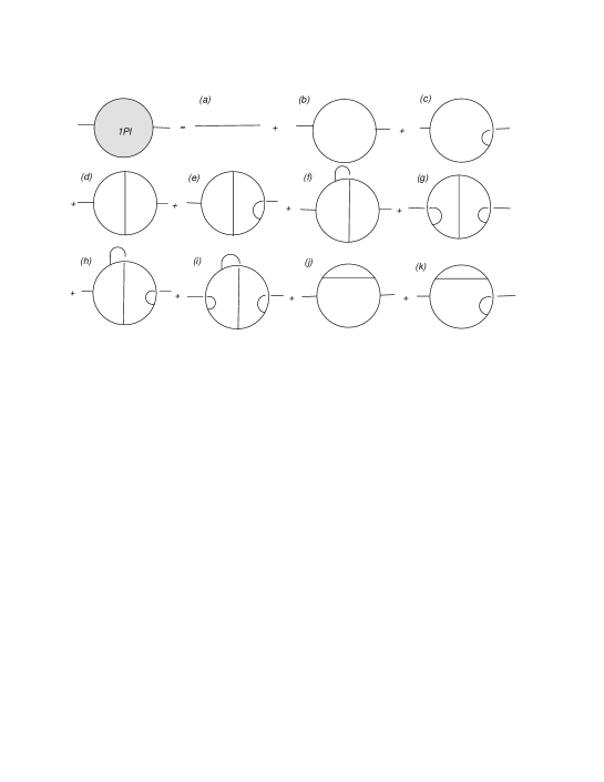
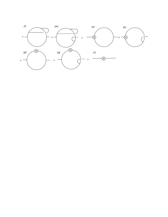
Figure 1: List of diagrams for calculating the two-point function up to the two-loop level.

The diagrams that need to be evaluated in the two-loop calculation of the two-point function are listed in Fig. 1. ( We refer the reader to Ref. rf:MRS for the Feynman rules.) For diagrams (e),(h),(j),(k),(l),(m),(n),(o),(p) and (q), we need to include a factor of 2 to take into account the same contributions from analogous diagrams.

We focus on two types of nonplanar diagrams, diagrams (e) and (f) in Fig. 1. The type 1 diagram is a diagram in which an external line crosses an internal line. This type includes the ultraviolet divergence coming from the planar one-loop subdiagram. We investigate whether this diagram vanishes at infinite external momentum after appropriate renormalization. The type 2 diagram is a diagram in which internal lines cross. Since the non-commutativity parameter $\theta_{\mu\nu}$ does not couple directly to the external momentum in this case, it is not obvious whether the effect of sending the external momentum to infinity is the same as that of sending $\theta_{\mu\nu}$ to infinity. We comment on the remaining non-planar diagrams in §5.

Throughout this paper, we consider the massive case specifically. Technically, this condition simplifies the evaluation of the upper bound on the nonplanar diagrams. Theoretically, this is the more nontrivial case, because in the massless case, the equivalence of the infinite momentum limit and the $\theta\rightarrow\infty$ limit follows from dimensional arguments.

3 Type 1 diagram

Because the type 1 nonplanar diagram includes an ultraviolet divergence, we have to renormalize it by adding a contribution from a diagram involving the one-loop counterterm for the three-point function [ diagram (o) in Fig. 1 ]. After this procedure, we can study the behavior at infinite external momentum. We adopt dimensional regularization and take the space-time dimensionality to be $d=6-\varepsilon$. Because the coupling constant $g$ has dimensions $(\rm{mass})^{(6-d)/2}$, we set $g=\mu^{\frac{\varepsilon}{2}}g_{r}$, where $\mu$ is the renormalization point, and $g_{r}$ is a dimensionless coupling constant. The ultraviolet divergence appears as a $1/\varepsilon$ pole in the $d\rightarrow 6$ limit.

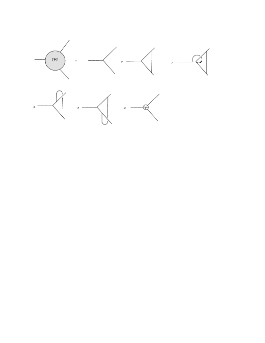
Figure 2: The list of diagrams needed to calculate the three-point function up to the one-loop level.

Figure 3: The planar one-loop diagram for calculating $\Gamma(p,q)$.

The one-loop counterterm for the three-point function can be determined in such a way that the three-point function becomes finite at the one-loop level. The relevant diagrams are listed in Fig. 2. Because the nonplanar diagrams are finite due to the insertion of the momentum dependent phase factor, we only need to calculate the planar diagram depicted in Fig. 3, which can be evaluated as

$$\Gamma(p,q) = g^{3}\int\frac{d^{d}k}{(2\pi)^{d}}\frac{1}{k^{2}+m^{2}}\,\frac{1}{(k-q)^{2}+m^{2}}\,\frac{1}{(k-p)^{2}+m^{2}}$$ (6)

$$= \frac{g^{3}}{(4\pi)^{\frac{d}{2}}}\int_{0}^{1}d\alpha\,\alpha^{\frac{d}{2}-3}(1-\alpha)^{\frac{d}{2}-2}\int_{0}^{1}d\beta\int_{0}^{\infty}dt\,\frac{1}{t^{\frac{d}{2}-2}}\exp(-t\Delta)\ ,$$

where $\Delta$ is defined by

$$\Delta=\frac{m^{2}}{\alpha(1-\alpha)}+q^{2}-2\beta\,p\cdot q+\frac{\beta}{\alpha}\Bigl{(}1-(1-\alpha)\beta\Bigr{)}\,p^{2}\ .$$ (7)

The divergent part can be extracted as

$$\Gamma(p,q)=\frac{g_{r}^{3}}{(4\pi)^{3}}\,\frac{1}{\varepsilon}+\mbox{O}(\varepsilon^{0})\ ,$$ (8)

from which we determine the one-loop counter-term as

$$\delta_{g}=-\frac{g_{r}^{3}}{(4\pi)^{3}}\,\frac{\mu^{\frac{\varepsilon}{2}}}{\varepsilon}\ .$$ (9)

Figure 4: The type 1 nonplanar diagram for calculating $\Pi_{\rm NP1}(p^{2})$.

Using Eq. (6), we evaluate the type 1 nonplanar diagram in Fig. 4 as

$$\Pi_{{\rm NP}1}(p^{2}) = g\int\frac{d^{d}q}{(2\pi)^{d}}\,\Gamma(p,q)\,\frac{1}{q^{2}+m^{2}}\,\frac{1}{(q-p)^{2}+m^{2}}\,e^{iq\cdot\theta p}$$ (10)

$$= \frac{g^{4}}{(4\pi)^{d}}\biggl{[}\frac{4}{(\theta p)^{2}}\biggr{]}^{d-5}\int_{0}^{1}d\alpha\,\alpha^{\frac{d}{2}-3}(1-\alpha)^{\frac{d}{2}-2}\int_{0}^{1}d\beta\int_{0}^{1}d\zeta\,\zeta^{2-\frac{d}{2}}(1-\zeta)$$

$$\cdot\int_{0}^{1}d\eta\int_{0}^{\infty}dt\,t^{d-6}\exp\Bigl{(}-t-\frac{\tilde{\Delta}}{4t}\,p^{2}(\theta p)^{2}\Bigr{)}\ ,$$

where $(\theta p)^{2}\equiv-p^{\mu}\theta^{\mu\nu}\theta^{\nu\rho}p^{\rho}\geq 0$, since $\theta^{\mu\nu}$ is an antisymmetric tensor. The quantity $\tilde{\Delta}$ is defined as

$$\tilde{\Delta}=\frac{m^{2}}{p^{2}}\biggl{[}\frac{\zeta}{\alpha(1-\alpha)}+1-\zeta\biggr{]}+\,\frac{1}{\alpha}\biggl{[}\zeta\,\beta(1-\beta)+\alpha(1-\zeta)\Bigl{(}\zeta(\beta-\eta)^{2}+\eta(1-\eta)\Bigr{)}\biggr{]}\ .$$ (11)

Extracting the divergent part of (10) and taking the $d\rightarrow 6$ limit for the finite part, we obtain

$$\Pi_{{\rm NP}1}(p^{2})=\frac{g_{r}^{4}}{(4\pi)^{6}}\left[\frac{4}{(\theta p)^{2}}\biggl{\{}\frac{\mathcal{A}}{\varepsilon}+\Bigl{(}\ln\,(\pi\mu^{2}(\theta p)^{2})+1\Bigr{)}\,\mathcal{A}-\,\mathcal{B}-\,\mathcal{C}\biggr{\}}+p^{2}\mathcal{D}\right]\ ,$$ (12)

where we have introduced

$$\mathcal{A} = \int_{0}^{1}d\eta\int_{0}^{\infty}dt\,\exp\biggl{[}-t-\frac{\frac{m^{2}}{p^{2}}+\eta(1-\eta)}{4t}\,p^{2}(\theta p)^{2}\biggr{]}\ ,$$ (13)

$$\mathcal{B} = \int_{0}^{1}d\eta\int_{0}^{\infty}dt\,(\ln t)\exp\biggl{[}-t-\frac{\frac{m^{2}}{p^{2}}+\eta(1-\eta)}{4t}\,p^{2}(\theta p)^{2}\biggr{]},\,$$ (14)

$$\mathcal{C} = \int_{0}^{1}d\alpha\int_{0}^{1}d\beta\int_{0}^{1}d\zeta\int_{0}^{1}d\eta\int_{0}^{\infty}dt\,(1-\alpha)\exp\biggl{[}-t-\frac{\tilde{\Delta}}{4t}\,p^{2}(\theta p)^{2}\biggr{]}\ ,$$ (15)

$$\mathcal{D} = \int_{0}^{1}d\alpha\int_{0}^{1}d\beta\int_{0}^{1}d\zeta\int_{0}^{1}d\eta\int_{0}^{\infty}dt\,\frac{F\ln\zeta}{\alpha t}\exp\biggl{[}-t-\frac{\tilde{\Delta}}{4t}\,p^{2}(\theta p)^{2}\biggr{]}\ ,$$ (16)

which are functions of $\frac{m^{2}}{p^{2}}$ and $p^{2}(\theta p)^{2}$. The coefficient $F$ in Eq. (16) is defined by

$$F=\frac{m^{2}}{p^{2}}\Bigl{(}1-\alpha(1-\alpha)\Bigr{)}+(1-\alpha)\biggl{[}\beta(1-\beta)+\alpha\Bigl{(}(1-2\zeta)(\beta-\eta)^{2}-\eta(1-\eta)\Bigr{)}\biggr{]}\ .$$ (17)

We now demonstrate that the functions $\mathcal{A}$, $\mathcal{B}$, $\mathcal{C}$ and $\mathcal{D}$ vanish in the $p^{2}\to\infty$ limit. For this purpose, we first confirm the convergence of all the integrals. Then it will suffice to show that the integrands vanish in the $p^{2}\to\infty$ limit. The convergence of the integrals in $\mathcal{A},\mathcal{B}$ and $\mathcal{C}$ is evident. As for the function $\mathcal{D}$, the $\alpha$- and $t$-integrals would have singularities at the lower ends of the integration domain if $\theta_{\mu\nu}$ were zero, but they are regularized by the term proportional to $1/(\alpha t)$ in the exponent, which appears for nonzero $\theta_{\mu\nu}$. Actually, we can put an upper bound on the absolute values of these functions by integrating elementary functions that are larger than the corresponding integrands. In this way, we obtain upper bounds on $|\mathcal{A}|$, $|\mathcal{B}|$ and $|\mathcal{C}|$ as

$$|\mathcal{A}|<1\ ,\quad|\mathcal{B}|<2\ ,\quad|\mathcal{C}|<1\ ,$$ (18)

by omitting the term proportional to $p^{2}(\theta p)^{2}$ in the exponent. Obtaining an upper bound on $|\mathcal{D}|$ is more involved, due to the “noncommutative” regularization of the singularities mentioned above, but the calculation in Appendix A yields

$$|\mathcal{D}|<\frac{32}{p^{2}(\theta p)^{2}}\Bigl{(}1+\ln\frac{p^{2}}{m^{2}}\Bigr{)}\Bigr{(}4+\ln\frac{p^{2}}{m^{2}}+\ln\frac{p^{2}(\theta p)^{2}}{4}\Bigr{)}\ ,$$ (19)

where we have assumed $m^{2}/p^{2}\ll 1$, since we are ultimately interested in the $p^{2}\rightarrow\infty$ limit. This confirms the convergence. Because the integrands of the functions $\mathcal{A}$, $\mathcal{B}$, $\mathcal{C}$ and $\mathcal{D}$ decrease exponentially at large $p^{2}$, we conclude that all the functions vanish in the $p^{2}\to\infty$ limit.

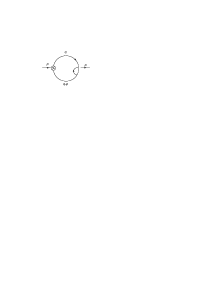
Figure 5: The nonplanar one-loop diagram for calculating $\Pi_{{\rm NP1,ct}}(p^{2})$.

Next we evaluate the diagram in Fig. 5 involving the counterterm (9) as

$$\Pi_{{\rm NP1,ct}}(p^{2}) = \delta_{g}\,g\,\int\frac{d^{d}k}{(2\pi)^{d}}\frac{1}{k^{2}+m^{2}}\,\frac{1}{(k-p)^{2}+m^{2}}\,e^{ik\cdot\,\theta p}$$ (20)

$$= \delta_{g}\,\frac{g}{(4\pi)^{\frac{d}{2}}}\biggl{[}\frac{4}{(\theta p)^{2}}\biggr{]}^{\frac{d}{2}-2}\int_{0}^{1}d\alpha\,\int_{0}^{\infty}dt\,t^{\frac{d}{2}-3}\,\exp\biggl{[}-t-\frac{\frac{m^{2}}{p^{2}}+\alpha(1-\alpha)}{4t}\,p^{2}(\theta p)^{2}\biggr{]}$$

$$= \frac{4g_{r}^{4}}{(4\pi)^{6}}\,\frac{1}{(\theta p)^{2}}\,\left[-\frac{\mathcal{A}}{\varepsilon}+\biggl{\{}-\frac{1}{2}\ln\,(\pi\mu^{2}(\theta p)^{2})\,\mathcal{A}+\,\frac{1}{2}\,\mathcal{B}\biggr{\}}\right]\ .$$

The first term cancels the $1/\varepsilon$ pole in (12), and we have taken the $d\rightarrow 6$ limit for the remaining terms.

Adding (12) and (20), we obtain the finite result

$$\Pi_{{\rm NP1r}}(p^{2})=\frac{g_{r}^{4}}{(4\pi)^{6}}\left[\frac{2}{(\theta p)^{2}}\biggl{\{}\Bigl{(}\ln\,(\pi\mu^{2}(\theta p)^{2})+2\Bigr{)}\mathcal{A}\,-\mathcal{B}-2\,\mathcal{C}\biggr{\}}+p^{2}\mathcal{D}\right]\ .$$ (21)

Because the functions $\mathcal{A}$, $\mathcal{B}$, $\mathcal{C}$ and $\mathcal{D}$ vanish in the $p^{2}\to\infty$ limit, as shown above, the type 1 nonplanar diagram, after renormalizing the divergence from the planar subdiagram, vanishes in the same limit. In fact, using (18) and (19), we obtain an upper bound on $|\Pi_{{\rm NP1r}}(p^{2})|$ as

$$\left|\Pi_{{\rm NP1r}}(p^{2})\right| < \frac{8g_{r}^{4}}{(4\pi)^{6}}\frac{1}{(\theta p)^{2}}$$

$$\cdot\biggl{[}\frac{3}{2}+\frac{1}{4}\ln(\pi\mu^{2}(\theta p)^{2})+4\Bigl{(}1+\ln\frac{p^{2}}{m^{2}}\Bigr{)}\Bigr{(}4+\ln\frac{p^{2}}{m^{2}}+\ln\frac{p^{2}(\theta p)^{2}}{4}\Bigr{)}\biggr{]}\ ,$$

where the right-hand side does vanish in the $p^{2}\rightarrow\infty$ limit, thus confirming the above conclusion more explicitly.

4 Type 2 diagram

In this section, we consider the type 2 nonplanar diagram, in which internal lines cross, and study its behavior in the $p^{2}\to\infty$ limit. Let us first evaluate the one-loop subdiagram in Fig. 6. We have

$$\Gamma_{\rm NP}(p,q) = g^{3}\int\frac{d^{d}k}{(2\pi)^{d}}\frac{1}{k^{2}+m^{2}}\,\frac{1}{(k-q)^{2}+m^{2}}\,\frac{1}{(k-p)^{2}+m^{2}}\,e^{ik\cdot\theta q}$$ (22)

$$= \frac{g^{3}}{(4\pi)^{\frac{d}{2}}}\int_{0}^{1}d\alpha\,\alpha^{\frac{d}{2}-3}(1-\alpha)^{\frac{d}{2}-2}\int_{0}^{1}d\beta\int_{0}^{\infty}dt\,\frac{1}{t^{\frac{d}{2}-2}}$$

$$\cdot\exp\biggl{[}-t\Delta-\frac{\alpha(1-\alpha)}{4t}\,(\theta q)^{2}+i\,\beta\,(1-\alpha)\,p\theta\cdot q\biggr{]}$$

$$= \frac{2g_{r}^{3}}{(4\pi)^{3}}\int_{0}^{1}d\alpha\,(1-\alpha)\int_{0}^{1}d\beta\,e^{i\beta(1-\alpha)p\theta\cdot q}K_{0}\left(\sqrt{\alpha(1-\alpha)\Delta(\theta q)}\right)\$$ (23)

where $K_{0}(z)$ is the modified Bessel function, and $\Delta$ in (22) is defined by

$$\Delta=\frac{m^{2}}{\alpha(1-\alpha)}+q^{2}-2\beta\,p\cdot q+\frac{\beta}{\alpha}\Bigl{(}1-(1-\alpha)\beta\Bigr{)}p^{2}\ .$$ (24)

In proceeding from (22) to (23), we have taken the $d\to 6$ limit. This diagram is finite, as the logarithmic ultraviolet divergence, which would arise in the commutative case, is regularized by the non-commutative phase factor. We can understand this fact by considering the asymptotic behavior of (23)

$$\Gamma_{\rm NP}(p,q)\simeq-\frac{g_{r}^{3}}{2(4\pi)^{3}}\ln p^{2}(\theta q)^{2}$$ (25)

for $(\theta q)^{2}\approx 0$ at nonzero $p^{2}$. This logarithmic behavior reflects the ultraviolet divergence in the commutative case. This can be regarded as a result of the UV/IR mixing.

Figure 6: The nonplanar one-loop diagram for calculating $\Gamma_{\rm NP}(p,q)$.

In what follows, we assume for simplicity that all the eigenvalues of the symmetric matrix $(\theta^{2})^{\mu\rho}=\theta^{\mu\nu}\theta^{\nu\rho}$ are equal, and denote it as $-\theta^{2}\,\,(<0)$. The general case is considered later. In fact, when some of the eigenvalues are zero, there are certain differences in the behavior at large $p^{2}$, but our final conclusion concerning the $p^{2}\rightarrow\infty$ limit is the same.

Figure 7: The type 2 nonplanar diagram for calculating $\Pi_{\rm NP2}(p^{2})$.

Using (22), we evaluate the diagram in Fig. 7 as

$$\Pi_{\rm NP2}(p^{2})$$ (26)

$$= g\int\frac{d^{d}q}{(2\pi)^{d}}\,\Gamma_{\rm NP}(p,q)\frac{1}{q^{2}+m^{2}}\,\frac{1}{(q-p)^{2}+m^{2}}$$

$$= \frac{g^{4}}{(4\pi)^{d}}(p^{2})^{d-5}\int_{0}^{1}d\alpha\,\alpha^{\frac{d}{2}-3}(1-\alpha)^{\frac{d}{2}-2}\int_{0}^{1}d\beta\int_{0}^{1}d\zeta\,\zeta^{2}(1-\zeta)\int_{0}^{1}d\eta$$

$$\cdot\int_{0}^{\infty}dt\,t^{4}\frac{1}{\Bigl{[}t^{2}\zeta+\frac{\alpha(1-\alpha)}{4}\,\theta^{2}(p^{2})^{2}\Bigr{]}^{\frac{d}{2}}}\exp\biggl{[}-t\tilde{\Delta}-t\frac{\tilde{\Delta}_{\rm NP}}{t^{2}\zeta+\frac{\alpha(1-\alpha)}{4}\,\theta^{2}(p^{2})^{2}}\biggr{]}\ ,$$

where we have defined

$$\tilde{\Delta} \equiv \frac{m^{2}}{p^{2}}\biggl{[}\frac{\zeta}{\alpha(1-\alpha)}+1-\zeta\biggr{]}+\frac{\zeta\beta(1-\beta)}{\alpha}+(1-\zeta)\Bigl{(}\zeta(\beta-\eta)^{2}+\eta(1-\eta)\Bigr{)}\ ,\mbox{~{}~{}~{}~{}}$$ (27)

$$\tilde{\Delta}_{\rm NP} \equiv \frac{1-\alpha}{4}\Bigl{[}\zeta\beta^{2}(1-\alpha)+\alpha\bigr{(}\zeta\beta+(1-\zeta)\eta\bigl{)}^{2}\Bigr{]}\theta^{2}(p^{2})^{2}\ .$$ (28)

The $\zeta$- and $t$-integrals would have singularities at the lower ends of the integration domain if $\theta^{2}$ were zero, but they are regularized by the term proportional to $\theta^{2}$ in the denominator. This appearance of the $\theta^{2}$ term is peculiar to nonplanar diagrams in which the internal lines cross [4]. By omitting the $t^{2}\zeta$ term in the denominator and the terms other than those proportional to $m^{2}$ in the exponent, we obtain an upper bound on $|\Pi_{\rm NP2}(p^{2})|$ as

$$|\Pi_{\rm NP\,2}(p^{2})|<\frac{g^{4}}{(4\pi)^{d}}\frac{4^{\frac{d}{2}}}{(\theta^{2})^{\frac{d}{2}}(m^{2})^{5}}\ ,$$ (29)

which confirms the convergence of the multiple integral in (26) in the $d\to 6$ limit. Given this, the fact that the integrand in Eq. (26) decreases as $1/(p^{2})^{5}$ at large $p^{2}$ implies that the type 2 nonplanar diagram vanishes in the $p^{2}\to\infty$ limit. As we have done in the case of type 1 diagrams, we can actually put a more stringent upper bound on $|\Pi_{\rm NP2}(p^{2})|$, indeed, one which vanishes in the $p^{2}\to\infty$ limit. This confirms our assertion more explicitly. (See Appendix B for the details.)

Let us comment on the case in which the number of non-commutative directions is less than the space-time dimensionality, $d$. In this case, the upper bound on $|\Pi_{\rm NP2}(p^{2})|$ can be evaluated as

$$|\Pi_{\rm NP2}(p^{2})| < \frac{g^{4}}{(4\pi)^{d}}(p^{2})^{d-5}\int_{0}^{1}d\alpha\,\alpha^{\frac{d}{2}-3}(1-\alpha)^{\frac{d}{2}-2}\int_{0}^{1}d\beta\int_{0}^{1}d\zeta\,\zeta^{2}(1-\zeta)\int_{0}^{1}d\eta$$ (30)

$$\cdot\int_{0}^{\infty}dt\,t^{4}\prod_{j=1}^{d}\frac{1}{\Bigl{[}t^{2}\zeta+\frac{\alpha(1-\alpha)}{4}\,\theta_{j}^{2}(p^{2})^{2}\Bigr{]}^{\frac{1}{2}}}\exp\Bigl{[}-t\tilde{\Delta}\Bigr{]}\ ,$$

where $(-\theta_{j}^{2})$ is the $j$-th eigenvalue of $(\theta^{2})^{\mu\nu}$, and $\tilde{\Delta}$ is the same as that defined in (27). If non-commutativity is introduced in only $k$ directions $(2\leq k\leq 6)$, we obtain an upper bound from (30), generalizing (29), as

$$|\Pi_{\rm NP2}(p^{2})|<\frac{g^{4}}{(4\pi)^{d}}\frac{a_{k}\cdot 4^{\frac{k}{2}}}{\prod_{j=1}^{k}(\theta_{j}^{2})^{\frac{1}{2}}(m^{2})^{k-1}}\ ,$$ (31)

where $a_{k}$ is a $k$-dependent constant that is irrelevant to the issue with which we are presently concerned. In the $p^{2}\to\infty$ limit, the integrand on the right-hand side of (30) decreases as $(1/p^{2})^{k-1}$. Thus we conclude that the type 2 nonplanar diagram vanishes in the $p^{2}\to\infty$ limit for general $\theta_{\mu\nu}$.

5 Summary and discussion

In this paper we have studied the vanishing of nonplanar diagrams in the $p^{2}\to\infty$ limit in 6d non-commutative $\phi^{3}$ theory at the two-loop level. We have investigated two types of nonplanar diagrams separately. In the type 1 nonplanar diagram, we have confirmed the planer dominance after renormalizing the ultraviolet divergence coming from the planar subdiagram. In the type 2 nonplanar diagram the planer dominance holds despite the fact that the non-commutative phase factor does not depend on the external momentum.

Based on the behavior observed for these two types of diagrams, we can argue that the other types of nonplanar diagrams in Fig. 1 also vanish in the $p^{2}\to\infty$ limit. The situations for the diagrams (k) and (l) are analogous to those for the type 1 and type 2 diagrams, respectively. The diagram (k) has a planar subdiagram, which causes a UV divergence. This divergence can be cancelled by adding the contribution from the diagram (q), and the resulting finite quantity should vanish due to the crossing of an external line and an internal line. The diagram (l) is finite by itself, and it should vanish in a manner similar to the type 2 diagram due to the crossing of internal lines. The diagrams (g),(h) and (i) have more crossings of momentum lines than the type 1 diagram. Therefore for those diagrams, there are extra non-commutative phase factors, which make the diagrams finite by themselves. The vanishing of these diagrams then follows as in the case of the type 1 diagram. An analogous argument applies to the diagram (m), which has more crossings of momentum lines than the diagram (k). Although we have studied a particular model for concreteness, we believe that the same conclusion holds for a more general class of models.

We should mention that the renormalization procedure [18] in non-commutative scalar field theories encounters an obstacle due to severe infrared divergence at higher loops [4]. This problem can be overcome by resumming a class of diagrams with infrared divergence in $\phi^{4}$ theory [4]. Indeed, Monte Carlo simulations show that one can obtain a sensible continuum limit [8], which suggests the appearance of a dynamical infrared cutoff due to nonperturbative effects. Introducing an infrared cutoff with such a dynamical origin in perturbation theory, we believe that the result obtained here up to two-loop order can be generalized to all orders.

Appendix A Derivation of the Upper Bound (19)

In this appendix we derive the upper bound (19) under the condition $\frac{m^{2}}{p^{2}}\ll 1$. Let us consider $\tilde{\Delta}$ and $F$ in Eq. (16). Then, from the relations

$$\tilde{\Delta} = \tilde{\Delta}_{1}+\tilde{\Delta}_{2}\ ,$$

$$\tilde{\Delta}_{1} = \frac{m^{2}}{p^{2}}\biggl{[}\frac{\zeta}{\alpha(1-\alpha)}+1-\zeta\biggr{]}>\frac{m^{2}}{p^{2}}\frac{\zeta}{\alpha}\ ,$$

$$\tilde{\Delta}_{2} = \frac{1}{\alpha}\biggl{[}\zeta\,\beta(1-\beta)+\alpha(1-\zeta)\Bigl{(}\zeta(\beta-\eta)^{2}+\eta(1-\eta)\Bigr{)}\biggr{]}>\frac{\zeta}{\alpha}\beta(1-\beta)\ ,$$

we can put a lower bound on $\tilde{\Delta}$ as

$$\tilde{\Delta}>\frac{\zeta}{\alpha}\Bigl{(}\frac{m^{2}}{p^{2}}+\beta(1-\beta)\Bigr{)}\ . \cdot$$ (A1)

Similarly, we decompose $F$ as $F=F_{1}+F_{2}+F_{3}$, where

$$F_{1} = \frac{m^{2}}{p^{2}}\Bigl{(}1-\alpha(1-\alpha)\Bigr{)}\ ,$$

$$F_{2} = (1-\alpha)\beta(1-\beta)\ ,$$

$$F_{3} = \alpha(1-\alpha)\Bigl{(}(1-2\zeta)(\beta-\eta)^{2}-\eta(1-\eta)\Bigr{)}\ .$$

Then, because $|F_{1}|<1$, $|F_{2}|<1$, $|F_{3}|<2$, we obtain $|F|<4$. Thus we have

$$|\mathcal{D}|<4\int_{0}^{1}\!d\alpha\int_{0}^{1}\!d\beta\int_{0}^{1}\!d\zeta\int_{0}^{1}\!d\eta\,\int_{0}^{\infty}\!dt\,\frac{|\ln\zeta|}{\alpha t}\exp\biggl{[}-t-\frac{\zeta}{4t\alpha}\Bigl{(}\frac{m^{2}}{p^{2}}+\beta(1-\beta)\Bigr{)}p^{2}(\theta p)^{2}\biggr{]}\ .$$

Next we change the integration variable $\zeta$ to $\lambda\equiv\frac{\zeta}{4t\alpha}\Bigl{(}\frac{m^{2}}{p^{2}}+\beta(1-\beta)\Bigr{)}p^{2}(\theta p)^{2}$, and send the upper end of the $\lambda$-integral to $\infty$. This yields

$$|\mathcal{D}| < \frac{16}{p^{2}(\theta p)^{2}}\int_{0}^{1}d\beta\,\frac{1}{\frac{m^{2}}{p^{2}}+\beta(1-\beta)}\,\int_{0}^{1}d\alpha\,\int_{0}^{\infty}dt\int_{0}^{\infty}d\lambda\,e^{-t-\lambda}$$

$$\cdot \biggl{[}\,|\ln t|+|\ln\alpha|+|\ln\lambda|+\left|\ln\Bigr{(}\frac{m^{2}}{p^{2}}+\beta(1-\beta)\Bigl{)}\right|+\left|\ln\frac{p^{2}(\theta p)^{2}}{4}\right|\,\biggr{]}\ .$$

Finally, using the inequalities

$$\left|\,\ln\Bigr{(}\frac{m^{2}}{p^{2}}+\beta(1-\beta)\Bigl{)}\right| < \ln\frac{p^{2}}{m^{2}}\ ,$$

$$\int_{0}^{1}d\beta\,\frac{1}{\frac{m^{2}}{p^{2}}+\beta(1-\beta)} = \frac{1}{\sqrt{\frac{1}{4}+\frac{m^{2}}{p^{2}}}}\ln\frac{\Bigr{(}\sqrt{\frac{1}{4}+\frac{m^{2}}{p^{2}}}+\frac{1}{2}\Bigl{)}^{2}}{\frac{m^{2}}{p^{2}}}<\,2\Bigr{(}1+\ln\frac{p^{2}}{m^{2}}\Bigl{)}\ ,$$

$$\int_{0}^{\infty}dt\,|\ln t|\,e^{-t} \equiv c<\frac{3}{2}\ ,$$

we arrive at the upper bound (19) on $|\mathcal{D}|$.

Appendix B Derivation of a Stringent Upper Bound on $|\Pi_{\rm NP2}(p^{2})|$

In this appendix we obtain an upper bound on $|\Pi_{\rm NP2}(p^{2})|$ that is more stringent than Eq. (29) and actually vanishes in the $p^{2}\rightarrow\infty$ limit. Let us consider the integrand in the last line of (26). In the denominator we omit the $t^{2}\zeta$ term, and in the exponent we omit $\tilde{\Delta}_{\rm NP}$ and the term $(1-\zeta)\Bigl{(}\zeta(\beta-\eta)^{2}+\eta(1-\eta)\Bigr{)}$ in $\tilde{\Delta}$. Thus, we obtain the upper bound

$$|\Pi_{\rm NP2}(p^{2})|<\frac{g^{4}}{(4\pi)^{d}}\Bigr{(}\frac{4}{\theta^{2}}\Bigl{)}^{\frac{d}{2}}\frac{1}{(m^{2})^{5}}\,G\Bigr{(}\frac{m^{2}}{p^{2}}\Bigl{)}\ , \cdot$$ (B1)

where the function $G(x)$ is defined by

$$G(x) = x^{5}\int_{0}^{1}\,d\beta\int_{0}^{1}\,d\alpha\int_{0}^{1}\,d\zeta\,\frac{24\,\alpha^{2}(1-\alpha)^{3}\zeta^{2}(1-\zeta)}{\Bigl{[}x\bigl{(}\zeta+\alpha(1-\alpha)(1-\zeta)\bigr{)}+\zeta(1-\alpha)\beta(1-\beta)\Bigr{]}^{5}} \cdot$$ (B2)

$$= \frac{\frac{1}{2}x^{2}}{\Bigr{(}\frac{1}{4}+x\Bigl{)}^{\frac{3}{2}}}\Biggl{(}\ln\frac{\sqrt{\frac{1}{4}+x}+\frac{1}{2}}{\sqrt{\frac{1}{4}+x}-\frac{1}{2}}+\frac{1}{x}\sqrt{\frac{1}{4}+x}\Biggr{)}\ .$$

Then, because $\lim_{x\rightarrow 0}G(x)=0$, Eq. (B$\cdot$1) confirms explicitly that $\Pi_{\rm NP2}(p^{2})$ vanishes in the $p^{2}\to\infty$ limit.

References

[1] H. S. Snyder,
Phys. Rev. 71 (1947), 38.
A. Connes,