The Conformal Limit of the 0A Matrix Model and String Theory on AdS₂

Abstract:

We analyze the conformal limit of the matrix model describing flux backgrounds of two dimensional type 0A string theory. This limit is believed to be dual to an AdS₂ background of type 0A string theory. We show that the spectrum of this limit is identical to that of a free fermion on AdS₂, suggesting that there are no closed string excitations in this background.

1 Introduction and Summary

Two dimensional non-critical string theories are useful toy models for studying various aspects of string theory (for reviews see [1, 2, 3]). In particular, the two dimensional type 0 string theories are useful for this, since they are non-perturbatively stable and they have a known matrix model dual [4, 5]. Since the type 0 theories have Ramond-Ramond (RR) fields, they can be used to study RR backgrounds, whose worldsheet description in string theory is still poorly understood.

The type 0A theory has RR 2-form field strengths which are sourced by D0-branes. It has been suggested that this theory should have an AdS₂ solution with RR flux. This is based both on the fact that the space-time effective action has an extremal black hole solution whose near-horizon limit is AdS₂, and on the fact that the matrix model for the 0A theory with flux has a limit in which it is a conformally invariant quantum mechanical system (which one expects to be dual via the AdS/CFT correspondence to an AdS₂ background of string theory) [6, 7]. If such a background exists, it is interesting to study it, both as a simple example of a RR background (the large symmetry may help in finding a useful worldsheet description of this background) and as an example of the correspondence between AdS₂ backgrounds and conformal quantum mechanics, which is still not as well understood as other examples of the AdS/CFT correspondence.

In this note we study the conformal limit of the 0A matrix model in order to find the properties of this conjectured AdS₂ background. We find that the spectrum of this theory is equal to that of a free fermion field on AdS₂, with a mass proportional to the RR flux $q$. This fermion originates from the eigenvalues of the matrix model which correspond to D0-anti-D0-brane pairs, so this spectrum suggests that the only excitations in this AdS₂ background are such uncharged D-brane-pairs, and that there are no closed string excitations in this background. From the point of view of 0A backgrounds with flux which asymptote to a linear dilaton region, this implies that the closed string excitations cannot penetrate into the strongly coupled region which is dual to the conformal limit of the matrix model.

We begin in section 2 by reviewing two dimensional type 0A string theory, its matrix model description, and its extremal black hole background. In section 3 we analyze the conformal limit of the matrix model and compute its spectrum. In section 4 we discuss the implications of this spectrum for the dual string theory on AdS₂, and in section 5 we discuss bosonizations of the fermionic system we find, which may be useful for studying the conformal quantum mechanics with a non-zero Fermi level. In the appendix we provide a detailed computation of the spectrum of a spinor field on AdS₂.

2 A Brief Review of Type 0A Superstrings

2.1 Type 0A Spacetime Effective Action

Two dimensional fermionic strings are described by $\mathcal{N}=1$ supersymmetric worldsheet field theories coupled to worldsheet supergravity. The non chiral GSO projection gives the two type 0 theories. Because there are no NS-R or R-NS sectors in the theory, the type 0 theories have no fermions and are not supersymmetric in spacetime. The NS-NS sector includes a graviton, a dilaton and a tachyon. In two dimensions, there are no transverse string oscillations, and longitudinal oscillations are unphysical except at special values of the momentum. Thus, the tachyon is the only physical NS-NS sector field. In type 0A, the R-R sector contributes two 1-forms, and the action is [4] (with $\alpha^{\prime}=2$)

$$S=\int d^{2}x\sqrt{-g}\bigg{[}\frac{e^{-2\Phi}}{2\kappa^{2}}\bigg{(}4+R+4(\nabla\Phi)^{2}-\frac{1}{2}(\nabla T)^{2}+\frac{1}{2}T^{2}+\dotsb\bigg{)}-\\ -\pi e^{-2T}(F^{(+)})^{2}-\pi e^{2T}(F^{(-)})^{2}+\dotsb\bigg{]}.$$ (1)

The equations of motion are solved by a linear dilaton solution

$$G_{\mu\nu}=\eta_{\mu\nu}, \Phi=x,$$ (2)

where $x$ is the spatial coordinate. A possible deformation is to turn on the tachyon (whose mass is lifted to zero by the linear dilaton) $T=\mu e^{x}$.

The general equations of motion are

$$\begin{split}0&=2R_{\mu\nu}+4\nabla_{\mu}\nabla_{\nu}\Phi-\nabla_{\mu}T\nabla_{\nu}T+2\pi\kappa^{2}e^{2\Phi-2T}[g_{\mu\nu}(F^{(+)})^{2}-4(F^{(+)})_{\mu}^{\beta}(F^{(+)})_{\nu\beta}]+\\ &+2\pi\kappa^{2}e^{2\Phi+2T}[g_{\mu\nu}(F^{(-)})^{2}-4(F^{(-)})_{\mu}^{\beta}(F^{(-)})_{\nu\beta}],\end{split}$$ (3a)

$$0 =-2-\nabla^{2}\Phi+2(\nabla\Phi)^{2}-\frac{1}{4}T^{2}-\pi\kappa^{2}e^{2\Phi}[e^{-2T}(F^{(+)})^{2}+e^{2T}(F^{(-)})^{2}],$$ (3b)

$$0 =\nabla^{2}T-2\nabla\Phi\cdot\nabla T+T+4\pi\kappa^{2}e^{2\Phi}[e^{-2T}(F^{(+)})^{2}-e^{2T}(F^{(-)})^{2}],$$ (3c)

$$0 =\nabla^{\nu}(e^{\mp 2T}F^{(\pm)}_{\mu\nu}).$$ (3d)

Equation (3d) implies

$$0=\nabla_{\nu}(e^{\mp 2T}F^{(\pm)\mu\nu})=\partial_{\nu}(\sqrt{-g}e^{\mp 2T}F^{(\pm)\mu\nu})=\begin{cases}-\partial_{0}(\sqrt{-g}e^{\mp 2T}F^{(\pm)01})\\ \partial_{1}(\sqrt{-g}e^{\mp 2T}F^{(\pm)01})\end{cases},$$ (4)

i.e. $\sqrt{-g}e^{\mp 2T}F^{(\pm)01}$ is constant. Thus, we see that the zero modes are the only degrees of freedom of the vector field. Furthermore, due to the non trivial coupling in front of $(F^{\pm})^{2}$, a time independent field strength can only be turned on for the vector field whose coupling $e^{\pm 2T}$ does not vanish at infinity. For example, in the linear dilaton background, the solutions of (4) are

$$F^{(+)}_{01} =q^{+}e^{+2T}, F^{(-)}_{01} =q^{-}e^{-2T}.$$ (5)

Suppose that $\mu<0$. As $x\rightarrow\infty$, $T\rightarrow-\infty$ and $F^{(-)}$ becomes singular, while $F^{(+)}$ is regular. Thus, turning on $F^{(-)}$ requires having D-branes as a source for this field, while no such branes are needed for $F^{(+)}$. These D-branes carry RR 1-form charge, so these are D0-branes (known as ZZ-branes). For positive $\mu$ the situation is reversed. Thus, both $q^{+}$ and $q^{-}$ are quantized. For $\mu=0$ it seems that we can turn on both fields, however, as shown in [8], this requires the insertion of $q^{+}q^{-}$ strings that stretch from $x=-\infty$ to the strongly coupled region. This leads to additional terms in the effective action (1) (see also [9]).

2.2 Matrix Model Description

In analogy to the bosonic case [10], it was conjectured in [4, 5] that the field theory on $N$ such D0-branes (with $N\rightarrow\infty$) is a dual description of the full string theory. It was argued there that the matrix model that gives the linear dilaton background of the 0A theory is a U$(N)_{A}\times$U$(N)_{B}$ gauge theory with a complex matrix $m$ in the bifundamental representation. The two $U(N)$ groups originate from D0 and anti-D0 branes.

There are two ways of introducing RR flux [4]. First, we can modify the gauge group to U$(N)_{A}\times$U$(N+q^{-})_{B}$. This leads to $q^{-}\neq 0$, $q^{+}=0$ and corresponds to placing $N+q^{-}$ ZZ-branes and $N$ anti-ZZ-branes at $x=+\infty$. As long as the Fermi level is below the barrier ($\mu<0$), we will have $q^{-}$ charged ZZ-branes left over after the open string tachyon condenses, so this is expected to correspond to the background with $q^{-}$ units of $F^{(-)}$ flux and no $F^{(+)}$ flux. When reducing this rectangular matrix model to fermionic eigenvalue dynamics one finds that the potential for the eigenvalues is [11]

$$V(\lambda)=-\frac{1}{8}\lambda^{2}+\frac{M}{2\lambda^{2}},$$ (6)

where $M=(q^{-})^{2}-1/4$ and $\lambda$ stands for the positive square roots of the eigenvalues of $m^{\dagger}m$. $\lambda$ should be thought of as a radial coordinate, i.e. $\lambda\in[0,\infty)$.

A second way to introduce flux, for $q^{+}\neq 0$, $q^{-}=0$, is to add a term of the form

$$S=S_{0}+iq^{+}\int(\operatorname{Tr}A-\operatorname{Tr}B)dt,$$ (7)

where $A$ and $B$ are the gauge fields of the U($N)_{A}$ and U$(N)_{B}$ gauge groups respectively. This has the effect of constraining the eigenvalues of $m$ to move in a plane, all with angular momentum $q^{+}$. Surprisingly, the reduction to eigenvalues of $m^{\dagger}m$ gives exactly the potential (6) with $M=(q^{+})^{2}-1/4$.

We may try to turn on both $q^{+}$ and $q^{-}$ at the same time. It was shown in [8] that this leads again to the same potential with $M=(|q^{+}|+|q^{-}|)^{2}-1/4$. Thus, we see that from the point of view of the matrix model, the theory depends on $|q|\equiv|q^{+}|+|q^{-}|$ alone. Due to this and supported by arguments from the target space theory, it was argued in [8] that physics depends only on $|q|$. This point will be important in the next subsection where we discuss the two dimensional black hole solution, which requires turning on both fluxes.

2.3 The Extremal Black Hole Solution

The equations of motion (3a)-(3d) also admit a solution that is often referred to as the 2d extremal black hole solution [6, 12, 13]

$$ds^{2} =\left[1+\frac{q^{2}}{8}\left(\Phi-\Phi_{0}-\frac{1}{2}\right)e^{2\Phi}\right](-dt^{2}+dx^{2}),$$ (8a)

$$F^{(+)} =F^{(-)}=\frac{q}{2}dt\wedge dx,$$ (8b)

$$T =0,$$ (8c)

where $\Phi_{0}=-\log\frac{q}{4}$ and $\Phi$ is given implicitly by the ODE

$$\frac{1}{2}\frac{d\Phi}{dx}=1+\frac{q^{2}}{8}\left(\Phi-\Phi_{0}-\frac{1}{2}\right)e^{2\Phi}.$$ (9)

The boundary conditions are set such that at the asymptotic region $x\rightarrow-\infty$ the solution approaches the linear dilaton solution. In the $x\rightarrow+\infty$ region the solution becomes AdS₂ with string coupling $g_{s}=4/q$ :

$$ds^{2} \rightarrow\frac{1}{8x^{2}}(-dt^{2}+dx^{2}), F^{(+)} =F^{(-)}=\frac{q}{2}dt\wedge dx, \Phi \rightarrow\Phi_{0}.$$ (10)

There are two major problems with this solution. The first is that the curvature becomes large as $x\rightarrow+\infty$, specifically, at the AdS₂ region of this solution $R=-8$ (in string units), so higher order corrections to (1) are important and the solution is invalid there. Note that unlike the linear dilaton background, this solution is not an exact CFT. The second problem is that this solution requires turning on both of the 0A vector fields, which, as we mentioned before, implies that one needs to add strings to the background and take their effects into account. Furthermore, the study of the background $(q^{+},q^{-})=(q^{+},0)$ shows that there is no entropy and no classical absorption. Thus, if the physics indeed depends only on $|q|$, then a black hole is not expected to exist.

It was suggested in [7] that perhaps, despite these problems, a solution that interpolates between a linear dilaton region and an AdS₂ region exists for the full theory. If this is the case, then by the AdS/CFT correspondence [14], the AdS₂ region of the solution would be dual to a one dimensional CFT (or conformal quantum mechanics (CQM)), and it was conjectured in [7] that this CQM is the conformal limit of the 0A matrix model. In the next sections we will analyze this CQM to see what the properties of such a solution must be.

3 The Conformal Limit of the Matrix Model

The 0A matrix model eigenvalues move in the potential (see Figure 1)

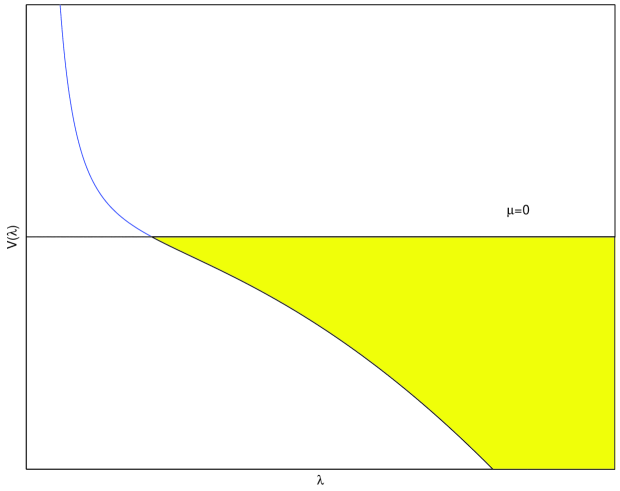
Figure 1: The potential for the eigenvalues of the matrix model describing 0A string theory in a background with non-zero flux, with Fermi level $\mu=0$.

$$V(\lambda)=-\frac{1}{8}\lambda^{2}+\frac{M}{2\lambda^{2}}\;.$$ (11)

At large $\lambda$ the second term is negligible and the dynamics are as in the original $q=0$ linear dilaton background. At small $\lambda$ one can ignore the $\lambda^{2}$ term and remain with the action

$$S=\frac{1}{2}\int dt\left(\dot{\lambda}^{2}-\frac{M}{\lambda^{2}}\right).$$ (12)

This action was studied in detail in [15] as the simplest example of a (nontrivial) conformal field theory in one dimensional space (only time). It is invariant under the SL(2,$\mathbb{R}$) group of transformations given by

$$t\rightarrow t^{\prime}=\frac{at+b}{ct+d}, \lambda(t)\rightarrow\lambda^{\prime}(t^{\prime})=(ct+d)^{-1}\lambda(t),$$ (13)

with $ad-bc=1$. The generators of these transformations are

$$H =\frac{1}{2}\dot{\lambda}^{2}+\frac{M}{2\lambda^{2}}, K =\frac{1}{2}\lambda^{2}, D =-\frac{1}{4}(\lambda\dot{\lambda}+\dot{\lambda}\lambda).$$ (14)

Note that the AdS/CFT correspondence maps $H$ to time evolution in the Poincaré time coordinate of AdS₂. It is important to emphasize that the AdS₂ vacuum is supposed to be mapped to the solution with $\mu=0$, since a finite Fermi sea would break conformal invariance. The relation to SO(2,1) is made evident by taking the linear combinations

$$L_{01} =S=\frac{1}{2}\left(\frac{1}{r}K-rH\right), L_{02} =D, L_{12} =R=\frac{1}{2}\left(\frac{1}{r}K+rH\right).$$ (15)

(for any constant $r$). Here $L_{\mu\nu}$ are rotations in the $\mu\nu$ plane, thus, the operator $R$ is compact. It should also be noticed that the three operators are related by a constraint in this system

$$\frac{1}{2}(HK+KH)-D^{2}=\frac{M}{4}-\frac{3}{16}=\frac{q^{2}-1}{4}$$ (16)

(this is why one seems to have three constants of motion in a two dimensional phase space).

The essential observation of [15] is that by a reparametrization of time and field,

$$d\tau =\frac{dt}{u+vt+wt^{2}}, \tilde{\lambda}(\tau) =\frac{\lambda(t)}{\sqrt{u+vt+wt^{2}}},$$ (17)

one may transform the action to a different action where the new corresponding Hamiltonian ($\tau$-translation operator) is $G=uH+vD+wK$. Specifically, by choosing $(u,v,w)=(r,0,r^{-1})$ one gets the transformation

$$\tilde{\lambda}(\tau) =\frac{\sqrt{r}}{\sqrt{r^{2}+t^{2}}}\lambda(t), \tau =\arctan(t/r).$$ (18)

The transformed action is

$$S=\frac{1}{2}\int d\tau\left[(\partial_{\tau}\tilde{\lambda})^{2}-\tilde{\lambda}^{2}-\frac{M}{\tilde{\lambda}^{2}}\right],$$ (19)

whose Hamiltonian is the compact operator $R$. The spectrum of $R$ is found using standard algebraic methods to be [15]

$$r_{n} =r_{0}+n, r_{0} =\frac{1}{2}(1+\sqrt{M+1/4})=\frac{1+|q|}{2}\,.$$ (20)

The relations of the $R$ eigenstates to the $H$ eigenstates is also given in [15], as well as general methods of computing transition matrix elements exactly. Obviously, the spectrum of $H$ is continuous and $D$-transformations rescale the eigenvalues of $H$.

As usual in the AdS/CFT correspondence, time evolution by $R$ is supposed to be dual to time evolution of 0A string theory on AdS₂ in global coordinates [7]. The SL(2,$\mathbb{R}$) generators in the language of the new time parameter generate the transformations

$$D \delta\tau =2\sin\tau \delta\lambda =\lambda$$ (21a)

$$H \delta\tau =\frac{1}{r}(1+\cos\tau) \delta\lambda =0$$ (21b)

$$K \delta\tau =r(1-\cos\tau) \delta\lambda =-r\tan(\tau/2)\lambda$$ (21c)

Indeed, this corresponds to the generators of the AdS₂ isometries near the boundary (33). A more complete analysis of the relation between the isometries and different parametrizations of AdS₂ is given in [16].

The original matrix model gives $N$ non-interacting fermions moving in the full potential (6). After taking the CQM limit, we expect some number of these fermions to “live” in the small $\lambda$ region, leading in the large $N$ limit to a second quantized version of (12). Note that the gauge-invariant operators in the matrix model are given by

$$\Lambda_{n}=\operatorname{Tr}\left[(m^{\dagger}m)^{n}\right]=\sum_{i=1}^{N}\lambda_{i}^{2n}$$ (22)

and in the CQM their mass dimension is $(-n)$ (recall that $\lambda_{i}$ are the positive roots of the eigenvalues of $m^{\dagger}m$).

4 The AdS₂ Dual of the CQM

We have seen that the spectrum of the operator $R$ in the CQM is $r_{n}=r_{0}+n$ (see (20)). Thus, since the eigenvalues are fermionic, the spectrum of $R$ in the second quantized CQM is given by stating for each level, $r_{n}$, whether it is occupied or vacant. We would like to identify this with the spectrum of some global AdS₂ solution of type 0A string theory, which would be a corrected version of (10). In fact, this is precisely the same as as the spectrum of a single free fermion field on AdS₂. Recall (as we review in the appendix) that the spectrum of a spinor field of mass $m$ in global AdS₂ (with radius of curvature $r$) is

$$E_{n}=\frac{1}{2}+|mr|+n.$$ (23)

The spectra match if we take a spinor on AdS₂ with mass $mr=|q|/2$. We suggest (based on the origin of the eigenvalues) that the excitations of this spinor field are brane-anti-brane pairs. Since these states account for the full spectrum of the CQM, we suggest that all other fields (in particular the tachyon) have no physical excitations in AdS₂. We have reached this conclusion by analyzing the spectrum in global coordinates, but of course it should apply to the Poincaré coordinates of AdS₂ as well.

We expect that the matrix model with the original potential (6) and with Fermi level $\mu=0$ should correspond to a flux background of 0A which interpolates between a weakly coupled linear dilaton region and a Poincaré patch of AdS₂ (as in the extremal black hole solutions of section 2.3). We can check if the absence of the tachyon field in the AdS₂ region is consistent with this expectation. In the linear dilaton region, tachyon excitations are mapped to excitations of the surface of the Fermi sea in the matrix model. Before taking the “near horizon” limit the classical trajectory of a fermion moving in the potential (6) with energy $E=(\alpha^{\prime})^{-1/2}\varepsilon$ has a turning point at

$$\lambda_{\text{max}}=(\alpha^{\prime})^{1/4}\sqrt{\sqrt{2M+\varepsilon^{2}}-\varepsilon}$$ (24)

(where we have reinstalled $\alpha^{\prime}$). Since the quadratic term in (6) has a coefficient $1/(4\alpha^{\prime})$, the conformal limit is achieved by taking $\alpha^{\prime}\rightarrow\infty$. We wish to consider what happens to a state in the matrix model (6) corresponding to a tachyon excitation (with a finite energy in string units) when we take this limit, so we keep $\varepsilon$ fixed. Clearly, the limit drives the turning point to infinity. Namely, a finite excitation of the surface of the Fermi sea in the asymptotic region of the original matrix model does not penetrate into the region that we are interested in. On the other hand, fermions with very high excitation energies can penetrate into the CQM region, and we identify them with the fermionic excitations on AdS₂ discussed above.

This result suggests that the string dual of this AdS₂ background, expected to be a strongly coupled theory on the worldsheet, has the property that all closed string states in the theory are non-physical (except for, perhaps, discrete states at special momenta). We also predict that the brane-anti-brane excitations of this theory have masses proportional to the RR flux. This suggests that perhaps the string coupling of the dual is $g_{s}\sim 1/q$ as in (10) [6, 7], but it is not clear how to define the string coupling in the absence of string states.

Naively one may have expected that the theory on AdS₂ should contain bosonic fields which are dual to the gauge-invariant operators (22) of the matrix model, as usual in the AdS/CFT correspondence. At first sight this seems to be inconsistent with the fact that we find no bosonic fields in the bulk. Presumably, the operators (22) are mapped to complicated combinations of the fermion field we found.

One of the general mysteries associated with AdS₂ backgrounds in string theory is the fact that they can fragment into multiple copies of AdS₂ (related to the possibility for extremal black holes to split) [17]. Here we find no sign of this phenomenon. Presumably this is related to the fact that there are no transverse directions for the D-branes to be separated in.

5 Remarks on Bosonization

Even though we found that the spectrum of the CQM can be identified with that of a free fermion field on AdS₂, it is interesting to ask if there could also be an alternative bosonic description of the same theory, which could perhaps be interpreted as a closed string dual description. The context in which it seems most likely that such a description would exist is when we look at the CQM (12) with time evolution by $H$, and turn on a finite positive Fermi level $\mu$. This will clearly break the SL(2,$\mathbb{R}$) conformal symmetry (and hence the spacetime isometry on the string side), so it should no longer be dual to an AdS₂ background (note that such a state has infinite energy, so perhaps the corresponding background is not even asymptotically AdS₂). In such a configuration there are excitations of the surface of the Fermi sea with arbitrarily low energies, and these could perhaps be mapped to the tachyon field, as was the case in (6) before taking the “near horizon” limit. Thus, it is interesting to search for a possible alternative description of this state (except for filling the Fermi sea of the brane-anti-brane excitations).

A method that has proven to be very fruitful for studying the matrix model in the past is that of the “collective field formalism”. This method of bosonization, achieved by studying the dynamics of the Fermi liquid in phase space, has led to the computation of scattering amplitudes and other important quantities in the matrix model (e.g. [3, 18, 19]). However, there is an important difference between the CQM and the standard linear dilaton matrix model: in the CQM for momentum $p$ and $t\rightarrow\pm\infty$ we have $\lambda\sim p\,t$, while in the linear dilaton case we have $p\sim\mp\lambda$. Suppose that at some finite time we construct a small pulse perturbing the shape of the Fermi sea. The relation $\lambda\sim p\,t$ means that after (and before) a finite amount of time the pulse will “break up”, or more explicitly, the pulse will no longer admit a description in terms of the upper and lower surfaces of the Fermi liquid. We can follow through the steps of the collective field formalism in order to analyze propagation of pulses along short time intervals or calculate some other quantities, but the elementary excitations of the bosonized version will not be asymptotic states.

This asymptotic behavior of the classical solutions is, of course, a consequence of the fact that the potential is constant as $\lambda\rightarrow+\infty$. One may thus seek other methods of bosonization that are suitable for systems with this property. However, the resulting bosonic systems always seem to have non-local interactions (for instance, this happens in the method presented in [20]). We have not been able to find a bosonic theory with local interactions, which could be interpreted as a bosonic field on some spacetime dual to the CQM with finite $\mu$. It would be interesting to investigate this further.

Appendix A Spinor Fields on AdS₂

A.1 Definitions of AdS₂

The metric on AdS₂ may be written in so called global coordinates as

$$ds^{2}=\frac{r^{2}}{\cos^{2}\theta}(-d\tau^{2}+d\theta^{2}),$$ (25)

where $\tau\in\mathbb{R}$, $\theta\in[-\pi/2,\pi/2]$, and $r$ is the AdS radius of curvature. This is (conformally) an infinite strip, the boundaries at $\theta=\pm\pi/2$ being each a line. Another set of coordinates is the Poincaré coordinates ($t\in\mathbb{R}$ and $x\in\mathbb{R}^{+}$), where the line element is given by

$$ds^{2}=\frac{r^{2}}{x^{2}}(-dt^{2}+dx^{2}).$$ (26)

The relation between the coordinate sets is

$$x=\frac{r\cos\theta}{\cos\tau-\sin\theta}, t=\frac{r\sin\tau}{\cos\tau-\sin\theta},$$ (27)

or

$$\tan\tau=\frac{2rt}{x^{2}-t^{2}+r^{2}}, \tan\theta=\frac{t^{2}-x^{2}+r^{2}}{2rx}.$$ (28)

The generators of isometries in the Poincaré coordinates are

$$H=i\partial_{t}, D=i(t\partial_{t}+x\partial_{x}), K=i((t^{2}+x^{2})\partial_{t}+2tx\partial_{x}),$$ (29)

and in global coordinates

$$rH =i[(1-\cos\tau\sin\theta)\partial_{\tau}+\sin\tau\cos\theta\partial_{\theta}],$$ (30)

$$K/r =i[(1+\cos\tau\sin\theta)\partial_{\tau}-\sin\tau\cos\theta\partial_{\theta}],$$ (31)

$$D =i[-\sin\tau\sin\theta\partial_{\tau}+\cos\tau\cos\theta\partial_{\theta}].$$ (32)

Near the boundaries these become

$$rH =i(1\mp\cos\tau)\partial_{\tau}, K/r =i(1\pm\cos\tau)\partial_{\tau}, D =\mp i\sin\tau\partial_{\tau}.$$ (33)

A.2 Quantization of Spinor Fields on AdS₂ in Global Coordinates

Consider a spinor field on AdS₂ (in global coordinates). In this section we work with signature $(+,-)$. The vierbein is

$$V^{a}_{\mu}=\frac{r}{\cos\theta}\delta^{a}_{\mu}$$ (34)

($\mu$ is a tensor index and $a$ is an index in the local inertial frame). The spin connection is

$$\Gamma_{\mu}=\frac{1}{2}\Sigma^{ab}V_{a}^{\nu}\nabla_{\mu}V_{b\nu}=\delta_{\mu}^{0}\tan\theta\Sigma^{01},$$ (35)

where

$$\Sigma^{01}=\begin{pmatrix}1/2&0\\ 0&-1/2\end{pmatrix}.$$ (36)

The $\gamma$ matrices are chosen to be

$$\gamma^{0}=(r^{-1}\cos\theta)\sigma^{1}, \gamma^{1}=(r^{-1}\cos\theta)i\sigma^{2},$$ (37)

so that the Dirac equation, $(i\gamma^{\mu}\nabla_{\mu}-m)\psi=0$, may be written as

$$\begin{pmatrix}imr\sec\theta&\partial_{0}-\partial_{1}-\frac{1}{2}\tan\theta\\ \partial_{0}+\partial_{1}+\frac{1}{2}\tan\theta&imr\sec\theta\end{pmatrix}\psi=0.$$ (38)

Let $\psi(\theta,\tau)=e^{-i\omega\tau}\cos^{1/2}\theta(e^{i\omega\theta}u(\theta),e^{-i\omega\theta}v(\theta))$. Equation (38) becomes

$$\frac{d}{d\theta}\begin{pmatrix}u\\ v\end{pmatrix}=imr\sec\theta\begin{pmatrix}0&-e^{-2i\omega\theta}\\ e^{2i\omega\theta}&0\end{pmatrix}\begin{pmatrix}u\\ v\end{pmatrix}.$$ (39)

This yields the second order equation

$$\cos^{2}\theta u^{\prime\prime}+\cos\theta(2i\omega\cos\theta-\sin\theta)u^{\prime}-(mr)^{2}u=0.$$ (40)

Substituting $z=(1+i\tan\theta)/2$, we have the hypergeometric equation

$$z(1-z)u^{\prime\prime}+(\frac{1}{2}+\omega-z)u^{\prime}+(mr)^{2}u=0.$$ (41)

The Dirac norm is

$$(\psi_{\omega},\psi_{\omega^{\prime}})=\int_{-\pi/2}^{\pi/2}d\theta\sqrt{-g}\,\psi_{\omega}^{\dagger}\psi_{\omega^{\prime}}=r^{2}\int_{-\pi/2}^{\pi/2}\frac{d\theta}{\cos\theta}(u^{*}u+v^{*}v),$$ (42)

so we shall require the solutions of (41) to vanish at the boundaries ($z\rightarrow\infty$). We will show that this requirement implies that

$$|\omega|=|mr|+\frac{1}{2}+n,\qquad n=0,1,2,\cdots$$ (43)

Equation (41) has three (regular) singular points $\{0,1,\infty\}$. The pairs of exponents at each point are, respectively,

$$\{(0,1/2-\omega),(0,1/2+\omega),(mr,-mr)\}.$$ (44)

When the difference between two exponents at a given point is not an integer the equation has two power-law solutions at that point (when this happens we shall call this point “normal”). When the difference is an integer there is one power-law and one log solution (when this happens we shall call the relevant point “special”). Thus, we see that the proposed result (43) implies that we have three distinct cases: (i) $2mr\not\in\mathbb{Z}$, in which case all three points are normal; (ii) $mr\in\mathbb{Z}$, in which case all points are special; and (iii) $mr+1/2\in\mathbb{Z}$, in which case $z=\infty$ is special and $z=0,1$ are normal.

(i) $2mr\not\in\mathbb{Z}$

In this case there are two power-law solutions at $z=\infty$. According to the sign of $m$, one of the solutions diverges at the boundary and the other one is

$$u_{1}(z)=z^{-|mr|}F(|mr|,|mr|+\frac{1}{2}-\omega,2|mr|+1;z^{-1}).$$ (45)

As $\theta$ goes from $-\pi/2$ to $\pi/2$, the path drawn by $z^{-1}(\theta)$ is a unit circle around $z^{-1}=1$. Along this circle the hypergeometric function has a pole at $z^{-1}=0$ (which we have taken care of), but may also has a branch cut along $z^{-1}\in[1,\infty)$. We must make sure that the solution (45) is continuous (single valued) along the circle. One option is to take $|mr|+1/2-\omega=-n$ ($n\in\mathbb{N}$), so that the power expansion of the hypergeometric function in (45) terminates after a finite amount of terms and the function degenerates into a polynomial. In this case we can choose the branch-cut to be $(-\infty,0]$, which makes $z^{-|mr|}$ single valued, and so (45) is single valued.

When $|mr|+1/2-\omega$ is not a non-positive integer the hypergeometric function will have a branch cut at $[1,\infty)$ and we must try to cancel this discontinuity with the discontinuity in $z^{-|mr|}$. For $\omega+1/2\not\in\mathbb{Z}$, the solution at $z=\infty$ is related to the solutions at $z=1$ through the identity

$$F(|mr|,|mr|+\frac{1}{2}-\omega,2|mr|+1;z^{-1})=\\ =\frac{\Gamma(1+2|mr|)\Gamma(1/2+\omega)}{\Gamma(1+|mr|)\Gamma(1/2+|mr|+\omega)}F(|mr|,|mr|+\frac{1}{2}-\omega,\frac{1}{2}-\omega;1-z^{-1})+\\ +\frac{\Gamma(1+2|mr|)\Gamma(-\frac{1}{2}-\omega)}{\Gamma(|mr|)\Gamma(|mr|+\frac{1}{2}-\omega)}(1-z^{-1})^{1/2+\omega}F(1+|mr|,|mr|+\frac{1}{2}+\omega,\frac{3}{2}+\omega;1-z^{-1}).$$ (46)

The first of the two terms above has no branch singularity as $z^{-1}$ circles the point $z^{-1}=1$. The second term has $\Delta\arg=2\pi(1/2+\omega)$. Since $\Delta\arg(z^{-|mr|})=2\pi|mr|$ (notice we are moving $z^{-1}$ and not $z$), we must take $\omega=-1/2-|mr|-n$ ($n\in\mathbb{N}$), in which case, the first term above vanishes and the second term cancels out with the $z^{-|mr|}$. In conclusion, we need

$$|\omega|=|mr|+1/2+n,\qquad n=0,1,2,\cdots$$ (47)

When $\omega+1/2\in\mathbb{Z}$ the identity (46) is invalid and should be replaced by either

$$F(|mr|,1+|mr|-k,2|mr|+1;z^{-1})=-\frac{\Gamma(1+2|mr|)}{\Gamma(|mr|)\Gamma(1+|mr|-k)}\times\\ \times(z^{-1}-1)^{k}\log(1-z^{-1})\sum_{n=0}^{\infty}\frac{(|mr|+k)_{n}(1+|mr|)_{n}}{n!(n+k)!}(1-z^{-1})^{n}+G(1-z^{-1})$$ (48a)

or

$$F(|mr|,1+|mr|+k,2|mr|+1;z^{-1})=-\frac{(-1)^{k}\Gamma(1+2|mr|)}{\Gamma(|mr|+1)\Gamma(|mr|-k)}\times\\ \times(z^{-1}-1)^{k}\log(1-z^{-1})\sum_{n=0}^{\infty}\frac{(|mr|+k+1)_{n}(|mr|)_{n}}{n!(n+k)!}(1-z^{-1})^{n}+G(1-z^{-1}),$$ (48b)

for $k=0,1,2,\dotsc$, where the function $G(1-z^{-1})$ is some known function that is single valued as $z^{-1}$ circles $z^{-1}=1$. Due to the $\log(1-z^{-1})$ these expressions change by a number that isn’t just a phase, so there is no way to cancel it out with the phase from $z^{-|mr|}$. Thus, for $\omega+1/2=k\in\mathbb{Z}$ there is no way to construct a single-valued solution, and we conclude that (47) is the only possibility for $2mr\in\mathbb{Z}$.

(ii) $2mr\in\mathbb{Z}$ and $m\neq 0$

Let $k/2=|mr|\neq 0$ (i.e. $k=1,2...$). In this case the second solution near $z=\infty$ is

$$u_{2}(z)=-(-z)^{-k/2}F(k-\frac{1}{2},k-\omega,2k;z^{-1})\log(-z)+(-z)^{-k/2}\sum_{s=0}^{\infty}c_{s}z^{-s}+\\ +(-z)^{k/2}\frac{(-1)^{k-1}k!}{\Gamma(k/2)\Gamma(k/2+1/2-\omega)}\sum_{n=0}^{k-1}(-1)^{n}\frac{(k-n-1)!}{n!}\Gamma(n-k/2)\Gamma(n-k/2+1/2-\omega)z^{-n}.$$ (49)

This solution diverges and should not be considered, so we are left with the solution (45). For half-integer $mr$ the argument of case (i) may be repeated, yielding the same result (47). For integer $mr$, $z^{-mr}$ is single valued, so we need the hypergeometric function to be single valued as well. We can do this by taking $\omega=|mr|+1/2+n$ ($n\in\mathbb{N}$) as before, in which case the hypergeometric function degenerates into a polynomial. Equation (46) shows that the function is never single valued if $\omega+1/2\not\in\mathbb{Z}$. By (48a) and (48b), we can achieve a single valued function for $\omega+1/2=k=1+|mr|+n$ or $-\omega-1/2=k=|mr|+n$ ($n\in\mathbb{N}$), in which case the multi-valued term with the log vanishes. Together this reduces to the previous result (47).

(iii) $mr=0$

In this case it is most easy to observe that the original equation (38) is solved by

$$\psi=e^{-i\omega\tau}\cos^{1/2}\theta\begin{pmatrix}Ae^{i\omega\theta}\\ Be^{-i\omega\theta}\end{pmatrix}$$

and the two chiral components decouple as expected. These solutions are only $\delta$-function normalizable, as expected of massless fields. Again, requiring single-valuedness leads to the condition (47).

A.3 The Dirac Equation in Poincaré Coordinates

We next consider fermions quantized on the Poincaré patch, in order to relate the mass of the fermion with the weight of the corresponding operator in the CQM. The vierbein is

$$V^{a}_{\mu}=\frac{r}{x}\delta^{a}_{\mu}.$$

The spin connection is

$$\Gamma_{\mu}=\frac{1}{2}\Sigma^{ab}V_{a}^{\nu}\nabla_{\mu}V_{b\nu}=\frac{1}{x}\delta_{\mu}^{0}\begin{pmatrix}1/2&0\\ 0&-1/2\end{pmatrix}.$$ (50)

The $\gamma$ matrices are chosen to be

$$\gamma^{0}=(x/r)\sigma^{1}, \gamma^{1}=(x/r)i\sigma^{2},$$ (51)

so that the Dirac equation, $(i\gamma^{\mu}\nabla_{\mu}-m)\psi=0$, may be written as

$$\begin{pmatrix}imr&x(\partial_{0}+\partial_{1})-\frac{1}{2}\\ x(\partial_{0}-\partial_{1})+\frac{1}{2}&imr\end{pmatrix}\psi=0.$$ (52)

Let $\psi(x,t)=e^{-i\omega t}x^{1/2}(e^{-i\omega x}u(x),e^{i\omega x}v(x))$. We have

$$x\frac{d}{dx}\begin{pmatrix}u\\ v\end{pmatrix}=\begin{pmatrix}0&imre^{2i\omega x}\\ -imre^{-2i\omega x}&0\end{pmatrix}\begin{pmatrix}u\\ v\end{pmatrix}.$$ (53)

This yields the second order equation

$$x^{2}u^{\prime\prime}+x(1-2i\omega x)u^{\prime}-(mr)^{2}u=0.$$ (54)

In general, this is solved by

$$u=x^{-1/2}e^{i\omega x}(A_{+}M_{1/2,mr}(2i\omega x)+A_{-}M_{1/2,-mr}(2i\omega x))$$

where $M_{k,m}$ is the Whittaker function. The $A_{\pm}$ terms behave near $x=0$ as $x^{\pm mr}$.

The boundary condition at infinity should thus be defined by

$$\lim_{x\rightarrow 0}\psi(t,x)=x^{1/2+|mr|}\psi_{0}(t)$$

with a finite $\psi_{0}(t)$, where $\psi_{0}(t)$ is identified with a source for an operator $\mathcal{O}$ in the dual CFT, $\int dt\psi_{0}(t)\mathcal{O}(t)$. Therefore, the corresponding operator $\mathcal{O}$ has conformal (mass) dimension $1/2-|mr|$. By relating the spectrum of the CFT (see (20)) to the spectrum of the spinor field in global coordinates, we find in section 4 that the mass of the fermion should be $|mr|=|q|/2$, so the operator $\mathcal{O}$ has mass dimension $(1-|q|)/2$.

References

• [1] I.ย R. Klebanov, String theory in two-dimensions, hep-th/9108019.
• [2] P.ย H. Ginsparg and G.ย W. Moore, Lectures on 2-d gravity and 2-d string theory, hep-th/9304011.
• [3] J.ย Polchinski, What is string theory?, hep-th/9411028.
• [4] M.ย R. Douglas etย al., A new hat for the c = 1 matrix model, hep-th/0307195.
• [5] T.ย Takayanagi and N.ย Toumbas, A matrix model dual of type 0B string theory in two dimensions, JHEP 07 (2003) 064, [hep-th/0307083].
• [6] S.ย Gukov, T.ย Takayanagi, and N.ย Toumbas, Flux backgrounds in 2d string theory, JHEP 03 (2004) 017, [hep-th/0312208].
• [7] A.ย Strominger, A matrix model for AdS(2), JHEP 03 (2004) 066, [hep-th/0312194].
• [8] J.ย Maldacena and N.ย Seiberg, Flux-vacua in two dimensional string theory, hep-th/0506141.
• [9] J.ย Maldacena, Long strings in two dimensional string theory and non- singlets in the matrix model, hep-th/0503112.
• [10] J.ย McGreevy and H.ย L. Verlinde, Strings from tachyons: The c = 1 matrix reloaded, JHEP 12 (2003) 054, [hep-th/0304224].
• [11] P.ย D. Francesco, Rectangular matrix models and combinatorics of colored graphs, Nucl. Phys. B 648 (2003) 461, [cond-mat/0208037].
• [12] T.ย Banks and M.ย Oโ€™Loughlin, Nonsingular lagrangians for two-dimensional black holes, Phys. Rev. D48 (1993) 698โ€“706, [hep-th/9212136].
• [13] N.ย Berkovits, S.ย Gukov, and B.ย C. Vallilo, Superstrings in 2d backgrounds with R-R flux and new extremal black holes, Nucl. Phys. B614 (2001) 195โ€“232, [hep-th/0107140].
• [14] J.ย M. Maldacena, The large N limit of superconformal field theories and supergravity, Adv. Theor. Math. Phys. 2 (1998) 231โ€“252, [hep-th/9711200].
• [15] V.ย deย Alfaro, S.ย Fubini, and G.ย Furlan, Conformal invariance in quantum mechanics, Nuovo Cim. A34 (1976) 569.
• [16] P.-M. Ho, Isometry of AdS(2) and the c = 1 matrix model, JHEP 05 (2004) 008, [hep-th/0401167].
• [17] J.ย M. Maldacena, J.ย Michelson, and A.ย Strominger, Anti-de sitter fragmentation, JHEP 02 (1999) 011, [hep-th/9812073].
• [18] K.ย Demeterfi, I.ย R. Klebanov, and J.ย P. Rodrigues, The exact S matrix of the deformed c = 1 matrix model, Phys. Rev. Lett. 71 (1993) 3409โ€“3412, [hep-th/9308036].
• [19] K.ย Demeterfi and J.ย P. Rodrigues, States and quantum effects in the collective field theory of a deformed matrix model, Nucl. Phys. B415 (1994) 3โ€“28, [hep-th/9306141].
• [20] A.ย Dhar, G.ย Mandal, and N.ย V. Suryanarayana, Exact operator bosonization of finite number of fermions in one space dimension, hep-th/0509164.