September 26, 2005 xxx

EFI-05-11

A Matrix Model for the Null-Brane

Daniel Robbins and Savdeep Sethi

Enrico Fermi Institute, University of Chicago, Chicago, IL 60637, USA

The null-brane background is a simple smooth $1/2$ BPS solution of string theory. By tuning a parameter, this background develops a big crunch/big bang type singularity. We construct the DLCQ description of this space-time in terms of a Yang-Mills theory on a time-dependent space-time. Our dual Matrix description provides a non-perturbative framework in which the fate of both (null) time, and the string S-matrix can be studied.

1 Introduction

Understanding the physics of the big bang is one of the key questions facing string theory. Past work on cosmological singularities suggests that perturbative string theory breaks down near the singularity [1, 2, 3, 4, 5, 6]. See [7, 24, 8, 26, 9] for some related work. What is needed is a different formulation of physics in the regime of strong gravity near the singularity, perhaps via holography.

Such dual descriptions, in the spirit of AdS/CFT, have been studied in [8, 10, 11]. Recently, dual descriptions of the light-like linear dilaton and related solutions have been described in [12, 13, 14, 15, 16, 17, 18, 19, 20, 21] via Matrix theory [22]. These backgrounds always contain a region with a cosmological singularity where perturbative string theory breaks down.

The aim of this work is to extend these ideas to the null-brane solution. The null-brane is constructed as a quotient of flat space, ${\mathbb{R}}^{1,3}$. The quotient action is generated by an element of the Poincaré group containing a boost, a rotation and a shift. When viewed as a quotient space, the metric is flat. However, when expressed in more natural coordinates, the resulting metric is not flat but generalizes the flux-brane solutions corresponding to Melvin universes. Instead of just a magnetic field (as in the Melvin case), there are both electric and magnetic fields. This class of space-time is therefore a sort of Melvin universe with electric fields. In [23, 24], this space-time was termed a “null-brane.”

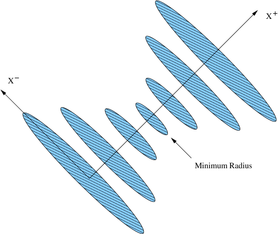
Figure 1: The circle radius shrinks to a minimum $L$ at $x^{+}=0$.

The basic structure of the space-time is depicted in figure 1. There is a circle whose radius shrinks as we increase $x^{+}$ until it reaches size $L$ at $x^{+}=0$. The size, $L$, is a tunable modulus in the metric. Viewing $x^{+}$ as light-cone time, we see that a particle becomes blue-shifted as time evolves by an amount that increases with decreasing $L$. The singular limit corresponds to taking $L\rightarrow 0$. The resulting singular space has been considered in [1]. From this perspective, the background is light-cone time-dependent.

The aim of this work is to find a DLCQ description of the null-brane. We should note that for non-zero $L$ this space-time has the following virtues. First, there are no pathologies: neither curvature singularities nor closed causal curves. Second, there is a null killing vector which facilitates string quantization. A space-time with these properties serves as a good perturbative string background with an S-matrix. Indeed, string scattering has been studied on this background [25, 2, 26]. However, on taking the limit $L\rightarrow 0$, the space-time develops a null singularity. This is an added feature that allows us to access the physics of a big crunch/big bang singularity in what we might hope is a controlled manner.

In section $2$, we define the null-brane quotient and study M-theory and string theory compactified on this background at the level of supergravity. In section $3$, we describe a decoupling limit that captures the DLCQ physics of the null-brane. In section $4$, we derive the Matrix description of M-theory on the null-brane for the case $N=1$ of a single D-brane using the DBI action. This model is already quite fascinating: it looks like a $1+1$-dimensional field theory on a cylinder whose radius is time-dependent. In the far past and the far future, the cylinder shrinks to zero size. The cylinder reaches a maximum radius at $x^{+}=0$ proportional to $1/L$ which diverges as $L\rightarrow 0$. This is quite reminiscent of the way in which Milne space appeared as the string worldsheet in [12]. It should be contrasted with the holographic description of branes wrapping the null-brane which gives a space-time-dependent non-commutative field theory [10].

We then proceed to conjecture the complete non-abelian answer for many branes using results based in part on the quotient description of the null-brane and in part on the DBI approach. We then present some additional arguments suggesting that our final Matrix Lagrangian is complete.

2 Defining the Background

2.1 The orbifold group

We define our background as follows: consider ${\mathbb{R}}^{1,3}$ parametrized by coordinates

$$x^{\pm}=\frac{1}{\sqrt{2}}(x^{0}\pm x^{1}),\,x,\,z,$$

with the usual metric $ds^{2}=-2dx^{+}dx^{-}+dx^{2}+dz^{2}$. We act on these coordinates by an element of the 4-dimensional Poincaré group:

$$g=\exp(2\pi iK);\quad K=\frac{\lambda}{\sqrt{2}}(J^{0x}+J^{1x})+LP^{z},$$ (1)

where $L$ has dimensions of length. This is the only scale beyond the Planck scale in our setup. Under this action which depends on $(\lambda,L)$,

$$X=\left(\begin{array}[]{c}x^{+}\\ x^{-}\\ x\\ z\\ \end{array}\right)\ \rightarrow\quad g\cdot X=\left(\begin{array}[]{c}x^{+}\\ x^{-}+2\pi\lambda x+2\pi^{2}\lambda^{2}x^{+}\\ x+2\pi\lambda x^{+}\\ z+2\pi L\\ \end{array}\right).$$ (2)

The parameter $\lambda$ can be set to one by a light-cone boost

$$x^{+}\rightarrow{x^{+}\over\lambda},\quad x^{-}\rightarrow\lambda x^{-}.$$ (3)

For most of our discussion, we will assume $\lambda=1$ except when we discuss decoupling in section 3.2. The length squared of closed curves can be easily computed,

$$\left(g^{n}\cdot X-X\right)^{2}=(2\pi nx^{+})^{2}+(2\pi nL)^{2}>0\ .$$ (4)

There are no closed causal curves. For sufficiently low energy scattering, we therefore need not worry about effects from large back reaction invalidating perturbative string computations.

It is worth stressing that four of the ten Poincaré generators are unbroken – those that commute with $K$. These are

$$P^{+},\quad P^{z},\quad K,\quad\widetilde{K}=\frac{1}{\sqrt{2}}(J^{0z}+J^{1z})+LP^{x}.$$

A quotient group element $g$ acts on the momenta in the following way:

$$P=\left(\begin{array}[]{c}p^{+}\\ p^{-}\\ p^{x}\\ p^{z}\\ \end{array}\right);\quad g\cdot P=\left(\begin{array}[]{c}p^{+}\\ p^{-}+2\pi p^{x}+2\pi^{2}p^{+}\\ p^{x}+2\pi p^{+}\\ p^{z}\\ \end{array}\right).$$ (5)

We note that for this orbifold, it is not the case that any point with $x^{+}<0$ is in the causal past of every point with $x^{+}>0$. To check this, we compute

$$\begin{array}[]{ccl}\left(X-g^{n}\cdot\tilde{X}\right)^{2}&=&-2\Delta x^{+}\Delta x^{-}+(\Delta x)^{2}+(2\pi n)^{2}x^{+}\tilde{x}^{+}+2(2\pi n)(x^{+}\tilde{x}-x\tilde{x}^{+})\\ &&+(\Delta z)^{2}-2(2\pi n)L\Delta z+(2\pi n)^{2}L^{2},\end{array}$$ (6)

where $\Delta x^{\mu}=x^{\mu}-\tilde{x}^{\mu}$. At large $n$, we have $(2\pi n)^{2}(x^{+}\tilde{x}^{+}+L^{2})$, so only points with $x^{+}\tilde{x}^{+}<-L^{2}$ are always causally related in this way.

The orbifold action lifts to the spin bundle over ${\mathbb{R}}^{1,3}$. To determine the number of preserved supersymmetries, we need to count the number of spinors, $\epsilon$, left invariant by (the lift of) $K$. The $P^{z}$ term in $K$ does not act on a spinor. In terms of standard real gamma matrices, $\Gamma^{\mu}$, satisfying the Clifford algebra relations,

$$\{\Gamma^{\mu},\Gamma^{\nu}\}=\eta^{\mu\nu},\quad\mu,\nu=0,\ldots,10,$$

it is easy to check that the invariance condition,

$$\left(\Gamma^{0x}+\Gamma^{1x}\right)\epsilon=0,$$ (7)

implies that

$$\Gamma^{+}\epsilon=0.$$ (8)

This background therefore preserves one-half of the available supersymmetry. To construct a string or M-theory background, we simply append an additional flat ${\mathbb{R}}^{6}$ or ${\mathbb{R}}^{7}$ factor to give a $10$ or $11$-dimensional metric.

2.2 The null-brane background

It is natural to express the metric in terms of new variables in which the quotient action simplifies. This choice of coordinates makes it easy to reduce along orbits of $K$. Let us perform the following change of variables:

$$\hat{x}^{+}=x^{+},\quad\hat{x}^{-}=x^{-}-{zx\over L}+{z^{2}x^{+}\over 2L^{2}},\quad\hat{x}=x-{zx^{+}\over L},\quad\hat{z}=\frac{z}{L}.$$ (9)

The hatted $x$-coordinates are natural because they are invariant under the action of $K$. The group element $g$ of equation $(\ref{gen})$ acts only by translation on $\hat{z}$ sending

$$\hat{z}\rightarrow\hat{z}+2\pi.$$

In these coordinates, the metric takes the form

$$ds^{2}=-2d\hat{x}^{+}d\hat{x}^{-}+d\hat{x}^{2}+((\hat{x}^{+})^{2}+L^{2})d\hat{z}^{2}+{2}(\hat{x}^{+}d\hat{x}-\hat{x}d\hat{x}^{+})d\hat{z}.$$ (10)

This metric was obtained by a coordinate change from flat space so there is no curvature.

2.3 M-theory on the null-brane

Let us consider M-theory on this space-time and reduce to type IIA on the $\hat{z}$ circle. We obtain a solution similar to a flux-brane, but with a null RR 1-form field strength. After massaging $(\ref{invmetric})$ into the standard form for determining the string metric, we see that the flat 11-dimensional metric becomes:

$$\begin{array}[]{ccl}ds_{11}^{2}&=&-2dx^{+}dx^{-}+dx^{2}+dz^{2}+(ds_{7})^{2}\\ &=&-2d\hat{x}^{+}d\hat{x}^{-}-{\hat{x}^{2}\over\Lambda}(d\hat{x}^{+})^{2}+{2\hat{x}\hat{x}^{+}\over\Lambda}d\hat{x}d\hat{x}^{+}+\Lambda\left(d\hat{z}+{\hat{x}^{+}\over\Lambda}d\hat{x}-{\hat{x}\over\Lambda}d\hat{x}^{+}\right)^{2}\\ &&+{L^{2}\over\Lambda}d\hat{x}^{2}+(ds_{7})^{2}\\ \end{array}$$ (11)

where

$$\Lambda=(\hat{x}^{+})^{2}+L^{2}.$$ (12)

To obtain the string frame metric, we use the usual relation

$$ds_{11}^{2}=e^{4\phi/3}(d\hat{z}+A)^{2}+e^{-2\phi/3}ds_{10}^{2}$$ (13)

where $ds_{10}^{2}$ is the string frame metric, and $A$ is the RR 1-form. Using this relation, we read off the following string metric, dilaton, and RR 1-form potential:

$$ds_{10}^{2} = \Lambda^{1/2}\left\{-2d\hat{x}^{+}d\hat{x}^{-}-{\hat{x}^{2}\over\Lambda}(d\hat{x}^{+})^{2}+{2\hat{x}\hat{x}^{+}\over\Lambda}d\hat{x}d\hat{x}^{+}+{L^{2}\over\Lambda}d\hat{x}^{2}+(ds_{7})^{2}\right\}$$ (14)

$$\phi = {3\over 4}\,{\rm log}\,\Lambda$$ (15)

$$A = \left({\hat{x}^{+}}d\hat{x}-{\hat{x}}d\hat{x}^{+}\right)/\Lambda.$$ (16)

The field strength $F$ associated to $A$ is null,

$$F={2L^{2}\over\Lambda^{2}}\,d\hat{x}^{+}\wedge d\hat{x},$$

which is the reason for the terminology “null-brane” given in [23]. Note that the string coupling becomes small at $\hat{x}^{+}=0$ when we take $L\rightarrow 0$.

2.4 Type II string theory on the null-brane

We now turn to type II string theory quotiented by the action $(\ref{quotgroup})$, or equivalently with the metric $(\ref{invmetric})$. We have no $B$-field and no RR fields. The dilaton is constant, $g_{s}=e^{\Phi_{0}}$. What happens as $L$ becomes small compared to the string scale? It seems wise to see what duality at the level of the supergravity solution can teach us.

In the limit where $L\rightarrow 0$, the metric develops a singularity at $\hat{x}^{+}=0$ which is basically the $\hat{z}$ circle shrinking to zero size resulting in a closed null curve. It is natural to therefore T-dualize along $\hat{z}$ which results in the metric (see, for example, [28])

$$ds_{\mathrm{T-dual}}^{2} = -2dx^{+}dx^{-}-\frac{x^{2}}{L^{2}+(x^{+})^{2}}(dx^{+})^{2}+2\frac{x^{+}x}{L^{2}+(x^{+})^{2}}dx^{+}dx$$ (18)

$$+\frac{L^{2}}{L^{2}+(x^{+})^{2}}dx^{2}+\frac{1}{L^{2}+(x^{+})^{2}}d\tilde{z}^{2}$$

where the T-dual coordinate $\tilde{z}$ still has a period of $2\pi$ (we use units where $\alpha^{\prime}=1$ for the moment). We have dropped the hats for the T-dual variables. There are also $B$-fields generated

$$B_{+\tilde{z}} = \frac{x}{L^{2}+(x^{+})^{2}},$$ (19)

$$B_{\tilde{z}x} = \frac{x^{+}}{L^{2}+(x^{+})^{2}},$$

and the dilaton is no longer constant,

$$\Phi = \Phi_{0}-\frac{1}{2}\ln\left(L^{2}+(x^{+})^{2}\right),$$

$$\tilde{g}_{s} = \frac{g_{s}}{\sqrt{L^{2}+(x^{+})^{2}}}.$$ (20)

The first thing to note is that if we hold $g_{s}$ fixed and take $L\rightarrow 0$, the dual coupling diverges at $x^{+}=0$. From the original quotient group perspective, this corresponds to going over to the parabolic orbifold studied in [29, 1].

The $B$-field gives a field strength whose only non-vanishing component is

$$H_{+x\tilde{z}}=-\frac{2L^{2}}{\left(L^{2}+(x^{+})^{2}\right)^{2}}.$$ (21)

This field strength diverges as $L\rightarrow 0$ at $x^{+}\rightarrow 0$. This is intriguing and suggests the existence of a kind of critical theory of closed strings in a large light-light $B$-field. There is a strong analogy with open strings in a light-like constant 2-form field strength, and there might well be a relation with the non-relativistic strings studied in [27]. The metric $(\ref{tdualmet})$ is now curved with non-vanishing curvature components:

$$R_{+\tilde{z}+}\vphantom{R}^{\tilde{z}}=\frac{L^{2}-2(x^{+})^{2}}{\left(L^{2}+(x^{+})^{2}\right)^{2}},\qquad\qquad R_{+x+}\vphantom{R}^{x}=\frac{3L^{2}}{\left(L^{2}+(x^{+})^{2}\right)^{2}},$$ (22)

$$R_{+x+}\vphantom{R}^{-}=\frac{3L^{2}x^{+}x}{\left(L^{2}+(x^{+})^{2}\right)^{3}},\qquad\qquad R_{+xx}\vphantom{R}^{-}=\frac{3L^{4}}{\left(L^{2}+(x^{+})^{2}\right)^{3}},$$

$$R_{++}=\frac{4L^{2}-2(x^{+})^{2}}{\left(L^{2}+(x^{+})^{2}\right)^{2}},\qquad\qquad R=0.$$

It is not hard to check that this dilaton, $H$-field and Ricci tensor combine to give a good string background with vanishing beta functions as we expect. It is also worth noting that as $L\rightarrow 0$ with $x^{+}\gg L$, $H\rightarrow 0$, but the string coupling and curvature are still nontrivial:

$$\tilde{g}_{s}\rightarrow{g_{s}\over|x^{+}|},\qquad\qquad R_{++}\rightarrow-{2\over(x^{+})^{2}}.$$ (23)

Finally, we would like to lift this configuration to M-theory. This is natural if we consider type IIA on the metric $(\ref{tdualmet})$, and we choose to hold $g_{s}$ fixed but consider $L\rightarrow 0$. Let $y$ denote the coordinate of the M-theory circle, we then obtain the following $11$-dimensional solution:

$$ds_{11}^{2} = (g_{s})^{-\frac{2}{3}}\left\{L^{2}+(x^{+})^{2}\right\}^{\frac{1}{3}}ds_{\mathrm{T-dual}}^{2}+(g_{s})^{\frac{4}{3}}\left\{L^{2}+(x^{+})^{2}\right\}^{-\frac{2}{3}}dy^{2},$$

$$= \left(g_{s}\{L^{2}+(x^{+})^{2}\}\right)^{-\frac{2}{3}}\left[-2\left\{L^{2}+(x^{+})^{2}\right\}dx^{+}dx^{-}-x^{2}(dx^{+})^{2}\right.$$

$$\left.\vphantom{\left(L^{2}+(x^{+})^{2}\right)}+2x^{+}xdx^{+}dx+L^{2}dx^{2}+d\tilde{z}^{2}+g_{s}^{2}dy^{2}\right],$$

and a longitudinal 3-form potential,

$$C_{+\tilde{z}y} = \frac{2}{3}\frac{x}{L^{2}+(x^{+})^{2}},$$ (25)

$$C_{\tilde{z}xy} = \frac{2}{3}\frac{x^{+}}{L^{2}+(x^{+})^{2}},$$

with 4-form field strength

$$G_{+x\tilde{z}y}=-\frac{4}{3}\frac{L^{2}}{\left\{L^{2}+(x^{+})^{2}\right\}^{2}}.$$ (26)

The curvature of the metric can be computed. We will quote only the Ricci tensor whose non-vanishing component is

$$R_{++}=\frac{8L^{2}-12(x^{+})^{2}}{\left\{L^{2}+(x^{+})^{2}\right\}^{2}}.$$ (27)

The Ricci scalar vanishes as before. Lastly, note that had we considered type IIB on $(\ref{tdualmet})$, it would have been natural to use S-duality when the coupling becomes large.

3 The DLCQ Description

3.1 Light-like to space-like compactification

We first note that the action of $p^{+}$ commutes with the null-brane quotient $(\ref{quotgroup})$. This means we can compactify the $\hat{x}^{-}$ direction,

$$\hat{x}^{-}\sim\hat{x}^{-}+R,$$ (28)

and consider the sector with fixed light-cone momentum ${\hat{p}}^{+}=N/R$.

We cannot relate this light-like compactification to a space-like compactification using the procedure of [30] because the metric $(\ref{invmetric})$ depends explicitly on $\hat{x}^{+}$. However, we can use the modified procedure of [12]. Choose a direction ${\hat{x}}^{1}$ and make the identifications

$$\left(\hat{x}^{+},\hat{x}^{-},{\hat{x}}^{1}\right)\sim\left(\hat{x}^{+},\hat{x}^{-},{\hat{x}}^{1}\right)+\left(0,R,\epsilon R\right).$$ (29)

The Lorentz transformation

$$\hat{x}^{+}=X^{+},\qquad\hat{x}^{-}={X^{+}\over 2\epsilon^{2}}+{X^{-}}+{{X}^{1}\over\epsilon},\qquad{\hat{x}}^{1}={X^{+}\over\epsilon}+X^{1},\qquad\hat{x}^{i}=X^{i}\quad i>1,$$ (30)

while holding fixed $L$ and

$$z={Z},$$ (31)

results in the M-theory metric

$$ds_{11}^{2}=-2dX^{+}dX^{-}+dX^{2}+\left((X^{+})^{2}+L^{2}\right)dZ^{2}+2\left(X^{+}dX-XdX^{+}\right)dZ+\sum_{i=1}^{7}(dX^{i})^{2}$$ (32)

with the identifications

$$Z\sim Z+2\pi,\qquad X^{1}\sim X^{1}+\epsilon R.$$ (33)

There are $N$ units of momentum in the $X^{1}$ direction.

We reduce to type IIA on the $X^{1}$ circle. This is a straightforward reduction which leaves us with type IIA on a space with metric

$$ds_{10}^{2}=-2dX^{+}dX^{-}+dX^{2}+\left((X^{+})^{2}+L^{2}\right)dZ^{2}+2\left(X^{+}dX-XdX^{+}\right)dZ+\sum_{i=2}^{7}(dX^{i})^{2}$$ (34)

and $N$ D0-branes. This is the theory of $N$ D0-branes on the null-brane quotient.

We can also arrive at this same conclusion by directly studying the orbifold action $(\ref{quotgroup})$. It is easy to check that the identification

$$\left(x^{+},x^{-},{x}^{1}\right)\sim\left(x^{+},x^{-},{x}^{1}\right)+\left(0,R,\epsilon R\right)$$ (35)

commutes with the orbifold action. After making the same Lorentz transformation given in $(\ref{Lorentz})$, the DLCQ identification becomes

$$X^{1}\sim X^{1}+\epsilon R.$$ (36)

Using either approach, we reduce the study of the light-like compactified null-brane in M-theory to the study of the dynamics of $N$ D0-branes on the null-brane quotient. Our task in section 4 is to determine this theory.

3.2 A decoupling limit

Note, however, that this procedure does not result in a decoupling limit because the transformation $(\ref{Lorentz})$ does not involve a rescaling of $\hat{x}^{+}$ so the corresponding light-cone energy $\hat{p}^{-}$ does not become small.

To obtain a decoupling limit, we need to perform an additional transformation. Let us return to the orbifold description $(\ref{quotgroup})$ with $\lambda$ a free parameter. First note that the identification $(\ref{twisted})$ implies that

$$p^{+}=\epsilon p^{1}$$ (37)

if we stay in the DLCQ sector with fixed $N$.

The Lorentz transformation $(\ref{Lorentz})$ applied to the flat space variables takes us to a space-like circle but does not scale the light-cone energy $E^{-}$. Rather the energy and momenta transform in the following way

$$E^{-}\rightarrow E^{-}+{p^{+}\over 2\epsilon^{2}}-{p^{1}\over\epsilon},\qquad p^{+}\rightarrow p^{+},\qquad p^{1}\rightarrow p^{1}-{p^{+}\over\epsilon}.$$ (38)

The mass shell condition,

$$-2E^{-}p^{+}+p^{i}p_{i}+m^{2}=0,$$ (39)

together with the relation $(\ref{relationship})$ implies that $p^{i}\sim O(\epsilon)$ while $p^{+}\sim O(\epsilon^{2})$ and $E^{-}\sim O(1)$. The null-brane quotient determined by $\lambda$ is unchanged but $X^{1}$ satisfies the condition $(\ref{spacelike})$.

We now boost to rescale our energies sending

$$X^{+}\rightarrow\epsilon X^{+},\quad X^{-}\rightarrow{X^{-}\over\epsilon}.$$ (40)

This has the effect of sending $\lambda\rightarrow\epsilon\lambda$ while leaving $L$ invariant. All energies and momenta are now of order $\epsilon$. Reducing to type IIA string theory on $X^{1}$ gives us type IIA string theory with

$$g_{s}\sim\epsilon^{3/2},\quad\ell_{s}\sim\epsilon^{-1/2}$$ (41)

and a flat metric quotiented by the null-brane identification with parameters $(\lambda,L)$ where $\lambda\sim\epsilon$.

We can now change to invariant coordinates using $(\ref{hatted})$ now including factors of $\lambda$. It is easy to find the resulting metric

$$ds^{2}=-2d\hat{x}^{+}d\hat{x}^{-}+d\hat{x}^{2}+(\{\lambda\hat{x}^{+}\}^{2}+L^{2})d\hat{z}^{2}+{2\lambda}(\hat{x}^{+}d\hat{x}-\hat{x}d\hat{x}^{+})d\hat{z}+d\hat{x}^{i}d\hat{x}^{i}.$$ (42)

By rescaling $\hat{z}$, we see that this metric really depends on the combination $L/\epsilon\lambda$. For the moment, however, we choose to keep $\hat{z}$ dimensionless with canonical period $2\pi$. These scalings define a decoupling limit for M-theory on the null-brane quotient. String oscillators decouple because our characteristic energy $\epsilon E^{-}$ is much smaller than the string scale given in $(\ref{scales})$. Closed strings also decouple because the 10-dimensional Newton constant is becoming small at these energies,

$$g_{s}^{2}\left({\epsilon E^{-}\ell_{s}}\right)^{8}\rightarrow 0,$$

as $\epsilon\rightarrow 0$. We will apply these scalings to the theory of D0-branes on the null-brane in the following section.

4 D-branes on the null-brane

4.1 Decoupling the DBI action

An analysis of boundary states in the null-brane appears in [31]. Our goal in this section is to derive the gauge theory describing the dynamics of $N$ D0-branes on the null-brane. The natural approach to use is the orbifold description of the null-brane given by the identification $(\ref{quotgroup})$. This turns out to be subtle for reasons we will describe later. Therefore, we first consider the abelian case with $N=1$ where we can use the DBI action.

We start with type IIA string theory with a single D0-brane moving on a space-time with metric $(\ref{newmetric})$ where, for the moment, we do not decouple. A T-duality along $\hat{z}$ converts the D0-brane to a D-string wrapped along the T-dual direction $z$. On performing this T-duality, we find

$$ds^{2} = -\frac{\lambda^{2}x^{2}}{\Lambda}(dx^{+})^{2}-2dx^{+}dx^{-}+\frac{2\lambda^{2}x^{+}x}{\Lambda}dx^{+}dx+\frac{L^{2}}{\Lambda}dx^{2}+\frac{(\alpha^{\prime})^{2}}{\Lambda}dz^{2}+dx^{i}dx^{i},$$

$$B = \frac{2\alpha^{\prime}}{\Lambda}\left(-xdx^{+}+x^{+}dx\right)\wedge dz,$$

$$e^{2\Phi} = \frac{\alpha^{\prime}g_{s}^{2}}{\Lambda},$$ (43)

where

$$\Lambda=L^{2}+\lambda^{2}(x^{+})^{2},$$ (44)

and $z$ is again dimensionless with period $2\pi$.

The DBI action is given by

$$S=-\frac{1}{\alpha^{\prime}}\int d\tau d\sigma e^{-\Phi}\sqrt{-\det\left[\left(G_{\mu\nu}+B_{\mu\nu}\right)\partial_{a}X^{\mu}\partial_{b}X^{\nu}+2\pi\alpha^{\prime}F_{ab}\right]}.$$ (45)

Evaluating this action on the solution $(\ref{DBIback})$ gives

$$S= -\frac{1}{g_{s}(\alpha^{\prime})^{\frac{3}{2}}}\int d\tau d\sigma\left\{-\Lambda\left[\left(-\frac{\lambda^{2}x^{2}}{\Lambda}(\dot{x}^{+})^{2}-2\dot{x}^{+}\dot{x}^{-}+\frac{2\lambda^{2}x^{+}x}{\Lambda}\dot{x}^{+}\dot{x}+\frac{L^{2}}{\Lambda}\dot{x}^{2}+\frac{(\alpha^{\prime})^{2}}{\Lambda}\dot{z}^{2}+\dot{x}^{i}\dot{x}^{i}\right)\right.\right.$$ (46)

$$\left.\left.\times\left(-\frac{\lambda^{2}x^{2}}{\Lambda}(x^{+\prime})^{2}-2x^{+\prime}x^{-\prime}+\frac{2\lambda^{2}x^{+}x}{\Lambda}x^{+\prime}x^{\prime}+\frac{L^{2}}{\Lambda}(x^{\prime})^{2}+\frac{(\alpha^{\prime})^{2}}{\Lambda}(z^{\prime})^{2}+x^{i\prime}x^{i\prime}\right)\right.\right.$$

$$\left.\left.-\left(-\frac{\lambda^{2}x^{2}}{\Lambda}\dot{x}^{+}x^{+\prime}-\dot{x}^{+}x^{-\prime}-\dot{x}^{-}x^{+\prime}+\frac{\lambda^{2}x^{+}x}{\Lambda}\dot{x}^{+}x^{\prime}+\frac{\lambda^{2}x^{+}x}{\Lambda}\dot{x}x^{+\prime}+\frac{L^{2}}{\Lambda}\dot{x}x^{\prime}+\frac{(\alpha^{\prime})^{2}}{\Lambda}\dot{z}z^{\prime}+\dot{x}^{i}x^{i\prime}\right)^{2}\right.\right.$$

$$\left.\left.+\left(-\frac{\lambda\alpha^{\prime}x}{\Lambda}\dot{x}^{+}z^{\prime}+\frac{\lambda\alpha^{\prime}x}{\Lambda}\dot{z}x^{+\prime}+\frac{\lambda\alpha^{\prime}x^{+}}{\Lambda}\dot{x}z^{\prime}-\frac{\lambda\alpha^{\prime}x^{+}}{\Lambda}\dot{z}x^{\prime}+2\pi\alpha^{\prime}F\right)^{2}\right]\right\}^{\frac{1}{2}}.$$

Note that a prime denotes a $\sigma$ derivative while a dot denotes a $\tau$ derivative. We now make the gauge choice

$$z=\sigma$$ (47)

so $\sigma$ has period $2\pi$. The action $(\ref{largeexp})$ simplifies to:

$$S=-\frac{1}{g_{s}(\alpha^{\prime})^{\frac{3}{2}}}\int d\tau d\sigma \big{\{}(\alpha^{\prime})^{2}\big{[}\left(2\dot{x}^{+}\dot{x}^{-}-\dot{x}^{2}-\dot{x}^{i}\dot{x}^{i}\right)+4\pi\lambda F\left(x\dot{x}^{+}-x^{+}\dot{x}\right)$$ (49)

$$-4\pi^{2}\Lambda F^{2}\big{]}+\ldots\big{\}}^{\frac{1}{2}},$$

where the dots represent terms that are either sixth order in the $x^{\mu}$, or are $L^{2}$ times something fourth order in $x^{\mu}$, each with precisely two $\tau$ derivatives and two $\sigma$ derivatives.

Next we use our gauge freedom to set

$$x^{+}=c\tau/\sqrt{2}$$ (50)

where $c$ is a constant. We expand around the static configuration $x^{+}=x^{-}=c\tau/\sqrt{2}$ by substituting $x^{-}=c\tau/\sqrt{2}+\sqrt{2}y$ where $y$ is a fluctuation. The result is

$$S = -\frac{1}{g_{s}(\alpha^{\prime})^{\frac{3}{2}}}\int d\tau d\sigma\left\{(\alpha^{\prime})^{2}\left[\left(c^{2}+2c\dot{y}-\dot{x}^{2}-\dot{x}^{i}\dot{x}^{i}\right)+2\sqrt{2}\pi\lambda cF\left(x-\tau\dot{x}\right)-4\pi^{2}\Lambda F^{2}\right]\right.$$

$$\left.+\frac{1}{2}\lambda^{2}c^{2}x^{2}(x^{\prime})^{2}+L^{2}c^{2}(x^{\prime})^{2}+2L^{2}c\dot{y}(x^{\prime})^{2}-L^{2}\dot{x}^{i}\dot{x}^{i}(x^{\prime})^{2}+\frac{1}{2}\lambda^{2}c^{2}x^{2}x^{i\prime}x^{i\prime}\right.$$

$$\left.+c^{2}\Lambda x^{i\prime}x^{i\prime}+2c\Lambda\dot{y}x^{i\prime}x^{i\prime}-\lambda^{2}c^{2}\tau x\dot{x}x^{i\prime}x^{i\prime}-L^{2}\dot{x}^{2}x^{i\prime}x^{i\prime}-\Lambda\dot{x}^{i}\dot{x}^{i}x^{j\prime}x^{j\prime}+c^{2}\Lambda(y^{\prime})^{2}\right.$$

$$\left.-\lambda^{2}c^{3}\tau xy^{\prime}x^{\prime}-2L^{2}c\dot{x}y^{\prime}x^{\prime}-2c\Lambda\dot{x}^{i}y^{\prime}x^{i\prime}+\lambda^{2}c^{2}\tau x\dot{x}^{i}x^{\prime}x^{i\prime}+2L^{2}\dot{x}\dot{x}^{i}x^{\prime}x^{i\prime}+\Lambda\dot{x}^{i}\dot{x}^{j}x^{i\prime}x^{j\prime}\right\}^{\frac{1}{2}}.$$

We can now apply the decoupling limit discussed in section 3.2. In this limit, our parameters scale as follows:

$$g_{s}(\alpha^{\prime})^{\frac{3}{2}} \rightarrow g_{s}(\alpha^{\prime})^{\frac{3}{2}},$$

$$\alpha^{\prime} \rightarrow \epsilon^{-1}\alpha^{\prime},$$ (52)

$$\lambda \rightarrow \epsilon\lambda.$$

In this decoupling limit, our space-time energy $E^{-}$ is $O(\epsilon)$. We want to consider energies of $O(1)$ in this gauge theory so in $(\ref{defc})$, we choose $c=1/\lambda$ which scales like $\epsilon^{-1}$. Energies with respect to this choice of world-volume time $\tau$ are finite. With these choices, we find that

$$S = -\frac{1}{g_{s}\sqrt{\alpha^{\prime}}}\int d\tau d\sigma\left\{\frac{1}{\epsilon^{2}}+\frac{1}{\epsilon}\dot{y}-\frac{1}{2}\left(\dot{y}^{2}+\dot{x}^{2}+\dot{x}^{i}\dot{x}^{i}\right)+\sqrt{2}\pi\left(x-\tau\dot{x}\right)F-2\pi^{2}\Lambda F^{2}\right.$$ (53)

$$\left.+\frac{1}{2(\alpha^{\prime})^{2}}\left(L^{2}(x^{\prime})^{2}+\Lambda\left((y^{\prime})^{2}+x^{i\prime}x^{i\prime}\right)\right)+\mathcal{O}(\epsilon)\right\},$$

now written in terms of non-scaling quantities. Note that $\Lambda=\frac{1}{2}\tau^{2}+L^{2}$ is finite. We can drop the first two terms (a constant and a total $\tau$ derivative), and the omitted higher terms which vanish when $\epsilon\rightarrow 0$ leaving an action which does not scale.

The dimension assignments in $(\ref{redaction})$ are as follows: the scalar fields $y$, $x$, $x^{i}$ have length dimension one, as does $\tau$ while $\sigma$ is dimensionless. $A_{\tau}$ has mass dimension one, while $A_{\sigma}$ is dimensionless so that $F$ has uniform mass dimension one. We will rescale these fields to assign canonical dimensions after discussing the non-abelian generalization. Note that the $SO(6)$ symmetry acting on the $x^{i}$ is enhanced to an $SO(7)$ acting on $(x^{i},y)$.

4.2 A non-abelian generalization

Although we used the DBI action to find the DLCQ description for the $N=1$ case, the natural approach would have been to employ the orbifold description of the null-brane given by the identification $(\ref{quotgroup})$. Because the quotient action involves a boost, we will meet some interesting subtleties in trying to use this approach.

Let us try to proceed straightforwardly: to describe the theory of $N$ D-branes on the null-brane, we go to the covering space of the quotient group action $\Gamma={\mathbb{Z}}$, and consider a collection of $(N\times|\Gamma|)\times(N\times|\Gamma|)$ matrices $X^{\mu}$. The $|\Gamma|=\infty$ label indexes the image branes needed to assure invariance under the quotient action. In fact, these matrices can be viewed as operators on a Hilbert space $\mathcal{H}=\Gamma\otimes\mathbb{C}^{N}$. This picture will be useful below when we want to do a Fourier transformation to a new basis for $\mathcal{H}$.

There are $\operatorname{U}(N\times|\Gamma|)$ gauge transformations that act on these matrices. We must impose certain constraints both on the matrices $X^{\mu}$ as well as on the gauge transformations to ensure that everything is invariant under the quotient action.

Let us first ignore dynamics and treat the Euclidean D-brane problem, or equivalently the pure matrix problem. To implement the invariance constraints, let us first define partial matrix elements $X^{\mu}_{mn}=\langle m|X^{\mu}|n\rangle$ which are $N\times N$ Hermitian matrices. Now the action of the $k^{th}$ quotient group element is easy to understand. Since the group element acts by the representation $\rho$ where $\rho(k)|n\rangle=|n+k\rangle$, we see that

$$\left(\rho(k)^{\dagger}X^{\mu}\rho(k)\right)_{mn}=X^{\mu}_{m+k,n+k}.$$

The constraints on the matrices then become

$$X_{m+k,n+k}^{+,i} = X_{mn}^{+,i},$$

$$X_{m+k,n+k} = X_{mn}+2\pi kX_{mn}^{+},$$ (54)

$$X_{m+k,n+k}^{-} = X_{mn}^{-}+2\pi kX_{mn}+2\pi^{2}k^{2}X_{mn}^{+},$$

$$Z_{m+k,n+k} = Z_{mn}+2\pi kL\delta_{mn}.$$

The residual gauge transformations are the elements of $\operatorname{U}(N\times|\Gamma|)$ which commute with $\rho(k)$ for all $k$. Using notation similar to that used above, this simply says that we restrict to unitary matrices $U$ satisfying $U_{m+k,n+k}=U_{mn}$. The action constructed from these matrices is the usual one,

$$S={1\over 4g_{s}(\alpha^{\prime})^{2}}\,\operatorname{Tr}\left[X^{\mu},X^{\nu}\right]^{2}.$$ (55)

If we were to study Euclidean D0-branes or D-instantons on the null-brane then we would proceed to solve these pure matrix constraints. The solution of these constraints is presented in Appendix A. We, however, would like to describe dynamical branes. This involves an identification of world-volume time, $\tau$, with a space-time coordinate. Conventional static gauge corresponds to the choice,

$$x^{0}={\tau}.$$ (56)

This choice, however, leads to a theory that involves image branes shifted in time. So in accord with our prior DBI analysis, let us consider the gauge choice

$$x^{+}={{\tau}\over\sqrt{2}}.$$ (57)

With respect to this choice, each image brane is located at the same point in world-volume time. So we can consider a natural (but by no means unique) lift of the closed string orbifold identification $(\ref{quotgroup})$ to dynamical D-branes given by

$$X_{m+k,n+k}^{+,i} = X_{mn}^{+,i},$$ (58)

$$X_{m+k,n+k} = X_{mn}+\sqrt{2}\pi k\lambda{\tau}\delta_{mn},$$ (59)

$$X_{m+k,n+k}^{-} = X_{mn}^{-}+2\pi k\lambda X_{mn}+\sqrt{2}\pi^{2}k^{2}\lambda^{2}{\tau}\delta_{mn},$$ (60)

$$Z_{m+k,n+k} = Z_{mn}+2\pi kL\delta_{mn}.$$

We can follow the same procedure described in Appendix A to transition from an infinite-dimensional quantum mechanics system to a $1+1$-dimensional field theory where the fields depend on $(\tau,\theta)$ and $0\leq\theta\leq 1$. Note that $\theta$ is dimensionless but $L$ as well as $\tau$ and $X^{\mu}$ have length dimension $1$.

Following Appendix A and performing the Fourier transformation to $\theta$, we obtain

$$X^{+} = x^{+},$$

$$X = \widetilde{x}+i{\tau\over\sqrt{2}}\lambda\partial_{\theta},$$

$$X^{-} = {\widetilde{x}}^{-}+\frac{i}{2}\lambda{\widetilde{x}}^{\prime}+i{\widetilde{x}}\lambda\partial_{\theta}-{1\over 2\sqrt{2}}{\tau\lambda^{2}}\partial_{\theta}^{2},$$ (61)

$$Z = z+iL\partial_{\theta},$$

$$X^{i} = x^{i},$$

where small letters represent Hermitian operators that are functions of $(\tau,\theta)$, and a prime denotes a derivative with respect to $\theta$. Note that ${\widetilde{x}}^{-}$ has been defined so that it is Hermitian.

Gauge transformations, parametrized by a unitary $N\times N$ function $u$ of the variables $(\theta,\tau)$, act in the following way

$$x^{+}\rightarrow ux^{+}u^{\dagger},$$

$${\widetilde{x}}\rightarrow u{\widetilde{x}}u^{\dagger}+i{\tau\over\sqrt{2}}\lambda u{u^{\prime}}^{{\dagger}},$$

$${\widetilde{x}}^{-}\rightarrow u{\widetilde{x}}^{-}u^{\dagger}+\frac{i}{2}\lambda\left(u{\widetilde{x}}{u^{\prime}}^{{\dagger}}-u^{\prime}{\widetilde{x}}u^{\dagger}\right)+{1\over 2\sqrt{2}}\tau\lambda^{2}u^{\prime}{u^{\prime}}^{{\dagger}},$$

$$z\rightarrow uzu^{\dagger}+iLu{u^{\prime}}^{{\dagger}},$$

$$x^{i}\rightarrow ux^{i}u^{\dagger}.$$

Gauge covariant combinations are given by a transformation similar to $(\ref{hatted})$

$$x= {\widetilde{x}}-\frac{\tau\lambda}{\sqrt{2}L}z,$$

$${x}^{-}= {\widetilde{x}}^{-}-\frac{\lambda}{2L}\left\{{\widetilde{x}},z\right\}+\frac{\tau\lambda^{2}}{2\sqrt{2}L^{2}}z^{2}.$$

In terms of these gauge covariant variables, the above operators are given by

$$X = x+{i\over\sqrt{2}}{\tau\lambda}D_{1},$$ (64)

$$X^{-} = x^{-}+\frac{i}{2}\lambda\left\{x,D_{1}\right\}-{1\over 2\sqrt{2}}{\tau\lambda^{2}}D_{1}^{2},$$ (65)

$$Z = iLD_{1}$$

where $D_{1}=\partial_{\theta}-{i\over L}z$.

There is, however, a rather crucial difference from the Euclidean case considered in Appendix A. We have necessarily treated $X^{+}$ asymmetrically in $(\ref{1constraints})$ versus $(\ref{2constraints})$ and $(\ref{3constraints})$. On the other hand, $X^{+}$ is treated uniformly in $(\ref{matconstraints})$ which leads to rather critical cancellations in the resulting Euclidean action $(\ref{action})$.

In static situations, we transition from D-instantons to D0-branes by making the replacement

$${X^{0}}\,\rightarrow\,\alpha^{\prime}iD^{0}=\alpha^{\prime}\left(i\partial_{\tau}+A^{0}\right).$$

However, following this approach using the action $(\ref{action})$ in this time-dependent case leads to a problematic action precisely because of the asymmetric treatment of $X^{+}$. Instead we can try to postulate a replacement of $\sqrt{2}x^{+}$ by $\tau+y$ and of $\sqrt{2}x^{-}$ by $\tau-y$. This will generate neither gauge-field terms nor kinetic terms for the fields but it does give the remaining interactions. Applying the decoupling limit $(\ref{resc})$ and sending $\tau\rightarrow\tau/\epsilon$ shows us that $X^{-}$ given in $(\ref{minkop})$ collapses to $x^{-}$. Then setting the rescaled $\lambda=1$ and computing commutators while retaining only terms independent of $\epsilon$ gives

$$\left[X^{+},X\right] = \frac{1}{\sqrt{2}}\left[y,x\right]-\frac{i\tau}{2}D_{1}y,$$

$$\left[X^{+},X^{-}\right] = 0,$$

$$\left[X^{+},Z\right] = -\frac{i}{\sqrt{2}}LD_{1}y,$$ (66)

$$\left[X^{+},X^{i}\right] = \frac{1}{\sqrt{2}}\left[y,x^{i}\right],$$

$$\left[X,X^{-}\right] = \frac{1}{\sqrt{2}}\left[y,x\right]-\frac{i\tau}{2}D_{1}y,$$

$$\left[X,Z\right] = -iLD_{1}x,$$

$$\left[X,X^{i}\right] = \left[x,x^{i}\right]+i{\tau\over\sqrt{2}}D_{1}x^{i},$$

$$\left[X^{-},Z\right] = \frac{iL}{\sqrt{2}}D_{1}y,$$

$$\left[X^{-},X^{i}\right] = -\frac{1}{\sqrt{2}}\left[y,x^{i}\right],$$

$$\left[Z,X^{i}\right] = iLD_{1}x^{i},$$

$$\left[X^{i},X^{j}\right] = \left[x^{i},x^{j}\right].$$

where we have defined covariant derivatives, e.g. $D_{0}x=[D_{0},x]$, and a field strength, $F=i[D_{0},D_{1}]$. The action can then be expressed in terms of the commutators $(\ref{ecomm})$

$$S ={1\over 2g_{s}(\alpha^{\prime})^{5/2}}\int d\theta d\tau\,\operatorname{Tr}\Big{(}-L^{2}(D_{1}x^{i})^{2}-L^{2}(D_{1}y)^{2}-L^{2}(D_{1}x)^{2}+\frac{1}{2}\left[x^{i},x^{j}\right]^{2}+\left[y,x^{i}\right]^{2}$$ (68)

$$+(\left[x,x^{i}\right]+{i\tau\over\sqrt{2}}D_{1}x^{i})^{2}+(\left[x,y\right]+{i\tau\over\sqrt{2}}D_{1}y)^{2}+\ldots\Big{)}.$$

The omitted terms involve either time derivatives or gauge-field strengths neither of which are generated by this ansatz. We are also omitting the fermion couplings. Note that, as in the abelian case, $y$ appears symmetrically with the $x^{i}$ while $x$ is distinguished.

We can now combine these couplings with our abelian action $(\ref{redaction})$ to arrive at a conjecture for the complete non-abelian DLCQ description of the null-brane. Since all the parameters are now finite, we can rescale $\theta$ by a factor of $\sqrt{\alpha^{\prime}}$ to length dimension $1$, rescale all the fields to canonical mass dimension $1$, and define $g^{2}_{YM}=g_{s}/\alpha^{\prime}$. We can finally set $\alpha^{\prime}=1$ for convenience and send $F\rightarrow 2\pi F$. The resulting action is

$$S ={1\over 2g_{YM}^{2}}\int d\theta d\tau\,\operatorname{Tr}\Big{(}(D_{0}x^{i})^{2}+(D_{0}y)^{2}+(D_{0}x)^{2}-L^{2}(D_{1}x^{i})^{2}-L^{2}(D_{1}y)^{2}-L^{2}(D_{1}x)^{2}$$ (71)

$$-\sqrt{2}(x-\tau D_{0}x)F+(L^{2}+\frac{1}{2}\tau^{2})F^{2}+\frac{1}{2}\left[x^{i},x^{j}\right]^{2}+\left[y,x^{i}\right]^{2}$$

$$+(\left[x,x^{i}\right]+{i\tau\over\sqrt{2}}D_{1}x^{i})^{2}+(\left[x,y\right]+{i\tau\over\sqrt{2}}D_{1}y)^{2}+{\rm fermions}\Big{)}.$$

Note that $(x^{i},y)$ are rotated by an $SO(7)$ symmetry and therefore should be combined.

There is another argument that there are no couplings beyond those seen in $(\ref{conjecture})$. D0-brane dynamics in flat space should be governed by a matrix quantum mechanics with an action given covariantly by

$$S=\frac{1}{2g_{YM}^{2}}\int d\tau\,\operatorname{Tr}\Big{(}\eta_{\mu\nu}D_{0}X^{\mu}D_{0}X^{\nu}+\frac{1}{2}\left[X^{\mu},X^{\nu}\right]\left[X_{\mu},X_{\nu}\right]+{\rm fermions}\Big{)}.$$ (72)

After substituting $(\ref{minkop})$ with $\sqrt{2}x^{\pm}=\tau\pm y$, the kinetic term gives

$$(D_{0}X^{\mu})^{2} = -\frac{1}{\epsilon^{2}}+(D_{0}x)^{2}+(D_{0}y)^{2}+(D_{0}x^{i})^{2}+(L^{2}+\frac{1}{2}\tau^{2})F^{2}$$ (74)

$$+\frac{1}{\sqrt{2}}\left(\tau\left\{D_{0}x,F\right\}-\left\{x,F\right\}\right)+\mathcal{O}(\epsilon).$$

After dropping the constant piece and tracing (which now includes an integration over $\theta)$, the result agrees precisely with the expression given above in $(\ref{conjecture})$. The contribution coming from squares of commutators is the same as before and so automatically agrees.

There are a few points worth emphasizing: first, a large gauge transformation along the $\theta$ circle simply implements the shift

$$z\rightarrow z+2\pi L.$$ (75)

In terms of the original variables and their gauge transformation properties given in $(\ref{noninvgt})$, this large gauge transformation implements the quotient identification. This Lagrangian $(\ref{conjecture})$ describes M-theory on the null-brane. However, in agreement with the supergravity solution $(\ref{stringmetric})$, the model is described by a kind of Matrix string theory [32, 33, 34] near $\tau=0$. On the other hand, as $|\tau|\rightarrow\infty$, fluctuations in $\theta$ are suppressed and the model reduces to quantum mechanics. A detailed study of the dynamics of this model will appear elsewhere.

If we wish to describe perturbative string theory on the null-brane then we need to compactify additional directions in the usual way [35] and study higher dimensional generalizations of $(\ref{conjecture})$. This is particularly interesting for type IIB string theory on the null-brane since the conventional IIB Matrix description [36] is promoted from a $2+1$ to a $3+1$-dimensional field theory. Lastly, we note that studying D-branes on this kind of quotient space gives a theory that should be closely connected to the dipole models of [37], perhaps with a time-dependent dipole. It would be interesting to make this connection precise.

Appendix A Euclidean D0-branes on the Null-brane

In this Appendix, we solve the matrix constraints $(\ref{matconstraints})$ to obtain an action for Euclidean D0-branes or D-instantons probing the null-brane. This action has been independently obtained recently in [9]. We should note that the analytic continuation to Euclidean space needed to describe D-instanton configurations is not straightforward for the null-brane. It is unclear whether physical amplitudes in type II string theory can really receive quantum corrections from these kinds of D-instantons. For us, however, the solution of the pure matrix problem is an intermediate step on the road to describing dynamical D-branes.

We wish to solve the pure matrix constraints $(\ref{matconstraints})$. Solving these constraints allows one to express the matrices $X^{\mu}_{mn}$ in terms of just $X^{\mu}_{m0}$. These latter matrices are the residual degrees of freedom. A more convenient picture is obtained by changing basis, from $|n\rangle$ to

$$|\theta\rangle=\sum_{k}e^{2\pi ik\theta}|k\rangle,$$ (76)

where now $0\leq\theta\leq 1$. The inner product is $\langle\theta^{\prime}|\theta\rangle=\delta(\theta-\theta^{\prime})$, and the identity can be written as

$${\operatorname{Id}}=\int d\theta|\theta\rangle\langle\theta|.$$

By rewriting the probe theory in this way, our matrices become functions of a single periodic variable $\theta$. In other words, we have effectively implemented a T-duality along the quotient direction to obtain a theory of D-instantons in the T-dual geometry. This is very much along the lines used in [35] to describe circle compactifications.

Let us define matrix elements with respect to this new basis,

$$X^{\mu}(\theta,\theta^{\prime})\equiv\langle\theta|X^{\mu}|\theta^{\prime}\rangle=\sum_{m,n}e^{2\pi i(n\theta^{\prime}-m\theta)}X_{mn}^{\mu}.$$ (77)

The solution to the $X^{\mu}$ constraints is then given by,

$$X^{+,i}(\theta,\theta^{\prime}) = x^{+,i}(\theta)\delta(\theta-\theta^{\prime}),$$

$$X(\theta,\theta^{\prime}) = \left[x(\theta)+ix^{+}(\theta)\partial_{\theta}\right]\delta(\theta-\theta^{\prime}),$$ (78)

$$X^{-}(\theta,\theta^{\prime}) = \left[x^{-}(\theta)+ix(\theta)\partial_{\theta}-\frac{1}{2}x^{+}(\theta)\partial_{\theta}^{2}\right]\delta(\theta-\theta^{\prime}),$$

$$Z(\theta,\theta^{\prime}) = \left[z(\theta)+iL\partial_{\theta}\right]\delta(\theta-\theta^{\prime}),$$

where for each $X^{\mu}$ we have defined

$$x^{\mu}(\theta)\equiv\sum_{k}e^{-2\pi ik\theta}X_{k0}^{\mu}.$$ (79)

Each of these operators is local in $\theta$ in the sense that they can be written as $A(\theta,\theta^{\prime})=\hat{A}(\theta)\delta(\theta-\theta^{\prime})$ for some operator $\hat{A}(\theta)$. For any two operators $A$, $B$ which are local in this sense it is easy to check that

$$(A\cdot B)(\theta,\theta^{\prime})=\hat{A}(\theta)\cdot\hat{B}(\theta)\cdot\delta(\theta-\theta^{\prime}),$$

so we can multiply operators locally. We will also drop any hats, since it will be clear from the number of parameters which object we mean.

There is a problem in this setup, however; the $N\times N$ matrices $x^{\mu}(\theta)$ are not necessarily Hermitian. Indeed, as an example consider

$$\left[x(\theta)\right]^{\dagger} = \left[\sum_{k}e^{-2\pi ik\theta}X_{k0}\right]^{\dagger}=\sum_{k}e^{2\pi ik\theta}X_{0k}^{\dagger}=\sum_{k}e^{2\pi ik\theta}\left[X_{-k,0}^{\dagger}+2\pi k{X^{+}_{-k,0}}^{\dagger}\right]$$ (80)

$$= x(\theta)-ix^{+}(\theta)^{\prime},$$

where a prime represents differentiation with respect to $\theta$. To fix this problem we can define operators

$$\tilde{x}(\theta) = x(\theta)-\frac{i}{2}x^{+}(\theta)^{\prime},$$ (81)

$$\tilde{x}^{-}(\theta) = x^{-}(\theta)-\frac{i}{2}x(\theta)^{\prime}-\frac{1}{4}x^{+}(\theta)^{\prime\prime},$$

which are Hermitian.

The gauge transformations acting on our fields are

$$x^{+}\rightarrow ux^{+}u^{\dagger},$$ (82)

$$x^{i}\rightarrow ux^{i}u^{\dagger},$$

$$\tilde{x}\rightarrow u\tilde{x}u^{\dagger}+\frac{i}{2}\left(ux^{+}{u^{\prime}}^{\dagger}-u^{\prime}x^{+}u^{\dagger}\right),$$

$$\tilde{x}^{-}\rightarrow u\tilde{x}^{-}u^{\dagger}+\frac{i}{2}\left(u\tilde{x}{u^{\prime}}^{\dagger}-u^{\prime}\tilde{x}u^{\dagger}\right)-\frac{1}{4}\left(ux^{+}{u^{\prime\prime}}^{\dagger}+u{x^{+}}^{\prime}{u^{\prime}}^{\dagger}+u^{\prime}{x^{+}}^{\prime}u^{\dagger}+{u^{\prime\prime}}x^{+}u^{\dagger}\right),$$

$$z\rightarrow uzu^{\dagger}+iLu{u^{\prime}}^{\dagger}$$

where $u=u(\theta)$ is a unitary $N\times N$ matrix. In terms of these variables we can then compute the commutators. We find (dropping tildes and delta functions)

$$\left[X^{+},X\right]= [x^{+},x]-\frac{i}{2}\{x^{+},{x^{+}}^{\prime}\},$$

$$\left[X^{+},X^{-}\right]= [x^{+},x^{-}]+\frac{i}{2}\left([x^{+},x^{\prime}]-2x{x^{+}}^{\prime}\right)+\frac{1}{2}\left(({x^{+}}^{\prime})^{2}+x^{+}{x^{+}}^{\prime\prime}\right)$$

$$+i[x^{+},x]\partial+\frac{1}{2}\{x^{+},{x^{+}}^{\prime}\}\partial,$$

$$\left[X^{+},Z\right]= [x^{+},z]-iL{x^{+}}^{\prime},$$

$$\left[X^{+},X^{i}\right]= [x^{+},x^{i}],$$

$$\left[X,X^{-}\right]= [x,x^{-}]-\frac{i}{2}\{x,x^{\prime}\}+\frac{1}{4}\left(\{{x^{+}}^{\prime},x^{\prime}\}+2x{x^{+}}^{\prime\prime}\right)$$

$$+\frac{i}{2}\left([{x^{+}}^{\prime},x^{-}]+2x^{+}{x^{-}}^{\prime}\right)+\frac{i}{4}\left({x^{+}}^{\prime}{x^{+}}^{\prime\prime}+x^{+}{x^{+}}^{\prime\prime\prime}\right)$$

$$-\frac{1}{2}\left([x^{+},x^{\prime}]-2x{x^{+}}^{\prime}\right)\partial+i[x^{+},x^{-}]\partial+\frac{i}{2}\left(({x^{+}}^{\prime})^{2}+x^{+}{x^{+}}^{\prime\prime}\right)\partial$$

$$-\frac{1}{2}[x^{+},x]\partial^{2}+\frac{i}{4}\{x^{+},{x^{+}}^{\prime}\}\partial^{2},$$

$$\left[X,Z\right]= [x,z]+\frac{i}{2}\left([{x^{+}}^{\prime},z]+2x^{+}z^{\prime}\right)-iLx^{\prime}+\frac{1}{2}L{x^{+}}^{\prime\prime}+i[x^{+},z]\partial+L{x^{+}}^{\prime}\partial,$$

$$\left[X,X^{i}\right]= [x,x^{i}]+\frac{i}{2}\left([{x^{+}}^{\prime},x^{i}]+2x^{+}{x^{i}}^{\prime}\right)+i[x^{+},x^{i}]\partial,$$

$$\left[X^{-},Z\right]= [x^{-},z]-iL{x^{-}}^{\prime}+\frac{1}{2}Lx^{\prime\prime}+\frac{i}{2}\left([x^{\prime},z]+2xz^{\prime}\right)-\frac{1}{2}\left({x^{+}}^{\prime}z^{\prime}+x^{+}z^{\prime\prime}\right)+Lx^{\prime}\partial$$

$$+\frac{i}{2}L{x^{+}}^{\prime\prime}\partial+i[x,z]\partial-\frac{1}{2}\left([{x^{+}}^{\prime},z]+2x^{+}z^{\prime}\right)\partial+\frac{i}{2}L{x^{+}}^{\prime}\partial^{2}-\frac{1}{2}[x^{+},z]\partial^{2},$$

$$\left[X^{-},X^{i}\right]= [x^{-},x^{i}]+\frac{i}{2}\left([x^{\prime},x^{i}]+2x{x^{i}}^{\prime}\right)-\frac{1}{2}\left({x^{+}}^{\prime}{x^{i}}^{\prime}+x^{+}{x^{i}}^{\prime\prime}\right)$$

$$+i[x,x^{i}]\partial-\frac{1}{2}\left([{x^{+}}^{\prime},x^{i}]+2x^{+}{x^{i}}^{\prime}\right)\partial-\frac{1}{2}[x^{+},x^{i}]\partial^{2},$$

$$\left[Z,X^{i}\right]= [z,x^{i}]+iL{x^{i}}^{\prime},$$

$$\left[X^{i},X^{j}\right]= [x^{i},x^{j}],$$

where all of the $x^{\mu}$ are functions of $\theta$, primes represent differentiation with respect to $\theta$, and $\partial={\partial\over\partial\theta}$. The action for the pure matrix theory is then given by a trace of commutators squared,

$$S=\frac{1}{4g_{s}(\alpha^{\prime})^{2}}\int d\theta\,\operatorname{Tr}\left[X^{\mu},X^{\nu}\right]^{2},$$ (84)

and notably involves higher derivative interactions.

This action is quite complicated in the non-abelian case. However, the result simplifies immensely for the abelian case since all commutators drop out. The result is

$$S = \frac{1}{2g_{s}(\alpha^{\prime})^{2}}\int d\theta\left\{\left(L^{2}+(x^{+})^{2}\right)\left(2x^{+\prime}x^{-\prime}-\left(x^{i\prime}\right)^{2}\right)-L^{2}\left(x^{\prime}\right)^{2}-2x^{+}xx^{+\prime}x^{\prime}+x^{2}\left(x^{+\prime}\right)^{2}\vphantom{\frac{1}{4}}\right.$$ (85)

$$\left.+2L\left(x^{+}x^{\prime}-xx^{+\prime}\right)z^{\prime}-(x^{+})^{2}\left(z^{\prime}\right)^{2}-\frac{1}{4}L^{2}\left(x^{+\prime\prime}\right)^{2}+x^{+}\left(x^{+\prime}\right)^{2}x^{+\prime\prime}+\frac{1}{2}\left(x^{+}\right)^{2}x^{+\prime}x^{+\prime\prime\prime}\right.$$

$$\left.+\frac{1}{4}\left(x^{+\prime}\right)^{4}+\frac{1}{4}\left(x^{+}\right)^{2}\left(x^{+\prime\prime}\right)^{2}\right\}.$$

This action is gauge invariant, as can be seen by switching to gauge invariant coordinates

$$\hat{x} = x-L^{-1}zx^{+},$$ (86)

$$\hat{x}^{-} = x^{-}-L^{-1}zx+\frac{1}{2}L^{-2}z^{2}x^{+}.$$

In terms of these variables the action is

$$S = \frac{1}{2g_{s}(\alpha^{\prime})^{2}}\int d\theta\left\{\left(L^{2}+(x^{+})^{2}\right)\left(2x^{+\prime}\hat{x}^{-\prime}-\left(x^{i\prime}\right)^{2}\right)-L^{2}\left(\hat{x}^{\prime}\right)^{2}-2x^{+}\hat{x}x^{+\prime}\hat{x}^{\prime}+\hat{x}^{2}\left(x^{+\prime}\right)^{2}\vphantom{\frac{1}{4}}\right.$$ (87)

$$\left.-\frac{1}{4}L^{2}\left(x^{+\prime\prime}\right)^{2}+x^{+}\left(x^{+\prime}\right)^{2}x^{+\prime\prime}+\frac{1}{2}\left(x^{+}\right)^{2}x^{+\prime}x^{+\prime\prime\prime}+\frac{1}{4}\left(x^{+\prime}\right)^{4}+\frac{1}{4}\left(x^{+}\right)^{2}\left(x^{+\prime\prime}\right)^{2}\right\},$$

which is manifestly gauge invariant since the only charged field, $z$, drops out. In fact the two derivative terms in this action are exactly what one would obtain using DBI for the case of a Euclidean D0-brane wrapping the T-dual geometry.

References

• [1] H. Liu, G. Moore, and N. Seiberg, “Strings in a time-dependent orbifold,” JHEP 06 (2002) 045, hep-th/0204168.
• [2] H. Liu, G. Moore, and N. Seiberg, “Strings in time-dependent orbifolds,” hep-th/0206182.
• [3] A. Lawrence, “On the instability of 3D null singularities,” JHEP 11 (2002) 019, hep-th/0205288.
• [4] G. T. Horowitz and J. Polchinski, “Instability of spacelike and null orbifold singularities,” Phys. Rev. D66 (2002) 103512, hep-th/0206228.
• [5] M. Berkooz, B. Craps, D. Kutasov, and G. Rajesh, “Comments on cosmological singularities in string theory,” JHEP 03 (2003) 031, hep-th/0212215.
• [6] L. Cornalba and M. S. Costa, “Time-dependent orbifolds and string cosmology,” Fortsch. Phys.  52, 145 (2004), hep-th/0310099.
• [7] G. T. Horowitz and A. R. Steif, “Space-time Singularities in String Theory,” Phys. Rev. Lett. 64 (1990) 260; V. Balasubramanian, S. F. Hassan, E. Keski-Vakkuri, and A. Naqvi, “A space-time orbifold: A toy model for a cosmological singularity,” Phys. Rev. D67 (2003) 026003, hep-th/0202187; L. Cornalba and M. S. Costa, “A new cosmological scenario in string theory,” Phys. Rev. D66 (2002) 066001, hep-th/0203031; A. J. Tolley and N. Turok, “Quantum fields in a big crunch / big bang spacetime,” Phys. Rev. D66 (2002) 106005, hep-th/0204091; L. Cornalba, M. S. Costa, and C. Kounnas, “A resolution of the cosmological singularity with orientifolds,” Nucl. Phys. B637 (2002) 378–394, hep-th/0204261; B. Craps, D. Kutasov, and G. Rajesh, “String propagation in the presence of cosmological singularities,” JHEP 06 (2002) 053, hep-th/0205101; E. J. Martinec and W. McElgin, “Exciting AdS orbifolds,” JHEP 10 (2002) 050, hep-th/0206175; M. Fabinger and S. Hellerman, “Stringy resolutions of null singularities,” hep-th/0212223; P. Kraus, H. Ooguri, and S. Shenker, “Inside the horizon with AdS/CFT,” Phys. Rev. D67 (2003) 124022, hep-th/0212277; J. R. David, “Plane waves with weak singularities,” JHEP 11 (2003) 064, hep-th/0303013; B. C. Da Cunha and E. J. Martinec, “Closed string tachyon condensation and worldsheet inflation,” Phys. Rev. D68 (2003) 063502, hep-th/0303087; J. G. Russo, “Cosmological string models from Milne spaces and SL(2,Z) orbifold,” Mod. Phys. Lett. A19 (2004) 421–432, hep-th/0305032; A. Giveon, E. Rabinovici, and A. Sever, “Strings in singular time-dependent backgrounds,” Fortsch. Phys. 51 (2003) 805–823, hep-th/0305137; A. J. Tolley, N. Turok, and P. J. Steinhardt, “Cosmological perturbations in a big crunch / big bang space-time,” Phys. Rev. D69 (2004) 106005, hep-th/0306109; L. Fidkowski, V. Hubeny, M. Kleban, and S. Shenker, “The black hole singularity in AdS/CFT,” JHEP 02 (2004) 014, hep-th/0306170; B. Pioline and M. Berkooz, “Strings in an electric field, and the Milne universe,” JCAP 0311 (2003) 007, hep-th/0307280; B. Craps and B. A. Ovrut, “Global fluctuation spectra in big crunch / big bang string vacua,” Phys. Rev. D69 (2004) 066001, hep-th/0308057; J. L. Hovdebo and R. C. Myers, “Bouncing braneworlds go crunch!,” JCAP 0311 (2003) 012, hep-th/0308088; B. Durin and B. Pioline, “Closed strings in Misner space: A toy model for a big bounce?,” hep-th/0501145; C. V. Johnson and H. G. Svendsen, “An exact string theory model of closed time-like curves and cosmological singularities,” Phys. Rev. D70 (2004) 126011, hep-th/0405141; M. Berkooz, B. Durin, B. Pioline, and D. Reichmann, “Closed strings in Misner space: Stringy fuzziness with a twist,” JCAP 0410 (2004) 002, hep-th/0407216; Y. Hikida, R. R. Nayak, and K. L. Panigrahi, “D-branes in a big bang / big crunch universe: Nappi-Witten gauged WZW model,” JHEP 05 (2005) 018, hep-th/0503148; N. A. Nekrasov, “Milne universe, tachyons, and quantum group,” Surveys High Energ. Phys. 17 (2002) 115–124, hep-th/0203112; M. Berkooz, B. Pioline, and M. Rozali, “Closed strings in Misner space: Cosmological production of winding strings,” JCAP 0408 (2004) 004, hep-th/0405126; J. McGreevy and E. Silverstein, “The tachyon at the end of the universe,” JHEP 08 (2005) 090, hep-th/0506130.
• [8] S. Elitzur, A. Giveon, D. Kutasov, and E. Rabinovici, “From big bang to big crunch and beyond,” JHEP 06 (2002) 017, hep-th/0204189.
• [9] M. Berkooz, Z. Komargodski, D. Reichmann, and V. Shpitalnik, “Flow of geometries and instantons on the null orbifold,” hep-th/0507067.
• [10] A. Hashimoto and S. Sethi, “Holography and string dynamics in time-dependent backgrounds,” Phys. Rev. Lett. 89 (2002) 261601, hep-th/0208126; J. Simon, “Null orbifolds in AdS, time dependence and holography,” JHEP 10 (2002) 036, hep-th/0208165; M. Alishahiha and S. Parvizi, “Branes in time-dependent backgrounds and AdS/CFT correspondence,” JHEP 10 (2002) 047, hep-th/0208187; R. G. Cai, J. X. Lu and N. Ohta, “NCOS and D-branes in time-dependent backgrounds,” Phys. Lett. B 551, 178 (2003) [arXiv:hep-th/0210206]; B. L. Cerchiai, “The Seiberg-Witten map for a time-dependent background,” JHEP 0306, 056 (2003) [arXiv:hep-th/0304030]; D. Robbins and S. Sethi, “The UV/IR interplay in theories with space-time varying non-commutativity,” JHEP 0307, 034 (2003) [arXiv:hep-th/0306193]. K. Dasgupta, G. Rajesh, D. Robbins and S. Sethi, “Time-dependent warping, fluxes, and NCYM,” JHEP 0303, 041 (2003) [arXiv:hep-th/0302049]; A. Hashimoto and K. Thomas, “Dualities, twists, and gauge theories with non-constant non-commutativity,” JHEP 01 (2005) 033, hep-th/0410123.
• [11] T. Hertog and G. T. Horowitz, “Towards a big crunch dual,” JHEP 07 (2004) 073, hep-th/0406134; T. Hertog and G. T. Horowitz, “Holographic description of AdS cosmologies,” JHEP 04 (2005) 005, hep-th/0503071; V. E. Hubeny, M. Rangamani, and S. F. Ross, “Causal structures and holography,” hep-th/0504034.
• [12] B. Craps, S. Sethi, and E. P. Verlinde, “A matrix big bang,” hep-th/0506180.
• [13] M. Li, “A class of cosmological matrix models,” hep-th/0506260.
• [14] M. Li and W. Song, “Shock waves and cosmological matrix models,” hep-th/0507185.
• [15] S. Kawai, E. Keski-Vakkuri, R. G. Leigh, and S. Nowling, “Brane decay from the origin of time,” hep-th/0507163.
• [16] Y. Hikida, R. R. Nayak, and K. L. Panigrahi, “D-branes in a big bang / big crunch universe: Misner space,” hep-th/0508003.
• [17] S. R. Das and J. Michelson, “pp wave big bangs: Matrix strings and shrinking fuzzy spheres,” hep-th/0508068.
• [18] B. Chen, “The time-dependent supersymmetric configurations in M- theory and matrix models,” hep-th/0508191.
• [19] J.-H. She, “A matrix model for Misner universe,” hep-th/0509067.
• [20] B. Chen, Y.-l. He, and P. Zhang, “Exactly solvable model of superstring in plane-wave background with linear null dilaton,” hep-th/0509113.
• [21] T. Ishino, H. Kodama, and N. Ohta, “Time-dependent Solutions with Null Killing Spinor in M- theory and Superstrings,” hep-th/0509173.
• [22] T. Banks, W. Fischler, S. H. Shenker, and L. Susskind, “M theory as a matrix model: A conjecture,” Phys. Rev. D55 (1997) 5112–5128, hep-th/9610043.
• [23] J. Figueroa-O’Farrill and J. Simon, “Generalized supersymmetric fluxbranes,” JHEP 12 (2001) 011, hep-th/0110170.
• [24] J. Simon, “The geometry of null rotation identifications,” JHEP 06 (2002) 001, hep-th/0203201.
• [25] D. Robbins and S. Sethi, unpublished.
• [26] M. Fabinger and J. McGreevy, “On smooth time-dependent orbifolds and null singularities,” JHEP 06 (2003) 042, hep-th/0206196.
• [27] J. Gomis, J. Gomis and K. Kamimura, “Non-relativistic superstrings: A new soluble sector of AdS(5) x S**5,” hep-th/0507036.
• [28] E. Bergshoeff, C. M. Hull, and T. Ortin, “Duality in the type II superstring effective action,” Nucl. Phys. B451 (1995) 547–578, hep-th/9504081.
• [29] G. T. Horowitz and A. R. Steif, “Space-time singularities in string theory,” Phys. Rev. Lett. 64 (1990) 260.
• [30] N. Seiberg, “Why is the matrix model correct?,” Phys. Rev. Lett. 79 (1997) 3577–3580, hep-th/9710009.
• [31] K. Okuyama, “D-branes on the null-brane,” JHEP 02 (2003) 043, hep-th/0211218.
• [32] L. Motl, “Proposals on nonperturbative superstring interactions,” hep-th/9701025.
• [33] T. Banks and N. Seiberg, “Strings from matrices,” Nucl. Phys. B497 (1997) 41–55, hep-th/9702187.
• [34] R. Dijkgraaf, E. Verlinde, and H. Verlinde, “Matrix string theory,” Nucl. Phys. B500 (1997) 43–61, hep-th/9703030.
• [35] I. Taylor, Washington, “D-brane field theory on compact spaces,” Phys. Lett. B394 (1997) 283–287, hep-th/9611042.
• [36] S. Sethi and L. Susskind, “Rotational invariance in the M(atrix) formulation of type IIB theory,” Phys. Lett. B400 (1997) 265–268, hep-th/9702101.
• [37] A. Bergman and O. J. Ganor, “Dipoles, twists and noncommutative gauge theory,” JHEP 0010, 018 (2000) [arXiv:hep-th/0008030]; A. Bergman, K. Dasgupta, O. J. Ganor, J. L. Karczmarek and G. Rajesh, “Nonlocal field theories and their gravity duals,” Phys. Rev. D 65, 066005 (2002) [arXiv:hep-th/0103090]; K. Dasgupta and M. M. Sheikh-Jabbari, “Noncommutative dipole field theories,” JHEP 0202, 002 (2002) [arXiv:hep-th/0112064]; O. J. Ganor, “New M(atrix)-models for commutative and noncommutative gauge theories,” [arXiv:hep-th/0010143]; L. Motl, “Melvin matrix models,” [arXiv:hep-th/0107002]; D. W. Chiou and O. J. Ganor, “Noncommutative dipole field theories and unitarity,” JHEP 0403, 050 (2004) [arXiv:hep-th/0310233].