Tachyons on Dp-branes from Abelian Higgs sphalerons

Abstract

We consider the Abelian Higgs model in a $(p+2)$-dimensional space time with topology $\mathbb{M}^{p+1}\times S^{1}$ as a field theoretical toy model for tachyon condensation on Dp-branes. The theory has periodic sphaleron solutions with the normal mode equations resembling Lamé-type equations. These equations are quasi-exactly solvable (QES) for specific choices of the Higgs- to gauge boson mass ratio and hence a finite number of algebraic normal modes can be computed explicitely. We calculate the tachyon potential for two different values of the Higgs- to gauge boson mass ratio and show that in comparison to previously studied pure scalar field models an exact cancellation between the negative energy contribution at the minimum of the tachyon potential and the brane tension is possible for the simplest truncation in the expansion about the field around the sphaleron. This gives further evidence for the correctness of Sen’s conjecture.

1 Introduction and Summary

Tachyonic modes are of great interest in string theory. They have been found to exist on D-brane–anti-D-brane pairs [1] or non-BPS D-branes [2] and are related to open strings ending on these D-branes. Sen conjectured that at the minimum of the tachyon potential, the negative contribution to the energy density from the tachyon potential should exactly cancel the positive contribution from the tension of the D-brane–anti-D-brane system [3]. Studies in string field theory [4] have given good hints that this conjecture is indeed correct [5]. In open bosonic string field theory [6] and open superstring field theory [7] this cancellation works with $99\%$, respectively $85\%$ accurancy. Consequently, toy models were searched for in which such computations would be easier than in the string field theory models. In [8] a lump solution in a $\phi^{3}$-model was studied, while in [9] a toy model was presented which provides an instability of Dp-branes induced by the sphaleron of a $\lambda\phi^{4}$ (real) scalar field theory living in a space-time with one compactified spatial dimension. In this model, the $Z_{2}$ symmetry is broken by a Higgs potential and a non-trivial sphaleron appears at the classical level if the field is considered to be periodic in one of the spatial dimensions. Technically, the treatment of the fluctuations about the sphaleron is simplified by the fact that the fluctuation equation is quasi-exactly solvable (QES) [10]. That is to say that a finite number of the normal modes about the sphaleron can be computed explicitely. It is then possible to check the correctness of Sen’s conjecture by restricting the phase space to the algebraically available eigenmodes associated with the unstable solutions. Applying this procedure, it was shown in [9] that the cancellation between the negative energy from the tachyon potential and the brane tension can be nearly satisfied ($99\%$)- even when limiting to two or three algebraic modes only.

It is a natural question to investigate whether a similar result could be obtained by using more elaborated theories, like gauge theories. Sphaleron solutions with a corresponding QES normal mode equation exist in the Abelian Higgs model as well. This model consists of a complex scalar field coupled to electromagnetism in a $U(1)$ gauge-invariant way. The gauge symmetry is then broken by an appropriate Higgs potential and, again, non-trivial sphaleron solutions occur at the classical level if periodicity is imposed with respect to one of the spatial dimensions.

In this paper, we apply the ideas and techniques of [9] to the Abelian Higgs model. We show that - even when limiting the phase space to a single direction of instability of the sphaleron - an exact cancellation between the negative energy contribution from the tachyon potential and the brane tension is possible for specific values of the radius of the compactifying circle.

In Section 2, we give the Abelian Higgs model in $(p+2)$ space-time dimensions. In Section 3, we discuss the normal modes for two different values of the Higgs- to gauge boson mass ratio. In Section 4, we discuss our results for the tachyon potential that we obtain for the two cases considered in Section 3.

2 The model

2.1 Action principle

We consider the Abelian Higgs model in a $(p+2)$-dimensional space-time with topology $\mathbb{M}^{p+1}\times S^{1}$. The action reads:

$$S=\int d^{p+1}y\ dx\left[-\frac{1}{4}(F_{MN}F^{MN})+(D_{M}\phi)^{*}(D^{M}\phi)-V(\phi)\right],$$ (1)

where $(y^{\mu},x)=(t,y_{j},x)$, $j=1,2,\dots,p$ are the world-volume’s coordinates of a Dp-brane embedded into a $p+2$ dimensional space-time and $M$, $N$ run over these coordinates. The coordinate $x$ is assumed to be compactified on a circle of length $\tilde{L}$ such that $x\equiv x+\tilde{L}$. The complex scalar field is denoted $\phi$ and the generalized Maxwell field $A^{M}$. The field strength tensor, covariant derivative and potential read, respectively:

$$F_{MN}=\partial_{M}A_{N}-\partial_{N}A_{M}\ \ \ ,\ \ D_{N}\phi=(\partial_{N}-ieA_{N})\phi\ \ ,\ \ V(\phi)=\lambda(\phi^{*}\phi-\frac{1}{2}v^{2})^{2}\ ,$$

where $e$ is the gauge coupling constant, $v$ the vacuum expectation value and $\lambda$ the Higgs self-coupling.

There is a spontaneous symmetry breaking of the U(1) symmetry due to the $V(\phi)$ potential which leads to a massive gauge boson with mass $M_{W}=ev$ and a massive Higgs boson $M_{H}=\sqrt{2\lambda}v$.

2.2 The ansatz and classical solution

In the following we assume the fields to be static and independent of the brane coordinates $y_{j}$. We thus choose [11]:

$$\phi=\frac{v}{\sqrt{2}}\exp\left(\frac{2i\pi xq}{\tilde{L}}\right)\Phi\left(\frac{1}{2}M_{H}x\right)\ ,\ A_{0}=A_{y_{j}}=0\ ,\ A_{x}=\frac{2\pi q}{e\tilde{L}}\ .$$ (2)

$\Phi(\frac{1}{2}M_{H}x)$ is a real function and $2q$ is an integer with $q$ representing the Chern-Simons charge of the solution. In the following, we introduce the dimensionless coordinate $z=\frac{1}{2}M_{H}x$ such that $L=\frac{1}{2}M_{H}\tilde{L}$. The classical equation for the field $\Phi$ reads :

$$\frac{d^{2}}{dz^{2}}\Phi=2\Phi(\Phi^{2}-1)\ .$$ (3)

This equation admits periodic solutions which are determined in terms of the Jacobi elliptic function sn$(z)$. The solution reads :

$$\Phi=kb(k){\rm sn}(b(k)z,k)\ \ ,\ \ b^{2}(k)=\frac{2}{1+k^{2}}\ ,$$ (4)

where $k$ corresponds to a parameter with $0\leq k\leq 1$ that fixes the period of the Jacobi function. sn($z,k$) has a period $4K(k)$, where $K(k)$ is the complete elliptic function of the first kind. Specific limits are given by sn$(z,0)$ = sin$(z)$ (with $K(0)=\pi/2$), sn$(z,1)$ = tanh$(z)$ (with $K(1)=\infty$). As a consequence, non-trivial solutions of (3) exist only for $L>L_{1}\equiv\pi/\sqrt{2}$. Due to the periodicity of the function $\Phi(z)$, the function $\phi(z)$ will be periodic with period $L$ provided

$$L=\frac{2mK(k)}{b(k)}\ \ ,\ \ m\ {\rm integer}\$$ (5)

and the Chern-Simons charge $q$ of the solution should be of the form $q=1/2+n$ if $m$ is odd and $q=n$ if $m$ is even. Note that in [9] $L=\frac{4mK(k)}{b(k)}$. We will see in the following that the restriction to half the period of [9] is crucial for the cancellation between the brane tension and the negative energy from the tachyon potential.

It turns out [11] that the lowest energy configuration (the “sphaleron”) corresponds to $m=1$, $n=0$. The sphaleron solution (2) represents the energy barrier between vacua of different topological charges. Its energy reads:

$$E_{sp}=\sqrt{2\lambda}v^{3}E_{0}(k)\ \ {\rm with}\ \ E_{0}(k)=\frac{1}{2}\int\limits_{0}^{2K(k)/b(k)}dz\left[\left(\frac{d\Phi}{dz}\right)^{2}+(\Phi^{2}-1)^{2}\right]\ .$$ (6)

$E_{0}(k)$ is a monotonically increasing function of $k$: for $k=0$ we have $E_{0}(0)=\pi/(4\sqrt{2})$, while for $k=1$: $E_{0}(1)=4/3$.

3 Normal modes

In order to determine the tachyon potential, we first have to perform the normal mode analysis of the sphaleron solution given above. In the following, we use the notations of [11, 12] :

$$\phi=\frac{v}{\sqrt{2}}\exp\left(\frac{2i\pi zq}{L}\right)\left(\Phi(z)+\eta_{1}(t,z,y_{1},y_{2},...,y_{p})+i\eta_{2}(t,z,y_{1},y_{2},...,y_{p})\right)\ ,$$ (7)

$$A_{z}=\frac{2\pi q}{eL}+\frac{v}{e}a_{z}(t,z,y_{1},y_{2},...,y_{p})\ \ ,\ \ A_{\mu}=\frac{v}{e}a_{\mu}(t,z,y_{1},y_{2},...,y_{p})\ \ ,\ \mu=0,y_{1},y_{2},...,y_{p}\ ,$$ (8)

where the functions $a_{z}$, $a_{\mu}$ are periodic with respect to $z$ on $[0,L]$, while the functions $\eta_{1}$ and $\eta_{2}$ are periodic, respectively anti-periodic with respect to $z$ if $2q$ is even and $2q$ is odd.

We fix the gauge degree of freedom by choosing the background gauge condition:

$$G(a,\eta)=\frac{i}{2}\theta(\eta^{*}\Phi-\eta\Phi)-\partial_{M}a^{M}=0\ \ {\rm with}\ \ M=t,z,y_{1},..,y_{p}\ ,$$ (9)

where $\theta\equiv 2M_{H}/M_{W}=\sqrt{2\lambda}/e$ and $\eta\equiv(\eta_{1},\eta_{2})$.

Expanding the classical action in powers of the fluctuations $a_{z}$, $a_{\mu}$, $\eta_{1}$ and $\eta_{2}$ and using the gauge fixing condition leads to the following expression for the action :

$$S = \frac{1}{2}\int d^{p+1}y\ dz\left[-\left(\frac{d\Phi}{dz}\right)^{2}-(\Phi^{2}-1)^{2}-\partial_{M}\eta\partial^{M}\eta-\eta^{\dagger}H(\Phi)\eta-\Lambda_{inter}\right]$$ (10)

where the quadractic term $\eta^{\dagger}H(\Phi)\eta$ has the form :

$$\eta^{\dagger}H(\Phi)\eta=\eta_{1}\left[\partial_{z}^{2}-(6\Phi^{2}-2)\right]\eta_{1}+\sum_{\mu}a_{\mu}(\partial_{z}^{2}-\theta^{2}\Phi^{2})a_{\mu}+\left(\matrix{a_{z}\ \eta_{2}}\right)M_{2}\left(\matrix{a_{z}\cr\eta_{2}\cr}\right)$$ (11)

and $M_{2}$ is the operator matrix defined in (18) below. The “interaction term” $\Lambda_{inter}$ reads :

$$\Lambda_{inter} = 4\Phi\eta_{1}(\eta_{1}^{2}+\eta_{2}^{2})+(\eta_{1}^{2}+\eta_{2}^{2})^{2}+a_{z}^{2}(\eta_{1}^{2}+\eta_{2}^{2})+2a_{z}^{2}\Phi\eta_{1}$$ (12)

$$+ a_{z}\frac{d}{dz}(\eta_{1}^{2}+\eta_{2}^{2})+a_{\mu}\partial^{\mu}(\eta_{1}^{2}+\eta_{2}^{2})+2\eta_{1}\Phi a_{\mu}a^{\mu}\ .$$

The $dz$-integral of the first two terms in (10) is the negative of the (rescaled) energy $E_{0}$ of the sphaleron solution (compare (6)) and is equal to the Dp-brane tension $T_{p}\equiv-E_{0}$.

We use the following normal mode expansion:

$$\eta_{s}(t,z,y_{1},..,y_{p})=\sum\limits_{n_{(s)}}\xi^{(s)}_{n_{(s)}}(y)\psi^{(s)}_{n_{(s)}}(z)\ ,\ \ s=1,2$$ (13)

and

$$a_{M}(t,z,y_{1},..,y_{p})=\sum\limits_{n_{(\small{M})}}\zeta^{(\small{M})}_{n_{(\small{M})}}(y)\chi^{(M)}_{n_{(M)}}(z)\ ,\ M=0,z,y_{1},..,y_{p}\ .$$ (14)

The fields $\xi^{(s)}_{n_{(s)}}(y)$ and $\zeta^{(\small{M})}_{n_{(\small{M})}}(y)$ live on the Dp-brane world volume and satisfy the equations

$$\square_{p+1}\xi^{(s)}_{n_{(s)}}(y)=\omega^{2}\xi^{(s)}_{n_{(s)}}(y)\ \ ,\ \ \square_{p+1}\zeta^{(M)}_{n_{(M)}}(y)=\omega^{2}\zeta^{(M)}_{n_{(M)}}(y)\ ,$$ (15)

while the expressions for the fields $\psi^{(s)}_{n_{(s)}}(z)$ and $\chi^{(M)}_{n_{(M)}}(z)$ lead to the following system of Schrödinger-like equations :

$$(-\partial_{z}^{2}+6\Phi^{2}-2)\psi^{(1)}_{n_{(1)}}=\omega^{2}_{n_{(1)}}\psi^{(1)}_{n_{(1)}}\ ,$$ (16)

$$(-\partial_{z}^{2}+\theta^{2}\Phi^{2})\chi^{(\mu)}_{n_{(\mu)}}=\omega^{2}_{n_{(\mu)}}\chi^{(\mu)}_{n_{(\mu)}}\ ,\ \mu=t,y_{1},y_{2},...,y_{p}$$ (17)

and

$$\left(\matrix{-\partial_{z}^{2}+\theta^{2}\Phi^{2}&2\theta\Phi^{\prime}\cr 2\theta\Phi^{\prime}&-\partial_{z}^{2}+(\theta^{2}+2)\Phi^{2}-2}\right)\left(\matrix{\chi^{(z)}_{n_{(z)}}\cr\psi^{(2)}_{n_{(2)}}\cr}\right)=\omega^{2}_{n_{(z)}}\left(\matrix{\chi^{(z)}_{n_{(z)}}\cr\psi^{(2)}_{n_{(2)}}\cr}\right)\ .$$ (18)

Equation (16) above is a Lamé equation and admits five explicit eigenvalues. The equations (17) and (18) do not admit explicit solutions for generic values of mass ratio $\theta$. However if this mass ratio is of the form $\theta^{2}=N(N+1)$ (with $N$ being an integer) then (17) is a Lamé equation admitting $2N+1$ explicit solutions (for each value of the index $\mu$) and the coupled equation (18) admits $4N+2$ explicit solutions (for $N\geq 1$) [11, 14].

In the following, we will discuss the cases $N=1$ and $N=2$, i.e. $\theta^{2}=2$ and $\theta^{2}=6$, respectively, in detail.

3.1 $N=1$

For $N=1$ we have a total of $14+3p$ explicit eigenvalues of the quadratic form about the sphaleron. Note that, of course, there are more (non-explicit) eigenvectors but along with [9] we will only discuss the algebraically available here. In the following, we will give the possible algebraically available solutions.

1. $\psi^{(1)}$-channel [9]:

   $$\psi^{(1)}_{0} = {\rm sn}^{2}-\frac{1}{3k^{2}}(1+k^{2}+\sqrt{1-k^{2}+k^{4}})\ \ ,\ \ \omega^{2}_{0}=\left(1+k^{2}-2\sqrt{1-k^{2}+k^{4}}\right)b(k)^{2}$$

   $$\psi^{(1)}_{1} = {\rm cn}\ {\rm dn}\ \ ,\ \ \omega^{2}_{1}=0$$

   $$\psi^{(1)}_{2} = {\rm sn}\ {\rm dn}\ \ ,\ \ \omega^{2}_{2}=3k^{2}b(k)^{2}$$

   $$\psi^{(1)}_{3} = {\rm sn}\ {\rm cn}\ \ ,\ \ \omega^{2}_{3}=3b(k)^{2}$$

   $$\psi^{(1)}_{4} = {\rm sn}^{2}-\frac{1}{3k^{2}}\left(1+k^{2}-\sqrt{1-k^{2}+k^{4}}\right)\ \ ,\ \ \omega^{2}_{4}=\left(1+k^{2}+2\sqrt{1-k^{2}+k^{4}}\right)b(k^{2})$$

2. $\psi^{(2)}$-channel [11]:

   $$\psi^{(2)}_{0} = \sqrt{2}(\Phi^{2}-1)\ \ ,\ \ \omega^{2}_{0}=-2$$

   $$\psi^{(2)}_{1} = \sqrt{2}\Phi^{\prime}\ \ ,\ \ \omega^{2}_{1}=-2kb(k)^{2}$$

   $$\psi^{(2)}_{2} = -\frac{\sqrt{2}}{k}\Phi\ {\rm dn}\ \ ,\ \ \omega^{2}_{2}=k^{2}b(k)^{2}$$

   $$\psi^{(2)}_{3} = \sqrt{2}\Phi^{\prime}\ \ ,\ \ \omega^{2}_{3}=2kb(k)^{2}$$

   $$\psi^{(2)}_{4} = -\sqrt{2}k\ \Phi\ {\rm cn}\ \ ,\ \ \omega^{2}_{4}=b(k)^{2}$$

   $$\psi^{(2)}_{5} = \sqrt{2}\Phi^{2}\ \ ,\ \ \omega^{2}_{5}=2$$

3. $\chi^{(\mu)}_{n_{(\mu)}}$-channel:

   $$\chi^{(\mu)}_{0} = {\rm sn}\ \ ,\ \ \omega^{2}_{0}=1+k^{2}$$

   $$\chi^{(\mu)}_{1} = {\rm cn}\ \ ,\ \ \omega^{2}_{1}=1$$

   $$\chi^{(\mu)}_{2} = {\rm dn}\ \ ,\ \ \omega^{2}_{2}=k^{2}$$

4. $\chi^{(z)}_{n_{(z)}}$-channel [11] :

   $$\chi^{(z)}_{0} = \Phi^{\prime}\ \ ,\ \ \omega^{2}_{0}=-2$$

   $$\chi^{(z)}_{1} = \Phi^{2}+\frac{1}{2}\omega^{2}_{1}\ \ ,\ \ \omega^{2}_{1}=-2kb(k)^{2}$$

   $$\chi^{(z)}_{2} = \Phi\ {\rm cn}\ \ ,\ \ \omega^{2}_{2}=k^{2}b(k)^{2}$$

   $$\chi^{(z)}_{3} = \Phi^{2}+\frac{1}{2}\omega^{2}_{3}\ \ ,\ \ \omega^{2}_{3}=2kb(k)^{2}$$

   $$\chi^{(z)}_{4} = \Phi\ {\rm dn}\ \ ,\ \ \omega^{2}_{4}=b(k)^{2}$$

   $$\chi^{(z)}_{5} = \Phi^{\prime}\ \ ,\ \ \omega^{2}_{5}=2\ ,$$

where we have used ${\rm sn}$, ${\rm cn}$ and ${\rm dn}$ as abbreviation for the Jacobi elliptic functions ${\rm sn}(b(k)z,k)$, ${\rm cn}(b(k)z,k)$ and ${\rm dn}(b(k)z,k)$, respectively. The above given eigenvectors are not normalised. We will introduce a normalisation in the computations below.

Note that not all given normal modes are of interest for our study: since we study the sphaleron solution with $q=1/2$ ($2q$ odd) here, the functions $\eta_{1}$ and $\eta_{2}$ have to be anti-periodic on $[0,L]$, while there is no restriction on the $a_{M}$ fields. Note, however, that the $\psi^{(2)}$ channel and the $\chi^{(z)}$ channel are directly linked. Moreover, from (2) we find that the function $\Phi(z)$ has also to be anti-periodic on the interval $[0,L]$. Not all normal modes given above possess this property. Let us discuss this in more detail:

• $\psi^{(1)}$-channel: Only the modes $\psi^{(1)}_{1}$ and $\psi^{(1)}_{2}$ are anti-periodic. $\psi^{(1)}_{1}$ is a zero-mode and $\psi^{(1)}_{2}$ a positive mode. So, no negative mode which is anti-periodic appears in this channel. This contrasts with the situation in [9] where the solution $\psi^{(1)}_{0}$ plays a central role since it is the negative mode and periodic as required in [9].

• $\psi^{(2)}$- and $\chi^{(z)}_{n_{(z)}}$-channel: Only the modes $\psi^{(2)}_{1}$, $\psi^{(2)}_{2}$, $\psi^{(2)}_{3}$ (and related to that $\chi^{(z)}_{1}$, $\chi^{(z)}_{2}$, $\chi^{(z)}_{3}$) are of interest for us since they are anti-periodic. However, only $\psi^{(2)}_{1}$ is a negative mode, i.e. a tachyonic mode, and thus the (only) one of interest for us.

3.2 $N=2$

For $N=2$ we have a total of $20+5p$ explicit eigenvalues:

1. $\psi^{(1)}$-channel: Since (16) is independent on $N$ the eigenvalues and functions are the same for all $N$.

2. $\psi^{(2)}$-channel [11]:

   $$\psi^{(2)}_{0} = \sqrt{6}\left[2\Phi^{\prime}{\rm cn}-\frac{\Phi^{2}\ {\rm dn}}{k}-\ {\rm dn}\left(\frac{\omega_{0}^{2}-3b(k)^{2}}{6k}\right)\right]\ \ ,\ \ \omega^{2}_{0}=b(k)^{2}(1-2\sqrt{1+3k^{2}})$$

   $$\psi^{(2)}_{1} = \sqrt{6}\left[2\Phi^{\prime}{\rm dn}-\Phi^{2}\ {\rm dn}\ k-\frac{k}{6}\ {\rm cn}\left(\omega^{2}_{1}-3b(k)^{2}k^{2}\right)\right]\ ,\ \omega^{2}_{1}=k^{2}b(k)^{2}\left(1-\frac{2}{k}\sqrt{k^{2}+3}\right)$$

   $$\psi^{(2)}_{2} = \sqrt{6}\left(\Phi^{3}-(8-\omega^{2}_{2})\Phi/6\right)\ \ ,\ \ \omega^{2}_{2}=4-2b(k)^{2}\sqrt{1-k^{2}+k^{4}}$$

   $$\psi^{(2)}_{3} = \sqrt{6}\left[2\Phi^{\prime}\ {\rm dn}-\Phi^{2}\ {\rm dn}\ k-\frac{k}{6}\ {\rm cn}\left(\omega^{2}_{3}-3b(k)^{2}k^{2}\right)\right]\ ,\ \omega^{2}_{3}=k^{2}b(k)^{2}\left(1+\frac{2}{k}\sqrt{k^{2}+3}\right)$$

   $$\psi^{(2)}_{4} = \frac{\sqrt{6}}{2}\Phi\Phi^{\prime}\ \ ,\ \ \omega^{2}_{4}=2$$

   $$\psi^{(2)}_{5} = -\sqrt{6}\Phi^{2}\ {\rm dn}\ \ ,\ \ \omega^{2}_{5}=b(k)^{2}(1+4k^{2})$$

   $$\psi^{(2)}_{6} = \sqrt{6}\left[\left(2\Phi^{\prime}\ {\rm cn}-\frac{\Phi^{2}\ {\rm dn}}{k}\right)-{\rm dn}\left(\frac{\omega^{2}_{6}-3b(k)^{2}}{6k}\right)\right]\ \ ,\ \ \omega^{2}_{6}=b(k)^{2}(1+2\sqrt{1+3k^{2}})$$

   $$\psi^{(2)}_{7} = \frac{\sqrt{6}}{2}\Phi\Phi^{\prime}\ \ ,\ \ \omega^{2}_{7}=6$$

   $$\psi^{(2)}_{8} = \sqrt{6}\left[\Phi^{3}-(8-\omega^{2}_{8})\Phi/6\right]\ \ ,\ \ \omega^{2}_{8}=4+2b(k)^{2}\sqrt{1-k^{2}+k^{4}}$$

   $$\psi^{(2)}_{9} = -\sqrt{6}k\ \Phi^{2}\ {\rm cn}\ \ ,\ \ \omega^{2}_{9}=b(k)^{2}(4+k^{2})$$

3. $\chi^{(\mu)}_{n_{(\mu)}}$-channel:

   $$\chi^{(\mu)}_{0} = {\rm sn}^{2}-\frac{1}{3k^{2}}(1+k^{2}+\sqrt{1-k^{2}+k^{4}})\ \ ,\ \ \omega^{2}_{0}=\left(1+k^{2}-2\sqrt{1-k^{2}+k^{4}}\right)b(k)^{2}+2$$

   $$\chi^{(\mu)}_{1} = {\rm cn}\ {\rm dn}\ \ ,\ \ \omega^{2}_{1}=2$$

   $$\chi^{(\mu)}_{2} = {\rm sn}\ {\rm dn}\ \ ,\ \ \omega^{2}_{2}=3k^{2}b(k)^{2}+2$$

   $$\chi^{(\mu)}_{3} = {\rm sn}\ {\rm cn}\ \ ,\ \ \omega^{2}_{3}=3b(k)^{2}+2$$

   $$\chi^{(\mu)}_{4} = {\rm sn}^{2}-\frac{1}{3k^{2}}\left(1+k^{2}-\sqrt{1-k^{2}+k^{4}}\right)\ \ ,\ \ \omega^{2}_{4}=\left(1+k^{2}+2\sqrt{1-k^{2}+k^{4}}\right)b(k^{2})+2$$

4. $\chi^{(z)}_{n_{(z)}}$-channel [11] :

   $$\chi^{(z)}_{0} = 6\Phi^{2}\ {\rm cn}+(\omega^{2}_{0}-3b(k)^{2})\ {\rm cn}\ \ ,\ \ \omega^{2}_{0}=b(k)^{2}(1-2\sqrt{1+3k^{2}})$$

   $$\chi^{(z)}_{1} = 6\Phi^{2}\ {\rm dn}+(\omega^{2}_{1}-3b(k)^{2}k^{2})\ {\rm dn}\ \ ,\ \ \omega^{2}_{1}=k^{2}b(k)^{2}\left(1-\frac{2}{k}\sqrt{k^{2}+3}\right)$$

   $$\chi^{(z)}_{2} = 2\Phi\Phi^{\prime}\ \ ,\ \ \omega^{2}_{2}=4-2b(k)^{2}\sqrt{1-k^{2}+k^{4}}$$

   $$\chi^{(z)}_{3} = 6\Phi^{2}\ {\rm dn}+(\omega^{2}_{3}-3b(k)^{2}k^{2})\ {\rm dn}\ \ ,\ \ \omega^{2}_{3}=k^{2}b(k)^{2}\left(1+\frac{2}{k}\sqrt{k^{2}+3}\right)$$

   $$\chi^{(z)}_{4} = \Phi^{3}-\Phi\ \ ,\ \ \omega^{2}_{4}=2$$

   $$\chi^{(z)}_{5} = 2k\Phi^{2}\ {\rm cn}-kb(k)^{2}\ {\rm cn}\ \ ,\ \ \omega^{2}_{5}=b(k)^{2}(1+4k^{2})$$

   $$\chi^{(z)}_{6} = 6\Phi^{2}\ {\rm cn}+(\omega^{2}_{6}-3b(k)^{2})\ {\rm cn}\ \ ,\ \ \omega^{2}_{6}=b(k)^{2}(1+2\sqrt{1+3k^{2}})$$

   $$\chi^{(z)}_{7} = \Phi^{3}\ \ ,\ \ \omega^{2}_{7}=6$$

   $$\chi^{(z)}_{8} = 2\Phi\Phi^{\prime}\ \ ,\ \ \omega^{2}_{8}=4+2b(k)^{2}\sqrt{1-k^{2}+k^{4}}$$

   $$\chi^{(z)}_{9} = 2\Phi^{2}\ {\rm dn}-k^{2}b(k)^{2}\ {\rm dn}\ \ ,\ \ \omega^{2}_{9}=b(k)^{2}(4+k^{2})$$

Again, only the $\psi^{(2)}_{1}$ mode (and with that $\chi_{1}^{(z)}$) is of interest for us since it is both tachyonic and anti-periodic.

4 Tachyon potential

Following the ideas of [9], we will now discuss the computation of the tachyon potential. For $N=1$ we write the discrete modes as:

$$\eta_{1} = \xi^{(1)}_{0}\psi^{(1)}_{0}+\xi^{(1)}_{1}\psi^{(1)}_{1}+\xi^{(1)}_{2}\psi^{(1)}_{2}+\xi^{(1)}_{3}\psi^{(1)}_{3}+\xi^{(1)}_{4}\psi^{(1)}_{4}\ ,$$

$$\eta_{2} = \xi^{(2)}_{0}\psi^{(2)}_{0}+\xi^{(2)}_{1}\psi^{(2)}_{1}+\xi^{(2)}_{2}\psi^{(2)}_{2}+\xi^{(2)}_{3}\psi^{(2)}_{3}+\xi^{(2)}_{4}\psi^{(2)}_{4}+\xi^{(2)}_{5}\psi^{(2)}_{5}\ ,$$

$$a_{\mu} = \zeta^{(\mu)}_{0}\chi^{(\mu)}_{0}+\zeta^{(\mu)}_{1}\chi^{(\mu)}_{1}+\zeta^{(\mu)}_{2}\chi^{(\mu)}_{2}\ ,$$

$$a_{z} = \xi^{(2)}_{0}\chi^{(z)}_{0}+\xi^{(2)}_{1}\chi^{(z)}_{1}+\xi^{(2)}_{2}\chi^{(z)}_{2}+\xi^{(2)}_{3}\chi^{(z)}_{3}+\xi^{(2)}_{4}\chi^{(z)}_{4}+\xi^{(2)}_{5}\chi^{(z)}_{5}\ ,$$ (19)

where we have identified $\xi^{(2)}_{i}\equiv\zeta^{(z)}_{i}$, $i=0,..,5$, since the two channels are linked.

For $N=2$, we have

$$\eta_{1} = \xi^{(1)}_{0}\psi^{(1)}_{0}+\xi^{(1)}_{1}\psi^{(1)}_{1}+\xi^{(1)}_{2}\psi^{(1)}_{2}+\xi^{(1)}_{3}\psi^{(1)}_{3}+\xi^{(1)}_{4}\psi^{(1)}_{4}\ ,$$

$$\eta_{2} = \xi^{(2)}_{0}\psi^{(2)}_{0}+\xi^{(2)}_{1}\psi^{(2)}_{1}+\xi^{(2)}_{2}\psi^{(2)}_{2}+\xi^{(2)}_{3}\psi^{(2)}_{3}+\xi^{(2)}_{4}\psi^{(2)}_{4}+\xi^{(2)}_{5}\psi^{(2)}_{5}+\xi^{(2)}_{6}\psi^{(2)}_{6}+\xi^{(2)}_{7}\psi^{(2)}_{7}$$

$$+ \xi^{(2)}_{8}\psi^{(2)}_{8}+\xi^{(2)}_{9}\psi^{(2)}_{9}\ ,$$

$$a_{\mu} = \zeta^{(\mu)}_{0}\chi^{(\mu)}_{0}+\zeta^{(\mu)}_{1}\chi^{(\mu)}_{1}+\zeta^{(\mu)}_{2}\chi^{(\mu)}_{2}+\zeta^{(\mu)}_{3}\chi^{(\mu)}_{3}+\zeta^{(\mu)}_{4}\chi^{(\mu)}_{4}\ ,$$

$$a_{z} = \xi^{(2)}_{0}\chi^{(z)}_{0}+\xi^{(2)}_{1}\chi^{(z)}_{1}+\xi^{(2)}_{2}\chi^{(z)}_{2}+\xi^{(2)}_{3}\chi^{(z)}_{3}+\xi^{(2)}_{4}\chi^{(z)}_{4}+\xi^{(2)}_{5}\chi^{(z)}_{5}+\xi^{(2)}_{6}\chi^{(z)}_{6}+\xi^{(2)}_{7}\chi^{(z)}_{7}$$ (20)

$$+ \xi^{(2)}_{8}\chi^{(z)}_{8}+\xi^{(2)}_{9}\chi^{(z)}_{9}\ ,$$

where -similar to $N=1$- we have identified $\xi^{(2)}_{i}\equiv\zeta^{(z)}_{i}$, $i=0,..,9$.

In the following $\eta_{1}$ will not contribute since none of the normal modes is both anti-periodic and negative. For $a_{\mu}$ all modes are positive and are thus also not of interest for us. For $\eta_{2}$ (respectively $a_{z}$) only the $\xi^{(2)}_{1}$ mode will contribute. After substituting the normal mode expansion into (10) and integrating out all modes over a period $2K(k)/b(k)$ we thus obtain the following effective action for the Dp-brane:

$$S_{p}=\int d^{p+1}y\left[-T_{p}-\frac{1}{2}\partial_{\mu}\xi^{(2)}_{1}(y)\partial^{\mu}\xi^{(2)}_{1}(y)-V(\xi)\right]$$ (21)

with $T_{p}$ representing the tension of the Dp-brane and the effective potential:

$$V(\xi)=\frac{1}{2}\left[-\omega^{2}_{1}\xi^{(2)}_{1}-B(k)(\xi^{(2)}_{1})^{4}\right]\ ,\ B(k)=\int\limits_{0}^{2K(k)/b(k)}\nu^{4}\left[4(\Phi^{\prime})^{4}+2(\Phi^{\prime})^{2}\left(\Phi^{2}+\frac{\omega_{1}^{2}}{2}\right)\right]dz\ ,$$ (22)

where the prime denotes the derivative with respect to $z$. $\omega^{2}_{1}=-2kb(k)^{2}$ is the negative mode of the sphaleron, while $B(k)$ depends on $k$. $\nu$ is the normalization of the corresponding eigenvector.

We have used here the normalisation and orthogonality of the eigenfunctions:

$$\int\limits_{0}^{2K(k)/b(k)}dz\ \psi_{n}(z)\psi_{m}(z)=\delta_{n,m}\ ,\ \int\limits_{0}^{2K(k)/b(k)}dz\ \chi_{n}(z)\chi_{m}(z)=\delta_{n,m}\ .$$ (23)

For tachyon condensation we require - following Sen’s conjecture - that the contribution from the tachyon potential exactly cancels the brane tension at the critical point $\xi^{*}$ :

$$T_{p}+V(\xi^{*})=0\ .$$ (24)

Evaluation of the critical value $(\xi^{(2)}_{1})^{*}\equiv\xi^{*}$ of (22) is then straightforward. The string tension $T_{p}$, the modulus of the minimal value of the potential $V_{eff}^{*}\equiv|V(\xi^{*})|$ and the values $-\omega^{2}\equiv-\omega^{2}_{1}$, $B(k)$ are shown as functions of $k^{2}$ for $N=1$ in Fig. 1 and for $N=2$ in Fig. 2. Also shown is the ratio $V_{eff}^{*}/T_{p}=|V(\xi^{*})|/T_{p}$. Remarkably, our results indicate that for $k^{2}\approx 0.64$ ($N=1$), respectively $k^{2}\approx 0.097$ ($N=2$) the brane tension is equivalent to the value of the tachyon potential at the minimum, i.e. $V_{eff}^{*}/T_{p}=|V(\xi^{*})|/T_{p}=1$. For comparison, we also present the corresponding results for the case of a “pure” scalar studied in [9]. The data is shown in Fig.3. The figure demonstrates that in the scalar sphaleron case using the mode approximation $V_{eff}^{*}/T_{p}=|V(\xi^{*})|/T_{p}=1$ is only satisfied in the limit $k^{2}=0$ (in which case the scalar sphaleron becomes a trivial function since $\Phi(z)=0$) and our numerical results agree with those in [9]. We notice that the crucial difference between our results and those of [9] is that $\omega(k)$ decreases (as function of $k$) in our case, while it increases in [9]. It is this difference which allows for the effective potential to become equal to the string tension at some non-trivial value of $k$. [9] suggests his results could be improved by inclusion of two or more further eigenmodes. We could perform a similar analysis here, however, since the exact cancellation works for a finite value of $k^{2}$, the correctness of Sen’s conjecture is shown already by studying only one normal mode about the sphaleron.

Acknowledgements
YB is grateful to the Belgian FNRS for financial support.

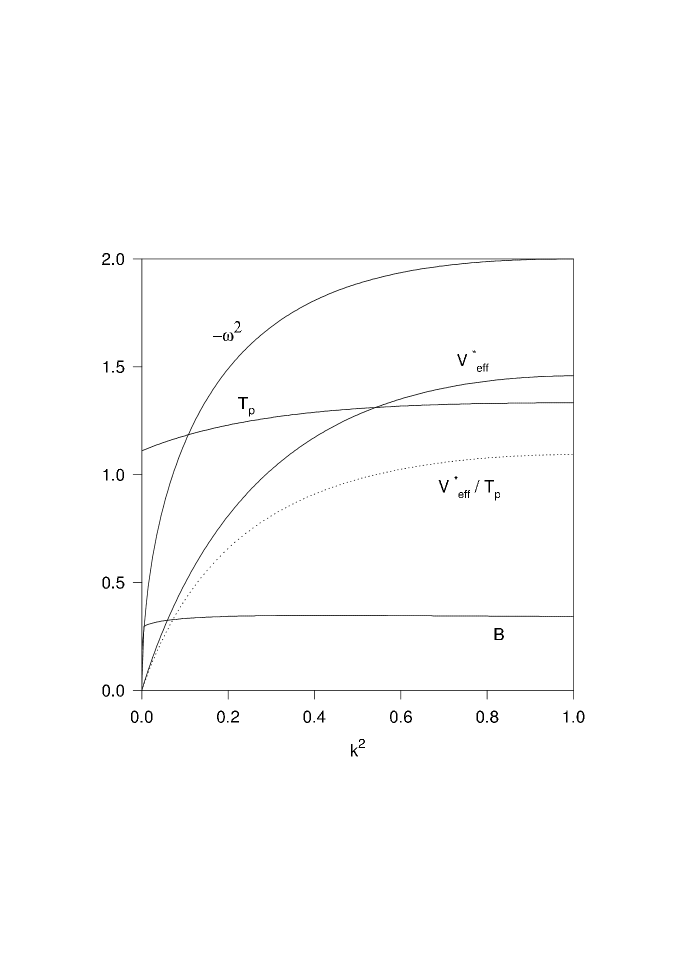
Figure 1: The brane tension $T_{p}$, the modulus of the potential value of the critical value $V_{eff}^{*}\equiv|V(\xi^{*})|$, the negative of the tachyonic eigenmode of the sphaleron $\omega^{2}\equiv\omega^{2}_{1}$ and the integral $B(k)$ are given as functions of $k^{2}$ for gauge- to Higgs boson mass $=\sqrt{2}$ ($N=1$). The ratio $V_{eff}^{*}/T_{p}$ is also shown.

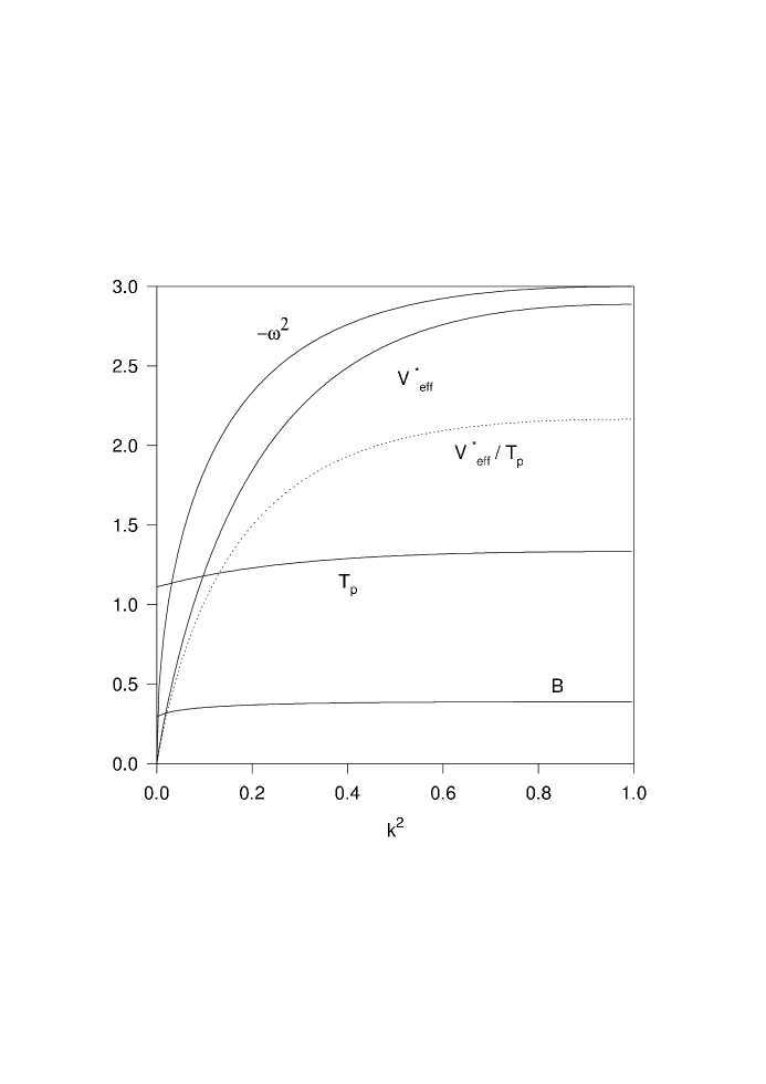
Figure 2: Same as Fig.1 for gauge- to Higgs boson mass $=\sqrt{2/3}$ ($N=2$).

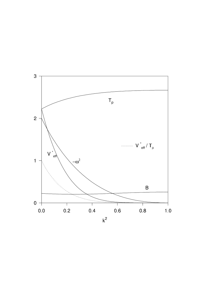
Figure 3: Same as Fig.1 for the model involving the $\phi^{4}$ scalar model of [9].

References

- [1] M. B. Green, Phys. Lett. B 329 (1994) 435; T. Banks and L. Susskind, Brane - Anti-Brane forces, hep-th/9511194; M. B. Green and M. Gutperle, Nucl. Phys. B 476 (1996) 484; G. Lifschytz, Phys. Lett. B 388 (1996) 720.
- [2] A. Sen, JHEP 9810 (1998), 021; JHEP 9812 (1998), 021; O. Bergman and M. R. Gaberdiel, Phys. Lett. B 441 (1998), 133; E. Witten, JHEP 9812 (1998), 019; P. Horava, Adv. Theor. Math. Phys. 2 (1999), 1373; J. A. Harvey, P. Horava and P. Kraus, JHEP 0003 (2000), 021.
- [3] A. Sen, Int. J. Mod. Phys. A 14 (1999) 4061; JHEP 08 (1998) 010; JHEP 08 (1998) 012; JHEP 09 (1998) 023.
- [4] E. Witten, Nucl. Phys. B 268 (1986) 253.
- [5] W. Taylor, Nucl. Phys. B 585 (2000) 171; N. Moeller and W. Taylor, Nucl. Phys. B 583 (2000) 105; R. de Mello Koch, A. Jevicki, M. Mihailescu and R. Tatar, Phys. Lett. B 482 (2000) 249; N. Moeller, A. Sen and B. Zwiebach, JHEP 08 (2000) 039; R. de Mello Koch and J. P. Rodrigues, Phys. Lett. B 495 (2000) 237; N. Moeller, hep-th/0008101; N. Berkovits, JHEP 04 (2000) 022; P. De Smet and J. Raeymaekers, JHEP 05 (2000) 051; A. Iqbal and N. Naqvi, hep-th/0004015; A. Sen and B. Zwiebach, JHEP 01 (2000) 009; W. Taylor, JHEP 08 (2000) 038; A. Iqbal and A. Naqvi, JHEP 01 (2001) 040; A. Sen, JHEP 12 (1999) 027; L. Rastelli and B. Zwiebach, JHEP 09 (2001) 038.
- [6] A. Sen and B. Zwiebach, JHEP 03 (2000) 002.
- [7] N. Berkovits, A. Sen and B. Zwiebach, Nucl. Phys. B 587 (2000) 147.
- [8] B. Zwiebach, JHEP 09 (2000) 028; J. A. Harvey and P. Kraus, JHEP 04 (2000) 012.
- [9] F. A. Brito, JHEP 08 (2005) 036.
- [10] A. V. Turbiner, Commun. Math. Phys. 118 (1988) 467.
- [11] Y. Brihaye, S. Giller, P. Kosinski and J. Kunz , Phys. Lett. B 293 (1992) 383.
- [12] L. Carson, Phys. Rev. D 42 (1990) 2853.
- [13] F. R. Klinkhamer and N. S. Manton, Phys. Rev. D 30 (1994) 2212.
- [14] Y. Brihaye and S. Braibant, J. Math. Phys. 34 (1993) 2107.