High-energy effective theory for a bulk brane

Abstract

We derive an effective theory describing the physics of a bulk brane in the context of the RS1 model. This theory goes beyond the usual low energy effective theory in that it describes the regime where the bulk brane has a large velocity and the radion can change rapidly. We achieve this by concentrating on the region where the distance between the orbifold planes is small in comparison to the AdS length scale. Consequently our effective theory will describe the physics shortly before a bulk/boundary or boundary/boundary brane collision. We study the cosmological solutions and find that, at large velocities, the bulk brane decouples from the matter on the boundary branes, a result which remains true for cosmological perturbations.

DAMTP-2005-90

I Introduction

The study of brane collisions has recently gained a special interest as it may provide a new scenario for the creation of the hot big-bang Universe CU ; Bubble . Motivated by heterotic M-theory and the Randall Sundrum (RS) model RSI , the collision between two orbifold branes has been explored, leading to a five-dimensional singularity Khoury:2001bz . When the boundary branes are close, an effective theory can be derived for this scenario and is hence valid just before or just after the collision collision ; CL ; CL2 ; CL3 ; CU . In this paper, we extend this analysis to the case where a brane is present in the bulk. This regime is of interest as it allows us to study a bulk/orbifold brane collision in a situation where the five-dimensional geometry remains regular similarly as in the first Ekpyrotic scenario CU . What is particularly interesting about the effective theory we will develop, is that it is capable of describing the regime where the branes have large velocities, something which the usual low energy effective theory cannot do.

Although similar work has been derived for close boundary branes, CL ; CL2 ; CL3 it relied strongly on the presence of a $\mathbb{Z}_{2}$ orbifold symmetry which is generically broken for bulk branes. This work will hence give us a general formalism for the derivation of an effective theory on a generic non $\mathbb{Z}_{2}$-brane. Such branes are interesting to study as they represent more realistic candidates for cosmology and at high-energies, their behaviour is expected to be strongly modified Davis:2000jq .

In order to get some insight on the brane geometry one should in principal solve the full higher-dimensional theory exactly before being able to infer the geometry on the brane. Unfortunately, this is only possible in very limited cases, and for more general situations, one should in practice either rely on numerical simulation or work in some specific regime where effective theories may be derived. This is the approach which is generally undertaken in order to derive a low-energy effective theory. Assuming a low-energy regime, it is possible to express the geometry on the brane as the lowest order of a gradient expansion CU ; GE ; Cotta ; Moduli . In this paper, we use a similar method, but choose instead to work in a close-brane regime, where we only consider terms of leading order in the distance between the branes. This method allow us to highlight the presence of “asymmetric” terms on the bulk brane (generic to the absence of $\mathbb{Z}_{2}$-symmetry) which are negligible at low-energies and are usually discarded. As far as we are aware, this is the first effective-theory that models these terms in a covariant way beyond the low-energy limit.
The rest of this paper is organized as follows. In Sec. II, we consider three branes and derive the effective theory on the asymmetric bulk brane. In that theory, two scalar dynamical degrees of freedom are present, namely the distance between the bulk brane and each of the boundary branes. We point out the low-energy limit of this theory, and check its consistency with previous results. In particular, we show that the theory on the bulk brane is a standard scalar-tensor theory of gravity coupled with two scalar fields. In Sec. III, we apply our effective theory to cosmology and compare our result with solutions from the five-dimensional theory. We show that for large velocities, the matter on the orbifold branes do not affect the bulk brane. As a specific example, we present the derivation of tensor perturbations. As expected, at large velocities the perturbations on the bulk brane decouple from the stress energy on the boundary branes. Finally, we summarize our study and present some possible extensions as future works in Sec. IV.

II Effective theory for Three close branes

Motivated by M-theory and the Randall-Sundrum model RSI , we consider spacetime to be effectively five-dimensional with the extra-dimension compactified on an $S^{1}/\mathbb{Z}_{2}$-orbifold. Two orbifold branes are located at the fixed point of the symmetry, and we consider a third brane in the bulk. In this paper, we shall be interested in the limit where the three branes are close to each other, i.e., when they are either about to collide or have just emerged from such a collision. In this paper we use the index conventions that Greek indices $\mu,\nu=0,\cdots,3$ are four dimensional, labeling the transverse $x^{\mu}$ directions, while Roman capital indices $M,N=0,\cdots,4$ are fully five dimensional and lower cap Roman indices $i,j=1,2,3$ designate the spatial transverse directions. Without loss of generality, we use the following metric ansatz

$$ds^{2}=g_{MN}dx^{M}dx^{N}=e^{2\varphi_{\pm}(y,x)}dy^{2}+g_{\mu\nu}(y,x)dx^{\mu}dx^{\nu}$$ (1)

and we suppose that the branes are located at $y=y_{+},y_{0},y_{-}$. The branes located at $y=y_{\pm}$ are the orbifold branes and they are subject to a $\mathbb{Z}_{2}$-reflection symmetry. The brane at $y=y_{+}$ is a positive tension brane, whereas the one at $y=y_{-}$ has a negative tension. The brane located at $y=y_{0}$ is a bulk brane and no symmetry is imposed.

In what follows, we denote by $\mathcal{R}_{+}$ (resp. $\mathcal{R}_{-}$) the region between the bulk brane and the positive (resp. negative) boundary brane. All through this paper we use the notation that an index ${}^{\prime}+^{\prime}$ (resp. ${}^{\prime}-^{\prime}$) represents a quantity evaluated in the region $\mathcal{R}_{+}$ (resp. $\mathcal{R}_{-}$), as shown in Fig. 1.

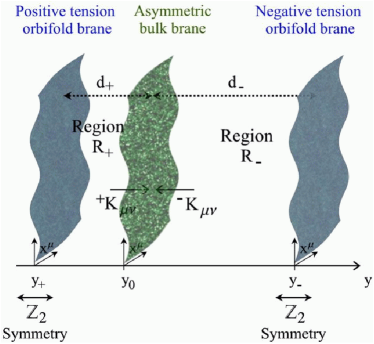
Figure 1: Two-brane Randall-Sundrum model with an asymmetric brane present in the bulk.

In particular, the Anti-de Sitter(AdS) length scale on each region will be denoted as $\ell_{\pm}$ and for any quantity $Q$, ${}^{\pm}Q(y_{0})=\lim_{\epsilon\rightarrow 0}Q(y_{0}\mp\epsilon)$. We denote by ${}^{(i)}T^{\mu}_{\nu}$ the stress-energy tensor for matter fields confined on the brane at $y=y_{i}$, for $i=+,-,0$. We assume all branes to have a tension $\sigma_{i}$ fine-tuned to their canonical value and absorb any departure in their stress-energy: $\sigma_{\pm}=\pm 6/\kappa^{2}\ell_{\pm}$ and $\sigma_{0}=3\left(\ell_{-}^{-1}-\ell_{+}^{-1}\right)/\kappa^{2}$ where $\kappa^{2}/8\pi$ is the five-dimensional gravitational constant.

The aim of this work is to derive an effective theory for the asymmetric bulk brane. We will hence work on the bulk brane frame throughout this paper unless otherwise specified. We will first decompose the extrinsic curvature on the bulk brane, in terms of a quantity that may be determined from the Israël matching condition and another “asymmetric” quantity which needs to be determined by other means. Working in the close-brane limit, we may express this “asymmetric” term as an expansion in terms of the extrinsic curvature on the orbifold branes which are uniquely determined by the junction conditions. The rest follows as in CL2 ; CL3 . In particular, we use the close-brane approximation to express the derivative of the extrinsic curvature in terms of the extrinsic curvature on the bulk brane as well as the one on the orbifold brane. This allows us to specify all unknown quantities in the modified Einstein equation of the bulk brane and hence obtain an effective theory for this brane.

II.1 Expression of the “asymmetric” term

For the boundary branes, the junction conditions are simply

$$K^{\mu}_{\nu}(y=y_{\pm})=-\frac{1}{\ell_{\pm}}\delta^{\mu}_{\nu}\mp\frac{\kappa^{2}}{2}\Bigl{(}{}^{(\pm)}T^{\mu}_{\nu}-\frac{1}{3}\delta^{\mu}_{\nu}{}^{(\pm)}T\Bigr{)},$$ (2)

where $K^{\mu}_{\nu}$ is the extrinsic curvature. Whereas for the bulk brane, due to the absence of any $\mathbb{Z}_{2}$-reflection symmetry, the extrinsic curvature cannot be uniquely determined by the junction conditions

$$\Delta K^{\mu}_{\nu}(y_{0}) := {}^{-}K^{\mu}_{\nu}(y_{0})-{}^{+}K^{\mu}_{\nu}(y_{0})$$ (3)

$$= \left(\frac{1}{\ell_{+}}-\frac{1}{\ell_{-}}\right)\delta^{\mu}_{\nu}-\kappa^{2}\Bigl{(}{}^{(0)}T^{\mu}_{\nu}-\frac{1}{3}\delta^{\mu}_{\nu}{}^{(0)}T\Bigr{)}.\hskip 10.0pt$$

Since we are interested in the close-brane limit, we assume in what follows, that the proper distance between the branes is much shorter than the AdS curvature scale. In this case, the following recursive relation is valid CL2 ; CL3 :

$${}^{\pm}K^{\mu(n)}_{\nu}(y_{0})=\hat{O}_{\pm}K^{\mu(n-2)}_{\nu}(y_{0})(y_{\pm}-y_{0})^{-2},$$ (4)

where ${}^{\pm}K^{\mu(n)}_{\nu}(y_{0})\equiv\partial_{y}^{\,n}\,{}^{\pm}\!K^{\mu}_{\nu}(y_{0})$ and the action of the operator $\hat{O}_{\pm}$ is defined by

$$\hat{O}_{\pm}S^{\mu}_{\nu}=D^{\mu}d_{\pm}D_{\alpha}d_{\pm}S^{\alpha}_{\nu}+D_{\nu}d_{\pm}D^{\alpha}d_{\pm}S^{\mu}_{\alpha}-(Dd_{\pm})^{2}S^{\mu}_{\nu}\hskip 5.0pt$$ (5)

for any symmetric tensor $S_{\mu\nu}=S_{(\mu\nu)}$. The proper distance between the branes is

$$d_{\pm}:=\pm e^{\varphi_{\pm}(y_{0},x)}(y_{0}-y_{\pm}),$$ (6)

in the gauge where $\varphi$ is independent of $y$. In Ref. CL2 , it is shown that the result is independent of this gauge choice.

Working in such a gauge, and using the five-dimensional Einstein equations, the Gauss equation on the brane is (Cf. Ref. SMS ),

$${}^{\pm}R^{\mu}_{\nu}(y_{0})=-\frac{4}{\ell_{\pm}^{2}}\delta^{\mu}_{\nu}+{}^{\pm}K(y_{0}){}^{\pm}K^{\mu}_{\nu}(y_{0})\\ +e^{-\varphi_{\pm}}{}^{\pm}K^{\prime\mu}_{\ \nu}(y_{0})+d_{\pm}^{-1}D^{\mu}D_{\nu}d_{\pm}.$$ (7)

The remaining task for the derivation of the effective theory is the evaluation of both ${}^{\pm}K^{\mu}_{\nu}(y_{0})$ and ${}^{\pm}K^{\prime\mu}_{\ \nu}(y_{0})$. We hence decompose ${}^{\pm}K^{\mu}_{\nu}(y_{0})$ into a “known” contribution $\Delta K^{\mu}_{\nu}$, and an undetermined part which represents the asymmetry across the brane:

$${}^{\pm}K^{\mu}_{\nu}(y_{0})=\mp\frac{1}{2}\Delta K^{\mu}_{\nu}(y_{0})+\bar{K}^{\mu}_{\nu}(y_{0}),$$ (8)

where $\bar{K}^{\mu}_{\nu}(y_{0}):=\frac{1}{2}\left({}^{+}K^{\mu}_{\nu}(y_{0})+{}^{-}K^{\mu}_{\nu}(y_{0})\right)$ and where the Codacci equation holds for both quantities independently: $D_{\mu}\left(\Delta K^{\mu}_{\nu}-\Delta K\delta^{\mu}_{\nu}\right)=D_{\mu}\left(\bar{K}^{\mu}_{\nu}-\bar{K}\delta^{\mu}_{\nu}\right)=0$. For a $\mathbb{Z}_{2}$-symmetric brane, $\bar{K}^{\mu}_{\nu}=0$.

Writing the extrinsic curvature on the orbifold branes as a Taylor expansion in terms of the one on the bulk brane, we have:

$$K^{\mu}_{\nu}(y_{\pm}) = \sum_{n\geq 0}^{\infty}\frac{1}{n!}{}^{\pm}K^{\mu(n)}_{\nu}(y_{0})(y_{\pm}-y_{0})^{n}$$

$$= \frac{{\rm sinh}{\sqrt{\hat{O}}_{\pm}}}{{\sqrt{\hat{O}}_{\pm}}}{}^{\pm}K^{\prime\mu}_{\ \nu}(y_{0})(y_{\pm}-y_{0})$$

$$+{\rm cosh}{\sqrt{\hat{O}}_{\pm}}{}^{\pm}K^{\mu}_{\nu}(y_{0}).$$

This provides an expression for the derivative of the extrinsic curvature

$${}^{\pm}K^{\prime\mu}_{\ \nu}(y_{0})=\frac{1}{y_{\pm}-y_{0}}\frac{{\sqrt{\hat{O}_{\pm}}}}{{\rm sinh}{\sqrt{\hat{O}_{\pm}}}}\Biggl{(}K^{\mu}_{\nu}(y_{\pm})\\ -{\rm cosh}{\sqrt{\hat{O}_{\pm}}}{}^{\pm}K^{\mu}_{\nu}(y_{0})\Biggr{)}.$$ (10)

Substituting this expression into Eq. (7) and recalling that the metric should be continuous across the bulk brane, ie. ${}^{+}R^{\mu}_{\nu}(y_{0})-{}^{-}R^{\mu}_{\nu}(y_{0})=0$, we obtain the constraint

$$\sum_{i=\pm}-\frac{i}{d_{i}}D^{\mu}D_{\nu}d_{i}+\frac{4i}{\ell_{i}^{2}}\delta^{\mu}_{\nu}-i\ {}^{i}\!K(y_{0})\,{}^{i}\!K^{\mu}_{\nu}(y_{0})$$ (11)

$$+\frac{1}{d_{i}}\frac{{\sqrt{\hat{O}_{i}}}}{{\rm sinh}{\sqrt{\hat{O}_{i}}}}\Biggl{(}K^{\mu}_{\nu}(y_{i})-{\rm cosh}{\sqrt{\hat{O}_{i}}}\ {}^{i}K^{\mu}_{\nu}(y_{0})\Biggr{)}=0.$$

Since the last two terms of the first line are of order $d^{0}$ and are hence negligible compared to the other ones which are of order $d^{-1}$, we can solve the above equation for the unknown part of ${}^{\pm}K^{\mu}_{\nu}(y_{0})$:

$$\bar{K}^{\mu}_{\nu}(y_{0})=\hat{L}\ Z^{\mu}_{\nu},$$ (12)

where the operator $\hat{L}$ is

$$\hat{L}=-\left[\frac{1}{d_{-}}\frac{{\sqrt{\hat{O}_{-}}}}{{\rm tanh}{\sqrt{\hat{O}_{-}}}}+\frac{1}{d_{+}}\frac{{\sqrt{\hat{O}_{+}}}}{{\rm tanh}{\sqrt{\hat{O}_{+}}}}\right]^{-1}$$ (13)

and

$$Z^{\mu}_{\nu}:=\sum_{i=\pm}\frac{i}{d_{i}}D^{\mu}D_{\nu}d_{i}-\frac{1}{d_{i}}\frac{\sqrt{\hat{O}_{i}}}{\sinh\sqrt{\hat{O}_{i}}}\ K^{\mu}_{\nu}(y_{i})\\ -\frac{i}{2d_{i}}\frac{\sqrt{\hat{O}_{i}}}{\tanh\sqrt{\hat{O}_{i}}}\ \Delta K^{\mu}_{\nu}(y_{0}).$$ (14)

It is worth pointing out that if a reflection symmetry was imposed across the bulk brane, we would have $d_{+}=d_{-}$, $\hat{O}_{+}=\hat{O}_{-}$ and $K^{\mu}_{\nu}(y_{+})=-K^{\mu}_{\nu}(y_{-})$. The tensor $Z^{\mu}_{\nu}$ would hence vanish, and so would $\bar{K}^{\mu}_{\nu}$.

II.2 Effective-theory

In the previous subsection, we have derived an expression for the “asymmetric” part of the extrinsic curvature in terms of quantities that can be determined from the Israël matching conditions and in terms of the first derivative of the extrinsic curvature. As far as we are aware this is the first derivation of the “asymmetric” term beyond the low-energy regime. Knowing the extrinsic curvature on the brane, we may use its expression in the Taylor expansion (II.1), to get an expression for the derivative (10) which can finally be substituted into the modified Einstein equation (7).

But first, we may express the equation of motion for the radions, which can be derived from the traceless property of the Weyl tensor ${}^{\pm}E^{\mu}_{\nu}(y_{0})$. Using the result of Ref. CL ; SMS , the Weyl tensor can be formally expressed as

$${}^{\pm}E^{\mu}_{\nu}(y_{0})=-e^{-\varphi_{\pm}}{}^{\pm}K^{\prime\mu}_{\ \nu}(y_{0})-\frac{1}{d_{\pm}}D^{\mu}D_{\nu}d_{\pm},$$ (15)

to leading order in $d_{\pm}$. Since $E^{\mu}_{\mu}(y_{0})=0$, this leads to the following Klein Gordon equation for the distance between the branes:

$$D^{2}d_{\pm}=\pm\,\delta^{\nu}_{\mu}\frac{\sqrt{\hat{O}_{\pm}}}{\sinh\sqrt{\hat{O}_{\pm}}}\Biggl{[}K^{\mu}_{\nu}(y_{\pm})-\cosh\sqrt{\hat{O}_{\pm}}\,{}^{\pm}\!K^{\mu}_{\nu}(y_{0})\Biggr{]},$$ (16)

where the right-hand side can be computed from Eqs. (8) and (12).

The tracelessness of the Weyl tensor together with the continuity constraint of the Ricci scalar across the brane, also implies the supplementary constraint on the asymmetric term $\bar{K}^{\mu}_{\nu}$:

$$\Delta K\bar{K}-\Delta K^{\alpha}_{\beta}\bar{K}^{\beta}_{\alpha}=6\left(\frac{1}{\ell_{-}^{2}}-\frac{1}{\ell_{+}^{2}}\right).$$ (17)

The formal expression for the Ricci scalar on the bulk brane is therefore:

$${}^{(4)}R = -6\left(\frac{1}{\ell_{+}^{2}}+\frac{1}{\ell_{-}^{2}}\right)+\bar{K}^{2}-\bar{K}^{\alpha}_{\beta}\bar{K}^{\beta}_{\alpha}$$

$$+\frac{1}{4}\Delta K^{2}-\frac{1}{4}\Delta K^{\alpha}_{\beta}\Delta K^{\beta}_{\alpha}.$$

We may now express the effective gravitational equation on the bulk brane. As expected, it can be described by two scalar fields non-trivially coupled to gravity:

$${}^{(4)}G^{\mu}_{\nu}(y_{0})=\frac{1}{d_{\pm}}(D^{\mu}D_{\nu}d_{\pm}-\delta^{\mu}_{\nu}D^{2}d_{\pm})\\ \mp\frac{1}{d_{\pm}}\left(\delta^{\mu}_{\beta}\delta^{\alpha}_{\nu}-\delta^{\mu}_{\nu}\delta^{\alpha}_{\beta}\right)\frac{{\sqrt{\hat{O}_{\pm}}}}{{\rm sinh}{\sqrt{\hat{O}_{\pm}}}}\\ \times\Biggl{[}K^{\beta}_{\alpha}(y_{\pm})-{\rm cosh}{\sqrt{\hat{O}_{\pm}}}{}^{\pm}K^{\beta}_{\alpha}(y_{0})\Biggr{]}.$$ (19)

The following formulae will be useful to rewrite the above equation in a more convenient way

$$\hat{O}\delta^{\mu}_{\nu}=2D^{\mu}dD_{\nu}d-\delta^{\mu}_{\nu}(Dd)^{2}$$ (20)

$$\hat{O}^{2}\delta^{\mu}_{\nu}=(Dd)^{4}\delta^{\mu}_{\nu}$$ (21)

$${\hat{O}}^{2}S^{\mu}_{\nu}=2D^{\mu}dD_{\nu}dD^{\alpha}dD_{\beta}dS^{\beta}_{\alpha}-(Dd)^{2}\hat{O}S^{\mu}_{\nu}$$ (22)

$${\hat{O}}^{2n}S^{\mu}_{\nu}=(Dd)^{4(n-1)}\hat{O}^{2}S^{\mu}_{\nu}~{}~{}(n\geq 1)$$ (23)

$${\hat{O}}^{2n+1}S^{\mu}_{\nu}=(Dd)^{4n}\hat{O}S^{\mu}_{\nu}$$ (24)

$${\rm cosh}{\sqrt{\hat{O}}}S^{\mu}_{\nu}=S^{\mu}_{\nu}+\frac{{\rm cos}|Dd|-1}{|Dd|^{2}}\hat{O}S^{\mu}_{\nu}+\frac{{\rm cosh}|Dd|+{\rm cos}|Dd|-2}{|Dd|^{4}}D^{\mu}dD_{\nu}dD_{\alpha}dD^{\beta}dS^{\alpha}_{\beta}$$ (25)

$$\frac{{\sqrt{\hat{O}}}}{{\rm sinh}{\sqrt{\hat{O}}}}S^{\mu}_{\nu}=S^{\mu}_{\nu}+\Biggl{(}\frac{|Dd|}{{\rm sin}|Dd|}-1\Biggr{)}|Dd|^{-2}\hat{O}S^{\mu}_{\nu}+\Biggl{(}\frac{|Dd|}{{\rm sin}|Dd|}+\frac{|Dd|}{{\rm sinh}|Dd|}-2\Biggr{)}|Dd|^{-4}D^{\mu}dD_{\nu}dD_{\alpha}dD^{\beta}dS^{\alpha}_{\beta}$$ (26)

$$\frac{{\sqrt{\hat{O}}}}{{\rm tanh}{\sqrt{\hat{O}}}}S^{\mu}_{\nu}=S^{\mu}_{\nu}+\Biggl{(}\frac{|Dd|}{{\rm tan}|Dd|}-1\Biggr{)}|Dd|^{-2}\hat{O}S^{\mu}_{\nu}+\Biggl{(}\frac{|Dd|}{{\rm tan}|Dd|}+\frac{|Dd|}{{\rm tanh}|Dd|}-2\Biggr{)}|Dd|^{-4}D^{\mu}dD_{\nu}dD_{\alpha}dD^{\beta}dS^{\alpha}_{\beta}.$$ (27)

II.3 Low-energy limit

In the slow-velocity limit, the effective theory simplifies greatly. We neglect the coupling of the radions to matter and neglect any terms beyond second order in derivatives. In that case, the expression for the asymmetric tensor $\bar{K}^{\mu}_{\nu}$ takes the form

$$\bar{K}^{\mu}_{\nu}(y_{0})=-\frac{1}{d}\left[d_{-}D^{\mu}D_{\nu}d_{+}-d_{+}D^{\mu}D_{\nu}d_{-}\right]$$ (28)

$$-\frac{\kappa^{2}}{2d}\left[d_{-}{}^{(+)}\tilde{T}^{\mu}_{\nu}-d_{+}{}^{(-)}\tilde{T}^{\mu}_{\nu}+\left(d_{-}-d_{+}\right){}^{(0)}\tilde{T}^{\mu}_{\nu}\right]$$

$$+\frac{1}{2\ell_{+}\ell_{-}}\left[-\left(\ell_{-}+\ell_{+}\right)+\frac{1}{d}\left(\ell_{+}d_{+}\hat{O}_{-}+\ell_{-}d_{-}\hat{O}_{+}\right)\right]\delta^{\mu}_{\nu},$$

where $d:=d_{+}+d_{-}$ and $\tilde{T}^{\mu}_{\nu}=T^{\mu}_{\nu}-\frac{1}{3}T\delta^{\mu}_{\nu}$. Using this expression in the modified Einstein equation (19), we obtain the induced Einstein tensor on the brane:

$${}^{(4)}G^{\mu}_{\nu}(y_{0})=\frac{1}{d}(D^{\mu}D_{\nu}d-\delta^{\mu}_{\nu}D^{2}d)+\frac{\kappa^{2}}{d}\ {}^{(\text{eff})}T^{\mu}_{\nu}\\ +\frac{1}{d}\Biggl{[}\frac{1}{\ell_{-}}D^{\mu}d_{-}D_{\nu}d_{-}+\frac{1}{2\ell_{-}}\left(Dd_{-}\right)^{2}\delta^{\mu}_{\nu}\\ -\frac{1}{\ell_{+}}D^{\mu}d_{+}D_{\nu}d_{+}-\frac{1}{2\ell_{+}}\left(Dd_{+}\right)^{2}\delta^{\mu}_{\nu}\Biggr{]},$$ (29)

where ${}^{(\text{eff})}T^{\mu}_{\nu}=(1/2){}^{(+)}T^{\mu}_{\nu}+(1/2){}^{(-)}T^{\mu}_{\nu}+{}^{(0)}T^{\mu}_{\nu}$. This is precisely the close-brane limit of the low-energy theory derived in Cotta , and is hence a good consistency check.

The equations of motion for the two scalar fields can be derived from Eqs. (16) and (17). Although Eq. (16) appears as two different equations, they are not independent and only give rise to the same following constraint for $D^{2}d$:

$$D^{2}d=\frac{\kappa^{2}}{3}\ {}^{(\text{eff})}T+\frac{1}{\ell_{-}}\left(Dd_{-}\right)^{2}-\frac{1}{\ell_{+}}\left(Dd_{+}\right)^{2}.$$ (30)

Using this result together with the continuity constraint (17), we obtain the decoupled Klein-Gordon equations for the two scalar fields at low-energy

$$D^{2}d_{\pm}=\frac{\kappa^{2}}{6}\left({}^{(\pm)}T\mp\frac{2\ell_{\pm}}{\ell_{-}-\ell_{+}}{}^{(0)}T\right)\mp\frac{1}{\ell_{\pm}}\left(Dd_{\pm}\right)^{2}.$$ (31)

As another check, we can verify that this result is consistent with the usual four-dimensional low-energy theory GE if a reflection symmetry was imposed across the brane. In that case $d_{+}=d_{-}$ and only one scalar field is coupled to gravity.

III Applications

In this section, we apply our effective theory to cosmology and perturbations. For the background solution, it is possible to solve the Einstein equation exactly. We may therefore use this feature to compare the exact five-dimensional result with our effective theory in the close-brane limit. This provides us a useful check. We will then use the effective theory in order to study cosmological perturbations around this background.

III.1 Cosmology

III.1.1 Five-dimensional solution

In this subsection, we first solve the five-dimensional Einstein equation exactly assuming cosmological symmetry (i.e. we assume the spacetime to be homogeneous and isotropic along the three spatial directions tangent to the branes). Working in the frame where the bulk is static, one may use the Birkhoff’s theorem to derive easily the exact form of the solution. But in order to compare this solution with our effective theory, it will be useful to work instead in the frame where the branes are static. Such a change of frame is in general difficult to perform, but working in the close-brane regime, and neglecting higher order terms in the distance between the branes, the change of frame may perform easily as it has been shown in Refs. CL2 ; CL3 . We will hence use the result of these papers to infer the geometry on the brane.

In the frame where the bulk is static, the geometry on both regions $\mathcal{R}_{\pm}$ is simply Schwarzschild-Anti-de Sitter (SAdS) with black-hole mass parameter $\mathcal{C}_{\pm}$:

$$ds^{2}_{\mathcal{R}_{\pm}} = -n_{\pm}^{2}dT_{\pm}^{2}+dY_{\pm}^{2}+a_{\pm}^{2}d\mathbf{x}^{2}$$ (32)

$$a_{\pm}^{2} = e^{-2Y_{\pm}/\ell_{\pm}}+\frac{\mathcal{C}_{\pm}}{4}e^{2Y_{\pm}/\ell_{\pm}}$$

$$n_{\pm}^{2} = a^{2}_{\pm}-\frac{\mathcal{C}_{\pm}}{a_{\pm}^{2}}.$$

It is important to notice that in this frame, the branes are not static, as in the previous section, and we will assume the branes to have loci $Y=Y_{i}(T)$. In particular, the bulk brane has loci $Y_{+}=Y_{0}^{(+)}(T_{+})$ with respect of the region $\mathcal{R}_{+}$, and loci $Y_{-}=Y_{0}^{(-)}(T_{-})$ as measured from an observed in the static bulk frame $\mathcal{R}_{-}$. The induced line element on the bulk brane can be read off as:

$$ds^{2}_{0} = -\left[n_{0}^{2}-\left(\frac{dY_{0}^{(\pm)}}{dT_{\pm}}\right)^{2}\right]dT_{\pm}^{2}+a_{0}^{2}\,d\mathbf{x}^{2}$$ (33)

$$= -dt^{2}+a_{0}^{2}\,d\mathbf{x}^{2},$$ (34)

where $a_{0}$ is the induced scale factor on the bulk brane: $a_{0}(t)=a_{+}\left(Y_{+}=Y_{0}^{(+)}(T_{+}(t))\right)=a_{-}\left(Y_{-}=Y_{0}^{(-)}(T_{-}(t))\right)$, and similarly for $n_{0}$. The physical time $t$ on the bulk brane, may be expressed in terms of the five-dimensional time coordinate $T_{\pm}$:

$$dt^{2}=\left[n_{0}^{2}-\left(\frac{dY_{0}^{(\pm)}}{dT_{\pm}}\right)^{2}\right]dT_{\pm}^{2}.$$ (35)

In order to derive the Friedmann equation on the branes, we may use the Israël junction conditions (3)

$$\Delta K^{i}_{j}(y_{0})=-\frac{\kappa^{2}}{3}\left(\sigma_{0}+\rho_{0}\right)\delta^{i}_{j},$$ (36)

where $\rho_{0}$ is the energy density of matter fields located on the brane and the extrinsic curvature is

$${}^{\pm}K^{i}_{j}(y_{0})=\delta^{i}_{j}\ \left(1-\frac{\dot{Y}_{0}^{(\pm)\,2}}{n_{0}^{2}}\right)^{-1/2}\left.\frac{da_{\pm}(Y)}{a_{\pm}dY_{\pm}}\right|_{Y_{0}^{(\pm)}},$$ (37)

where $\dot{Y}_{0}^{(\pm)}=dY_{0}^{(\pm)}(T_{\pm})/dT_{\pm}$. We may now re-express the extrinsic curvature in terms of the Hubble parameter on the brane. In particular we use the relation

$$\dot{Y}_{0}^{(\pm)}=\frac{da_{0}}{dt}\frac{dt}{dT_{\pm}}\left(\left.\frac{da_{\pm}(Y_{\pm})}{dY_{\pm}}\right|_{Y_{0}^{(\pm)}}\right)^{-1}.$$ (38)

Using the fact that $da_{\pm}/dY_{\pm}=-n_{\pm}/\ell_{\pm}$, we have:

$$\dot{Y}_{0}^{(\pm)\,2}=\frac{\ell_{\pm}^{2}a^{2}_{0}H^{2}}{1+\ell^{2}_{\pm}\,a_{0}^{2}\,H^{2}/n_{0}^{2}},$$ (39)

where $H$ is the Hubble parameter on the brane $H=(da_{0}/dt)/a_{0}$. The extrinsic curvature on each side of the bulk brane can therefore be expressed in terms of the Hubble parameter as:

$${}^{\pm}K^{i}_{j}(y_{0}) = -\delta^{i}_{j}\ \sqrt{\frac{n_{0}^{2}}{\ell_{\pm}^{2}a_{0}^{2}}+H^{2}},$$ (40)

$$= -\delta^{i}_{j}\ \sqrt{\frac{1}{\ell_{\pm}^{2}}-\frac{\mathcal{C}_{\pm}}{\ell_{\pm}^{2}a_{0}^{4}}+H^{2}}.$$

Having an expression for the extrinsic curvature in terms of the Hubble parameter on each side of the bulk brane, we can therefore use the Israël matching condition Eq. (36) to express the Hubble parameter on the brane in terms on the energy density and the black-hole mass parameters. Substituting Eq. (40) into (36), we find the modified Friedmann equation on the asymmetric bulk brane:

$$H^{2}=\frac{T_{b}^{2}}{4}+\frac{1}{4T_{b}^{2}}\left[\frac{1}{\ell_{+}^{2}}-\frac{1}{\ell_{-}^{2}}-\frac{1}{a_{0}^{4}}\left(\frac{\mathcal{C}_{+}}{\ell_{+}^{2}}-\frac{\mathcal{C}_{-}}{\ell_{-}^{2}}\right)\right]^{2}\\ -\frac{1}{2}\left[\frac{1}{\ell_{+}^{2}}+\frac{1}{\ell_{-}^{2}}-\frac{1}{a_{0}^{4}}\left(\frac{\mathcal{C}_{+}}{\ell_{+}^{2}}+\frac{\mathcal{C}_{-}}{\ell_{-}^{2}}\right)\right],$$ (41)

with $T_{b}=\frac{\kappa^{2}}{3}\left(\sigma_{0}+\rho_{0}\right)$. In this modified Friedmann equation, one might think that the parameters $\mathcal{C}_{\pm}$ are arbitrary, but in what follows, we show that they depend strongly on the brane velocities and find the precise relation between them. This is important as it will allow us to compare this result with the one obtained from the effective close-brane theory which gives a direct relation with the brane velocities.

III.1.2 Expression for the velocity of the branes.

Without loss of generality, we work in the specific situation where the bulk brane is about to collide with the positive boundary brane ($\dot{d}_{+}<0$), and moves away from the negative boundary brane ($\dot{d}_{-}>0$). The velocity of both boundary branes should therefore be positive while the velocity of the bulk brane should be negative. In the case where the bulk brane has a positive canonical tension, $\ell_{+}>\ell_{-}$ the Hubble constant on the bulk brane will be positive.

We may now use the results of Refs. CL2 ; CL3 where the the following relation for the radion velocity holds in the close-brane regime:

$$\dot{d}_{\pm}=\mp\left(\tanh^{-1}\left(\frac{v_{\pm}}{n_{0}}\right)+\tanh^{-1}\left(\frac{{}^{\pm}v_{0}}{n_{0}}\right)\right),$$ (42)

where $v_{\pm}$ are the absolute value of velocities of the boundary branes with respect to five-dimensional physical time at the collision and ${}^{\pm}v_{0}=\left|dY_{0}^{(\pm)}/dT_{\pm}\right|$ is the absolute value of the velocity of the bulk brane as measured by a static observer in region $\mathcal{R}_{\pm}$. In what follows, a dot designates the derivative with respect to the physical time $t$ on the bulk brane.

Using the result of Ref. CL3 , one has:

$$\left(\frac{v_{\pm}}{n_{0}}\right)=\sqrt{1-\frac{1-\mathcal{C}_{\pm}/a_{0}^{4}}{\left(1\pm\frac{1}{6}\kappa^{2}\ell_{\pm}\rho_{\pm}\right)^{2}}},$$ (43)

where $\rho_{\pm}$ is the energy density on the $\pm$-brane. Using the expression (39), one has the expression for the bulk brane velocity

$$\left(\frac{{}^{\pm}v_{0}}{n_{0}}\right)=\frac{\ell_{\pm}H}{\sqrt{\ell_{\pm}^{2}H^{2}+1-\mathcal{C}_{\pm}/a^{4}_{0}}}.$$ (44)

The radions’ velocities $\dot{d}_{\pm}$ can hence be expressed in terms of the black-hole mass parameter $\mathcal{C}_{\pm}$

$$\dot{d}_{\pm}=\mp\tanh^{-1}\sqrt{1-\frac{1-\mathcal{C}_{\pm}/a_{0}^{4}}{\left(1\pm\frac{1}{6}\kappa^{2}\ell_{\pm}\rho_{\pm}\right)^{2}}}\\ \mp\tanh^{-1}\left(\frac{\ell_{\pm}H}{\sqrt{\ell_{\pm}^{2}H^{2}+1-{\mathcal{C}_{\pm}}/{a_{0}^{4}}}}\right).$$ (45)

We may use these equations to find an expression for the constants $\mathcal{C}_{\pm}$ in terms of the brane velocities:

$$\frac{\mathcal{C}_{\pm}}{a_{0}^{4}}=\left[\frac{\pm\,\ell_{\pm}H+\sinh\dot{d}_{\pm}\left(1\pm\frac{1}{6}\kappa^{2}\ell_{\pm}\rho_{\pm}\right)}{\cosh\dot{d}_{\pm}}\right]^{2}\\ \mp\frac{1}{6}{\kappa^{2}\ell_{\pm}}\rho_{\pm}\left(2\pm\frac{1}{6}{\kappa^{2}\ell_{\pm}}\rho_{\pm}\right).$$ (46)

Using this relation for $\mathcal{C}_{-}$, one has

$$H^{2}+\frac{1-\mathcal{C}_{-}/a_{0}^{4}}{\ell_{-}^{2}}=\left(\frac{1-\frac{1}{6}{\kappa^{2}\ell_{-}}\rho_{-}+\ell_{-}H\sinh\dot{d}_{-}}{\ell_{-}\cosh\dot{d}_{-}}\right)^{2}.$$ (47)

But from Eq. (41), one has as well:

$$H^{2}+\frac{1-\mathcal{C}_{-}/a_{0}^{4}}{\ell_{-}^{2}}=\\ \left[\frac{T_{b}}{2}-\frac{1}{2T_{b}}\left(\frac{1}{\ell_{+}^{2}}-\frac{1}{\ell_{-}^{2}}+\frac{\mathcal{C}_{-}}{a_{0}^{4}\ell_{-}^{2}}-\frac{\mathcal{C}_{+}}{a_{0}^{4}\ell_{+}^{2}}\right)\right]^{2}.$$ (48)

Substituting the expression (46) for $\mathcal{C}_{\pm}$ into the last line, we therefore have an equation for $H$ in terms of $\dot{d}_{\pm}$, which has for solution:

$$H=\Lambda^{\text{eff}}+\frac{1}{6}{\alpha\kappa^{2}}\rho_{0}^{\text{eff}},$$ (49)

with the notation

$$\rho_{0}^{\text{eff}} =\frac{\rho_{-}}{2\cosh\dot{d}_{-}}+\frac{\rho_{+}}{2\cosh\dot{d}_{+}}+\rho_{0},$$

$$\Lambda^{\text{eff}} =\frac{\alpha}{2\ell_{-}}\left(1-\frac{1}{\cosh\dot{d}_{-}}\right)-\frac{\alpha}{2\ell_{+}}\left(1-\frac{1}{\cosh\dot{d}_{+}}\right),$$

$$\alpha =2\left(\tanh\dot{d}_{+}+\tanh\dot{d}_{-}\right)^{-1}.$$

We may now compare this result with what is obtained from the effective theory. But first, we might make some important remarks. At low-energy, the contribution from the matter on each brane has an equal weight: $\rho_{0}^{\text{eff}}\simeq\left(\rho_{-}/2+\rho_{+}/2+\rho_{0}\right)$. This is due to the fact, that at low-energy, when the branes are close, the bulk geometry is almost Minkowski and each brane has an equal contribution. This result is however not obvious from the usual Friedmann equation (41), where only the matter on the bulk brane seems to contribute, but one should take into account the expression of $\mathcal{C}_{\pm}$ in terms of $\rho_{\pm}$. However, at high-velocities, the situation is radically different: The geometry on the bulk brane decouples entirely from the matter content on the orbifold branes (we may point out that this result is valid for the two-brane case as well Cf. Ref. CL3 ). In that limit, we indeed have $\rho_{0}^{\text{eff}}\rightarrow\rho_{0}$, with an effective cosmological constant $({1}/{2})\left|{1}/{\ell_{+}}-{1}/{\ell_{-}}\right|$. Its contribution vanishes when the asymmetry across the brane is maximal: $\ell_{+}=\ell_{-}$. In that case the bulk geometry is almost unperturbed by the brane and the Friedmann equation on the bulk brane couples quadratically to its own matter $H^{2}_{0}={\kappa^{4}}\rho_{0}^{2}/36$. This is an exact result arising from the five-dimensional equations of motions in the close brane and high-velocity limit.

III.1.3 Cosmology in the effective theory

We now wish to compare this exact result with the predictions from the close-brane effective theory. The modified Einstein equation (19) on the bulk brane reads:

$$G^{i}_{j}(y_{0}) = \left(H^{2}-\frac{1}{3}R^{2}\right)\delta^{i}_{j}\sim d^{0}$$ (50)

$$= \frac{1}{d_{-}}D^{i}D_{j}d_{-}+\frac{(y_{-}-y_{0})}{d_{-}}\,{}^{-}K^{\prime\,i}_{\,\,j}\sim d^{-1}.\ \$$

Since the first line is of higher order in the distance between the brane, the second line should vanish. The expression for the derivative of the extrinsic curvature can be found in (10), and using the relation $\hat{O}_{\pm}Z^{i}_{j}=\dot{d}_{\pm}^{2}Z^{i}_{j}$ valid for the background, we therefore have the equation:

$$0=-H\dot{d}_{-}\delta^{i}_{j}+\frac{\dot{d}_{-}}{\sinh\dot{d}_{-}}K^{i}_{j}(y_{-})\\ -\frac{\dot{d}_{-}}{\tanh\dot{d}_{-}}\left(\frac{1}{2}\Delta K^{i}_{j}(y_{0})+\bar{K}^{i}_{j}(y_{0})\right),$$ (51)

where $\Delta K^{i}_{j}(y_{0})$ is given in Eq. (36),

$$K^{i}_{j}(y_{\pm})=\left(-\frac{1}{\ell_{\pm}}\mp\frac{\kappa^{2}}{6}\rho_{\pm}\right)\delta^{i}_{j},$$ (52)

and $\bar{K}^{i}_{j}$ is given by:

$$\bar{K}^{i}_{j} = -\Biggl{[}-\frac{\dot{d}_{-}}{d_{-}\sinh\dot{d}_{-}}K^{i}_{j}(y_{-})-\frac{\dot{d}_{+}}{d_{+}\sinh\dot{d}_{+}}K^{i}_{j}(y_{+})$$

$$+ \frac{1}{2}\left(\frac{\dot{d}_{-}}{d_{-}\tanh\dot{d}_{-}}-\frac{\dot{d}_{+}}{d_{+}\tanh\dot{d}_{+}}\right)\Delta K^{i}_{j}(y_{0})$$

$$+ H\left(\frac{\dot{d}_{-}}{d_{-}}-\frac{\dot{d}_{+}}{d_{+}}\right)\delta^{i}_{j}\Biggr{]}\left(\frac{\dot{d}_{+}}{d_{+}\tanh\dot{d}_{+}}+\frac{\dot{d}_{-}}{d_{-}\tanh\dot{d}_{-}}\right)^{-1}.$$

Using these expressions (36), (52) and (III.1.3) in the Eq. (51) for $H$, we finally obtain the relation between the Hubble parameter on the asymmetric brane and the radions’ velocities:

$$H=\Lambda^{\text{eff}}+\frac{1}{6}{\alpha\kappa^{2}}\rho_{0}^{\text{eff}},$$ (54)

with the same notations as for Eq. (49). This corresponds precisely to what was obtained from the exact five-dimensional theory and represents an important consistency check.

We may also wonder whether this theory is capable of reproducing the expression (41) for the Hubble parameter. This Friedmann equation is a simple consequence of the tracelessness of the Weyl tensor as we shall see. Using this property for the Weyl tensor, we have indeed obtained in Eq. (II.2) an expression for the Ricci scalar in terms of $\bar{K}^{\mu}_{\nu}$ and $\Delta K^{\mu}_{\nu}$. The expression of $\Delta K^{\mu}_{\nu}$ is in general complicated, but for cosmological solutions the Eq. (17) imposes the constraint:

$$\bar{K}^{0}_{0}=\left(-2-\frac{\Delta K^{0}_{0}}{\Delta K^{1}_{1}}\right)\bar{K}^{1}_{1}+\frac{2}{\Delta K^{1}_{1}}\left(\frac{1}{\ell_{+}^{2}}-\frac{1}{\ell_{-}^{2}}\right),$$ (55)

which we may reexpress as

$$\bar{K}^{0}_{0}=\frac{-\kappa^{2}p_{0}-3x}{x-\kappa^{2}\rho_{0}/3}\bar{K}^{1}_{1}-\frac{2xy}{x-\kappa^{2}\rho_{0}/3},$$ (56)

where for simplicity we wrote $x=\ell_{+}^{-1}-\ell_{-}^{-1}$ and $y=\ell_{+}^{-1}+\ell_{-}^{-1}$. Furthermore, from the Codacci equation, we have the relation

$$\partial_{a}\bar{K}^{1}_{1}(a)=a\left(\bar{K}^{0}_{0}-\bar{K}^{1}_{1}\right).$$ (57)

Using this result together with the conservation of energy condition $p_{0}=-a\rho_{0}^{\prime}(a)/3-\rho_{0}$, we may solve this differential equation for $\bar{K}^{1}_{1}$ and obtain

$$\bar{K}^{1}_{1}=-\frac{xy}{2\left(x-\kappa^{2}\rho_{0}/3\right)}+\frac{C_{\text{A}}}{a_{0}^{4}\left(x-\kappa^{2}\rho_{0}/3\right)},$$ (58)

where the “asymmetric” constant $C_{\text{A}}$ appears as an integration constant. We may now use this expression in Eq. (II.2):

$$R = 6aHH^{\prime}(a)+12H^{2}$$

$$= \left[-\frac{\left({2C_{\text{A}}}/{a^{4}}-xy\right)^{2}}{2T_{b}^{3}}+\frac{1}{2}T_{b}^{2}\right]a\,\rho^{\prime}_{0}(a)$$

$$+ \frac{1}{T_{b}^{2}}\left[-12\left(\frac{C_{\text{A}}}{a^{4}}\right)^{2}+\left(y^{2}-T_{b}^{2}\right)\left(x-T_{b}\right)\rho_{0}(a)\right],$$

where $T_{b}=T_{b}(a)=(1/3){\kappa^{2}}\left(\sigma_{0}+\rho_{0}(a)\right)$. This is simply a first order differential equation for $H(a)$, of which solution is

$$H^{2}=\frac{T_{b}^{2}}{4}+\frac{1}{4T_{b}^{2}}\left(-xy+2\frac{C_{\text{A}}}{a_{0}^{4}}\right)^{2}-\frac{1}{4}\left(x^{2}+y^{2}+\frac{C_{S}}{a_{0}^{4}}\right).$$ (60)

The parameter $C_{\text{S}}$ appears as an integration constant as well. This expression corresponds precisely to the Friedmann equation (41) obtained by solving the five-dimensional geometry, and we can now relate the black-hole mass parameters to the integration constants $C_{\text{A}}$ and $C_{\text{S}}$

$$C_{\text{A}} = \frac{1}{2}\left(\frac{\mathcal{C}_{+}}{\ell_{-}^{2}}-\frac{\mathcal{C}_{-}}{\ell_{+}^{2}}\right)$$ (61)

$$C_{S} = -2\left(\frac{\mathcal{C}_{+}}{\ell_{-}^{2}}+\frac{\mathcal{C}_{-}}{\ell_{+}^{2}}\right).$$ (62)

In particular, the contribution from $C_{\text{S}}$ should be expected in a general case and is responsible for the dark energy term. The contribution of $C_{\text{A}}$ is specific to the asymmetric brane and should cancel when $\bar{K}^{\mu}_{\nu}=0$, this is indeed the case when one has opposite AdS scales on each regions $\mathcal{R}_{\pm}$: $\ell_{-}=-\ell_{+}$, and when the black-hole mass parameters are the same: $\mathcal{C}_{-}=\mathcal{C}_{+}$. In a general case it is not possible to deduce the expression of the asymmetric term by solving the five-dimensional theory, and our theory provides a useful alternative. This is for instance the case for the study of perturbations.

III.2 Cosmological perturbations

The aim of this paper is to provide an effective theory capable of describing a bulk brane geometry in a consistent way, beyond the low-energy approximation. In this paper we will hence not extend this study to a large analysis of perturbations, which would be a subject on its own, but we may point out some useful comments which will be relevant for such a study. In particular, we have seen in the previous section, that at high-velocities, the geometry on the bulk brane decouples from the matter content of the orbifold branes. This result was valid for cosmology and we may check the effect of tensor perturbations.

First we may stress that the operators $\hat{O}_{+}$ and $\hat{O}_{-}$ do not commute in general. For a symmetric tensor $S_{\mu\nu}=S_{\left(\mu\nu\right)}$,

$$\left[\hat{O}_{-},\hat{O}_{+}\right]S^{\mu}_{\nu}=\Big{[}\left(D^{\mu}d_{-}D_{\beta}d_{+}-D^{\mu}d_{+}D_{\beta}d_{-}\right)S^{\beta}_{\nu}\\ +\left(D_{\nu}d_{-}D^{\beta}d_{+}-D_{\nu}d_{+}D^{\beta}d_{-}\right)S^{\mu}_{\beta}\Big{]}\left(D_{\alpha}d_{-}\,D^{\alpha}d_{+}\right).$$ (63)

So apart for cosmology and for tensor, vector perturbations or if we work in a gauge where both $\delta d_{-}$ and $\delta d_{+}$ may be set to zero, the order of the action of the different operators in the effective theory is important. In particular we expect this feature to have consequences on the evolution of non-linear perturbations.

As a specific simple example, one might study here the evolution of tensor perturbations:

$$ds^{2}_{0}=a^{2}\left[-d\tau^{2}+\left(\delta_{ij}+h_{ij}\right)dx^{i}dx^{j}\right],$$ (64)

where $\tau$ is the conformal time on the bulk brane and we write $h^{i}_{j}=\delta^{ik}h_{kj}$. For tensor perturbations, the right hand side of the modified Einstein equation (19) is hence:

$$\delta G^{i}_{j}=\delta R^{i}_{j}=-\frac{({\dot{d}_{+}}/{2d_{+}})X_{-}+({\dot{d}_{-}}/{2d_{-}})X_{+}}{X_{-}+X_{-}}\ \dot{h}^{i}_{j}\\ +\kappa^{2}\,\frac{X_{-}X_{+}}{X_{-}+X_{+}}\ {}^{(\text{eff})}\!\delta T^{i}_{j},$$ (65)

with the effective matter contribution:

$${}^{(\text{eff})}\!\delta T^{i}_{j}=\frac{1}{2\cosh\dot{d}_{-}}\,{}^{(-)}\!\delta T^{i}_{j}+\frac{1}{2\cosh\dot{d}_{+}}\,{}^{(+)}\!\delta T^{i}_{j}+\,{}^{(0)}\!\delta T^{i}_{j},$$ (66)

where ${}^{(k)}\!\delta T^{i}_{j}$ is the tensor part of matter perturbations on the brane at $y=y_{k}$. For simplicity, we wrote $X_{\pm}=\dot{d}_{\pm}/\left(d_{\pm}\tanh\dot{d}_{\pm}\right)$. The only non-negligible part in the perturbation of the Ricci tensor is $\delta R^{i}_{j}=-\frac{\bar{\partial^{2}}}{2a_{0}^{2}}\,h^{i}_{j}$, the evolution of the tensor perturbations, is hence controlled by

$$\hat{\boxdot}\,h^{i}_{j}=-a_{0}^{2}\,\Omega\kappa^{2}\ {}^{(\text{eff})}\!\delta T^{i}_{j},$$ (67)

with

$$\hat{\boxdot} =\left[\bar{\partial^{2}}-\frac{d^{\prime}_{+}d^{\prime}_{-}}{d_{+}d_{-}}\frac{\tanh\dot{d}_{+}+\tanh\dot{d}_{-}}{\frac{d^{\prime}_{+}}{d_{+}}\tanh\dot{d}_{+}+\frac{d^{\prime}_{-}}{d_{-}}\tanh\dot{d}_{-}}\partial_{\tau}\right],$$

$$\Omega =2\left(\frac{d_{+}\tanh\dot{d}_{+}}{\dot{d}_{+}}+\frac{d_{-}\tanh\dot{d}_{-}}{\dot{d}_{-}}\right)^{-1},$$

where a prime designates derivative with respect to the conformal time $\tau$ and the operator $\bar{\partial^{2}}$ is the Laplacian in Minkowski space. One may note that in the close brane limit, if $d_{\pm}\sim\dot{d}_{\pm}t$, the damping term $\frac{d^{\prime}_{+}d^{\prime}_{-}}{d_{+}d_{-}}\frac{\tanh\dot{d}_{+}+\tanh\dot{d}_{-}}{({d^{\prime}_{+}}/{d_{+}})\tanh\dot{d}_{+}+({d^{\prime}_{-}}/{d_{-}})\tanh\dot{d}_{-}}$ simply goes as $\tau^{-1}$, which is what is expected from a usual four-dimensional theory. The expression for the effective four-dimensional Newtonian constant is on the other hand slightly affected: $\kappa_{(4d)}^{2}=\kappa^{2}\Omega$, which is similar to the result obtained in Ref. CL3 . For more sophisticated analysis, we however expect the result to be more interesting, especially when the operators $\hat{O}_{\pm}$ do not commute.

However, we may point out that the remarks formulated for the background remain valid at the level of perturbations. Namely, for large brane velocities, the effective matter contribution on the bulk brane is

$${}^{(\text{eff})}\!\delta T^{i}_{j}\rightarrow\,{}^{(0)}\!\delta T^{i}_{j},$$ (68)

and perturbations are not sensitive to the matter content of the orbifold branes. This provides a braneworld scenario, where the branes could be close (and hence the Kaluza Klein modes difficult to excite and to affect the brane), and yet the geometry on the bulk brane would decouple from the other ones.

IV Summary and Discussion

In this paper, an effective theory describing the gravitational behaviour of a bulk brane has been derived. The absence of any reflection symmetry across a generic bulk brane makes its behaviour especially interesting to study. In the “light”-brane limit, ie. when the five-dimensional geometry is almost unaffected by the presence of the brane, the asymmetry on the brane itself is important and affects its own behaviour. In this work, we have developed a four-dimensional effective theory capable of describing this “asymmetry” in a covariant way. For that, we have considered a close-brane approximation, where we assumed the bulk brane to be close to both orbifold branes.

Using this approximation, we obtained a resulting theory of gravity coupled in a non-trivial way with two scalar fields representing the distance between the bulk brane and each of the orbifold branes. This four-dimensional theory can be tested in several limits, such as at low-energy, when a reflection symmetry is imposed by hand and for cosmology. In all these regimes, predictions from the close-brane theory agree perfectly with the expected results. The case of cosmology is of special interest, at high-velocity the bulk geometry is not sensitive to the matter present on the orbifold branes, and this result remains valid for tensor perturbations. In the limit where the AdS length scale is the same on both side of the brane, ie. the bulk is not perturbed by the brane, we show that the Hubble parameter couples linearly to the energy density on the bulk brane. This is an interesting result, which might strongly affect the gravitational behaviour on such a brane.

This effective theory could as well be derived on the orbifold branes in the presence of such a brane in the bulk. We may point out that the asymmetric tensor we derived on the bulk brane depends on the bulk brane metric. It will hence be necessary to find its expression in terms of the orbifold brane metric before being able to derive an effective theory for these orbifold branes. This is left for a future study.

A straightforward extension of this model, would be the scenario where the bulk brane is close to only one of the orbifold branes, and the radion representing the distance with the other orbifold brane is moving slowly. One side of the theory would hence be modeled by the low-energy effective theory while the close-brane theory would be a good description for the other side. Such a model would be of interest if one considers the collision of the bulk brane with one of the orbifold branes. Such a process might produce a phase transition which could have some interesting consequences from a cosmological point of view. This is also left for a future study.

References

• (1) J. Khoury, B. A. Ovrut, P. J. Steinhardt and N. Turok, Phys. Rev. D64, 123522(2001).
• (2) U. Gen, A. Ishibashi and T. Tanaka Phys. Rev. D66, 023519(2002); J. J. Blanco-Pillado, M. Bucher, S. Ghassemi and F. Glanois, Phys. Rev. D69, 103515(2004).
• (3) L. Randall and R. Sundrum, Phys. Rev. Lett. 83, 3370 (1999).
• (4) J. Khoury, B. A. Ovrut, N. Seiberg, P. J. Steinhardt and N. Turok, Phys. Rev. D 65, 086007 (2002) [arXiv:hep-th/0108187].
• (5) A. Neronov, JHEP 0111, 007(2001); D. Langlois, K. Maeda and D. Wands, Phys. Rev. Lett. 88, 181301(2002); S. Kanno, M. Sasaki and J. Soda, Prog. Theor. Phys. 109, 357(2003).
• (6) T. Shiromizu, K. Koyama and K. Takahashi, Phys. Rev. D67, 104011(2003).
• (7) C. de Rham and S. Webster, Phys. Rev. D71, 124025(2005).
• (8) C. de Rham and S. Webster, Phys. Rev. D72, 64013(2005).
• (9) A. C. Davis, S. C. Davis, W. B. Perkins and I. R. Vernon, Phys. Lett. B504, 254(2001); B. Carter and J. P. Uzan, Nucl. Phys. B606, 45(2001); K. Takahashi and T. Shiromizu, Phys. Rev. D70, 103507(2004); L. A. Gergely, E. Leeper and R. Maartens, Phys. Rev. D70, 104025(2004); I. R. Vernon and D. Jennings, JCAP 0507, 011(2005).
• (10) T. Wiseman, Class. Quant. Grav. 19, 3083(2002); S. Kanno and J. Soda, Phys. Rev. D66, 043526(2002); ibid, 083506,(2002); T. Shiromizu and K. Koyama, Phys. Rev. D67, 084022(2003); C. de Rham, Phys. Rev. D71, 024015(2005).
• (11) L. Cotta-Ramusino, “Low energy effective theory for brane world models”, MPhill. thesis, University of Portsmouth(2004).
• (12) J. Garriga, O. Pujolas and T. Tanaka, Nucl. Phys. B655, 127(2003); P. Brax, C. van de Bruck, A. C. Davis and C. S. Rhodes, Phys. Rev. D67, 023512(2003); G. A. Palma and A. C. Davis, Phys. Rev. D70, 106003(2004); S. L. Webster and A. C. Davis, hep-th/0410042; S. Kanno and J. Soda, Phys.Rev. D71, 044031(2005).
• (13) T. Shiromizu, K. Maeda and M. Sasaki, Phys. Rev. D62, 024012(2000).