Effective Action and Phase Structure
of Multi–Layer Sine–Gordon Type Models

Abstract

We analyze the effective action and the phase structure of $N$-layer sine-Gordon type models, generalizing the results obtained for the two-layer sine-Gordon model found in [I. Nándori, S. Nagy, K. Sailer and U. D. Jentschura, Nucl. Phys. B 725, 467–492 (2005)]. Besides the obvious field theoretical interest, the layered sine-Gordon model has been used to describe the vortex properties of high transition temperature superconductors, and the extension of the previous analysis to a general $N$-layer model is necessary for a description of the critical behaviour of vortices in realistic multi-layer systems. The distinction of the Lagrangians in terms of mass eigenvalues is found to be the decisive parameter with respect to the phase structure of the $N$-layer models, with neighbouring layers being coupled by quadratic terms in the field variables. By a suitable rotation of the field variables, we identify the periodic modes (without explicit mass terms) in the $N$-layer structure, calculate the effective action and determine their Kosterlitz–Thouless type phase transitions to occur at a coupling parameter $\beta^{2}_{{\rm c},N}=8N\pi$, where $N$ is the number of layers (or flavours in terms of the multi-flavour Schwinger model).

1 Introduction

The phase structure of generalized sine-Gordon (SG) type models is known to crucially depend on the periodicity of the interaction Lagrangian in the field variable. The “pure” SG model is periodic in the internal space spanned by the field variable. The double-layer sine-Gordon (LSG) model [1, 2] is characterized by the Lagrangian

$${\mathcal{L}}_{\rm 2LSG}={\frac{1}{2}}\,(\partial\varphi_{1})^{2}+{\frac{1}{2}}\,(\partial\varphi_{2})^{2}+{1\over 2}\,J(\varphi_{1}-\varphi_{2})^{2}+U(\varphi_{1},\varphi_{2})\,,$$ (1)

where $U(\varphi_{1},\varphi_{2})$ is periodic, but the periodicity is broken (partially) by a coupling term between the layers, each of which is described by a scalar field. Details of the notation are clarified in Sec. 2 below. The phase structure of the sine-Gordon model is well known [3, 4, 5, 6]. The following generalization of the SG model,

$${\mathcal{L}}_{\rm NLSG}={\frac{1}{2}}\,(\partial{{\underline{\varphi}}}^{\mathrm{T}})(\partial{{\underline{\varphi}}})+{\frac{1}{2}}\,J\,\sum_{i=1}^{N-1}(\varphi_{i}-\varphi_{i+1})^{2}+U(\varphi_{1},...,\varphi_{N})\,,$$ (2)

belongs to a wider class of massive sine-Gordon type models for $N$ coupled Lorentz-scalar fields. For example, the $N$-layer sine-Gordon model is the bosonized version of the $N$-flavour Schwinger model [1]. The $SU(N)$ Thirring model [7, 8] is also related to a suitable generalization of the SG model. Periodicity may be broken by explicit mass terms.

The multi-layer sine-Gordon model with $N=2$ layers has been proposed as an adequate description of the vortex properties of high-$T_{\rm c}$ superconductors which have a strongly anisotropic layered structure, and in which the topological excitations in each two-dimensional superconducting layer are generally thought to be equivalent to vortex-antivortex pairs [9]. Two such pairs belonging to neighbouring layers can form vortex loops and rings due to the weak Josephson coupling (see Fig. 1). The critical behaviour of the vortices is modified by the sample dimensionality; it is different in bulk materials as compared to thin or ultra-thin films.

Figure 1: Schematic representation of the multi-layer sine-Gordon model with $N=2,3,4$ layers which can describe the vortex properties of layered superconductors. The planes corresponds to layered two-dimensional “sine-Gordon models,” which are coupled by the coupling $J$. The solid discs represent the topological excitations of the model, the vortex-antivortex pairs. Two such pairs belonging to neighbouring layers can form vortex loops and rings due to weak Josephson coupling. The critical behaviour of the vortices is found to depend on the number of layers and is again different in the limit of an infinite number of layers.

Recently, models of this type, with only two coupled layers, have been analyzed in the framework of the nonperturbative Wegner–Houghton renormalization group (RG) method which explicitly keeps the periodicity in the internal space of the field variable intact [10]. Here, we are concerned with a generalization of the previous investigations, by an analytic calculation of models with $N$ layers (analyzing the dependence of critical parameters of the “thickness” of layered structures). We decompose the Lagrangians into “periodic” and “non-periodic” fields. In general, we here refer to a field variable whose self-interaction is characterized by a periodic function without an explicit mass term as a “periodic” mode. Other fields, with an explicit breaking of periodicity in the internal space due to a quadratic mass term, will be termed “non-periodic” modes.

In Sec. 2, we give a short overview of the multi-layer SG-type models. Starting from a path-integral inspired analysis of the double-layer case in Sec. 3, we easily find the generalization to the $N$-layer case in Sec. 4. Confirmation of a central result, to be derived in Sec. 4, is obtained in Sec. 5, by considering the case of $N=3$ layers in an alternative functional RG approach. A summary follows in Sec. 6.

2 Definition of the multi-flavour massive SG model

The general structure of the bare action of a multi-flavour massive SG model is [10]

$${\mathcal{L}} = {\frac{1}{2}}(\partial{{\underline{\varphi}}}^{\mathrm{T}})(\partial{{\underline{\varphi}}})+{\frac{1}{2}}{{\underline{\varphi}}}^{\mathrm{T}}{\underline{\underline{M}}}^{2}{{\underline{\varphi}}}+U(\varphi_{1},...,\varphi_{N}),$$ (3)

where the flavour $O(N)$-multiplet is expressed as a vector of fields, ${\underline{\varphi}}=(\varphi_{1},\varphi_{2},\dots,\varphi_{N})^{\rm T}$. The theory is constructed in $d=2$ spatial dimensions for each layer, with a Euclidean metric. The global $Z(2)$ discrete symmetry ${\underline{\varphi}}\to-{\underline{\varphi}}$ is assumed to leave the Lagrangian invariant. The notation $(\partial{{\underline{\varphi}}}^{\mathrm{T}})(\partial{{\underline{\varphi}}})$ implies the summation $\sum_{i=1}^{d}(\partial_{i}{{\underline{\varphi}}}^{\mathrm{T}})(\partial_{i}{{\underline{\varphi}}})$ over the dimensions of each layer (in the current paper, we always have $d=2$).

The interaction term $U(\varphi_{1},...,\varphi_{N})$ is supposed to be periodic in the internal space spanned by the field variables,

$$U(\varphi_{1},...,\varphi_{N})=U\left(\varphi_{1}+\frac{2\pi}{\beta_{1}},\dots,\varphi_{N}+\frac{2\pi}{\beta_{N}}\right)\,,$$ (4)

with constant period lengths $\beta_{i}$. The mass term in the Lagrangian reads $\frac{1}{2}{\underline{\varphi}}^{\mathrm{T}}{\underline{\underline{M}}}^{2}{\underline{\varphi}}$, where the mass matrix $M^{2}_{ij}$ $(i,j=1,2,...,N)$ is symmetric and positive semidefinite. In this paper, we assume the mass matrix to have an “interlayer” structure so that the Lagrangian takes the form of Eq. (2),

$${\mathcal{L}}_{\rm NLSG} = {\frac{1}{2}}\,(\partial{{\underline{\varphi}}}^{\mathrm{T}})(\partial{{\underline{\varphi}}})+{\frac{1}{2}}\,J\,\sum_{i=1}^{N-1}(\varphi_{i}-\varphi_{i+1})^{2}+U(\varphi_{1},...,\varphi_{N})\,,$$

with (initially) $\beta_{i}=\beta$ (for $i=1,2,...,N$). An orthogonal transformation of the flavour-multiplet, ${\underline{\varphi}}\to{\underline{\underline{\mathcal{O}}}}\,{\underline{\varphi}}$, transforms the model into a similar one with transformed period lengths in the internal space (which need not all be equal to each other). The global $O(N)$ rotation which connects these bare theories, does not mix the field fluctuations with different momenta. So, the same global rotation connects the blocked theories at any given scale, and the scaling laws and the phase structure therefore are equivalent for all models resulting from the orthogonal rotation.

3 Effective action for the flavour-doublet layered sine-Gordon model

The specialization of Eq. (2) to the case of $N=2$ layers yields the double-layer sine-Gordon model (LSG), whose Lagrangian has been given in Eq. (1),

$${\mathcal{L}}_{\rm 2LSG}={\frac{1}{2}}\,(\partial\varphi_{1})^{2}+{\frac{1}{2}}\,(\partial\varphi_{2})^{2}+{\frac{1}{2}}\,J(\varphi_{1}-\varphi_{2})^{2}$$

$$+\sum_{n,m=0}^{\infty}\left[u_{nm}\cos(n\beta\,\varphi_{1})\cos(m\beta\,\varphi_{2})+v_{nm}\sin(n\beta\,\varphi_{1})\sin(m\beta\,\varphi_{2})\right]\,.$$ (5)

For $U(\varphi_{1},\varphi_{2})$, we invoke the completeness of the Fourier decomposition of the periodic part. All running couplings $u_{nm}\equiv u_{nm}(k)$ and $v_{nm}\equiv v_{nm}(k)$ are dimensionful (the dimensionless case will be discussed below). The mass matrix reads

$${\underline{\underline{M}}}^{2}=\left(\begin{array}[]{cc}J&\hskip 14.22636pt-J\\ -J&\hskip 14.22636ptJ\end{array}\right)\,,\qquad\det{\underline{\underline{M}}}^{2}\geq 0\,,$$ (6)

and the mass eigenvalues are $M_{+}^{2}=2J>0$ and $M_{-}^{2}=0$. We now apply a rotation of the field variables

$$\varphi_{1}\to\frac{\alpha_{1}+\alpha_{2}}{\sqrt{2}}\,,\qquad\varphi_{2}\to\frac{\alpha_{1}-\alpha_{2}}{\sqrt{2}}\,.$$ (7)

The periodic part of the blocked potential at the scale $k$,

$$U_{k}(\varphi_{1},\varphi_{2})= \sum_{n,m=0}^{\infty}\left[u_{nm}(k)\cos(n\beta\,\varphi_{1})\cos(m\beta\,\varphi_{2})\right.$$

$$\left.+v_{nm}(k)\sin(n\beta\,\varphi_{1})\sin(m\beta\,\varphi_{2})\right]$$ (8)

becomes

$$U_{k}(\alpha_{1},\alpha_{2})=\sum_{n,m=0}^{\infty}\frac{u_{nm}+v_{nm}}{2}\,\cos\left[(n-m)\frac{\beta}{\sqrt{2}}\,\alpha_{1}\right]\,\cos\left[(n+m)\frac{\beta}{\sqrt{2}}\,\alpha_{2}\right]\,$$

$$\quad+\sum_{n,m=0}^{\infty}\frac{u_{nm}-v_{nm}}{2}\,\cos\left[(n+m)\frac{\beta}{\sqrt{2}}\,\alpha_{1}\right]\,\cos\left[(n-m)\frac{\beta}{\sqrt{2}}\,\alpha_{2}\right]\,$$

$$\quad-\sum_{n,m=0}^{\infty}\frac{u_{nm}+v_{nm}}{2}\,\sin\left[(n-m)\frac{\beta}{\sqrt{2}}\,\alpha_{1}\right]\,\sin\left[(n+m)\frac{\beta}{\sqrt{2}}\,\alpha_{2}\right]\,$$

$$\quad+\sum_{n,m=0}^{\infty}\frac{v_{nm}-u_{nm}}{2}\,\sin\left[(n+m)\frac{\beta}{\sqrt{2}}\,\alpha_{1}\right]\,\sin\left[(n-m)\frac{\beta}{\sqrt{2}}\,\alpha_{2}\right]$$ (9)

under the rotation. It has the general form

$$U_{k}(\alpha_{1},\alpha_{2})=\sum_{n,m=0}^{\infty}\left[f_{nm}\cos(nb\,\alpha_{1})\cos(mb\,\alpha_{2})+h_{nm}\sin(nb\,\alpha_{1})\sin(mb\,\alpha_{2})\right]\,,$$ (10)

where we identify $b=\beta/\sqrt{2}$ (the notation for $b$ will be frequently used in the following). We briefly mention the following relations among the running couplings, $f_{02}=\frac{1}{2}(u_{11}+v_{11})$, $f_{20}=\frac{1}{2}(u_{11}-v_{11})$ and $f_{11}=u_{01}+u_{10}$. The rotated Lagrangian is

$${\mathcal{L}}_{\rm 2LSG}={\frac{1}{2}}\,(\partial\alpha_{1})^{2}+{\frac{1}{2}}\,(\partial\alpha_{2})^{2}+\frac{1}{2}\,M_{2}^{2}\alpha_{2}^{2}+U_{k}(\alpha_{1},\alpha_{2})\,,$$ (11)

where the mass eigenvalue reads $M_{2}^{2}=J/2$. We have now disentangled the model into a “periodic” mode $\alpha_{1}$, for which the Lagrangian retains full periodicity in the field variable, and a non-periodic field $\alpha_{2}$.

Normally (see, e.g., Ref. [10]), one assumes the following form for the bare Lagrangian of the double-layer sine-Gordon model,

$${\mathcal{L}}_{\rm 2LSG}=\sum_{i=1,2}{\frac{1}{2}}\,(\partial\varphi_{i})^{2}+{\frac{1}{2}}\,J(\varphi_{1}-\varphi_{2})^{2}+u\,\left[\cos(\beta\,\varphi_{1})+\cos(\beta\,\varphi_{2})\right]\,.$$ (12)

We here encounter only the fundamental coupling parameter $u=u_{10}=u_{01}$. Under the rotation (7), this Lagrangian becomes

$${\mathcal{L}}_{\rm 2LSG}=\sum_{i=1,2}{1\over 2}\,(\partial\alpha_{i})^{2}+\frac{1}{2}\,M_{2}^{2}\alpha_{2}^{2}+f_{11}\cos(b\alpha_{1})\cos(b\alpha_{2})\,,$$ (13)

where $f_{11}=2u$. It might be worth recalling that in order to ensure the property of the $\alpha_{2}=0$ field configuration being a minimum of the action, we actually have to impose $f_{11}<0$. Based on the argument of the cosine in Eq. (13), one might now be tempted to immediately read off the critical value $b^{2}_{\rm c}=8\pi$ for the periodic mode $\alpha_{1}$, which corresponds to $\beta_{{\rm c},N=2}^{2}=16\,\pi$ for the double-layer structure as given in Eq. (1). This conclusion is especially tempting because we might have chosen, as the bare Lagrangian for the $\alpha_{1}$-$\alpha_{2}$-mode configuration, a functional form which entails only the couplings $f_{01}$ and $f_{10}$,

$${\mathcal{L}}_{\rm 2LSG}=\sum_{i=1,2}{1\over 2}\,(\partial\alpha_{i})^{2}+\frac{1}{2}\,M_{2}^{2}\alpha_{2}^{2}+f_{10}\cos(b\alpha_{1})+f_{01}\cos(b\alpha_{2})\,.$$ (14)

The latter form would have resulted in an immediate decoupling of the two fields. However, and somewhat unfortunately, there is no one-to-one correspondence of the rotated couplings $f_{10}$ and $f_{01}$ to the original fundamental coupling $u$ which enters into the bare Lagrangian as given in Eq. (12).

The situation can be remedied, and full confirmation with regard to the critical value $\beta_{{\rm c},N=2}=16\pi$ can be obtained, in terms of a calculational approach inspired by Chap. 9 of Ref. [11], which leads us to the effective action for the two-layer model. We restrict the discussion to the Fourier mode $f_{11}$ in the rotated Lagrangian (10), as in Eq. (13), and calculate the effective Lagrangian for the $\alpha_{1}$ field. We start from the following bare Lagrangian,

$${\mathcal{L}}_{\rm 2LSG}=\sum_{i=1,2}{1\over 2}\,(\partial\alpha_{i})^{2}+\frac{1}{2}\,M_{2}^{2}\alpha_{2}^{2}+f_{11}\cos(b\alpha_{1})\cos(b\alpha_{2})\,,$$ (15)

where $f_{11}<0$. We are interested in the low energy behaviour of the model, for $k^{2}\ll M_{2}^{2}$, and therefore use the decomposition

$${\mathcal{L}}_{\rm 2LSG}={1\over 2}\,(\partial\alpha_{1})^{2}+f_{11}\cos(b\alpha_{1})$$

$$\quad+{1\over 2}\,(\partial\alpha_{2})^{2}+\frac{1}{2}\,M_{2}^{2}\alpha_{2}^{2}+f_{11}\cos(b\alpha_{1})\left[\cos(b\alpha_{2})-1\right]\,,$$ (16)

and expand the cosine into the form

$$\cos(b\alpha_{2})\approx 1-\frac{b^{2}}{2!}\,(\alpha_{2})^{2}+\frac{b^{4}}{4!}\,(\alpha_{2})^{4}+{\mathcal{O}}(\alpha_{2})^{6}\,.$$ (17)

Here, the fundamental periodic Lagrangian ${\mathcal{L}}_{2}$ reads

$${\mathcal{L}}_{2}(\alpha_{1})={1\over 2}\,(\partial\alpha_{1})^{2}+f_{11}\cos(b\alpha_{1})\,.$$ (18)

In Eq. (3), we have decomposed the Lagrangian ${\mathcal{L}}_{\rm 2LSG}$ into the fundamental periodic form for the $\alpha_{1}$ field, as given by the terms ${1\over 2}\,(\partial\alpha_{1})^{2}+f_{11}\cos(b\alpha_{1})$, a fundamental massive form ${1\over 2}\,(\partial\alpha_{2})^{2}+\frac{1}{2}\,M_{2}^{2}\alpha_{2}^{2}$ for the $\alpha_{2}$ field, and a perturbation given by the last term on the right-hand side of Eq. (3), which can be integrated out, using the Gaussian measure as provided by the fundamental massive form for the $\alpha_{2}$ field, to yield the effective action for the $\alpha_{1}$ field.

The effective action $S[\alpha_{1}]$ is thus given by the following path integral,

$$\exp(-S[\alpha_{1}])=\int{\mathcal{D}}[\alpha_{2}]\exp\left[-\int\limits_{x}{\mathcal{L}}_{2}(\alpha_{1})\right]\,\exp\left[-\int\limits_{x}\left({1\over 2}(\partial\alpha_{2})^{2}+\frac{1}{2}M_{2}^{2}\alpha_{2}^{2}\right)\right.$$

$$\left.-\int\limits_{x}\left(f_{11}\left(-\frac{b^{2}}{2}\,(\alpha_{2})^{2}+\frac{b^{4}}{4!}\,(\alpha_{2})^{4}+\dots\right)\cos(b\,\alpha_{1})\right)\right]\,,$$ (19)

where $\int_{x}\equiv\int d^{2}x$. After the Taylor expansion of the exponential, the effective action can be written as

$$\exp(-S[\alpha_{1}]) =\exp\left[-\int\limits_{x}{\mathcal{L}}_{2}(\alpha_{1})\right]$$

$$\int{\mathcal{D}}[\alpha_{2}] \exp\left[-\int\limits_{x}\left({1\over 2}(\partial\alpha_{2})^{2}+\frac{1}{2}M_{2}^{2}\alpha_{2}^{2}\right)\right]\left[1+T_{1}+T_{2}+T_{3}\right]\,,$$ (20)

where

$$T_{1}=f_{11}\int\limits_{x}\left(\frac{b^{2}}{2}\,\cos(b\,\alpha_{1})(\alpha_{2})^{2}\right)\,,\quad T_{2}=-f_{11}\int\limits_{x}\left(\frac{b^{4}}{4!}\,\cos(b\,\alpha_{1})(\alpha_{2})^{4}\right)\,,$$

$$T_{3}=f_{11}^{2}\,\frac{1}{2!}\,\int\limits_{x}\left(\frac{b^{2}}{2}\,\cos(b\,\alpha_{1})(\alpha_{2})^{2}\right)\int\limits_{y}\left(\frac{b^{2}}{2}\,\cos(b\,\alpha_{1})(\alpha_{2})^{2}\right)\,.$$ (21)

We now evaluate the terms $T_{i}$ ($i=1,2,3$). The common normalization factor can be expressed as $Z(0)$, where

$$Z(j)=\int{\mathcal{D}}[\alpha_{2}]\exp\left[-\int\limits_{x}\left({1\over 2}(\partial\alpha_{2})^{2}+\frac{1}{2}M_{2}^{2}\alpha_{2}^{2}+j\,\alpha_{2}\right)\right]\,.$$ (22)

The result for $\exp(-S[\alpha_{1}])$ as defined in Eq. (3) reads

$$\exp(-S[\alpha_{1}]) =Z(0)\,\exp\left[-\int\limits_{x}{\mathcal{L}}_{2}(\alpha_{1})\right]$$

$$\times \left[1+\frac{b^{2}}{2}f_{11}\,\Delta(0)\int\limits_{x}\cos(b\,\alpha_{1})-\left(\frac{b^{2}}{2}\right)^{2}f_{11}\frac{\Delta(0)^{2}}{2!}\int\limits_{x}\cos(b\,\alpha_{1})\right.$$

$$+\left(\frac{b^{2}}{2}\right)^{2}f_{11}^{2}\frac{\Delta(0)^{2}}{2}\left(\int\limits_{x}\cos(b\,\alpha_{1})\right)^{2}+\left(\frac{b^{2}}{2}\right)^{2}\frac{f_{11}^{2}}{4M_{2}^{2}\pi}\int\limits_{x}(\cos(b\,\alpha_{1}))^{2}$$

$$\left.-\left(\frac{b^{2}}{2}\right)^{2}\frac{f_{11}^{2}}{24M_{2}^{4}\pi}\int\limits_{x}\left(\partial\cos(b\,\alpha_{1})\right)^{2}\right]\,.$$ (23)

Here, $\Delta(0)$ involves an ultraviolet divergent tadpole integral, which stems from the two-dimensional scalar propagator

$$\Delta(x-y)=\int\frac{d^{2}k}{(2\pi)^{2}}\,\frac{{\rm e}^{{\rm i}\bm{k}\cdot(\bm{x}-\bm{y})}}{\bm{k}^{2}+m^{2}}\,.$$ (24)

A suitable UV regularization for the logarithmically divergent quantity $\Delta(0)$ may be introduced according to Eq. (2.2) of Ref. [4]. Of course, the corresponding tadpole diagram can be removed by normal ordering the interaction Lagrangian.

The first three terms in this result may be shown to exponentiate into a form

$${\mathcal{L}}_{\rm eff}(\alpha_{1})=\frac{1}{2}\,(\partial\alpha_{1})^{2}+f_{11}\,\exp\left(-\frac{b^{2}}{2}\,\Delta(0)\right)\,\cos\left(\frac{b}{\sqrt{2}}\,\alpha_{1}\right)\,,$$ (25)

leading to a multiplicative renormalization of the coupling in comparison to ${\mathcal{L}}_{2}(\alpha_{1})={1\over 2}\,(\partial\alpha_{1})^{2}+f_{11}\cos\left(\beta\alpha_{1}/\sqrt{2}\right)$. This result has the expected and desired structure, as it should, and confirms the result $\beta_{{\rm c},N=2}^{2}=16\pi$ for $N=2$.

The complete effective Lagrangian, to order $f^{2}_{11}$, reads

$${\mathcal{L}}_{\rm eff}(\alpha_{1})= \frac{1}{2}(\partial\alpha_{1})^{2}\left(1+\left(\frac{b^{2}}{2}\right)^{2}\frac{b^{2}f^{2}_{11}}{48M_{2}^{4}\pi}\,\sin^{2}(b\alpha_{1})\right)^{2}$$

$$+f_{11}{\rm e}^{-b^{2}\Delta(0)/2}\,\cos(b\alpha_{1})+\left(\frac{b^{2}}{2}\right)^{2}\frac{f^{2}_{11}}{4M_{2}^{2}\pi}\,\cos^{2}(b\alpha_{1})\,.$$ (26)

The “one-loop corrections” of relative order $f^{2}_{11}$ lead to the generation of higher harmonics ($\cos^{2}$), which are naturally encountered in the full RG flow, where they leave the phase structure invariant (see, e.g., Ref. [10]), even if the bare Lagrangian as given in Eq. (12) contains only a single Fourier mode. The multiplicative modification of the kinetic term may be reabsorbed into a suitable redefinition of the field. We may thus conclude that the sine-Gordon structure (25) remains valid for the phase structure analysis of the periodic field component of the $N$-layer sine-Gordon model, even if quantum corrections due to the multiplicative interaction of the cosines as given in Eq. (13) are taken into account.

The universal IR scaling for the non-periodic fields and its connection to the path integral can now be shown as follows. We use a slightly more general form for the bare Lagrangian as compared to (15), with couplings $f_{01}$ and $f_{11}$,

$${\mathcal{L}}_{\rm 2LSG}=\sum_{i=1}^{2}{1\over 2}\,(\partial\alpha_{i})^{2}+\frac{1}{2}\,M_{2}^{2}\alpha_{2}^{2}+f_{11}\cos(b\,\alpha_{1})\cos(b\,\alpha_{2})+f_{01}\cos(b\,\alpha_{2})\,.$$ (27)

In order to retain the property of the $\alpha_{1}=\alpha_{2}=0$ configuration being a minimum, we impose the conditions $f_{11}<0$ and $f_{01}<0$. We expand the cosine to second order only,

$$\cos(b\alpha_{2})\approx 1-\frac{b^{2}}{2}\,(\alpha_{2})^{2}+{\mathcal{O}}(\alpha_{2})^{4}\,.$$ (28)

Using the expansion (28), it is now again possible to integrate out $\alpha_{2}$, leading to an effective Lagrangian for $\alpha_{1}$:

$${\mathcal{L}}_{\rm eff}(\alpha_{1})={\frac{1}{2}}\,(\partial\alpha_{1})^{2}+f_{11}\left(1-\frac{\Delta_{01}\,b^{2}}{2}\right)\cos(b\,\alpha_{1})+\frac{1}{2}\,\ln(-\Box^{2}+M_{2}^{2}+b^{2}|f_{01}|)\,.$$ (29)

This representation illustrates that the coupling $f_{01}$ effectively shifts the mass term of the non-periodic field $\alpha_{2}$, in the IR region ($k\ll M_{2}$). We recall that $|f_{01}|=-f_{01}$ and $|f_{11}|=-f_{11}$. The term $1-{\textstyle\frac{1}{2}}\Delta_{01}\,b^{2}$ is now easily identified as the first term in the expansion of the exponential $\exp(-{\textstyle\frac{1}{2}}\Delta_{01}\,b^{2})$ in powers of its argument, confirming the consistency of Eqs. (3) and (29).

The explicit representation in Eq. (29) illustrates that the term $\ln(-\Box^{2}+M_{2}^{2}+b^{2}|f_{01}|)$ now represents a field-independent constant. Consequently, we have a vanishing RG evolution for the quantity $M_{2}^{2}+b^{2}|f_{01}|$ in the IR. This implies a trivial scaling, irrespective of $\beta$, for the corresponding dimensionless quantities ${\tilde{M}}^{2}_{2}$ and ${\tilde{f}}_{01}$, which are related to the corresponding dimensionful quantities by the relations (see Ref. [10]) $M_{2}^{2}=k^{2}\,{\tilde{M}}^{2}_{2}$ and $f_{01}=k^{2}{\tilde{f}}_{01}$. The treatment here is easily generalized to the three-layer and the $N$-layer structure, and confirms that the non-periodic fields have a universal scaling in the IR region and do not undergo any phase transition (we emphasize that the universal scaling is independent of the value of $\beta$).

4 Generalization of the effective action to $N$ layers

The analysis of the $N$-layer structure involves the Lagrangian (2),

$${\mathcal{L}} = {1\over 2}\,(\partial{{\underline{\varphi}}}^{\mathrm{T}})(\partial{{\underline{\varphi}}})+{1\over 2}\,J\,\sum_{i=1}^{N-1}(\varphi_{i}-\varphi_{i+1})^{2}+U(\varphi_{1},...,\varphi_{N})\,,$$ (30)

with initial period lengths $\beta_{i}=\beta$. The zero mode of the mass matrix

$$\frac{1}{2}\,{{\underline{\varphi}}}^{\mathrm{T}}{\underline{\underline{M}}}^{2}{\underline{\varphi}}={1\over 2}\,J\,\sum_{i=1}^{N-1}(\varphi_{i}-\varphi_{i+1})^{2}$$ (31)

corresponds to the center-of-mass coordinate of the fields,

$$\alpha_{1}=\frac{\varphi_{1}+\dots+\varphi_{N}}{\sqrt{N}}\,.$$ (32)

The other modes $\alpha_{2},\dots,\alpha_{N}$ become non-periodic. The transformed Lagrangian reads

$${\mathcal{L}} = {1\over 2}\,(\partial{\underline{\alpha}}^{\mathrm{T}})(\partial{\underline{\alpha}})+{1\over 2}\,\sum_{i=2}^{N}M_{i}^{2}(\alpha_{i})^{2}+U(\alpha_{1},...,\alpha_{N})\,,$$ (33)

where the transformed periodic potential $U(\alpha_{1},...,\alpha_{N})$ is invariant under the transformation $\alpha_{1}\to\alpha_{1}+2\pi/b$ with $b=\beta/\sqrt{N}$. Because the fields $\alpha_{2},\dots,\alpha_{N}$ are non-periodic, we can assume these to oscillate about their classical minimum at $\alpha_{i\geq 2}=0$, following the derivation leading to Eq. (25). In this first approximation, the effective Lagrangian for the periodic field $\alpha_{1}$ constitutes a generalization of Eq. (25) and reads

$${\mathcal{L}}_{N}(\alpha_{1})=\frac{1}{2}\,(\partial\alpha_{1})^{2}+Nu\cos\left(\frac{\beta}{\sqrt{N}}\,\alpha_{1}\right)\,,$$ (34)

from which the result

$$\beta^{2}_{{\rm c},N}=8N\pi$$ (35)

can be inferred immediately. The $N$-layer effective Lagrangian has to be contrasted with the fundamental SG Lagrangian

$${\mathcal{L}}_{\rm SG}=\frac{1}{2}\left(\partial\phi\right)^{2}+u\,\cos(\beta\phi)\,,$$ (36)

which is a priori valid in the limit of small $u$. The increase of $u$, proportional to the number of layers, therefore means that oscillations of the $\alpha_{1}$ field about the minima of the cosine are severely damped. In general, the strong coupling phase of the SG model is characterized by a large $\beta$, which translates into fast oscillations of the potential as the field variable is changed, and a high tunneling probability. A large effective coupling $u\to Nu$ suppresses the tunneling probability and therefore impedes the transition to the strong coupling phase. The increase of the critical parameter $\beta^{2}_{{\rm c},N}=8N\pi$ which separates the two phases of the model, is consistent with this trend as the number of layers $N$ is increased.

We conclude that as $N\to\infty$, the quantum phase transition of the layered structure is shifted toward large $\beta$, and severely impeded by the increase in the coupling parameter. For $N\to\infty$, the critical value becomes infinitely large ($\beta_{{\rm c},N}\to\infty$), and the model has only one phase. In this continuum limit, the multi-layer model can be considered as the discretized version of the three-dimensional sine-Gordon model (3D-SG) which has recently been shown to have only one phase, at least within in the local potential approximation [6]. The latter observation is entirely consistent with the infinite value of $\beta_{{\rm c},N}$ in the continuum limit.

5 Alternative functional RG approach to $N=3$ layers

In order to obtain additional confirmation with regard to the validity of the general result (35), we would like to follow a different route in the current Section, by analyzing the case of $N=3$ layers in the framework of the functional Wegner–Houghton (WH) renormalization-group method, whose application to the case of $N=2$ layers has already been described in Ref. [10]. Some aspects of the RG study of the 3-layer model have also been discussed in Ref. [12]. The specialization of Eq. (2) to the case of three layers yields the 3-layer sine-Gordon model (3LSG), for which the Lagrangian can be written down as follows,

$${\mathcal{L}}_{\rm 3LSG}= {1\over 2}\,(\partial\varphi_{1})^{2}+{1\over 2}\,(\partial\varphi_{2})^{2}+{1\over 2}\,(\partial\varphi_{3})^{2}+{1\over 2}\,J(\varphi_{1}-\varphi_{2})^{2}+{1\over 2}\,J(\varphi_{2}-\varphi_{3})^{2}$$

$$+\sum_{n,m,l=-\infty}^{\infty}w_{nml}\,\exp\left({\rm i}\,n\beta\,\varphi_{1}\right)\,\exp\left({\rm i}\,m\beta\,\varphi_{2}\right)\,\exp\left({\rm i}\,l\beta\,\varphi_{3}\right)\,.$$ (37)

For the periodic part, we again invoke the completeness of the Fourier decomposition. The couplings $w_{nml}$ are dimensionful quantities (the transition to the dimensionless case will be discussed below). We apply the following rotation of the field variables, $\varphi_{1}\to\frac{\alpha_{1}}{\sqrt{3}}-\frac{\alpha_{2}}{\sqrt{2}}+\frac{\alpha_{3}}{\sqrt{6}}$, $\varphi_{2}\to\frac{\alpha_{1}}{\sqrt{3}}-\frac{\sqrt{2}\alpha_{3}}{\sqrt{3}}$, $\varphi_{3}\to\frac{\alpha_{1}}{\sqrt{3}}+\frac{\alpha_{2}}{\sqrt{2}}+\frac{\alpha_{3}}{\sqrt{6}}$. The field $\alpha_{1}$ takes the role of a center-of-mass coordinate in the sense of Eq. (32). We illustrate the action of this transformation onto the periodic part of the potential, by taking into account the fundamental mode of the periodic bare potential, which has a flavour symmetry ($\varphi_{1}\longleftrightarrow\varphi_{3}$) and reads

$$U(\varphi_{1},\varphi_{2},\varphi_{3})=u\cos(\beta\,\varphi_{1})+u_{2}\cos(\beta\,\varphi_{2})+u\cos(\beta\,\varphi_{3})\,,$$ (38)

with the identifications $u_{100}=u_{001}\equiv u$ and $u_{010}\equiv u_{2}$. The fundamental ansatz (38) of the periodic potential becomes

$$U(\alpha_{1},\alpha_{2},\alpha_{3})=u_{2}\,\cos\left(\frac{\beta}{\sqrt{3}}\,\alpha_{1}\right)\,\cos\left(\frac{2\beta}{\sqrt{6}}\,\alpha_{3}\right)\,$$

$$\quad+2u\,\cos\left(\frac{\beta}{\sqrt{3}}\,\alpha_{1}\right)\,\cos\left(\frac{\beta}{\sqrt{2}}\,\alpha_{2}\right)\,\cos\left(\frac{\beta}{\sqrt{6}}\,\alpha_{3}\right)\,$$

$$\quad+2u\,\sin\left(\frac{\beta}{\sqrt{3}}\,\alpha_{1}\right)\,\cos\left(\frac{\beta}{\sqrt{2}}\,\alpha_{2}\right)\,\sin\left(\frac{\beta}{\sqrt{6}}\,\alpha_{3}\right)\,$$

$$\quad+2u_{2}\,\cos\left(\frac{\beta}{\sqrt{3}}\,\alpha_{1}\right)\,\sin\left(\frac{\beta}{\sqrt{2}}\,\alpha_{2}\right)\,\sin\left(\frac{\beta}{\sqrt{6}}\,\alpha_{3}\right)\,.$$ (39)

The general form of the blocked potential is

$$U_{k}(\alpha_{1},\alpha_{2},\alpha_{3})=$$

$$\quad\sum_{n,m,l=-\infty}^{\infty}j_{nml}\,\exp\left(\frac{{\rm i}\,n\beta}{\sqrt{3}}\,\alpha_{1}\right)\,\exp\left(\frac{{\rm i}\,m\beta}{\sqrt{2}}\,\alpha_{2}\right)\,\exp\left(\frac{{\rm i}\,l\beta}{\sqrt{6}}\,\alpha_{3}\right)\,,$$ (40)

where the $j_{nml}$ are expansion coefficients. The period length for the periodic mode $\alpha_{1}$ is $b_{1}=\beta/\sqrt{3}$. For the two non-periodic modes, the transformed period lengths read $b_{2}=\beta/\sqrt{2}$ and $b_{3}=\beta/\sqrt{6}$. The rotated Lagrangian is

$${\mathcal{L}}_{\rm 3LSG}=\sum_{i=1}^{3}{1\over 2}\,(\partial\alpha_{i})^{2}+\frac{1}{2}\,M_{2}^{2}\alpha_{2}^{2}+\frac{1}{2}\,M_{3}^{2}\alpha_{3}^{2}+U_{k}(\alpha_{1},\alpha_{2},\alpha_{3})\,.$$ (41)

The mass eigenvalues read $M_{2}^{2}=J$ and $M_{3}^{2}=3J$. We have now disentangled the three-layer model into one periodic mode $\alpha_{1}$ and two non-periodic fields $\alpha_{2}$, $\alpha_{3}$.

The functional WH–RG equation for the LSG model with $N=3$ layers is a simple generalization of the $N=2$ layer equations previously discussed in Ref. [10],

$$S_{k-\Delta k}[\alpha_{1},\alpha_{2},\alpha_{3}]=S_{k}[\alpha_{1},\alpha_{2},\alpha_{3}]+{\hbar\over 2}{\rm tr}\ln\left(\det S^{ij}_{k}[\alpha_{1},\alpha_{2},\alpha_{3}]\right)\,.$$ (42)

Here, $S^{ij}_{k}[\alpha_{1},\alpha_{2},\alpha_{3}]$ ($i,j=1,2,3$) denotes the second functional derivative matrix of the blocked action with respect to $\alpha_{1}$, $\alpha_{2}$ and $\alpha_{3}$. Again, the trace is taken over the momentum shell [$k-\Delta k,k$].

We now repeat the same steps as in Ref. [10]. First, we use the local potential approximation (LPA), with the RG evolution of the derivative terms being neglected. We start from the following general form for the rotated blocked potential for the flavour-triplet LSG model,

$$V_{k}= \frac{1}{2}\,M_{2}^{2}\alpha_{2}^{2}+\frac{1}{2}\,M_{3}^{2}\alpha_{3}^{2}$$

$$+\sum_{n,m,l=-\infty}^{\infty}j_{nml}\,\exp\left({\rm i}\,nb_{1}\,\alpha_{1}\right)\,\exp\left({\rm i}\,mb_{2}\,\alpha_{2}\right)\,\exp\left({\rm i}\,lb_{3}\,\alpha_{3}\right).$$ (43)

The generalized WH–RG equation in $d=2$ dimensions, for three fields $\alpha_{1,2,3}$, reads

$$k\,\partial_{k}V_{k} =-\frac{k^{2}}{4\pi}\,\ln\left(\frac{[k^{2}+V^{11}_{k}][k^{2}+V^{22}_{k}][k^{2}+V^{33}_{k}]}{k^{2}(k^{2}+M_{2}^{2})(k^{2}+M_{3}^{2})}\right.-\frac{[V^{13}_{k}][k^{2}+V^{22}_{k}][V^{31}_{k}]}{k^{2}(k^{2}+M_{2}^{2})(k^{2}+M_{3}^{2})}$$

$$-\frac{[V^{12}_{k}][k^{2}+V^{33}_{k}][V^{21}_{k}]}{k^{2}(k^{2}+M_{2}^{2})(k^{2}+M_{3}^{2})}-\frac{[V^{23}_{k}][k^{2}+V^{11}_{k}][V^{32}_{k}]}{k^{2}(k^{2}+M_{2}^{2})(k^{2}+M_{3}^{2})}$$

$$+\left.\frac{[V^{12}_{k}][V^{23}_{k}][V^{31}_{k}]}{k^{2}(k^{2}+M_{2}^{2})(k^{2}+M_{3}^{2})}+\frac{[V^{13}_{k}][V^{21}_{k}][V^{32}_{k}]}{k^{2}(k^{2}+M_{2}^{2})(k^{2}+M_{3}^{2})}\right)\,.$$ (44)

Here, $V^{ij}_{k}=\partial_{\alpha_{i}}\partial_{\alpha_{j}}V_{k}(\alpha_{1},\alpha_{2},\alpha_{3})$.

We use the “mass-corrected” UV approximation the WH–RG equation (5), which reduces to a set of uncoupled differential equations for the coupling constants of the model

$$(2+k\partial_{k}){\tilde{j}}_{nml}(k)=\frac{1}{4\pi}\,\left(n^{2}b_{1}^{2}+\frac{k^{2}m^{2}b_{2}^{2}}{k^{2}+M_{2}^{2}}+\frac{k^{2}l^{2}b_{3}^{2}}{k^{2}+M_{3}^{2}}\right){\tilde{j}}_{nml}\,,$$ (45)

with the dimensionless quantities $\tilde{j}_{nml}=k^{-2}j_{nml}$. The solutions of the RG equations read

$${\tilde{j}}_{nml}(k)={\tilde{j}}_{nml}(\Lambda)\left(\frac{k}{\Lambda}\right)^{-2+\frac{b_{1}^{2}n^{2}}{4\pi}}\left(\frac{k^{2}+M_{2}^{2}}{\Lambda^{2}+M_{2}^{2}}\right)^{\frac{m^{2}b_{2}^{2}}{8\pi}}\left(\frac{k^{2}+M_{3}^{2}}{\Lambda^{2}+M_{3}^{2}}\right)^{\frac{l^{2}b_{3}^{2}}{8\pi}}\,,$$ (46)

where ${\tilde{j}}_{nml}(\Lambda)$ represents the initial condition at the UV cut-off $k=\Lambda$. In the IR limit ($k\to 0$), the pure non-periodic modes are relevant couplings $\tilde{j}_{0ml}\propto k^{-2}$ and this is in agreement with IR approximated results obtained in Sec. 3. The periodic modes $\tilde{j}_{nml}$ for $n>0$ are relevant or irrelevant couplings depending on the value of $b_{1}^{2}$. For the fundamental coupling with $n=1$, the transition occurs at $b_{1}^{2}=8\pi$, which confirms the value of $\beta_{{\rm c},N=3}^{2}=24\pi$ in view of the relation $b_{1}^{2}=\beta^{2}/3$ and thus provides additional evidence for the general result (35).

6 Summary

We have analyzed the phase structure of a general $N$-layer sine-Gordon model, as defined in Sec. 2, by calculating effective actions for the periodic field variables (Secs. 3 and 4), and by considering, as an alternative, functional RG methods (Sec. 5). The multi-layer sine-Gordon model is the bosonized version of the multi-flavour Schwinger model, and the flavour-doublet (double-layer) sine-Gordon model has been used to describe phenomena such as the vortex properties of high transition temperature superconductors [9, 13, 14].

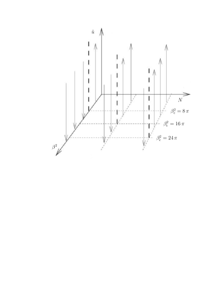
Figure 2: Renormalization-group trajectories for the effective coupling ${\tilde{u}}=k^{-2}\,u$ as a function of the number of layers $N$, according to the effective Lagrangian (34). The figure illustrates the generalization of Fig. 2 of Ref. [10] to an arbitrary number of layers.

In comparison to the previous investigations (WH approach used in Refs. [10, 6]), we here take a different route and perform first a rotation of the fields, before calculating the effective action as given in Eqs. (25) and (3). In the IR, the non-periodic mode can be treated perturbatively, by expanding the periodic interaction (cosine) in powers of the field. The fundamental coupling belonging to any non-periodic mode is found to have a trivial IR scaling, and the corresponding dimensionful quantities do not evolve at all under the RG transformations. This holds independently of the value of $\beta$, i.e. independently of the temperature. In the rotated Lagrangian, only one of the modes retains a mass term, and the determination of the general phase structure of the rotated model therefore becomes possible.

Generalizing a previous investigation [10], we find that the periodic mode in the $N$-layer structure actually undergoes a phase transition at a critical value of $\beta^{2}_{\rm c}=8N\pi$ (see Sec. 4). The effective $N$-layer Lagrangian for the periodic mode is given in Eq. (34). In addition to the obvious field-theoretic interest in related questions, the dependence on the number of layers finds a natural application in high-$T_{c}$ superconductors. As has already been stressed, the multi-layer sine-Gordon model can be considered as an adequate model for the vortex behaviour in layered superconductors (see Fig. 1 and Refs. [9, 13, 14]). The investigations presented here may indicate a possible explanation for the dependence of the transition temperature on the thickness of layered systems (see also Fig. 2). Experimentally, an increase of the transition temperature of high-$T_{c}$ materials with the number of layers has been observed [15]. Details of the mapping of $\beta^{2}_{\rm c}$ to the transition temperature, and of the transition to a three-dimensional model for an infinite number of layers, will be presented elsewhere.

Finally, with regard to the connection of the $N\to\infty$ limit to the three-dimensional case [6], we reemphasize that the the critical value becomes infinitely large in this limit ($\beta_{{\rm c},N}\to\infty$ for $N\to\infty$), and the model has only one phase. In this continuum limit, the multi-layer model can be considered as the discretized version of the three-dimensional sine-Gordon model (3D-SG), and the general result in Eq. (35) is therefore entirely consistent with the conclusions of Ref. [6]. In order to illustrate the mapping, we observe that the interlayer coupling term $J\,(\varphi_{i}-\varphi_{i+1})^{2}$, as given in Eq. (2), finds a natural interpretation as a kinetic term proportional to $(\partial\varphi/\partial z)^{2}$, in the limit $N\to\infty$. Of course, $z$ here denotes the third spatial direction, complementing the $x$ and $y$ integrations relevant for the Lagrangian (2).

References

• [1] W. Fischler, J. Kogut, L. Susskind, Phys. Rev. D19 (1979) 1188.
• [2] J. E. Hetrick, Y. Hosotani, S. Iso, Phys. Lett. B350 (1995) 92.
• [3] J. M. Kosterlitz, J. Phys. C7 (1974) 1046.
• [4] D. Amit, Y. Y. Goldschmidt, G. Grinstein, J. Phys. A13 (1980) 585.
• [5] I. Nándori, J. Polonyi, K. Sailer, Phys. Rev. D63 (2001) 045022.; Phil. Mag. B81 (2001) 1615.
• [6] I. Nándori, K. Sailer, U. D. Jentschura, G. Soff, Phys. Rev. D69 (2004) 025004; J. Phys. G28 (2002) 607.
• [7] T. Banks, D. Horn, H. Neuberger, Nucl. Phys. B108 (1976) 119.
• [8] M. B. Halpern, Phys. Rev. D12 (1975) 1684.
• [9] S. W. Pierson, O. T. Valls, Phys. Rev. B45 (1992) 13076; S. W. Pierson, Phys. Rev. Lett. 74 (1995) 2359; Phys. Rev. B55 (1997) 14536.
• [10] I. Nándori, S. Nagy, K. Sailer and U. D. Jentschura, Nucl. Phys. B 725 (2005) 467.
• [11] C. Itzykson and J. B. Zuber, Quantum Field Theory (McGraw–Hill, New York, 1980).
• [12] I. Nándori, submitted to J. Phys. A.
• [13] K. Vad, S. Mészáros, I. Nándori, B. Sas, e-print cond-mat/0508146 [Phil. Mag. (2006), at press]; K. Vad, S. Mészáros, B. Sas, Physica C432 (2005) 43.
• [14] I. Nándori, K. Sailer, e-print hep-th/0508033 [Phil. Mag. (2006), at press].
• [15] Y. Matsuda et al. Phys. Rev. B48 (1993) 10498; T. Ota et al. Phys. Rev. B50 (1994) 3363; J. Kötzler, M. Kaufmann, Phys. Rev. B56 (1997) 13734.