Probabilities in the inflationary multiverse
Abstract
Inflationary cosmology leads to the picture of a “multiverse,” involving an infinite number of (spatially infinite) post-inflationary thermalized regions, called pocket universes. In the context of theories with many vacua, such as the landscape of string theory, the effective constants of Nature are randomized by quantum processes during inflation. We discuss an analytic estimate for the volume distribution of the constants within each pocket universe. This is based on the conjecture that the field distribution is approximately ergodic in the diffusion regime, when the dynamics of the fields is dominated by quantum fluctuations (rather than by the classical drift). We then propose a method for determining the relative abundances of different types of pocket universes. Both ingredients are combined into an expression for the distribution of the constants in pocket universes of all types.
I Introduction
The fundamental theory of nature may admit multiple vacua with different low-energy constants. If there were just a few vacua, as in standard GUT models, then a few observations would determine which one corresponds to the real world. Predictions would then follow for every other observable in the low energy theory. However, it has recently been realized that in the context of string theory there may be a vast landscape of possibilities, with googols of vacua to scan duff ; Susskind ; Bousso . Many of these may look very much like our own vacuum, except for slight variations in the values of the constants. On the surface, this seems to undermine our ability for predicting these values, even after a systematic examination of the landscape.
Cosmology, on the other hand, suggests that rather than giving up on our ability to make predictions, we may in fact broaden their scope. Thus, instead of trying to determine from observations which vacuum is ours, we may try to determine, from the theory, what is the probability for the observation of certain values of the constants.111Note that this question is relevant even if the number of vacua is small. Indeed, eternal inflation AV83 ; Linde86 leads to the picture of a “multiverse,” where constants of nature take different values in different post-inflationary regions of spacetime. Observers bloom in such thermalized regions at places where the conditions are favorable, much like wildflowers at certain spots in the forest. Given a reference class of observers, we can ask what is the probability distribution for the values of the constants that they will measure. This approach was suggested in alex and further developed in GTV98 ; AV98 ; VVW ; GV01 . It leads to the following formal expression for the probability of observations,
| (1) |
is the volume fraction222 is sometimes referred to as the “prior distribution.” This name is motivated by Carter’s original discussion of anthropic selection in terms of Bayes’ rule. To avoid confusion with the usage of prior distributions in other contexts, here we shall simply call it the thermalized volume distribution. Note that the concept of a prior distribution for a set of parameters is also used when fitting observational data to a given model. There, the “prior” is often no more than a guess, representing our ignorance or prejudice about, say, the allowed range of the parameters. On the contrary, is here a quantity which should be calculable from the theory. of thermalized regions with given values of the constants , and is the number of observers in such regions per unit thermalized volume.333 is often referred to as the anthropic factor. Readers who dislike anthropic arguments are encouraged to think in terms of reference classes of their own choice.
Even though the dynamics responsible for the randomization of the constants during inflation is well understood, the calculation of probabilities has proven to be a rather challenging problem. The root of the difficulty is that the volume of thermalized regions with any given values of the constants is infinite (even for a region of a finite comoving size). To compare such infinite volumes, one has to introduce some sort of a cutoff. For example, one could include only regions that thermalized prior to some time and evaluate volume ratios in the limit . However, one finds that the results are highly sensitive to the choice of the cutoff procedure (in the example above, to the choice of the time coordinate LLM94 ; LLM+ ; see also Guth ; Tegmark for a recent discussion.) The reason for the cutoff dependence of probabilities is that the volume of an eternally inflating universe is growing exponentially with time. The volumes of regions with all possible values of the constants are growing exponentially as well. At any time, a substantial part of the total thermalized volume is “new” and thus close to the cutoff surface. It is not surprising, therefore, that the result depends on how that surface is drawn.
As suggested in GTV98 ; AV98 , this difficulty can be circumvented by switching from a global distribution, defined with the aid of some global time coordinate, to a distribution based on individual thermalized regions. The spacetime structure of an eternally inflating universe is illustrated in Fig. 1. The vertical axis is the proper time measured by comoving observers, and the horizontal axis is the comoving coordinate. Thermalized regions are marked by grey shading. Horizontal slices through this spacetime give “snapshots” of a comoving volume at different moments of (global) time. Initially, the whole volume is in the inflating state. While the volume expands exponentially, new thermalized regions are constantly being formed. These regions expand into the inflating background, but the gaps between them also expand, making room for more thermalized regions to form. The thermalization surfaces at the boundaries between inflating and thermalized spacetime regions are 3-dimensional, infinite, spacelike hypersurfaces. The spacetime geometry of an individual thermalized region is most naturally described by choosing the corresponding thermalization surface as the origin of time. The thermalized region then appears as a self-contained infinite universe, with the thermalization surface playing the role of the big bang. Following Alan Guth, we shall call such infinite domains “pocket universes.” All pocket universes are spacelike-separated and thus causally disconnected from one another. In models where false vacuum decays through bubble nucleation, the role of pocket universes is played by individual bubbles.
The proposal of Refs. GTV98 ; AV98 applies to the special case when all pocket universes are statistically equivalent. This happens, for instance, if there is only one low-energy vacuum, and the variation of the constants is due to long-wavelength fluctuations of some nearly massless fields. In this case, one may use any one of these pockets in order to calculate , which is then proportional to the volume fraction occupied by the corresponding regions in the pocket universe. This fraction can be found by first evaluating it within a sphere of large radius and then taking the limit .
Although the above proposal is conceptually satisfactory, it remains unclear how it should be implemented in practice. The most direct method, a numerical simulation, runs into severe computational limitations LLM94 ; VVW , and analytic methods have been developed only for very special cases. Moreover, if two or more vacua are mutually separated by inflating domain walls, then they cannot coexist in the same pocket universe. In this situation (which is expected to be quite generic in the landscape of string theory) there are distinct types of pocket universes, and we have to face the problem of comparing probabilities of different pockets. The purpose of the present paper is to try to improve on the approach of Refs. GTV98 ; AV98 ; VVW by addressing both of these issues.
In Section II we discuss an analytic estimate for the volume distribution of the constants within each pocket, based on the conjecture that the field distribution is approximately ergodic in the diffusion regime. When there are different types of pockets, the same approach can be used in order to find the internal volume distribution in a pocket of type . Then, in Section III, we introduce a new object which characterizes the relative abundance of each type of pocket universe. The aficionados may be aware of previous exploratory definitions of , which were nevertheless afflicted with certain drawbacks GV01 . For comparison, in Section IV we discuss one of these alternatives and in Section V we illustrate both definitions with some examples. Section VI discusses how the two objects and may be combined in order to find the full distribution for the constants. Our conclusions are summarized in Section VII.
II Probabilities within a pocket universe
II.1 Symmetric inflaton potential
The spacetime structure of a pocket universe is illustrated in Fig. 2. The surface in the figure is the thermalization surface. It is the boundary between inflating and thermalized domains of spacetime, which marks the end of inflation and plays the role of the big bang in the pocket universe. The surface is the boundary between the stochastic domain, where the dynamics of the inflaton field is dominated by quantum diffusion, and the deterministic domain, where the dynamics is dominated by the deterministic slow roll. Thus, marks the onset of the slow roll.
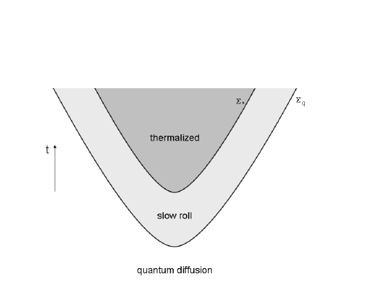
The surface is always spacelike. We shall assume that is spacelike as well. This can be arranged if is chosen not right at the diffusion boundary, but somewhat into the slow roll domain. We shall comment on the precise definition of at the end of Section II.C.
The probability for a variable is defined as the volume fraction on the thermalization hypersurface with given values of . It can be expressed as
| (2) |
where is the distribution (volume fraction) of on , and is the volume expansion factor during the slow roll in regions with the value . For simplicity, we shall identify the variable with the scalar field responsible for its value. Here, we have assumed that the diffusion of X can be neglected during the slow roll. We shall assume also that interacts very weakly with the inflaton, so that it does not change appreciably during the slow roll. Otherwise, we would have to include an additional Jacobian factor
| (3) |
in Eq. (2) AV98 . Here, and indicate, respectively, the time when slow roll begins and the time when observations are made.
The expansion factor can be found from
| (4) |
where is the inflaton field,
| (5) |
is the inflationary expansion rate, is the inflaton potential, the prime stands for a derivative with respect to , and we use Planck units throughout this paper. We denoted by and the values of at the boundary surfaces and , respectively. These values are defined by the conditions
| (6) |
and
| (7) |
The subscript in indicates that the value of where slow roll begins is generally -dependent, , and similarly for .
The distribution can in principle be determined from numerical simulations of the quantum diffusion regime. Some useful techniques for this type of simulation have been developed in LLM94 ; VVW ; VW . However, the simulations quickly run into computational limits, due to the exponential character of the expansion. Analytic techniques for the calculation of are therefore very desirable.
A special case where the analysis is trivial is the class of models where the potential is independent of in the diffusion regime. Then can be determined from symmetry,
| (8) |
An example is a “new” inflation type model with a complex inflaton, . Inflation occurs near the maximum of the potential at , and we assume in addition that the potential is symmetric near the top, . Equation (8) follows if this property holds throughout the diffusion regime. In such models, the distribution (2) reduces to AV98
| (9) |
Thus, the volume distribution is simply determined by the expansion factor during the slow roll.
In models where the inflaton potential does not have the assumed symmetry, the factor may provide an additional dependence on . We now turn to the discussion of this more general case.
II.2 Eternal inflation without thermalization
Let us first consider a model of eternal inflation without any low-energy vacua, where the dynamics is dominated by diffusion everywhere in the potential. The stochastic evolution of fields in the course of eternal inflation is described by the distribution function
| (10) |
where stands collectively for the inflaton and other light fields. This distribution satisfies the Fokker-Planck (FP) equation AV83 ; Starobinsky
| (11) |
where the flux is given by
| (12) |
Here,
| (13) |
is the diffusion coefficient,
| (14) |
is the “drift” velocity of the slow roll, and as before is the inflationary expansion rate.
The parameter in Eqs. (13) and (14) represents the freedom of choosing the time variable , which is assumed to be related to the proper time of comoving observers by
| (15) |
where the functions are taken along the observer’s world lines. Hence, corresponds to the proper time parametrization and corresponds to using the logarithm of the scale factor as the time variable. (We shall refer to the latter choice as the scale factor time.)
The FP equation is usually supplemented by boundary conditions at the thermalization boundary in -space, , where the conditions of slow roll are violated, and in some cases at the Planck boundary , where , and quantum gravity effects become important. Here, we shall assume that neither of these boundaries is present. For example, the -field space could be compact, with the potential satisfying and everywhere in this space. Then the fields will drift constantly from one value to another. The corresponding distribution has a stationary form with a vanishing flux,
| (16) |
With from (12), the solution of Eq. (16) is easily found Starobinsky . Up to a normalization constant, it is given by
| (17) |
Let us now use the scale factor time, , which corresponds to measuring time in units of the Hubble time . With this choice, Eq. (17) can be rewritten as
| (18) |
where
| (19) |
is the Gibbons-Hawking entropy of de Sitter space.
The solution (18) has a simple physical interpretation. The distribution can be thought of as representing observations by a comoving observer. The observer can see only her own horizon region (-region), and the value of should be understood as an average over that region. The quantum state of the -region is constantly changing due to de Sitter quantum fluctuations, and the average is also changing as a result. The distribution function is proportional to the fraction of time spent in quantum states with a given . The number of microscopic quantum states corresponding to a given value of is , and Eq. (18) indicates that, apart from the prefactor, the evolution during eternal inflation is ergodic, with all quantum states explored with an equal weight.
The prefactor suggests that at higher rates of inflationary expansion, the quantum state of an -region changes at a higher pace. The scale-factor time spent in each quantum state is (the proper time ). We note, however, that the prefactor in the solution (18) depends on the choice of ordering of the non-commuting factors and in the FP equation. In Eq. (12) above, we assumed the Ito factor ordering—the choice suggested by the phenomenological analysis in AV99 . A full microscopic derivation would require inclusion of quantum gravitational fluctuations, and until then the precise form of the prefactor will remain uncertain. We shall mostly disregard the prefactor in what follows.
The distribution (18) has an alternative interpretation, which will also be important for our analysis. It follows from the so-called physical-volume form of the FP equation GLM87 ; Sasaki ; LLM94 ,
| (20) |
Here, the function characterizes the distribution of physical volume between regions with different values of . More precisely, is the fraction of volume occupied by regions with in the intervals on hypersurfaces of constant . The flux is given by (12) with replaced by , and the last term in (20) accounts for the expansion of physical volume.
With , solutions of Eq. (20) and those of Eq. (11) are closely related LLM94 ,
| (21) |
This applies, in particular, to the solution (18). On surfaces of constant , the factor is a constant, and thus the volume distribution of along these surfaces is the same as the time distribution along the worldlines of comoving observers.
To appreciate the significance of this result, imagine dividing the spacetime into cells of size with . This can be done by first foliating the spacetime by surfaces of constant scale factor time, . The timelike separation between consecutive surfaces is of order . The next step is to divide the surface into cubes and to extend these cubes along comoving geodesics all the way to the surface . As a result, the spacetime layer between the surfaces and is divided into cells. This procedure is similar to laying bricks, starting with the surface , except that the bricks are somewhat irregular, with their tops being slightly bigger than their bottoms and their size depending on the local value of .
Now, we wish to know how is distributed among different cells. It follows from Eq. (21) that the distribution is given by (18), both in the time direction and in the spacelike directions along the surfaces . We can expect, therefore, that the 4-dimensional distribution of among the cells, that is, the distribution in a randomly picked volume, is still given by (18). Note that the form of the distribution does not depend on the choice of the spacelike hypersurface . This indicates that the distribution is not sensitive to the details of how the spacetime is divided into cells, as long as the cell sizes are set by the local horizon.
II.3 Ergodic conjecture
We now turn to the more physically interesting case, when inflation can end by thermalization in a low-energy vacuum. Here we shall assume that there is only one such vacuum, so that all thermalized regions are statistically equivalent. Each thermalized region has its own infinite hypersurface , which marks the boundary between quantum diffusion and slow roll. We are interested in the distribution on . Here, we have switched back from the notation to , where stands for one or several light fields.
The simplest guess is that has the same form as the distribution (18) in the diffusion region,
| (22) |
Here, as before, is the value of at the onset of the slow roll for given values of the fields . We do not have a proof that this guess is correct in general, but there are some special cases where the distribution (22) does seem to apply.
Suppose that the inflaton is trapped in a metastable false vacuum, . The false vacuum decays through bubble nucleation, which is followed by slow roll and thermalization, as in models of “open inflation” open . Prior to bubble nucleation, the evolution of the fields is governed by the stochastic dynamics described in the previous subsection. The corresponding probability distribution is
| (23) |
Once a bubble nucleates, the bubble wall expands rapidly with a speed approaching the speed of light, so the worldsheet of the wall closely follows the future lightcone of the nucleation point. The onset of slow roll surface will follow the same lightcone on the interior side of the bubble. If we imagine the spacetime divided into horizon-size cells with different values of , we can expect that the bubble will cut through a representative sample of cells and that the distribution of on will be given by (23). The distribution on the thermalization surface is obtained by multiplying (23) with the slow roll volume expansion factor, as in Eq. (2).
It should be understood that if the fields interact with the bubble, then the distribution (23) is processed as it goes through the bubble walls. This effect should be incorporated, just as the evolution of the fields during slow roll is incorporated in the Jacobian (3). In certain cases, the result of this processing can be easily estimated. For fields whose mass is much smaller than the inverse size of the bubble at the time of nucleation, the distribution inside the bubble takes the form quasiopen
| (24) |
Here, the subindex is used to denote that this is the distribution at the beginning of slow roll inside the bubble, right after nucleation. in the exponent is the action of the Coleman-de Luccia instanton describing bubble nucleation, and an adiabatic approximation is used for the Euclidean solution, where the field is assumed to take a constant value. In fact, all values of are realized at distant places inside any given bubble, but their distribution is still given by Eq. (24) quasiopen . Note that in the limit where there is no bubble, the Euclidean action is minus the entropy of de Sitter space, , and the expression (24) reduces to (23).
In cases where both and fields are in the diffusion regime prior to the slow roll, the situation is less clear. However, the following heuristic argument suggests that the distribution (22) may still approximately apply.
Consider an ensemble of comoving observers who start their evolution in regions where the fields are near the top of their potential. Most of these observers will get to the slow roll and thermalization after a relatively short period of diffusion. Only a small fraction of the observers will stay in the diffusion regime for much longer, but their respective regions will be expanded by a huge factor. This is the essence of eternal inflation: the histories of these “atypical” observers are, in a certain sense, more representative than those of the typical ones (after all, the thermalization surface is infinite thanks to the contribution of regions which linger in the diffusion regime for an indefinite amount of time.)
The measurements made by observers who spend a long time in the diffusion regime are described by the FP equation (11), supplemented by the constraint that the boundary between the diffusion and slow roll regions in the field space cannot be crossed. [The surface is defined by the condition (6).] Mathematically, this can be enforced by imposing the reflecting boundary condition on . The solution of the FP equation is then given by the stationary distribution (18). This indicates that, during diffusion, the observers will see ergodic evolution in their respective -regions.
We can thus argue, as in the previous subsection, that Eq. (18) describes the distribution in the quantum diffusion region of spacetime, which is in the past of the hypersurface . Then it appears plausible that the same distribution may extend, at least approximately, to the boundary with the slow roll region. This is the ergodic conjecture (22). It assumes that all quantum states corresponding to the field values on are equally represented by -regions on .
It should be noted that is defined by Eq. (6) only in the order-of-magnitude sense. This results in a significant uncertainty444This uncertainty is not present in models with bubble nucleation discussed earlier in this subsection. in the distribution (22), due to the exponential dependence on . A possible way of defining more precisely is the following. Suppose first there is a single inflaton and no other light fields. Surfaces of constant are spacelike in the slow roll regime, but not necessarily so in the diffusion regime. For in the diffusion regime, the surfaces have a complicated topology, while in the slow roll regime the topology is trivial. The transition between the two might be sharp, having the character of a phase transition. We could then define to be the critical value of . If there are several fields, the phase transition on the surfaces could be used to define .
II.4 An example
As an illustration, let us consider the potential
| (25) |
where is a very slowly varying function of the fields . Then
| (26) |
where , and Eq. (7) gives .
To make the condition (6) more precise, we rewrite it as
| (27) |
with , which yields
| (28) |
We shall assume that ; then .
The ergodic factor in Eq. (22) is given by
| (29) |
and the volume expansion factor is
| (30) |
We see that both factors are sensitive to the value of chosen to define . On the other hand, both factors have the form with , so we can be reasonably confident that the full distribution has this form, with a strong peak at the smallest allowed value of .
III Counting pockets
In models with pockets of several different types, we need to consider an additional factor characterizing the relative abundances of different types of pockets. Consider, for instance, a false vacuum which can decay into true vacua 1 or 2, with respective tunneling rates and . If , it seems intuitively clear that there will be more pockets of type 1 than of type 2 in the multiverse. This notion, however, should be made more precise.
In this section we propose a method for determining the relative abundances of different types of pockets. The counting is performed at the future boundary of spacetime—the place where everything has been said and done. Of course, the number of pockets of any given type is infinite, and a cutoff is needed. We shall argue that one such cutoff suggests itself naturally, and this allows us to perform an explicit calculation of the ’s. One can then examine different examples to check whether this is a reasonable prescription. As mentioned in the introduction, there have been in the past alternative proposals for which nevertheless are not very satisfactory. For comparison, one of these will be discussed in Section IV.
The full probability distribution should be obtained by combining the weights with the volume distributions in a suitable way. This will be discussed in Section VI.
III.1 Models with bubble nucleation
The string theory landscape is expected to have a multitude of high-energy metastable “false” vacua. Such vacua can decay through bubble nucleation. Bubbles of lower-energy vacuum nucleate and expand in the high-energy vacuum background. If the “daughter” vacuum has a positive energy density, then inverse transitions are also possible: bubbles of high-energy vacuum can nucleate in the low-energy one EWeinberg . (This is the so-called “recycling” process.) In both cases, the radius of the bubbles asymptotically approaches the comoving horizon size in the parent vacuum at the moment of nucleation recycling . In general, we will have multiple bubbles within bubbles within bubbles of many different types. The endpoints of this evolution are the negative or zero-energy vacua, which do not recycle. We shall call them terminal vacua.
Let be the fraction of comoving volume occupied by vacuum at time . The evolution equations for can be written as
| (31) |
where the first term on the right-hand side accounts for loss of comoving volume due to bubbles of type nucleating within those of type , and the second term reflects the increase of comoving volume due to nucleation of type- bubbles within type- bubbles. The transition rate is defined as the probability per unit time for an observer who is currently in vacuum to find herself in vacuum . It can be expressed as
| (32) |
where is the bubble nucleation rate per unit physical spacetime volume and is the expansion rate in vacuum . At this point, it will be convenient to distinguish between the inflating vacua, which we will label by Greek letters, and the terminal ones, for which we will reserve the indices and . Then, by definition,
| (33) |
We are interested in the number of nucleated bubbles of a given low energy vacuum (not necessarily a terminal one). As we know, the number of bubbles of all kinds grows without bound, even within a region of a finite comoving size. We thus need to cut off our count. The method we propose is to include only bubbles greater than some small comoving size . We will take the limit in our final result. Note that this cutoff prescription is independent of time parametrization. The comoving bubble size is set by the horizon at the moment of nucleation and remains constant in time. Our bubble counting can therefore be performed at future infinity. We shall call this the comoving horizon cutoff (CHC) method.
We can relate the number of bubbles nucleated in an infinitesimal time in the parent vacuum , , to the accompanying increase in comoving volume (which is the product of the number of bubbles and the comoving volume each bubble covers):
| (34) |
Here, is the Hubble constant of the parent vacuum, is the scale factor, and we have used the fact that the comoving radius of bubbles of any type nucleating in vacuum at time is
| (35) |
It will be convenient to use the scale factor time, . Then and
| (36) |
The comoving volume fractions can be found from Eq. (31), which can be written in a matrix form,
| (37) |
where and
| (38) |
The asymptotic solution of (37) at large has the form
| (39) |
Here, is a constant vector which has nonzero components only in terminal vacua,
| (40) |
It is clear from Eq. (33) that any such vector is an eigenvector of the matrix with zero eigenvalue,
| (41) |
As shown in Appendix B, all other eigenvalues of have a negative real part, so the solution approaches a constant at late times. We have denoted by the eigenvalue with the smallest (by magnitude) negative real part and by the corresponding eigenvector. It will also be shown in Appendix B that this eigenvalue is real and nondenegerate. This follows under the assumption that the set of inflating (nonterminal) vacua is “irreducible,” i.e. it cannot be split into groups of noninteracting vacua, where each vacuum from one group never nucleates any vacua from other groups. If there were such noninteracting groups, the present considerations would still apply to each group separately.
The asymptotic values of the terminal components depend on the choice of initial conditions. For any physical choice, we should have . Moreover, since can only increase with time, we must have
| (42) |
At the same time, we should have
| (43) |
because and . (Here, Eqs. (42) and (43) are justified on physical grounds. In Appendix B, these equations will be derived more rigorously.)
It follows from Eqs. (39), and (40) that Substituting this into (36) and integrating over , we obtain
| (44) |
The next step is to impose the cutoff. Our prescription is to include only bubbles of comoving size greater than . For bubbles of type nucleating in vacuum , this means that only bubbles nucleated prior to
| (45) |
should be included. With this cutoff, Eq. (44) gives
| (46) |
As expected, as . Our proposal is that ; hence,
| (47) |
The problem of calculating has thus been reduced to finding the dominant eigenvalue and the corresponding eigenvector .
We emphasize that our cutoff procedure is independent of coordinate transformations at future infinity. Any smooth change of coordinates will locally be seen as a linear transformation, which amounts to a constant rescaling of bubble sizes, accompanied by a rotation. Rescaling is generally different in different directions, so the shapes of the bubbles will be distorted from (approximate) spheres to ellipsoids. However, in a sufficiently small neighborhood of comoving size , all types of bubbles are distorted in the same way, so the bubble counting should not be affected by the distortion. (For a non-spherical bubble, the bubble size can be defined as its maximum extent, or the major axis of the ellipsoid.) The bubble density is dominated by the bubbles which formed at very late times, and which therefore have a very small comoving size. Hence, in any neighborhood of size the relative numbers of bubbles will not be affected by constant rescalings in the limit . This means that calculation of in any such neighborhood will give the same result, and it is clear that this result will also hold in a comoving region of any size.
III.2 Models with quantum diffusion
In quantum diffusion models, the calculation can be performed in a similar way, except the role of bubbles is now played by newly thermalized -regions. The rate at which the comoving volume thermalizes can be calculated by using the FP equation.
The FP equation for the distribution function applies in the region of -space outside the thermalization boundaries . The boundary condition on requires that diffusion vanish on LLM94 . In the notation of Sec. II.B,
| (48) |
where is the normal to .
The fraction of comoving volume which ends up in a thermalized region of type per unit time with the fields in an infinitesimal surface element of the thermalization boundary is given by
| (49) |
Using Eqs. (12) and (14) and the boundary condition (48), this can be expressed as
| (50) |
where .
The fraction of comoving volume that thermalizes during the scale factor time interval () is thus given by
| (51) |
The asymptotic comoving size of a pocket universe is much bigger than the comoving size of an -region at the time of thermalization. Let us denote by the ratio of these two sizes,
| (52) |
where is the time of thermalization. In fact, is of the order of the comoving size of the horizon at the time when slow roll begins, which is of order . Thus,555Regions in the vicinity of an region which has just entered slow roll, have field values which are also close to the boundary where slow roll begins, and so they are likely to cross it soon after. Because of such correlations, we expect that is somewhat larger than the comoving horizon size at the time , by a factor of a few, which can be determined from numerical simulations.
| (53) |
where is approximately given by (4). The number of pocket universes which begin thermalizing at time then satisfies
| (54) |
The asymptotic solution of the FP equation has the form
| (55) |
where is the smallest (by magnitude) eigenvalue of the FP operator. Substituting this in (54) and integrating over , we find the number of -regions that have thermalized up to time with in a given surface element . The probabilities are then found after a cutoff at and integration over ,
| (56) |
This equation allows us to calculate once we find the dominant eigenvalue and the corresponding eigenfunction . It should be noted that in the slow roll region, the diffusion term can be neglected and the Fokker-Planck equation becomes first order. One then readily finds that , where is the slow roll expansion factor. With given by (53), it is clear that the do not depend on where exactly we choose to define the thermalization boundary. The integrand can be evaluated anywhere in the slow roll regime, as long as diffusion is negligible. In fact, Eq. (56) is approximately valid if we substitute the subindex , corresponding to thermalization, by the subindex , indicating the onset of the slow roll regime. In this case . Note that the value of is typically very small.
In the preceding subsection we assumed that the physics of eternal inflation is described by bubble nucleation, and in the present subsection we assumed that it is described by quantum diffusion. The general case, when both mechanisms are present, can be described by combining the formalisms outlined in these subsections recycling .
IV Comoving probability
An alternative weight factor for the different types of pockets, , was used in Ref. GV01 . This is the so-called comoving probability, which can be defined as the probability for a comoving observer, starting near the top of the potential , to end up in a pocket of type . Let us now briefly describe, for comparison, the calculation of such probabilities.
IV.1 Models with quantum diffusion
The form of the FP equation depends on the time parametrization parameter , and the resulting distribution is, of course, also -dependent. However, as shown in AV99 , this distribution can be used to define reparametrization-invariant probabilities.
The probability for a comoving observer to end up in a thermalized region of type is given by
| (57) |
where the first integration is over . Again, using Eqs. (12) and (14) and the boundary condition (48), this can be expressed as
| (58) |
where we have introduced
| (59) |
Integrating the FP equation (11),(12) and the boundary condition (48) over time, we obtain the corresponding equations for :
| (60) |
| (61) |
Here, is the initial distribution at .
The function is uniquely determined by Eq. (60) with the boundary conditions (61). It can then be used in Eq. (58) to evaluate the probabilities . Note that the parameter has been absorbed in the definition (59) of and does not appear in Eqs. (58),(60),(61). This shows that this definition of is independent of time parametrization.
The physical origin of this reparametrization invariance is easy to understand. If we start with a large inflating volume at , different parts of this volume will thermalize into different minima of the potential, and at any time there will be parts of this volume that are still inflating. However, in the limit all the comoving volume will be thermalized, except a part of measure zero. Different choices of time parametrization affect the division of the volume into thermalized and still inflating regions, but this has no effect on , since the inflating regions represent only an infinitesimal part of the comoving volume at . In other words, the fraction of comoving volume that ends up in a given minimum of the potential is gauge-independent.
IV.2 Models with bubble nucleation
Likewise, in models with bubble nucleation it is convenient to introduce the new variable
| (62) |
Integrating Eq. (31) over time, we obtain
| (63) |
In the asymptotic future, all the comoving volume will be in the terminal vacua. Hence,
| (64) |
for all non-terminal vacua, whereas the probabilities for terminal vacua are given by
| (65) |
On the other hand, the initial distribution is concentrated at high-energy vacua; hence
| (66) |
Now, it follows from the above equations that
| (67) |
and
| (68) |
The quantities can be determined from (67), and the probabilities can then be found from Eq. (68). As before, the time reparametrization parameter has been absorbed in the definition of , and the probabilities do not depend on the choice of the time variable.
IV.3 Problems with
The probabilities in (58) and (68) are independent of time parametrization, but they do depend on the initial probability distribution or . We assumed that the initial distribution is concentrated near the maximum of the potential, or in the highest-energy false vacuum. However, if the potential has several peaks of comparable height, different values of will be obtained starting from different peaks.
It is possible that the initial distribution is to be found from the wave function of the universe, which determines the probability distribution for the initial states of the universe as it nucleates out of nothing. It is well known that, although inflating spacetimes are generically eternal to the future, all past-directed geodesics in such spacetimes are incomplete, except perhaps a set of measure zero (see BGV and references therein). This indicates that the inflating region of spacetime has a boundary in the past, and some new physics (other than inflation) is necessary to determine the initial conditions at that boundary. The prime candidate for the theory of cosmic initial conditions is quantum cosmology, which suggests that the universe starts as a small, closed 3-geometry and immediately enters the regime of eternal inflation.
If, for example, we adopt the tunneling wave function of the universe, the initial distribution is given by AV84 ; Linde84
| (69) |
This distribution favors large values of . So, if the potential is dominated by a single peak, the initial distribution will be concentrated at that peak.
The distribution (69) may be a plausible choice for the initial state of the universe, but the conclusion that the probabilities of different observations in an eternally inflating universe have some dependence on this choice appears to be counter-intuitive. Even though inflation must have had a beginning, one expects that once it began, the universe will quickly forget its initial conditions.
Another problem is that, from (64),
| (70) |
for all non-terminal vacua. If we use for determining the probabilities of being in different pockets, all non-terminal vacua are given zero probability. However, there seems to be no good reason to discard all such vacua. Note that the relative abundance of the corresponding pockets, discussed in the previous section, can be sizable. Also, our own low energy vacuum may have a small positive cosmological constant, in which case it would be non-terminal. This seems to disfavor the use of as a relevant weight factor.
The weight factors which we discussed in Section III do not suffer from these problems, and therefore seem more suitable for our present purposes.
V Some examples
We shall now use some examples to illustrate the similarities and differences between the weight factors and . Consider first a very simple model with one false vacuum and two terminal vacua and ( model). The allowed transitions in this model are shown by the “schematic”
| (71) |
The vector then has three components, , and the evolution equations (31) have the form
| (72) | |||
| (73) | |||
| (74) |
The first of these equations gives
| (75) |
with and
| (76) |
With the initial conditions , we have , and the other two equations yield
| (77) |
where . The comoving probabilities are defined by , which gives
| (78) |
This is in accord with the intuitive expectation: the probability of a vacuum is proportional to the nucleation rate of the corresponding bubbles.
We now compare this with the CHC (comoving horizon cutoff) approach. The transition matrix corresponding to Eqs. (72)-(74) has two zero eigenvalues with eigenvectors and , and a negative eigenvalue [where is given by Eq. (76)] and eigenvector . For our model, the sum in Eq. (47) has only one term (the one with ), and the only -dependent factor in (47) is . Thus, the CHC prescription gives
| (79) |
in agreement with Eq. (78).
We next consider a model with an intermediate vacuum between and ,
| (80) |
( model). Bubbles of and nucleate in , but bubbles of are themselves sites of eternal inflation, with an infinite number of -bubbles nucleating in each of them. This model illustrates the difference between the weight factors and .
The evolution equations for the model are
| (81) | |||
| (82) | |||
| (83) | |||
| (84) |
Once again, we start with the comoving probabilities. The solution of Eqs. (81)-(84) with the initial conditions is
| (85) | |||
| (86) | |||
| (87) | |||
| (88) |
where
| (89) |
and
| (90) |
The comoving probabilities for this model are
| (91) |
This result is easy to understand. We start with all comoving volume in . This volume is then divided between the bubbles of and in the ratio . All the comoving volume in -bubbles is eventually turned into -bubbles, and thus the ratio of comoving volumes in and is given by (91).
Let us now compare this with the CHC method. The matrix for the model has two nonzero eigenvalues: with from (89) and with . The corresponding eigenvectors are
| (92) |
and
| (93) |
The asymptotic behavior of the model depends on the relative magnitude of and .
For , or
| (94) |
is the dominant eigenvalue, and Eq. (47) gives
| (95) |
Conversely, if , then is the dominant eigenvalue, and we find
| (96) |
Once again, these results are easy to understand. For , the high-energy vacuum decays faster than the intermediate vacuum . So, in the asymptotic regime the comoving volume is divided between bubbles of and , and each bubble of still continues to produce bubbles of . As a result, -bubbles are completely outnumbered by -bubbles. In the opposite limit, when , turns into very quickly, and in this sense the model is not very different from the model. In this limit, Eq. (95) gives , in agreement with (91).
It is not difficult to extend this analysis to the case where the intermediate vacuum is recyclable, so the schematic is . This is done in Appendix A.
We thus see that both weight factors and give results which are in agreement with intuitive expectations. A priori, it is not clear which one of these two objects is more useful for the purposes of defining probabilities for the constants of nature. Progress can be made by working out their values in a variety of models, to see which, if any, of the two can be included in a reasonable definition of probabilities. As discussed in the previous section, it appears that on general grounds the are preferable. This is because of their independence of the initial conditions, and because they assign non-vanishing probabilities to non-terminal vacua (unlike the co-moving probabilities). Also, the example considered in this section indicates that in models where there are intermediate vacua which are also eternally inflating, the probabilities seem to better represent the actual distribution of terminal pockets and . Hence, in what follows, we shall concentrate on .
VI The full distribution
Let us now address the question of calculating probabilities for observations in the case when there are different types of pockets. The full probability distribution may be written as
| (97) |
where is defined as the number of observers that will evolve per unit comoving volume with specified values of the fields , and is a local time variable in a pocket of type . The calculation of will not be discussed in this paper, and we shall simply assume that, given the reference class of observers, this can be calculated from first principles. The distribution should represent the physical volume fraction in pockets of type , with specified values of the fields . Within a given pocket, the quantities and should be calculated at the same time , but it is not important which moment of time and which time variable we choose. The volume grows and the density decreases with the expansion, but of course the product does not change. (Note that includes all observers—present, past, and future—that will ever evolve in a comoving volume having unit size at , so its -dependence is simply , where is the scale factor.)
In Ref. GV01 an attempt was made to compare the volumes in different pockets. The idea was to quantify the amount of expansion measured from the inflaton’s last visit to the highest point in its potential. For that purpose, some fictitious markers were introduced, which were produced at a constant rate in regions where the field is at the top of the potential, and which where subsequently diluted. The mean separation of the markers in the different thermalized regions would then indicate how much expansion intervened since the field was at the top. This method runs into some conceptual problems. If there are several peaks of comparable height in the potential, then it is not clear why we should only count one of them as the source of markers. Also, since markers are only produced at a very special field value, all field values which are distant from it get rewarded with a large expansion factor, for no particularly compelling reason. In the face of such difficulties, one option would be to content ourselves with the volume distributions for individual pockets as the last frontier of predictivity.
Nevertheless, the structure of the eternally inflating spacetime is well understood, and we feel that a useful characterization of the relative likelihood the constants of nature in pockets of different types can be obtained from the distributions and which we have considered in the previous sections.
Let us start, for simplicity, with the case where the different pockets are generated by bubble nucleation. Suppose also that different pockets have different values of the constants, but that these constants do not vary within a given bubble. Our goal is to determine the probability of being in a given pocket , . In this case, the problem is that of combining and into [for the time being, there is no to worry about, since the constants do not vary within a given pocket].
For that, we need to define a co-moving reference scale specifying the size of the regions in which the observers are to be counted, and we can write
| (98) |
where is the physical size of the reference scale and we have omitted the subscript of . To determine , we note that at early times, the dynamics of the open FRW universe inside a bubble is dominated by curvature, and we have for all types of bubbles. Later on, when the curvature scale grows to the size of the Hubble radius associated to the corresponding local energy density, the curvature dominated phase gives way to slow roll inflation inside the bubble. For a quasi-de Sitter slow roll phase we would have
| (99) |
where is the Hubble rate at the beginning of the slow roll. The specific form of the scale factor at late times is not important for our argument. The point is that for times much smaller than the onset of slow roll, , all pockets are nearly identical, with scale factor . This suggests that the reference scales should be chosen so that is the same in all pockets at some . Then, up to a constant,
| (100) |
For times this can be expressed as , where is the redshift factor from the time at which slow roll begins. Alternatively, we note that is the comoving curvature scale, which can be defined without any reference to .
Now, this can be straightforwardly generalized to the case when there are some continuous variables , by simply including the factor —the normalized distribution for on the surface :
| (101) |
The volume distribution of on the surface is
| (102) |
where we abreviate , and is the normalization factor
| (103) |
Combining the above equations, the fraction of volume in pockets of type with values of the constants takes the form
| (104) |
Here, is the single pocket volume distribution normalized at the onset of slow roll (in the case of diffusion, this can be estimated as the ergodic factor , or using Eq. (24) in the case of bubble nucleation). The factor has the dimension of volume. From (102) we have . The left hand side of this equation is normalized to unity, and therefore we may write in terms of the volume distribution on ,
| (105) |
Note that the product featuring in the denominator of is the number distribution of -regions on with the given value of in pockets . An alternative form of (104) is given in terms of this number distribution by
| (106) |
where is normalized on . This result has a simple intuitive interpretation. The volume distribution is proportional to the relative number of pockets of a given type , times the relative number of Hubble regions within these pockets with given values of , , on the surface where slow roll starts, times the volume of these regions , times the subsequent growth factor .
Our derivation of (104), or its equivalent form (106), has been based on the case of bubbles, but it is possible to adopt the same prescription also for the case of pocket universes generated by diffusion, since the result only makes reference to the surface where slow roll begins and to the subsequent expansion thereof.
At present, we cannot claim that the prescription we have introduced here is the only consistent one. However, the hope is that from the careful analysis of a sufficiently wide range of possibilities a unique prescription will emerge. To illustrate this point, let us consider two alternatives which on the surface may seem reasonable.
Let us first consider a possibility which we shall refer to as Alternative . This consists of identifying with the volume fraction in pockets of type . In this case, we would have
| (107) |
Here, is the distribution normalized on the corresponding thermalization boundary,
| (108) |
Although the choice (107) may appear reasonable at first sight, it is unsuitable for substitution into Eq. (97). Indeed, the product should be independent of the time at which we choose to calculate it. But with the present choice, stays constant, while dilutes with the expansion.
To avoid this problem, we may then think of another possibility, which we shall refer to as Alternative , where
| (109) |
Here, it is which is normalized to one. With this, the time at which we calculate is unimportant, since this product is independent of time. This proposal, however, does not take the form (97) and contradicts our starting point that all members of the reference class of observers carry equal weight (which is in fact the very definition of reference class). Suppose we have a single false vacuum decaying into two types of bubbles with equal nucleation rates, so that . The vacuum in type-1 bubbles is very hospitable to observers, while the vacuum in type-2 bubbles is almost lethal and density of observers is strongly suppressed. One expects that observers are much more likely to find themselves in a type-1 bubble. However, after the normalization prescribed in (109), we would conclude that we are equally likely to be in either type of bubble. The basic problem here is that the factors are determined by the transition rates, or by the diffusion dynamics, and therefore they will be insensitive to the amount of slow roll inside of a given pocket—and much less to the number of observers which will subsequently develop. Hence, we must also reject this alternative.
The preceeding discussion illustrates that, as we have seen in the case of Alternatives and , certain reasonably-looking prescriptions can be discarded after careful consideration of their consistency. Another way of narrowing down the possibilities is by working out their predictions and comparing them with the data.666This type of analysis has already proved useful when applied to definitions of probability based on a constant-time cutoff. For a wide class of time variables, such definitions lead to absurd predictions that we should find ourselves in a deep, nearly spherical gravitational potential well LLM2 and that the CMB temperature should be many orders of magnitude higher than observed Tegmark . (As we mentioned in the Introduction, another objection against constant-time cutoffs is that they rely on an arbitrary choice of the time variable.) Although a full analysis is beyond the scope of the present paper, we believe that the definition (104) [or equivalently (106)] is the most appealing amongst those which we have considered, and has the best chance of being correct.
VII Summary and discussion
In the context of theories with many vacua, such as the landscape of string theory, the low energy constants of Nature are randomized during inflation, and will vary from place to place in the thermalized post-inflationary regions. An interesting question is then to find the volume distribution of the constants in such thermalized regions. In this paper, we have developed some tools towards this goal.
The problem splits into two parts. First of all, we should find the distribution of constants within a given pocket universe. Following up on the approach of Refs. AV98 ; VVW , we have motivated an analytic estimate for this distribution. According to Eq. (2), the internal volume distribution in a given pocket of type takes the form
| (110) |
where and are the distribution at the onset of slow roll and the slow roll expansion factor respectively. We argued in Section II.C that
| (111) |
This is what we called the ergodic conjecture.777In models of bubble nucleation followed by slow roll inside the bubble, Eq. (111) should be replaced with an expression of the form (24). It should be understood that our justification of (111) has been rather heuristic, and the limits of its validity should be further explored.
Next, we have introduced a weight factor which counts the relative number of pockets of type . The counting is done at the future boundary of spacetime, by considering all pockets of comoving size larger than some , and then letting . We have called this the comoving horizon cutoff (CHC), since the comoving size of a pocket is roughly given by the size of the horizon at the time when the pocket is formed. As we explained at the end of Section III.A, such a cutoff is independent of coordinate transformations at the future boundary.
For comparison, we have also discussed an alternative weight factor , defined in GV01 as the fraction of comoving volume which ends up in pockets of type . Unlike the ’s discussed above, the comoving volume fraction strongly depends on initial conditions. Moreover, all co-moving volume ends up in terminal vacua (these are vacua which cannot further decay into other vacua). Because of that, all non-terminal vacua are assigned zero probability. However, there seems to be no good reason to discard all such vacua, since the relative abundance of the corresponding pockets can be sizable. Also, our own low energy vacuum may have a small positive cosmological constant, in which case it would be non-terminal. Because of these two problems, the probabilities seem less relevant for our present purposes.
In the case where all terminal vacua emanate directly from a single eternally inflating false vacuum, we find that the weight factors and agree with each other, and they are basically proportional to the corresponding nucleation rates. The differences between and are illustrated in a model where there is an intermediate false vacuum which is also eternally inflating. Again, the weight factors seem to give a better representation of the actual distribution of pockets in the multiverse.
We have combined the above distributions into an object describing the thermalized volume distribution of the constants of nature in the inflationary multiverse with pockets of different types. If these constants are determined by the values of certain light fields , then we have argued that the volume fraction occupied by values in pockets of type is given by
| (112) |
Here, is the boundary (in field space) where quantum diffusion turns into classical slow roll. The factor , whose calculation is discussed in Section III, takes into account the relative numbers of pockets of type . The quantity is the number distribution of Hubble-size regions with values of the fields within pockets of type at (see Fig. 2 for the space-time structure of a pocket universe), and is the volume of one such region. According to the ergodic conjecture, this distribution is essentially given by Eq. (111) [or Eq. (24) in the case of bubbles]. The hat on indicates that it is normalized as . is the expansion factor from the point on to the thermalization boundary , along the classical slow roll trajectory.
Although our proposal for comparing the probabilities in pockets of different types seems to be well motivated, it may not be the unique possibility. Settling this issue may require further research. For comparison, we have also explored some alternatives. In the first one, the weight factor is formally identified with the volume fraction in pockets of type , and in the second one, is formally identified with the fraction of observers in pockets of type . We have shown that both of these options would lead to inconsistencies.
With the analytic approximations we have suggested, the distribution (112) can be readily calculated in a variety of models. The probability distribution for the measurements of observers in a given reference class can be obtained by substituting (112) into Eq. (97). Application to examples which may be relevant to the landscape of string theory (such as the Bousso-Polchinski scenario Bousso ) is left for further research.
Acknowledgments
J.G. is partially supported by grants FPA 2004-04582-C02-02 and DURSI 2001-SGR-0061. A.V. is partially supported by the NSF.
Note added
After this paper was submitted, Easther, Lim, and Martin (ELM) suggested an alternative prescription for computing the weights assigned to different types of pocket universes ELM05 . In this note we show that their prescription is equivalent to the CHC method.
The ELM prescription is formulated for a model with bubble nucleation, and we shall restrict our attention to that case. The main problem of counting bubbles is to select a large but finite subset from the infinite set of all the bubbles created during the infinitely long evolution. Once a finite subset is selected, the probability ratio is found as the ratio of the number of bubbles of types and from the subset, in the limit of large subset size. The ELM proposal consists of choosing a large but finite number of randomly drawn comoving worldlines and selecting the subset of bubbles that intersect at least one of these worldlines. The distribution of worldlines is assumed to be statistically independent of the bubble nucleation process. Then the resulting weights are independent of the choice of worldlines.
The subset of bubbles selected by the ELM prescription differs from the subset selected by the CHC method because some bubbles in the ELM subset may have an arbitrarily small comoving size. However, we shall now show that the ELM prescription produces the same result for as the CHC method, for a generic bubble nucleation model (with or without recycling).
The above mentioned assumption of statistical independence (“the worldlines do not know about the pockets”) is equivalent to assuming that there exists a well-defined probability density for a randomly chosen worldline from the congruence to end in a bubble of type at a time . Let us draw the worldlines uniformly with a constant probability per unit comoving 3-volume; this is an admissible distribution in the sense of the ELM prescription. Then is equal to the probability of nucleating a bubble of type at time at a randomly chosen comoving point. It is clear from Eq. (31) that
| (113) |
where the index spans only the non-terminal vacua.
To simplify the calculation, we consider a uniform cubic grid of worldlines where all the cubes have sides . Then the smallest and the largest (comoving) distances between neighboring worldlines are and . This is again an admissible congruence of worldlines, chosen independently of the bubble nucleation process. The subset of bubbles selected by the ELM prescription will include all bubbles of comoving size (the counting of which constitutes the CHC prescription), as well as some bubbles of smaller comoving size. So it remains to show that the additional counting of bubbles of smaller size will not influence the CHC result, in the limit .
The total number of selected bubbles with sizes is no greater than the number of worldlines that do not intersect larger bubbles of size . It follows from Eqs. (39), (113), and the condition , that the probability of a worldline encountering a bubble at late times is exponentially small, . Due to Eq. (45), the limit corresponds to the limit . Hence, the additional counting of smaller-size bubbles produces an exponentially small correction to the CHC counting, and this correction disappears as . Therefore, we have recovered the CHC bubble counting result in the limit . Since the ELM prescription is insensitive to the distribution of the worldlines, we conclude that the two prescriptions always yield identical results.
Appendix A: FABI model with recycling
We now consider a version of the model which includes recycling between vacua and as indicated in the schematic .
Writing out the master equation, we obtain:
| (114) | |||
| (115) | |||
| (116) | |||
| (117) |
We will first consider the comoving probabilities. Noting that we take to be independent of time, we can integrate equations (114) to (117) from some initial time to to obtain
| (118) | |||
| (119) | |||
| (120) | |||
| (121) |
where we have defined
| (122) |
For simplicity we also define
| (123) | |||
| (124) | |||
| (125) | |||
| (126) |
Solving this system of linear equations for in terms of the initial conditions and the transition rates, we find the ratio of comoving probabilities as
| (127) |
with related to the transition rates as given in Eqs. (123)-(126).
For the initial condition , we have
| (128) |
We now compare this result with the CHC method. We solve for the eigenvalues and eigenvectors of , yielding explicit expressions for the . The result is
| (130) | |||
| (131) | |||
| (132) | |||
| (133) | |||
| (134) |
where
| (135) |
is the dominant eigenvalue, and is the corresponding eigenvector. For completeness we note that the other nonzero eigenvalue (call it ) is given by
| (136) |
and that this differs from only by the sign of the square root term.
If we now want to calculate the probabilities in the limit that (that is, we assume that recycling from back into is nearly negligible), we can Taylor expand about . We find
| (137) |
Using Eq. (47) we find as ,
| (138) |
if and
| (139) |
if , in agreement with the results of Section V, where was neglected from the very beginning.
Appendix B: Nondegeneracy of the subleading eigenvalue
In this appendix we study the mathematical properties of the matrix defined by Eq. (38). Formulations and proofs of some technical lemmas will be deferred until the end of this appendix. We shall show that all nonzero eigenvalues of have negative real parts, and that the subleading eigenvalue of the matrix is real and nondegenerate, under the following assumptions:
I. The set of all the inflating (nonterminal) vacua cannot be split into disconnected groups, where each vacuum from one group never nucleates any vacua from other groups.
II. Transitions between any two inflating vacua are reversible: If , then as well.
III. There exist transitions to some terminal vacua with nonzero rates.
We begin by considering the vector of comoving volume fractions which satisfies Eq. (37),
| (140) |
where the matrix elements of are defined by
| (141) |
Conservation of the comoving volume requires that the sum of any column of be equal to zero. It follows from this condition that all eigenvalues of have nonpositive real parts (see Lemma 1 below).
Suppose that there are inflating vacua and terminal vacua. We can split the vector into a direct sum of two vectors, and , representing the volume fractions in these two types of vacua. Then Eq. (140) can be rewritten as a system of two vector equations,
where the matrix describes the transition rates between the inflating vacua and describes the transition rates from inflating to terminal vacua. Thus the matrix has the following block appearance,
| (142) |
Note that the matrix is square with dimensions , while the matrix has dimensions and may not be square.
We already know that the matrix has a zero eigenvalue and no positive eigenvalues. We shall now prove, under the assumptions I-III above, that the eigenvalue of with the algebraically largest real part is a nondegenerate and negative eigenvalue .
It follows from the assumptions I and II that any inflating vacuum will eventually nucleate bubbles with any other inflating vacuum (either directly or after passing through bubbles of other inflating vacua). The technical term for this property is that the matrix is irreducible: for any indices there exist a chain of indices such that all the matrix elements are nonzero.
Let us now analyze the eigenvalues of in general. Any eigenvector of has either all zero inflating components, i.e. it is a vector of the form , or with . All vectors of the form are obviously eigenvectors of with eigenvalue , while eigenvectors of the form such that must satisfy . We shall shortly demonstrate that all eigenvalues of the matrix have negative real parts and that the maximal eigenvalue of is real, negative, and nondegenerate, while the corresponding eigenvector can be chosen with all positive components. It will then follow that the subleading eigenvalue of is equal to and is nondegenerate, and the corresponding eigenvector of is . Note that the components of the matrix are nonnegative, and thus the inflating components of the vector have the opposite sign as compared with the terminal components. This confirms our earlier statements (42) and (43).
Now we shall show that all eigenvalues of the matrix have strictly negative real parts. Since is irreducible and has nonnegative off-diagonal components, there exists a nondegenerate eigenvalue of with the largest real part (the maximal eigenvalue) and all other eigenvalues have a smaller real part (see Lemma 1). By construction, the matrix is of the form (141), where the indices are restricted to the range . It follows from the assumption III that the sums of each column of are not all equal to zero and thus
| (143) |
Then it follows from the estimate (150) of Theorem 1 that . However, we would like to prove the strict inequality . To this end, we shall assume that and arrive to a contradiction. If , there exists an (-dimensional) eigenvector with all positive components (Lemma 1) such that . We can now express the matrix as a difference of a matrix having vanishing sums of each column, and a diagonal matrix whose entries are nonnegative, namely
| (144) | ||||
| (145) | ||||
| (146) |
Here the matrix describes the nucleation of inflating vacua and the matrix describes the nucleation of terminal vacua. The equality then yields
| (147) |
Since all the components of are positive, and since and by assumption III, we conclude that not all components of the vector are zero:
| (148) |
Note that the matrix definitely has a zero eigenvalue since the sums of all columns vanish. Applying Lemma 1 to the matrix , we find that the maximal eigenvalue of is , and since the matrix has a zero eigenvalue, this eigenvalue must be maximal, i.e. . Intuitively, we expect that this maximal eigenvalue is diminished when we subtract a nonnegative and nonzero matrix from . Indeed, Lemma 3 shows that the existence of a positive vector satisfying means that is the eigenvector of corresponding to , in other words, we have , which contradicts Eq. (148). Therefore the matrix cannot have an eigenvalue .
Finally, we list some statements used in this appendix. A matrix (or a vector) is called nonnegative if all components are nonnegative. We write for vectors if for all .
Theorem 1: A nonnegative matrix has a real eigenvalue such that all other eigenvalues , are smaller than in magnitude, . If the matrix is irreducible, then the eigenvalue is nondegenerate and the corresponding eigenvector can be chosen with all positive components. Furthermore, if we denote
| (149) |
then the largest eigenvalue is bounded by
| (150) |
This is the Perron-Frobenius theorem and its corollary. For a proof, see Lanc69 , chapter 9, and also Minc88 , chapter 1.
Lemma 1: If a matrix is irreducible and for , then there exists a nondegenerate real eigenvalue of such that the corresponding eigenvector has all positive components, and all other eigenvalues have smaller real parts, (maximal eigenvalue). Moreover, if for all , then .
Proof: We can choose a real number such that the auxiliary matrix is nonnegative. The matrix is irreducible and thus, by Theorem 1, has an eigenvalue such that the corresponding eigenvector has all positive components, and all other eigenvalues lie within the circle ; hence, . Since the eigenvalues of are , the first statement follows. The second statement follows from the estimate in Theorem 1, which yields
| (151) |
hence .
Lemma 2: If is a nonnegative irreducible matrix, and if is the maximal eigenvalue of from Lemma 1, and if there exists a nonnegative vector such that , then is an eigenvector of with eigenvalue .
A proof of this technical statement is contained in the proof of Theorem 4.1 in Ref. Minc88 , chapter 1.
Lemma 3: If a matrix is irreducible and for , and if is the maximal eigenvalue of from Lemma 1, and if there exists a nonnegative vector such that , then is an eigenvector with eigenvalue .
Proof: We consider the auxiliary nonnegative matrix as in the proof of Lemma 1. It follows that . We note that is the maximal eigenvalue of . Now Lemma 2 can be applied to the matrix and it follows that is an eigenvector of with eigenvalue .
References
- (1) R. Bousso and J. Polchinski, JHEP 0006, 006 (2000) [arXiv:hep-th/0004134].
- (2) M. J. Duff, B. E. W. Nilsson, and C. N. Pope, Phys. Rept. 130, 1 (1986).
- (3) L. Susskind, arXiv:hep-th/0302219.
- (4) A. Vilenkin, Nucl. Phys. B 226, 527 (1983).
- (5) A. D. Linde, Phys. Lett. B 175, 395 (1986).
- (6) A. Vilenkin, Phys. Rev. Lett. 74, 846 (1995).
- (7) J. Garriga, T. Tanaka, and A. Vilenkin, Phys. Rev. D 60, 023501 (1999) [arXiv:astro-ph/9803268].
- (8) A. Vilenkin, Phys. Rev. Lett. 81, 5501 (1998) [arXiv:hep-th/9806185].
- (9) V. Vanchurin, A. Vilenkin, and S. Winitzki, Phys. Rev. D 61, 083507 (2000) [arXiv:gr-qc/9905097].
- (10) J. Garriga and A. Vilenkin, Phys. Rev. D 64, 023507 (2001) [arXiv:gr-qc/0102090].
- (11) A. D. Linde, D. A. Linde, and A. Mezhlumian, Phys. Rev. D 49, 1783 (1994) [arXiv:gr-qc/9306035];
- (12) A. D. Linde, D. A. Linde, and A. Mezhlumian, Phys. Lett. B 345, 203 (1995) [arXiv:hep-th/9411111]. A. D. Linde and A. Mezhlumian, Phys. Rev. D 53, 4267 (1996) [arXiv:gr-qc/9511058]; J. Garcia-Bellido and A. D. Linde, Phys. Rev. D 51, 429 (1995).
- (13) A. H. Guth, Phys. Rept. 333, 555 (2000) [arXiv:astro-ph/0002156].
- (14) M. Tegmark, JCAP 0504, 001 (2005) [arXiv:astro-ph/0410281].
- (15) S. Winitzki and A. Vilenkin, Phys. Rev. D 61, 084008 (2000) [arXiv:gr-qc/9911029].
- (16) A. A. Starobinsky, in Current Topics in Field Theory, Quantum Gravity and Strings, Lecture Notes in Physics, edited by H.J. de Vega and N. Sanchez (Springer, Heidelberg, 1986).
- (17) A. Vilenkin, Phys. Rev. D 59, 123506 (1999) [arXiv:gr-qc/9902007].
- (18) A. S. Goncharov, A. D. Linde, and V. F. Mukhanov, Int. J. Mod. Phys. A 2, 561 (1987).
- (19) K. Nakao, Y. Nambu and M. Sasaki, Prog. Theor. Phys. 80, 1041 (1988); Y. Nambu and M. Sasaki, Phys. Lett. B219, 240 (1989).
- (20) J. R. Gott, Nature 295, 304 (1982); M. Bucher, A. S. Goldhaber, and N. Turok, Phys. Rev. D 52, 3314 (1995) [arXiv:hep-ph/9411206]; K. Yamamoto, M. Sasaki, and T. Tanaka, Astrophys. J. 455, 412 (1995) [arXiv:astro-ph/9501109].
- (21) J. Garcia-Bellido, J. Garriga, and X. Montes, Phys. Rev. D 57, 4669 (1998) [arXiv:hep-ph/9711214].
- (22) K. M. Lee and E. J. Weinberg, Phys. Rev. D 36, 1088 (1987).
- (23) J. Garriga and A. Vilenkin, Phys. Rev. D 57, 2230 (1998) [arXiv:astro-ph/9707292].
- (24) A. Borde, A. H. Guth, and A. Vilenkin, Phys. Rev. Lett. 90, 151301 (2003) [arXiv:gr-qc/0110012].
- (25) A. Vilenkin, Phys. Rev. D 30, 509 (1984).
- (26) A. D. Linde, Lett. Nuovo Cimento 39, 401 (1984).
- (27) A.D. Linde, D.A. Linde and A. Mezhlumian, Phys. Lett. B345, 203 (1995).
- (28) P. Lancaster, Theory of matrices, Academic Press, NY, 1969.
- (29) H. Minc, Nonnegative matrices, Wiley, NY, 1988.
- (30) R. Easther, E. A. Lim, and M. R. Martin, preprint astro-ph/0511233.