Implicit Regularization and Renormalization of QCD

Abstract

We apply the Implicit Regularization Technique (IR) in a non-abelian gauge theory. We show that IR preserves gauge symmetry as encoded in relations between the renormalization constants required by the Slavnov-Taylor identities at the one loop level of QCD. Moreover, we show that the technique handles divergencies in massive and massless QFT on equal footing.

I Introduction and basics of Implicit Regularization

Dimensional Regularization (DR) is the natural framework for computing Feynman diagrams in gauge field theories. However the regularization of dimension specific quantum field theories such as chiral, topological and supersymmetric gauge theories is known to be a delicate matter in the context of DR. That is because the analytical continuation on the space-time dimension of the Levi-Civita tensor is not well-defined whereas supersymmetry is intrinsically defined on the physical dimension of the underlying model.

Although some extensions of DR have been constructed (e.g. Dimensional Reduction Siegel ) they are in general inconsistent in arbitrary loop order and may give rise to spurious anomalies. Hence a judicious order by order calculation in which the symmetry content of the model is assured via constraint equations has to be performed. The drawbacks are clear: in addition to turning the calculations cumbersome and tedious, we cannot rely on such procedure to study anomalous (quantum mechanical) symmetry breaking. This is particularly relevant in the supersymmetric extensions of the standard model Jack .

This motivates the search for a non-dimensional regularization/renormalization scheme which, besides preserving the vital symmetries of the quantum field theoretical model, is friendly from the calculational viewpoint.

Implicit Regularization (IR) is a momentum space setting to perform Feynman diagram calculations in regularization independent fashion. The Lagrangian of the underlying quantum field theory is not modified: neither an explicit regulator is introduced nor the dimensionality of the space time is moved away from its physical dimension. It has been successfully applied to various quantum field theoretical models including those which make sense only in their physical dimension. For quantum eletrodynamics, theories involving parity violating objects (Chern-Simons, Chiral Schwinger Model), see PRD1 . For the study of anomalies and CPT violation in an extended chiral version of quantum electrodynamics see PRD2 . A comparison between IR, dimensional regularization, differential renormalization and BPHZ forest formula can be found in PRD3 , where it is also calculated the beta function to one loop order in quantum chromodynamics. In NLOOP a model calculation using $\phi^{3}$ theory in $6$ dimensions illustrates how IR works when overlapping divergencies occur. In JHEP it is shown that IR is manisfestly supersymmetric invariant. This is illustrated by renormalizing the massless Wess-Zumino model and calculating the beta function to three loop order. Application to a Gauged Nambu-Jona Lasinio model can be found in CO .

The main idea behind IR is very simple. The ultraviolet behaviour of the amplitude is isolated as irreducible loop integrals (ILI’s) which are independent of the external momenta and need not be explicitly evaluated to display the physical content of such amplitude. This can be achieved by judiciously using the identity at the level of the integrand

$$\frac{1}{[(k+k_{i})^{2}-m^{2}]}=\sum_{j=0}^{N}\frac{(-1)^{j}(k_{i}^{2}+2k_{i}\cdot k)^{j}}{(k^{2}-m^{2})^{j+1}}$$

$$+\frac{(-1)^{N+1}(k_{i}^{2}+2k_{i}\cdot k)^{N+1}}{(k^{2}-m^{2})^{N+1}[(k+k_{i})^{2}-m^{2}]}\,,$$ (1)

in order to eliminate the external momentum $k_{i}$ from the ILI, $N$ being chosen so that the last term is finite under integration over $k$.

You may assume, to be very strict, that a regularization (say dimensional regularization) implicitly acts on the amplitude in order to use (1) in the integrand. However once you have separated the divergencies as irreducible loop integrals from the finite part of the amplitude you need not compute the divergent integrals within IR. They may be subtracted and absorbed in the counterterms exactly as they stand. The explicit computation of such ILI’s is the origin of spurious symmetry breaking which may contaminate the physics of the underlying model. In PRD3 we have defined what is meant by a minimal subtraction scheme within IR and compared with dimensional regularization and differential renormalization. In this process a natural renormalization group scale emerges as it should. The generalization of this program to higher loop order is straightforward: the overlapping divergences can be treated in a similar fashion following a well-defined prescription which corresponds to the BPHZ forest formula NLOOP .

At the one loop level in the Minkowskian $4-$dimensional space time the ILI’s show up as

$$\Theta^{(\infty)}_{\alpha_{1},\alpha_{1}...\alpha_{m}}(\mu^{2})=\int_{k}\frac{1,k_{\alpha_{1}},k_{\alpha_{1}}...k_{\alpha_{m}}}{(k^{2}-\mu^{2})^{n}}$$ (2)

where $\int_{k}\equiv\int\frac{d^{4}k}{(2\pi)^{4}}$, $k$ being the internal momentum, $\mu$ is an infrared regulator and $n=1,2,...$. Typical higher loops (logarithmically divergent) ILI’s are, in $4$ dimensions

$$\Theta^{n}_{\alpha_{1},\alpha_{1}...\alpha_{m}}\equiv\int_{k}\frac{1,k_{\alpha_{1}},k_{\alpha_{1}}...k_{\alpha_{m}}}{(k^{2}-\mu^{2})^{p}}\ln^{n}\Big{(}\frac{-\lambda^{2}}{k^{2}-\mu^{2}}\Big{)}\,,$$ (3)

where $4+m=2p$ and $\lambda$ is an arbitrary dimensionful non-vanishing constant originated in the previous order JHEP . Some comments are in order. For massless models we may always introduce a ficticious mass to regulate the propagators in the infrared limit without sacrificing neither gauge symmetry PRD3 nor supersymmetry JHEP . We shall explicitly verify this in the context of QCD. Local arbitrary counterterms will appear in IR as differences between irreducible loop integrals of the same degree of divergence. Because we are not explicitly evaluating the divergent integrals, such (finite) differences will have the status of free parameters which should be adjusted by phenomenology or symmetry constraints. Explicit regularizations will generally assign a (regularization dependent) value to such differences which may lead to symmetry breaking.

In $3+1$ dimensions at the one loop level these arbitrary parameters look like:

$$\Upsilon_{\mu\nu}^{2}\equiv g_{\mu\nu}I_{quad}(m^{2})-2\Theta_{\mu\nu}^{(2)}=\alpha_{1}g_{\mu\nu}\,,$$ (4)

$$\Upsilon_{\mu\nu}^{0}\equiv g_{\mu\nu}I_{log}(m^{2})-4\Theta_{\mu\nu}^{(0)}=\alpha_{2}g_{\mu\nu}$$ (5)

$$\Upsilon_{\mu\nu\alpha\beta}^{2}\equiv g_{\{\mu\nu}g_{\alpha\beta\}}I_{quad}(m^{2})-8\Theta_{\mu\nu\alpha\beta}^{(2)}=\alpha_{3}g_{\{\mu\nu}g_{\alpha\beta\}}\,,$$ (6)

$$\Upsilon_{\mu\nu\alpha\beta}^{0}\equiv g_{\{\mu\nu}g_{\alpha\beta\}}I_{log}(m^{2})-24\Theta_{\mu\nu\alpha\beta}^{(0)}=\alpha_{4}g_{\{\mu\nu}g_{\alpha\beta\}}\,$$ (7)

where

$$I_{log}(m^{2}) = \int_{k}\frac{1}{(k^{2}-m^{2})^{2}}\,\,,$$

$$I_{quad}(m^{2}) = \int_{k}\frac{1}{(k^{2}-m^{2})}\,\,,$$

$$\Theta_{\mu\nu}^{(0)}(m^{2}) = \int_{k}\frac{k_{\mu}k_{\nu}}{(k^{2}-m^{2})^{3}}\,\,,$$

$$\Theta^{(2)}_{\mu\nu}(m^{2}) = \int_{k}\frac{k_{\mu}k_{\nu}}{(k^{2}-m^{2})^{2}}\,\,,$$

$$\Theta_{\mu\nu\alpha\beta}^{(0)}(m^{2}) = \int_{k}\frac{k_{\mu}k_{\nu}k_{\alpha}k_{\beta}}{(k^{2}-m^{2})^{4}}\,\,,$$

$$\Theta_{\mu\nu\alpha\beta}^{(2)}(m^{2}) = \int_{k}\frac{k_{\mu}k_{\nu}k_{\alpha}k_{\beta}}{(k^{2}-m^{2})^{3}}\,,$$ (8)

$g_{\{\mu\nu}g_{\alpha\beta\}}$ stands for $g_{\mu\nu}g_{\alpha\beta}+g_{\mu\alpha}g_{\nu\beta}+g_{\mu\beta}g_{\nu\alpha}$, and the $\alpha_{i}$’s are arbitrary, finite and regularization dependent. Similar relations appear at higher loop order.

It is straightforward to see that in dimensional regularization (4)-(7) evaluate to zero. In PRD1 we have shown that vector gauge symmetry is compatible with setting all the $\alpha_{i}$’s to vanish. However we have shown that this is not the only solution. Such feature somewhat explains why dimensional regularization is gauge invariant.

Whereas fixing the $\alpha_{i}$’s to zero from the start is more practical from the calculational viewpoint care must be exercised when dealing with dimension specific objects such as axial vertices and Levi-Civita tensors, such arbitrary parameters should be fixed on physical grounds. In PRD1 we demonstrated that (4)-(7) are connected to momentum routing invariance in a Feynman diagram. Should $\alpha_{i}$ vanish then the amplitude is momentum routing invariant. The ideal arena to test this feature is the study of chiral anomalies: in perturbation theory such anomalies manifest themselves as a breaking of momentum routing invariance JACKIWC . In PRD2 we have studied the Adler-Bardeen-Bell-Jackiw anomaly for arbitrary momentum routing and seen that IR consistently display the triangle chiral anomaly in a scheme-free fashion in a way that the anomaly appears in the vector and axial Ward identities on equal footing. This is the best we can expect from a regularization scheme JACKIW . We have also seen that the mass spectrum of the Chiral Schwinger model is undetermined by a arbitrary paremeter which in perturbation theory corresponds to a finite arbitrary number expressed by the difference between logarithmically divergent integrals in IR. This is what is expected from a non-perturbative calculation PRD2 .

In other words we have seen that should such differences be set to zero ($\alpha_{i}\,^{\prime}s=0$) then the amplitude is momentum routing invariant and (abelian) gauge invariant (although if they assume a non-vanishing value it does not necessarily mean that gauge invariance is broken). When an explicit form of the regulator is used such differences are assigned a (regularization dependent) value. In general we should keep any arbitrariness which appears in perturbation theory until the final stage of the calculations where physical conditions may fix its value. In this sense, IR is especially taylored to implement this idea especially when quantum symmetry breakings may occur.

In PRD3 we have verified that constraining $\alpha_{i}$ to zero also ensures the transversality of the vacuum polarization tensor of QCD. The next stringent test for establishing the generality of IR is to extend these ideas to nonabelian gauge field theories.

The purpose of this paper is threefold:

1) To check whether a constrained version of IR (CIR) generalizes to a nonabelian gauge theory (QCD) and show that gauge symmetry is preserved as expressed by the Slavnov-Taylor identities between the renormalization constants and calculate all the renormalization group constants to one loop order;

2) To define a renormalization group scale in the following way: just as in the case of the photon propagator, we introduce a ficticious mass ($\mu$) for the gluon which will appear in both the finite and the (logarithmically) divergent pieces of the amplitude. For the divergent piece it will show up as the ILI

$$I_{log}(\mu^{2})=\int\frac{d^{4}k}{(2\pi)^{4}}\frac{1}{(k^{2}-\mu^{2})^{2}}.$$

We eliminate the infrared mass regulator from the definition of the counterterm by using the identity (see appendix A)

$$I_{log}(\mu^{2})=I_{log}(\lambda^{2})+b\,\ln\Big{(}\frac{\lambda^{2}}{\mu^{2}}\Big{)}\,,$$ (9)

$$b\equiv i/(4\pi)^{2}$$ (10)

and $\lambda$ is a nonvanishing parameter which parametrizes the arbitrariness in separating the divergent from the finite content of the amplitude and will play the role of a renormalization group scale in IR. As a byproduct we realize what is meant by a minimal subtraction, mass independent scheme in IR, namely subtracting $I_{log}(\lambda^{2})$ . The infrared divergent term expressed by $\ln\mu^{2}$ will exactly cancel the infrared cutoff dependence in the finite part of the amplitude, as it should, for all infrared safe theories.

3) to see that unlike Dimensional Regularization, the tadpole graphs of Yang-Mills fields play a crucial role for maintaining manifest gauge invariance through cancellations of quadratic divergences which appear at one loop order.

II 1 Loop QCD in Implicit Regularization

The QCD Lagrangian reads

$${\cal{L}}_{0} = \frac{1}{4}(F_{0\mu\nu}^{a})^{2}-\frac{1}{2\alpha}(\partial^{\mu}A_{0\mu}^{a})^{2}$$ (11)

$$+ \bar{\psi}_{0}^{i}(i\gamma_{\mu}D_{\mu}^{ij}-m_{0}\delta^{ij})\psi_{0}^{j}+$$

$$+ i(\partial^{\mu}\bar{c}_{0}^{a})D_{\mu}^{ab}c_{0}^{b}$$ (12)

with $D_{\mu}^{ab}$ and $D_{\mu}^{ij}$ referring to the adjoint and fundamental representation of the colour group $SU(3)$. Also

$$F_{0\mu\nu}^{a}=\partial_{\mu}A_{0\nu}^{a}-\partial_{\nu}A_{0\mu}^{a}+g_{0}f^{abc}A_{0\mu}^{b}A_{0\nu}^{c},$$

$$D_{\mu}=(\partial_{\mu}-ig_{01}A_{0\mu}^{a}t_{r}^{a})\,,$$

$\alpha$ is the gauge-fixing parameter and $A_{0\mu}$ are the gauge fields coupled to $n_{f}$ Dirac fermions $\psi_{0}$ and to the ghost fields $c_{0}$. The index “0” stands for bare quantities. The group theoretical factors which will appear in the amplitudes are defined through the relations $tr(t^{a}_{r}t^{b}_{r})=C(r)\delta^{ab}$, $t^{a}_{r}t^{a}_{r}=C_{2}(r){\bf{\hat{1}}}$, $f^{acd}f^{bcd}=C_{2}(G)\delta^{ab}$. Because the interaction terms in the Lagrangian above are interrelated by BRS symmetry, only one coupling constant is left independent. Consequently the renormalization constants will be constrained by generalized Ward-Takahashi identities ( Slavnov-Taylor identities).

We define renormalized fields and couplings through the renormalization constants as below

$$A_{0\mu}^{a}=Z_{3}^{1/2}A_{\mu}^{a}\,\,\,,\,\,\,c_{0}^{a}=\tilde{Z}_{3}^{1/2}c^{a}\,\,\,,\,\,\,\psi_{0}=Z_{2}^{1/2}\psi\,\,\,,$$

$$g_{0}=Z_{g}g\,\,\,,\,\,\,m_{0}=Z_{m}m\,.$$ (13)

Therefore we may define ${\cal{L}}_{0}={\cal{L}}+{\cal{L}}_{ct}$ where ${\cal{L}}$ is precisely equal to ${\cal{L}}_{0}$ except that it is written in terms of the renormalized variables whereas ${\cal{L}}_{ct}$ is the counterterm Lagrangian which reads

$${\cal{L}}_{ct} = (Z_{3}-1)\frac{1}{2}A_{a}^{\mu}\delta^{ab}(g_{\mu\nu}\partial^{2}-\partial_{\mu}\partial_{\nu})A_{b}^{\nu}+$$ (14)

$$+ (\tilde{Z}_{3}-1)\bar{c}^{a}\delta_{ab}(-i\partial^{2})c^{b}$$

$$+ (Z_{2}-1)\bar{\psi}^{i}(i\gamma^{\mu}\partial_{\mu}-m)\psi^{i}$$

$$- (Z_{2}Z_{m}-1)m\bar{\psi}^{i}\psi^{i}$$

$$- (Z_{1}-1)\frac{1}{2}gf^{abc}(\partial_{\mu}A^{a}_{\nu}-\partial_{\nu}A^{a}_{\mu})A_{b}^{\mu}A_{c}^{\nu}$$

$$- (Z_{4}-1)\frac{1}{4}g^{2}f^{abe}f^{cde}A^{a}_{\mu}A^{b}_{\nu}A_{c}^{\mu}A_{d}^{\nu}$$

$$- (\tilde{Z}_{1}-1)igf^{abc}(\partial^{\mu}\bar{c}^{a})c^{b}A^{c}_{\mu}$$

$$+ (Z_{1F}-1)g\bar{\psi}^{i}t^{a}_{ij}\gamma^{\mu}\psi^{j}A^{a}_{\mu}\,,$$

where we have defined

$$Z_{1}\equiv Z_{g}Z_{3}^{3/2}\,\,\,,\,\,\,Z_{4}\equiv Z_{g}^{2}Z_{3}^{2}\,\,\,,$$

$$\tilde{Z}_{1}\equiv Z_{g}\tilde{Z}_{3}Z_{3}^{1/2}\,\,\,,\,\,\,Z_{1F}\equiv Z_{g}Z_{2}Z_{3}^{1/2}\,.$$

The equality of $Z_{g}$ for all the couplings leads to the Slavnov-Taylor identities:

$$\frac{Z_{1}}{Z_{3}}=\frac{\tilde{Z}_{1}}{\tilde{Z}_{3}}=\frac{Z_{1F}}{Z_{2}}=\frac{Z_{4}}{Z_{1}}\,.$$ (15)

The Feynman rules for QCD can be found in any textbook. We follow T. Muta Muta and work in the Feynman gauge where $\alpha=1$. To one loop order, the relevant amplitudes are represented by well-known diagrams which we shall call as

$$\Pi^{ab}_{\mu\nu} \rightarrow$$ gluon self-energy

$$\Sigma \rightarrow$$ quark self-energy

$$\Sigma^{ab}_{ghost} \rightarrow$$ ghost self-energy

$$\Lambda^{a}_{\mu} \rightarrow$$ quark-gluon vertex

$$\Lambda^{abc}_{\mu\nu\lambda} \rightarrow$$ three-gluon vertex

$$\Lambda_{\mu}^{abc} \rightarrow$$ ghost-gluon vertex

$$\Lambda^{abcd}_{\mu\nu\alpha\beta} \rightarrow {\mbox{four-gluon vertex}}\,.$$ (16)

We start with the gluon self-energy which is composed of four contributions as depicted in fig. (1).

$$\Pi_{\mu\nu}^{ab}=\Pi_{\mu\nu}^{ab}(1)+\Pi_{\mu\nu}^{ab}(2)+\Pi_{\mu\nu}^{ab}(3)+\Pi_{\mu\nu}^{ab}(4),$$ (17)

where $\Pi_{\mu\nu}^{ab}(1)$, $\Pi_{\mu\nu}^{ab}(2)$, $\Pi_{\mu\nu}^{ab}(3)$ and $\Pi_{\mu\nu}^{ab}(4)$ represent the quark loop, the gluon loop, the gluon tadpole and the ghost loop respectively. It is purely transversal as required by the Slavnov-Taylor identities and thus it does not admit a mass term and there should be no mass renormalization. Hence the quadratic divergences which appear in $\Pi_{\mu\nu}^{ab}$ should cancel out.

$$\Pi^{ab}_{\mu\nu}(1) = -g^{2}C_{2}(G)\delta^{ab}3\int_{k}\frac{g_{\mu\nu}}{k^{2}-\mu^{2}}$$ (18)

$$= -3g^{2}g_{\mu\nu}C_{2}(G)\delta^{ab}I_{quad}(\mu^{2})$$

where $\mu$ is an infrared cutoff (mass regulator) which should be set to zero in the end.

The gluon loop amplitude reads

$$\Pi^{ab}_{\mu\nu}(2)=\frac{1}{2}\int_{k}g^{2}f^{acd}f^{bcd}N_{\mu\nu}\frac{-i}{k^{2}-\mu^{2}}\frac{-i}{(k+p)^{2}-\mu^{2}}\,\,,$$ (19)

where

$$N^{\mu\nu} = [g^{\mu\rho}(p-k)^{\sigma}+g^{\rho\sigma}(2k+p)^{\mu}+g^{\sigma\mu}(-k-2p)^{\rho}]$$ (20)

$$\times [\delta^{\nu}_{\rho}(k-p)_{\sigma}+g_{\rho\sigma}(-2k-p)^{\nu}+\delta^{\nu}_{\sigma}(k+2p)_{\rho}]$$

$$= 2p_{\mu}p_{\nu}-5(p_{\mu}k_{\nu}+p_{\nu}k_{\mu})-10k_{\mu}k_{\nu}$$

$$- g_{\mu\nu}[(p-k)^{2}+(k+2p)^{2}]\,.$$

Using that

$$(p-k)^{2}+(k+2p)^{2}=(k+p)^{2}+k^{2}+4p^{2},$$ (21)

(19) may be cast as

$$\Pi^{ab}_{\mu\nu}(2) = -\frac{1}{2}g^{2}C_{2}(G)\delta^{ab}[(2p_{\mu}p_{\nu}-4p^{2}g_{\mu\nu})J(p^{2},\mu^{2})$$ (22)

$$- g_{\mu\nu}(2I_{quad}(\mu^{2})+p^{\alpha}p^{\beta}\Upsilon_{\alpha\beta}^{0})$$

$$- 10(\,p_{\nu}J_{\mu}(p^{2},\mu^{2})+J_{\mu\nu}(p^{2},\mu^{2})\,)]\,.$$

As for the ghost loop, we have

$$\Pi^{ab}_{\mu\nu}(3) = -g^{2}f^{dac}f^{cbd}\int_{k}\frac{i^{2}}{k^{2}-\mu^{2}}\frac{(p+k)_{\mu}k_{\nu}}{[(k+p)^{2}-\mu^{2}]}$$ (23)

$$= -g^{2}\delta^{ab}C_{2}(G)(p_{\nu}J_{\mu}(p^{2},\mu^{2})$$

$$+ J_{\mu\nu}(p^{2},\mu^{2}))\,\,,$$

in which $J_{\mu\nu}$, $J_{\mu}$ and $J$ are defined as

$$J_{\mu\nu}(p^{2},\mu^{2})=\Theta^{(2)}_{\mu\nu}-p^{2}\Theta^{(0)}_{\mu\nu}+4p^{\alpha}p^{\beta}\Theta^{(0)}_{\mu\nu\alpha\beta}$$ (24)

$$+b\Bigg{\{}\frac{p_{\mu}p_{\nu}}{3}\Big{[}\frac{1}{6}-\frac{1}{p^{2}}(p^{2}-\mu^{2})Z(p^{2},\mu^{2})\Big{]}$$ (25)

$$-\frac{p^{2}g_{\mu\nu}}{6}\Big{[}\frac{1}{3}+\frac{1}{2p^{2}}(-p^{2}+4\mu^{2})Z(p^{2},\mu^{2})\Big{]}\Bigg{\}}\,,$$ (26)

$$J_{\mu}(p^{2},\mu^{2})=-2p^{\alpha}\Theta_{\alpha\mu}^{(0)}+\frac{b}{2}\,p_{\mu}\,Z(p^{2},\mu^{2})\,,$$ (27)

$$J=I_{log}(\mu^{2})-bZ(p^{2},\mu^{2}),$$ (28)

with

$$Z(p^{2},\mu^{2})=\int_{0}^{1}dz\,\,\ln\Bigg{(}\frac{p^{2}z(1-z)-\mu^{2}}{-\mu^{2}}\Bigg{)},$$ (29)

which, for $\mu^{2}\to 0$, is given by

$$\ln{\left(-\frac{p^{2}}{e^{2}\mu^{2}}\right)}\,.$$ (30)

Collecting all the results so far enables us to write

$$\sum_{i=1}^{3}\Pi^{ab}_{\mu\nu}(i)=g^{2}C_{2}(G)\delta^{ab}\Bigg{\{}\Big{(}p^{2}g_{\mu\nu}-p_{\mu}p_{\nu}\Big{)}\times$$

$$\times\Bigg{[}-\frac{2b}{9}+\frac{5}{3}\Bigg{(}I_{log}(\mu^{2})-b\ln\Big{(}-\frac{p^{2}}{e^{2}\mu^{2}}\Big{)}\Bigg{)}\Bigg{]}$$

$$+\Upsilon^{2}_{\mu\nu}+p^{2}\Upsilon^{(0)}_{\mu\nu}+p^{\alpha}p^{\beta}\Upsilon^{(0)}_{\mu\nu\alpha\beta}+$$

$$+p^{\alpha}p_{\mu}\Upsilon^{(0)}_{\nu\alpha}+p^{\beta}p_{\nu}\Upsilon^{(0)}_{\mu\beta}+p^{\alpha}p^{\beta}g_{\mu\nu}\Upsilon^{(0)}_{\alpha\beta}\Bigg{\}}\,,$$ (31)

in which the $\Upsilon$’s are the arbitrary constants defined in the relations (4) to (7). Moreover in writing (31) we have absorbed some constant factors in the $\Upsilon$’s.

The fermion loop contribution to the gluon self energy is identical to the vacuum polarization tensor of $QED$ except for the colour and number of fermions ($n_{f}$) factors. It has been computed within IR elsewhere PRD2 . Without loss of generality we write the result in the limit of massless fermions to yield

$$\Pi_{\mu\nu}^{ab}(4)=\frac{4}{3}g^{2}C(r)n_{f}\delta^{ab}\Bigg{\{}\Big{(}p_{\mu}p_{\nu}-p^{2}g_{\mu\nu}\Big{)}\times$$

$$\times\Bigg{[}I_{log}(\mu^{2})-b\Bigg{(}\ln\Big{(}-\frac{p^{2}}{e^{2}\mu^{2}}\Big{)}+\frac{1}{3}\Bigg{)}\Bigg{]}$$

$$+\Upsilon^{2}_{\mu\nu}+p^{2}\Upsilon^{(0)}_{\mu\nu}+p^{\alpha}p^{\beta}\Upsilon^{(0)}_{\mu\nu\alpha\beta}+$$

$$+p^{\alpha}p_{\mu}\Upsilon^{(0)}_{\nu\alpha}+p^{\beta}p_{\nu}\Upsilon^{(0)}_{\mu\beta}+p^{\alpha}p^{\beta}g_{\mu\nu}\Upsilon^{(0)}_{\alpha\beta}\Bigg{\}}\,.$$ (32)

Some comments are in order. Firstly notice that the quadratic divergences expressed by $g_{\mu\nu}I_{quad}(\mu^{2})$ and $\Theta_{\mu\nu}^{2}$ that appear in the gluon tadpole, the gluon loop and the ghost loop amplitudes combine to make up $\Upsilon^{2}_{\mu\nu}\equiv\alpha_{1}g_{\mu\nu}$. Gauge invariance tells us that we ought to set $\alpha_{1}=0$ as well as all the others $\alpha_{i}$’s as defined in (4)-(7). Hence tadpole graphs of gauge fields play an essential role in maintaining gauge invariance within our framework. DR automatically sets quadratic divergences to zero in the limit where $\mu\rightarrow 0$. Here this is not necessary in order to ensure the transverse form of the gluon self-energy as required by gauge invariance. As we shall see, setting $\lambda_{i}$’s to zero in (4) to (7) automatically preserves (vector) gauge invariance through the Slavnov-Taylor identities. This is in consonance with the idea that ultimately one should let arbitrary parameters to be fixed on physical grounds. In the present case, gauge invariance does this job. However they were shown to play a crucial role in describing correctly chiral field theories in which the Dirac algebra involving $\gamma_{5}$ matrices prevents the use of naive DR. In recent work Andre , such free parameters have been taken into account in a renormalized version of a $SU(3)$ Nambu and Jona-Lasinio like model. The relevant observables have been calculated in excelent agreement with experiment including a simultaneous and satisfactory fit for both $f_{\pi}$ and $f_{\kappa}$. This is an interesting feature because it enables IR to be applicable to study the dynamics of effective field theories (for instance the derivation of the gap equation in the gauged Nambu and Jona-Lasinio model NJL in a gauge invariant fashion). Moreover the leading quadratic terms also play a crucial role in the evaluation of the hadronic matrix elements of four quark operators in the kaon decays $K\rightarrow\pi\pi$ as well as in providing a consistent prediction on the direct CP violating parameter $\epsilon^{\prime}/\epsilon$ in kaon decays Kaon . IR may be applied to all these scenarios. Operationally it is convenient because one has a gauge invariant momentum space framework.

Note that the algebraic procedure that we have used to define a mass independent, minimal, renormalization scheme naturally introduces an arbitrary scale $\lambda$. As we shall see $\lambda$ plays the role of a renormalization group scale.

In order to define genuine renormalization constants which display the ultraviolet scaling behaviour of the model we use the identity (9) and note that the (infrared) divergence parametrized by $\ln\mu^{2}$ as $\mu\rightarrow 0$ cancels out against an identical term coming from the UV finite part whilst an arbitrary nonvanishing parameter $\lambda$ appears. Altogether $\Pi_{\mu\nu}^{ab}=\sum_{i=1}^{4}\Pi_{\mu\nu}^{ab}(i)$ reads

$$\Pi_{\mu\nu}^{ab}(p^{2},\lambda^{2}))=-\frac{b}{9}g^{2}(p^{2}g_{\mu\nu}-p_{\mu}p_{\nu})\delta^{ab}\times$$

$$\times\Bigg{\{}i\Big{[}\frac{5}{3}C_{2}(G)-\frac{4}{3}n_{f}C(r)\Big{]}I_{\log}(\lambda^{2})$$

$$+\Big{(}15C_{2}(r)-6n_{f}\Big{)}\ln\Big{(}\frac{\lambda^{2}}{p^{2}}\Big{)}-2C_{2}(r)+2n_{f}\Bigg{\}}$$

$$+(Z_{3}-1)\delta^{ab}(p^{2}g_{\mu\nu}-p_{\mu}p_{\nu})\,.$$ (33)

We define the counterterm for the amplitude (33) by minimally subtracting (in the IR sense) the ILI expressed by $I_{log}(\lambda^{2})$ to define

$$Z_{3}=1-i\left[\frac{5}{3}C_{2}(G)-\frac{4}{3}n_{f}C(r)\right]I_{\log}(\lambda^{2})g^{2}+O(g^{3}).$$ (34)

Note that the algebraic procedure that we have used to define a mass independent, minimal, renormalization scheme naturally introduces an arbitrary scale $\lambda$. As we shall see $\lambda$ plays the role of a renormalization group scale. In PRD3 we compare renormalization schemes in IR, DR and differential renormalization (see also Dunne ).

Figure 1: 1 loop diagrams of QCD

Figure 2: 1 loop diagrams of QCD

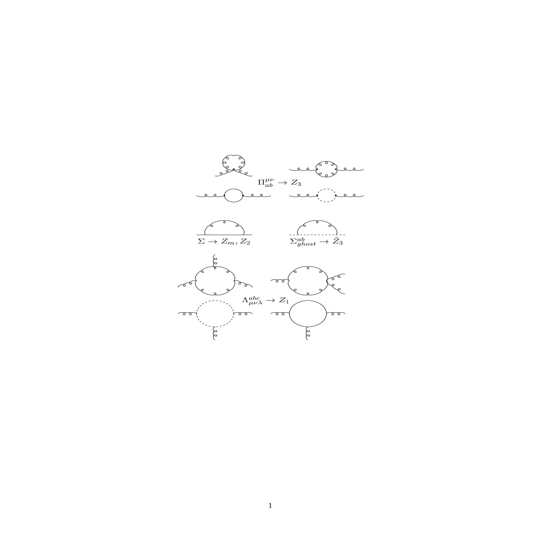
The quark self energy $\Sigma(p)$ is similar to the electron self energy apart from a group theoretical factor. $\Sigma(p)$ has been calculated in PRD3 within IR. It reads

$$\Sigma(p) = -ig^{2}C_{2}(r)(p/-4m)I_{\log}(m^{2})+g^{2}g^{\mu\nu}\Upsilon_{\mu\nu}^{(0)}p/$$ (35)

$$+ (Z_{2}-1)p/-(Z_{2}Z_{m}-1)m+\widetilde{\Sigma}(p,m)\,,$$

where the tilde means that the quantity is finite. We shall use such notation from now on. Indeed $\widetilde{\Sigma}(p,m)$ is both ultraviolet and infrared finite. In order to define the corresponding renormalization constants we consistently make use of (9) in order to pursuit a mass independent scheme as well as introducing the arbitrary constant $\lambda^{2}$. It is noteworthy that the $b\ln\mu^{2}$ piece coming from (9) cancels exactly the infrared divergence in the ultraviolet finite portion of the amplitude, as it should.

Henceforth we shall systematically define the renormalization constants in a mass independent fashion (which defines the “minimal” scheme in IR) as well as set $\alpha_{i}$’s ($\Upsilon$’s) to zero. We define this procedure as constrained IR (CIR). We shall no longer write the $\Upsilon$’s explicitly in the remaining amplitudes for the sake of brevity.

Therefore the fermion mass and field renormalization constants can be cast as

$$Z_{m} = 1+3iC_{2}(r)I_{\log}(\lambda^{2})g^{2}+O(g^{3})\,,$$

$$Z_{2} = 1+iC_{2}(r)I_{\log}(\lambda^{2})g^{2}+O(g^{3})\,.$$ (36)

After the appropriate color index contractions, the one loop correction for the ghost propagator simplifies to

$$\Sigma_{ghost}^{ab}(p^{2}) = g^{2}g_{\mu\nu}C_{2}(G)\delta^{ab}\int_{k}\frac{(p-k)^{\mu}p^{\nu}}{[(p-k)^{2}-\mu^{2}](k^{2}-\mu^{2})}$$ (37)

$$+ ({\tilde{Z_{3}}}-1)\delta^{ab}p^{2}\,,$$

where $\mu^{2}$ is an infrared mass regulator for both the ghost and gluon propagators. After some straightforward algebra we have

$$\Sigma_{ghost}^{ab}(p^{2},\lambda^{2}) = \delta^{ab}p^{2}\Big{(}\frac{ig^{2}}{2}C_{2}(G)I_{\log}(\lambda^{2})$$ (38)

$$+ {\tilde{Z_{3}}}-1\Big{)}+\widetilde{\Sigma}^{ab}_{ghost}(p^{2},\lambda^{2})\,,$$

from which we define the renormalization constant

$$\tilde{Z}_{3}=1-\frac{i}{2}C_{2}(G)I_{\log}(\lambda^{2})g^{2}+O(g^{3}).$$ (39)

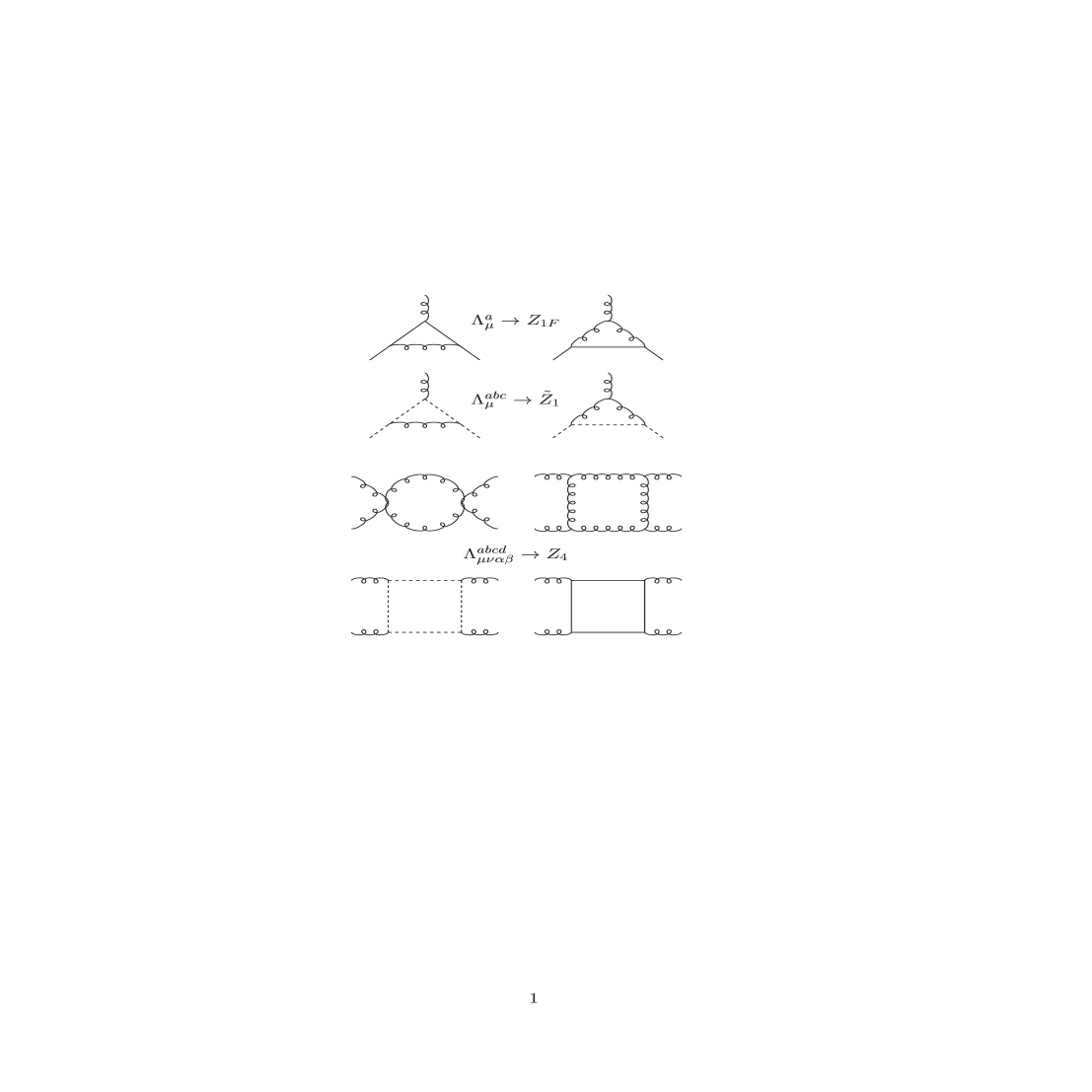
For the one loop quark-gluon vertex $\Lambda^{a}_{\mu}$ shown in fig. (2) we have two contributions: the QED-like electron-photon vertex diagram $\Lambda^{a}_{\mu}(p,q)(1)$ and the one involving the three-gluon vertex $\Lambda^{a}_{\mu}(p,q)(2)$. The former differs from the QED electron-photon vertex by a group theoretical factor

$$\Lambda^{a}_{\mu}(p,q)(1)=(t^{d}t^{a}t^{d})\Lambda_{\mu}^{QED}(p,q)\,.$$ (40)

We have also computed $\Lambda_{\mu}^{QED}(p,q)$ within IR in PRD3 so here we only quote the result:

$$i\Lambda_{\mu}^{QED}(p,q)=\gamma^{\mu}[\alpha_{2}+I_{log}(m^{2})]+\tilde{\Lambda}^{\mu}(p,q)\,,$$ (41)

where $m$ is the mass of the fermion, $\tilde{\Lambda}^{\mu}(p,q)$ is finite and $\alpha_{2}$ is arbitrary and shall be set to zero within constrained IR. Using that $t^{d}t^{a}t^{d}=[C_{2}(r)-1/2\,C_{2}(G)]t^{a}$ enables us to write

$$\Lambda^{a}_{\mu}(p,q,\lambda^{2})(1)=-ig^{3}t^{a}\gamma_{\mu}\Big{(}C_{2}(r)-\frac{1}{2}C_{2}(G)\Big{)}\times$$

$$\times\Big{(}I_{log}(\lambda^{2})+\tilde{\Lambda}^{a}(p,q,\lambda^{2})(1)\Big{)}\,.$$ (42)

As for $\Lambda^{a}_{\mu}(p,q)(2)$, the Feynman rules give

$$i\Lambda^{a}_{\mu}(p,q)(2)=g^{3}f^{abc}t^{b}t^{c}\int_{k}\frac{{\cal{}_{N}}_{\mu}}{{\cal{D}}}$$ (43)

with

$${\cal{N}}_{\rho} = \gamma^{\mu}(k/+m)\gamma^{\nu}\Big{(}(2p-q-k)_{\nu}g_{\mu\rho}$$

$$+ (2k-p-q)_{\rho}g_{\mu\nu}+(2q-p-k)_{\mu}g_{\nu\rho}\Big{)}\,,$$

$${\cal{D}} = (k^{2}-m^{2})[(k-p)^{2}-\mu^{2}][(k-q)^{2}-\mu^{2}]\,.$$ (44)

where again $\mu$ is a mass regulator for the gluon propagator. We proceed as before. We remove the external momentum dependence from the ILI by applying the identity (1) in the propagators which contain the momenta $p$ and $q$ above. Then we isolate a genuine (ultraviolet divergent only) contribution for the counterterm with the help of identity (9) to get, in CIR,

$$\Lambda^{a}_{\mu}(p,q,\lambda^{2})(2) = -i\frac{3}{2}g^{3}C_{2}(G)t^{a}\Big{(}\gamma_{\mu}I_{log}(\lambda^{2})$$ (45)

$$+ \tilde{\Lambda}^{a}_{\mu}(p,q,\lambda^{2})(2)\Big{)}\,.$$

Finally we define the renormalization constant $Z_{1F}$ to one loop order by adding up the two contributions for the quark-gluon vertex:

$$\Lambda^{a}_{\mu}(p,q,\lambda^{2}) = g\gamma_{\mu}t^{a}\Big{(}-ig^{2}(C_{2}(G)+C_{2}(r))I_{log}(\lambda^{2})+$$ (46)

$$+ Z_{1F}-1+\widetilde{\Lambda}^{a}(p,q,\lambda^{2})\Big{)}$$

which gives

$$Z_{1F}=1+ig^{2}\Big{(}C_{2}(G)+C_{2}(r)\Big{)}I_{log}(\lambda^{2})\,.$$ (47)

To calculate the renormalization constant $\tilde{Z}_{1}$ we work with the ghost-gluon vertex. It receives two contributions (fig. 2): the ghost-ghost-gluon loop ${\Lambda}^{abc}_{1\mu}$ and the ghost-gluon-gluon loop ${\Lambda}^{abc}_{2\mu}$. Let $p_{1}$, $p_{2}$ and $p_{1}+p_{2}\equiv q$ be the external momenta. Thus

$${\Lambda}^{abc}_{\mu}=\tilde{\Lambda}^{abc}_{1\mu}+{\Lambda}^{abc}_{2\mu}+(-i)gf^{abc}q_{\mu}({\tilde{Z_{1}}}-1)\,.$$ (48)

It is straightforward to use the Feynman rules with the help of the identity $f^{afe}f^{bep}f^{cpf}=N/2f^{abc}$ for $SU(N)$ to get

$${\Lambda}^{abc}_{1\mu}(p_{1},p_{2})=-\frac{g^{3}}{2}C_{2}(G)f^{abc}q^{\alpha}$$

$$\int_{k}\frac{k_{\alpha}k_{\mu}}{(k^{2}-\mu^{2})[(k-p_{1})^{2}-\mu^{2}][(k-q)^{2}-\mu^{2}]}\,.$$ (49)

We proceed according to the rules of CIR, as we have done before, to arrive at

$${\Lambda}^{abc}_{1\mu}(p_{1},p_{2})=\frac{g^{3}}{8}C_{2}(G)f^{abc}q_{\mu}I_{log}(\lambda^{2})+\tilde{{\Lambda}}^{abc}_{1\mu}(p_{1},p_{2})\,.$$ (50)

Similarly we have for the other contribution

$${\Lambda}^{abc}_{2\mu}(p_{1},p_{2})=\frac{3g^{3}}{8}C_{2}(G)f^{abc}q_{\mu}I_{log}(\lambda^{2})+\tilde{{\Lambda}}^{abc}_{2\mu}(p_{1},p_{2})\,,$$ (51)

and hence

$${\Lambda}^{abc}_{\mu}(p_{1},p_{2}) = -igf^{abc}q_{\mu}\Big{(}-i\frac{g^{2}}{2}C_{2}(G)I_{log}(\lambda^{2})+\tilde{Z}_{1}-1\Big{)}$$ (52)

$$+ \tilde{{\Lambda}}^{abc}_{\mu}(p_{1},p_{2})\,.$$

Finally we define the renormalization constant in a minimal fashion within IR as

$$\tilde{Z}_{1}=1+\frac{i}{2}g^{2}C_{2}(G)I_{log}(\lambda^{2})\,.$$ (53)

The class of one loop three-gluon vertex graphs from which we shall define $Z_{1}$ are shown in fig. 1. They have been explicitly computed in Celmaster , Pascual within DR. The calculation is straightforward yet tedious. We have proceeded according to the rules of CIR as before in order to isolate the ultraviolet divergence as a term proportional to $I_{log}(\lambda^{2})$ after making use of (9). The infrared divergent piece proportional to $\ln(\lambda^{2}/\mu^{2})$ as $\mu\rightarrow 0$ cancels out with an alike term stemming from the ultraviolet finite piece of the amplitude as we generically discuss in the appendix B. For the sake of brevity we shall present only the result here. Let $p$ and $q$ be the external momenta. Then

$$\Lambda^{abc}_{\mu\nu\lambda}(p,q) = -igf^{abc}V_{\mu\nu\lambda}(p,q,p+q)\times$$ (54)

$$\times \Bigg{(}-ig^{2}\Big{(}-\frac{2}{3}C_{2}(G)+\frac{4}{3}C(r)n_{f}\Big{)}I_{log}(\lambda^{2})$$

$$+ Z_{1}-1\Bigg{)}+\widetilde{\Lambda}^{abc}_{\mu\nu\lambda}(p,q)\,,$$

$V_{\mu\nu\lambda}(p,q,p+q)=(p-q)_{\lambda}g_{\mu\nu}-p_{\mu}g_{\nu\lambda}+q_{\nu}g_{\mu\lambda}$, from which we define

$$Z_{1}=1+ig^{2}\Bigg{(}-\frac{2}{3}C_{2}(G)+\frac{4}{3}C(r)n_{f}\Bigg{)}I_{log}(\lambda^{2})\,.$$ (55)

Last but not least we have to compute the four gluon vertices depicted in fig. 2 along with all their permutations. This long calculation has been performed with great detail by Pascual and Tarrach in Pascual in the Weinberg’s scheme as well as by Papavassiliou in Papavassiliou using the S-matrix pinch technique . The corresponding result within CIR reads:

$$\Lambda^{abcd}_{\alpha\beta\mu\nu}(p_{1},p_{2},p_{3},p_{4})=-g^{2}W^{abcd}_{\alpha\beta\mu\nu}\times$$

$$\times\Bigg{(}-\frac{ig^{2}}{3}\Big{(}C_{2}(G)+4C(r)n_{f}\Big{)}I_{log}(\lambda^{2})+Z_{4}-1\Bigg{)}$$

$$+\,\widetilde{\Lambda}^{abcd}_{\alpha\beta\mu\nu}(p_{1},p_{2},p_{3},p_{4})\,,$$ (56)

where we have used the same notation as T. Muta Muta , namely

$$W^{a_{1}a_{2}a_{3}a_{4}}_{\mu_{1}\mu_{2}\mu_{3}\mu_{4}} = (f^{13,24}-f^{14,32})g_{\mu_{1}\mu_{2}}g_{\mu_{3}\mu_{4}}$$ (57)

$$+ (f^{12,34}-f^{14,23})g_{\mu_{1}\mu_{3}}g_{\mu_{2}\mu_{4}}$$

$$+ (f^{13,42}-f^{12,34})g_{\mu_{1}\mu_{4}}g_{\mu_{3}\mu_{2}}\,,$$

with $f^{ij,lm}=f^{a_{i}a_{j}a}f^{aa_{l}a_{m}}$. Therefore

$$Z_{4}=1+ig^{2}\Bigg{(}\frac{1}{3}C_{2}(G)+\frac{4}{3}C(r)n_{f}\Bigg{)}I_{log}(\lambda^{2})\,.$$ (58)

III Slavnov-Taylor Identities and Renormalization Group Functions

It is a simple task to verify that CIR explicitly preserves the Slavnov-Taylor identities expressed by (15):

$$\frac{Z_{1}}{Z_{3}}=\frac{\tilde{Z}_{1}}{\tilde{Z}_{3}}=\frac{Z_{1F}}{Z_{2}}=\frac{Z_{4}}{Z_{1}}=1+ig^{2}C_{2}(G)I_{log}(\lambda^{2})\,.$$ (59)

In other words CIR explicitly fixes the arbitrariness of IR in such a way that gauge invariance is maintained. At higher loop order similar relations to those displayed in equations (4)-(7) are expected to hold JHEP and its constrained version should implement vector gauge invariance as well WIP .

In defining a mass-independent minimal scheme in CIR there appeared an arbitrary non-vanishing constant $\lambda^{2}$. As discussed before, by subtracting only the term proportional to $I_{log}(\lambda^{2})$ defines a minimal subtraction scheme within IR and we are left with the finite piece of the amplitude which is also dependent upon $\lambda^{2}$. Moreover it is identical to the amplitude that we would obtain had we employed differential renormalization PRD3 , DiffR . The arbitrary scales which appear in IR and Differential renormalization can be identified and thus the truncated connected $n$-point renormalized Green’s function, say $G^{(n)}_{c}(p_{i},g,m)$ is expected to satisfy a Callan-Symanzik like renormalization group equation where $\lambda$ plays the role of renormalization group scale. Thus we have

$$\Bigg{(}\lambda\frac{\partial}{\partial\lambda}+\beta(g)\frac{\partial}{\partial g}-\gamma_{m}(g)m\frac{\partial}{\partial m}$$

$$-n_{A}\gamma_{A}(g)-n_{f}\gamma_{\psi}(g)\Bigg{)}G^{(n)}_{c}=0\,,$$ (60)

where $n_{A}$ ($n_{f}$) is the number of gluon (quark) legs in momentum space, $m$ and $g$ are defined as in (13), $\gamma_{A}(\gamma_{\psi})$ are the anomalous dimension of the gluon (quark) field and

$$\beta(g) = \lambda\frac{\partial g}{\partial\lambda}\,,$$

$$\gamma_{m}(g) = -\frac{\lambda}{m}\frac{\partial m}{\partial\lambda}\,,$$

$$\gamma_{A}(g) = \frac{\lambda}{2Z_{3}}\frac{\partial Z_{3}}{\partial\lambda}\,\,\,\mbox{and}$$

$$\gamma_{\psi}(g) = \frac{\lambda}{2Z_{2}}\frac{\partial Z_{2}}{\partial\lambda}\,.$$ (61)

For instance let us explicitly calculate the $\beta$ function. Recall (13): $g_{0}=Z_{g}g$, $Z_{g}=Z_{1}Z_{3}^{-3/2}$. Hence

$$2\lambda^{2}\frac{\partial}{\partial\lambda^{2}}\Big{(}Z_{g}g\Big{)}=0\,.$$ (62)

Now using that

$$\lambda^{2}\frac{\partial}{\partial\lambda^{2}}I_{log}(\lambda^{2})=-b$$ (63)

in the equation above yields after some simple algebra

$$\beta=-\frac{g^{3}}{3(4\pi)^{2}}\Big{(}11C_{2}(G)-4C(r)n_{f}\Big{)}+O(g^{5})\,.$$ (64)

In a similar fashion we may use the renormalization constants which we have calculated in CIR to show that

$$\gamma_{m}=\frac{6g^{2}}{(4\pi)^{2}}C_{2}(r)+O(g^{5})\,,$$ (65)

$$\gamma_{A}=-\frac{g^{2}}{3(4\pi)^{2}}\Big{(}5C_{2}(G)-4C(r)n_{f}\Big{)}+O(g^{5})\,,$$ (66)

and

$$\gamma_{\psi}=\frac{g^{2}}{(4\pi)^{2}}C_{2}(r)+O(g^{5})\,,$$ (67)

which are the standard values of the renormalization group functions. Particularly in a minimal scheme within our framework, they coincide with the MS scheme in dimensional regularization.

IV Conclusions

We have applied the IR method to QCD at the one loop level. We have shown that it preserves non abelian gauge symmetry and that there is no need of a different prescription to deal with massive or massless theories. A constrained version of IR which implies in momentum routing invariance also delivers gauge invariant amplitudes for the non-abelian case.

Appendix A:

Consider a bubble (or a piece of a certain QCD amplitude) :

$$I^{d} = \Lambda^{4-d}\int_{k}^{d}\frac{1}{(k^{2}-\mu^{2})[(k+p)^{2}-\mu^{2}]}.$$ (68)

The index $d$ stands for dimensional regularization. Although IR does not use a explicit regulator, we will use dimensional regularization here for pedagogical purposes to show how to define a irreducible loop integral in a massless theory free of infrared divergencies through equation (9). Similar relations can be derived at higher loop order JHEP .

We follow the prescription of IR to separate the divergent parts by means of the identity given by equation (1). As we have discussed we may strictly assume an implicit regulator to manipulate algebraically the integrand. However as we do not actually evaluate the irreducible loop integrals we need not to make a regulator explicit.

$$I^{d} = \Lambda^{2\epsilon}\left\{\int_{k}\frac{1}{(k^{2}-\mu^{2})^{2}}\right.$$ (69)

$$- \left.\int_{k}\frac{p^{2}+2p\cdot k}{(k^{2}-\mu^{2})^{2}[(k+p)^{2}-\mu^{2}]}\right\},$$

with $\epsilon=2-d/2$. As a matter of illustration we calculate the first integral ($I_{log}(m^{2})$) using dimensional regularization to obtain

$$\Lambda^{2\epsilon}I_{log}(m^{2})=b\left[\frac{1}{\epsilon}+A+\ln{\left(-\frac{4\Lambda^{2}}{m^{2}}\right)}\right]+{\cal O}(\epsilon),$$ (70)

where $A$ is a constant characteristic of dimensional regularization. The second integral is finite and evaluates to

$$I^{d}_{fin}=-b\int_{0}^{1}\mbox{dz}\ln{\left(\frac{p^{2}z(1-z)-\mu^{2}}{-\mu^{2}}\right)}.$$ (71)

In the limit where $\mu^{2}\to 0$, we have

$$I^{d}_{fin}=-b\ln{\left(-\frac{p^{2}}{e^{2}\mu^{2}}\right)}.$$ (72)

In IR we write

$$I^{d}=I_{log}(\mu^{2})-b\ln{\left(-\frac{p^{2}}{e^{2}\mu^{2}}\right)}.$$ (73)

However because

$$\Lambda^{2\epsilon}I_{log}(\lambda^{2})=b\left[\frac{1}{\epsilon}+A+\ln{\left(-\frac{4\Lambda^{2}}{\lambda^{2}}\right)}\right]+{\cal O}(\epsilon),$$ (74)

$\lambda\neq 0$ we have

$$\Lambda^{2\epsilon}I_{log}(\mu^{2})-\Lambda^{2\epsilon}I_{log}(\lambda^{2})=b\ln{\left(\frac{\lambda^{2}}{\mu^{2}}\right)}.$$ (75)

which is just equation (9) in the limit $\epsilon\rightarrow 0$. Substituting this relation in the expression for $I^{d}$ yields

$$I^{d}=I_{log}(\lambda^{2})-b\ln{\left(\frac{p^{2}}{e^{2}\lambda^{2}}\right)}.$$ (76)

Now we are allowed to subtract a genuine ultraviolet divergent object $I_{log}(\lambda^{2})$ by defining the appropriate counterterm. The non-vanishing arbitrary parameter $\lambda$ plays the role of renormalization group scale.

Appendix B: Infrared Finiteness of the One-Loop Amplitudes

We now turn ourselves to an important discussion on a problem which arises when the limit $\mu^{2}\to 0$ is taken. We must make sure that, when using the scale relation given by equation (7), the term in $\ln{(\mu^{2}/\lambda^{2})}$ will be cancelled out by a contribution that comes from the ultraviolet finite part. The divergent integrals that are present in the calculations at the one loop level for the renormalization of QCD are

$$A = \int_{k}\frac{1}{(k^{2}-\mu^{2})[(k+p)^{2}-\mu^{2}]};$$ (77)

$$A_{\mu} = \int_{k}\frac{k_{\mu}}{(k^{2}-\mu^{2})[(k+p)^{2}-\mu^{2}]};$$ (78)

$$B_{\mu\nu} = \int_{k}\frac{k_{\mu}k_{\nu}}{(k^{2}-\mu^{2})[(k+p)^{2}-\mu^{2}][(k+q)^{2}-\mu^{2}]}$$ (79)

$$B_{\mu\nu\alpha} = \int_{k}\frac{k_{\mu}k_{\nu}k_{\alpha}}{(k^{2}-\mu^{2})[(k+p)^{2}-\mu^{2}][(k+q)^{2}-\mu^{2}]}.$$ (80)

In the integrals above we have introduced the mass $\mu$, that will be set to zero in the end. Since the integrals are assumed to be regularized, we can follow the prescription of Implicit Regularization, and separate the divergent parts by means of the identity given by equation (1). Below we show the calculations:

• $A$:

  $$A = \int_{k}\frac{1}{(k^{2}-\mu^{2})^{2}}$$ (81)

  $$- \int_{k}\frac{p^{2}+2p\cdot k}{(k^{2}-\mu^{2})^{2}[(k+p)^{2}-\mu^{2}]}.$$

  We now use the identity expressed by equation (7) in the first integral. The second one, which is finite and does not depend on any specific technique, is given by

  $$A_{fin}=b\int_{0}^{1}\mbox{dz}\ln{\left(\frac{p^{2}z(1-z)-\mu^{2}}{-\mu^{2}}\right)}.$$ (82)

  For $\mu^{2}\to 0$, we have

  $$A_{fin}=b\ln{\left(-\frac{p^{2}}{e^{2}\mu^{2}}\right)}.$$ (83)

  We clearly see that the $\mu^{2}$ cancels out when the two parts are put together, so that we obtain

  $$A=I_{log}(\lambda^{2})-b\ln{\left(-\frac{p^{2}}{e^{2}\lambda^{2}}\right)}.$$ (84)

• $A_{\mu}$: After the expansion, some integrals vanish, since their integrands are odd in the integration variable. After calculating the finite part, we have

  $$A_{\mu}=-2p^{\nu}\int\frac{k_{\mu}k_{\nu}}{(k^{2}-\mu^{2})^{3}}+\frac{b}{2}p_{\mu}\ln{\left(-\frac{p^{2}}{e^{2}\mu^{2}}\right)}.$$ (85)

  The divergent integral is $\Theta^{(0)}_{\mu\nu}(\mu^{2})$ (see eq. (6)) and we use equation (3) to write

  $$\Theta^{(0)}_{\mu\nu}(\mu^{2}) = \frac{g_{\mu\nu}}{4}\left(I_{log}(\mu^{2})-\alpha_{2}\right)$$ (86)

  $$= \frac{g_{\mu\nu}}{4}\left(I_{log}(\lambda^{2})+b\ln{\left(\frac{\lambda^{2}}{\mu^{2}}\right)}-\alpha_{2}\right)$$

  Again we see the cancellation of $\mu^{2}$ when the finite part is considered. We are left with

  $$A_{\mu}=-\frac{p_{\mu}}{2}\left(I_{log}(\lambda^{2})-b\ln{\left(-\frac{p^{2}}{e^{2}\lambda^{2}}\right)}-\alpha_{2}\right).$$ (87)

  It is important to note that equation (3) is essential in the cancelation of the $\mu^{2}$.

• $B_{\mu\nu}$: After the expansion and calculation of the finite part, we obtain

  $$B_{\mu\nu} = \int_{k}\frac{k_{\mu}k_{\nu}}{(k^{2}-\mu^{2})^{3}}-b\frac{g_{\mu\nu}}{4}\ln{\left(-\frac{p^{2}}{e^{2}\mu^{2}}\right)}$$ (88)

  $$+ b\left\{\left[\left(\frac{1}{2}+\mu^{2}\eta_{00}\right)-\frac{q^{2}}{2}\eta_{10}-\frac{p^{2}}{2}\eta_{01}\right]\right.$$

  $$+ \left.p_{\mu}p_{\nu}\eta_{02}+q_{\mu}q_{\nu}\eta_{20}+(p_{\mu}q_{\nu}+q_{\mu}p_{\nu})\eta_{11}\right\},$$

  where

  $$\eta_{nm}=\int_{0}^{1}\mbox{dz}\int_{0}^{1-z}\mbox{dy}\frac{z^{n}y^{m}}{Q(p,q,y,z)}$$ (89)

  and

  $$Q(p,q,y,z) = p^{2}y(1-y)+q^{2}z(1-z)$$ (90)

  $$- 2(p\cdot q)yz-\mu^{2}.$$

  It can be easily seen that the functions $\eta_{nm}$ do not have problems when $\mu^{2}\to 0$. The divergent integral has the result of equation (86), so that

  $$B_{\mu\nu} = \frac{g_{\mu\nu}}{4}\left(I_{log}(\lambda^{2})-b\ln{\left(-\frac{p^{2}}{e^{2}\lambda^{2}}\right)}-\alpha_{2}\right)$$ (91)

  $$+ f(\eta_{nm}),$$

  where $f(\eta_{nm})$ represents the $\eta$ dependent part.

• $B_{\mu\nu\alpha}$: The mechanism is the same as in the other integrals:

  $$B_{\mu\nu\alpha} = -2(p+q)^{\beta}\int_{k}\frac{k_{\mu}k_{\nu}k_{\alpha}k_{\beta}}{(k^{2}-\mu^{2})^{4}}$$ (92)

  $$+ \frac{b}{12}\left[(p+q)_{\mu}g_{\nu\alpha}+(p+q)_{\nu}g_{\mu\alpha}\right.$$

  $$+ \left.(p+q)_{\alpha}g_{\mu\nu}\right]\ln{\left(-\frac{p^{2}}{e^{2}\mu^{2}}\right)}+g(\eta_{nm}).$$

  The $g(\eta)$ represents the $\eta$ dependent part. The divergent integral is $\Theta^{(0)}_{\mu\nu\alpha\beta}(\mu^{2})$, as defined in equation (6). We use the relation given by equation (5) to write

  $$\Theta^{(0)}_{\mu\nu\alpha\beta}(\mu^{2}) = \frac{1}{24}g_{\{\mu\nu}g_{\alpha\beta\}}\left(I_{log}(\mu^{2})-\alpha_{4}\right)$$ (93)

  $$= \frac{1}{24}g_{\{\mu\nu}g_{\alpha\beta\}}\left(I_{log}(\lambda^{2})\right.$$

  $$+ \left.b\ln{\left(\frac{\lambda^{2}}{\mu^{2}}\right)}-\alpha_{4}\right).$$

  The substitution of this result in $B_{\mu\nu\alpha}$ and the adoption of the same procedures as before, lead us to the cancellation of the infrared divergences and we have the final expression

  $$B_{\mu\nu\alpha} = -\frac{1}{12}\left[(p+q)_{\mu}g_{\nu\alpha}+(p+q)_{\nu}g_{\mu\alpha}\right.$$ (94)

  $$+ \left.(p+q)_{\alpha}g_{\mu\nu}\right]\left(I_{log}(\lambda^{2})\right.$$

  $$- \left.b\ln{\left(-\frac{p^{2}}{e^{2}\mu^{2}}\right)}-\alpha_{4}\right)+g(\eta_{nm}).$$

We call the reader’s attention to the fact that, in the last calculation, the equation (5) was mandatory in order to $\mu^{2}$ to be cancelled. It is also interesting to note that the same relations that are necessary to preserve gauge invariance are also essential for the cancellation of the infrared cut-off $\mu^{2}$.

References

- (1) W. Siegel, Phys. Lett. B84 (1979) 153; idem Phys. Lett. B94 (1980) 37.
- (2) I. Jack and D. R. T. Jones, hep-ph/9707278 in “Perspectives on Supersymmetry ”, World Scientific, Ed. G. Kane, 1997.
- (3) D. Carneiro, A. P. Baêta Scarpelli, Marcos Sampaio and M. C. Nemes, JHEP 0312 (2003) 044.
- (4) R. Jackiw, Int. J. Mod. Phys. B14 (2000) 2011.
- (5) R. Jackiw in Current Algebra and Anomalies, S. Treiman, R. Jackiw, B. Zumino and E. Witten eds., Princeton Univ. Press, World Scientific, Singapore (1985).
- (6) A. P. Baêta Scarpelli, Marcos Sampaio and M. C. Nemes, Phys. Rev. D63 (2001) 046004.
- (7) A. P. Baêta Scarpelli, Marcos Sampaio, B. Hiller and M. C. Nemes, Phys. Rev. D64 (2001) 046013.
- (8) Marcos Sampaio, A. P. Baêta Scarpelli, B. Hiller, A. Brizola, M. C. Nemes and S. Gobira, Phys. Rev. D65 (2002) 125023.
- (9) O. A. Battistel and M. C. Nemes, Phys. Rev. D59 (1999) 055010.
- (10) S. Gobira and M. C. Nemes, Int. J. Theor. Phys. 42 (2003) 2765.
- (11) T. Muta, Foundations of Quantum Chromodynamics, World Scientific Lecture Notes in Physics - Vol. 5 (1987).
- (12) A. L. Mota, B. Hiller, Marcos Sampaio, M. C. Nemes and A. A. Osipov, A Renormalizable Nambu and Jona-Lasinio-like SU(3) Model and Hadronic Properties of Light Mesons, Work in progress.
- (13) T. Gherghetta, Phys. Rev. D50 (1994) 5985.
- (14) Y. L. Wu, Phys. Rev. D64 (2001) 016001.
- (15) G. Dunne, Phys. Lett. B293 (1992) 367.
- (16) W. Celmaster and R. J. Gonsalves, Phys. Rev. D20 (1979) 1420.
- (17) P. Pascual and R. Tarrach, Nucl. Phys. B174 (1980) 123.
- (18) J. Papavassiliou, Phys. Rev. D47 (1993) 4728.
- (19) D. Z. Freedman, K. Johnson and J. I. Latorre, Nucl. Phys. B371 (1992) 353; P. E. Haagensen, J. I. Latorre, Ann. Phys. 221 (1993) 77; idem Phys. Lett. B283 (1992) 293; M. Chaichian, W. F. Chen, Phys. Lett. B409 (1997) 325; M. Pérez-Victoria, Phys. Lett. B442 (1998) 315; F. del Águila, A. Culatti, R. Muñoz Tapia, M. Pérez-Victória, Nucl. Phys. B537 (1999) 561; idem Nucl. Phys. B504 (1997) 532.
- (20) Marcos Sampaio, M. C. Nemes and A. P. Baêta Scarpelli, Work in Progress.