Renormalization–Group Analysis
of Layered Sine–Gordon Type Models

Abstract

We analyze the phase structure and the renormalization group (RG) flow of the generalized sine-Gordon models with nonvanishing mass terms, using the Wegner-Houghton RG method in the local potential approximation. Particular emphasis is laid upon the layered sine-Gordon (LSG) model, which is the bosonized version of the multi-flavour Schwinger model and approaches the sum of two “normal”, massless sine-Gordon (SG) models in the limit of a vanishing interlayer coupling $J$. Another model of interest is the massive sine-Gordon (MSG) model. The leading-order approximation to the UV (ultra-violet) RG flow predicts two phases for the LSG as well as for the MSG, just as it would be expected for the SG model, where the two phases are known to be separated by the Coleman fixed point. The presence of finite mass terms (for the LSG and the MSG) leads to corrections to the UV RG flow, which are naturally identified as the “mass corrections”. The leading-order mass corrections are shown to have the following consequences: (i) for the MSG model, only one phase persists, and (ii) for the LSG model, the transition temperature is modified. Within the mass-corrected UV scaling laws, the limit of $J\to 0$ is thus nonuniform with respect to the phase structure of the model. The modified phase structure of general massive sine-Gordon models is connected with the breaking of symmetries in the internal space spanned by the field variables. For the LSG, the second-order subleading mass corrections suggest that there exists a cross-over regime before the IR scaling sets in, and the nonlinear terms show explicitly that higher-order Fourier modes appear in the periodic blocked potential.

1 Introduction

At the heart of every quantum field theory, there is the need for renormalization. In the framework of the well-known perturbative renormalization procedure (see e.g. [1, 2]), the potentials—or interaction Lagrangians—are decomposed in a Taylor series in the fields; this Taylor series generates the vertices of the theory. If the expansion contains only a finite number of terms (this is the “normal” case), then each interaction vertex can be treated independently. However, certain theories exist which cannot be considered in this traditional way. In some theories, symmetries of the Lagrangian impose the requirement of taking infinitely many interaction vertices into account; any truncation of these infinite series would lead to an unacceptable violation of essential symmetries of the model. The subject of this article is to consider theories which fall into the latter category.

Specifically, we here consider generalizations of the well-known sine-Gordon (SG) scalar field theory with mass terms. The “pure,” massless SG model is periodic in the internal space spanned by the field variable. One of the central subjects of investigation is the layered sine-Gordon (LSG) model [4, 3], where the periodicity is broken by a coupling term between two layers each of which is described by a scalar field. All generalizations of the SG model discussed here belong to a wider class of massive sine-Gordon type models for two coupled Lorentz-scalar fields, which form an $O(2)$ “flavour” doublet, i.e. which are invariant under a global rotation in the internal space of the field variables, though not necessarily periodic. All Lagrangians investigated here contain self-interaction terms which are periodic in the field variables, but this periodicity is broken by the mass terms.

Regarding the phase structure, it is known that the massless sine-Gordon (SG) model for scalar, flavour singlet together with the two-dimensional XY model and Coulomb gas belong to the same universality class. For the two-dimensional Coulomb gas, the absence of long-range order, the existence of the Coleman fixed point and the presence of a topological (Kosterlitz–Thouless) phase transition have been proven rigorously in Refs. [5, 6, 7, 8, 9, 10]. It was shown that the dimensionful effective potential becomes a field-independent constant in both phases of the SG model [10].

The joint feature of the massless and massive SG models is the presence of a self-interaction potential which is periodic in the various directions of the internal space. This makes it necessary to treat these models in a manner which avoids the Taylor-expansion of the periodic part of the potential. Hence, the renormalization [14, 11, 12, 13] of these models cannot be considered in the framework of the usual perturbative expansion [1, 2]. The massive SG models open a platform to investigate the effect of a broken periodicity in the internal space. For the flavour singlet field, periodicity is broken entirely by a mass term, and the ground state is characterized by a vanishing field configuration [15].

For the flavour doublet, one possible way to realize a partial breaking of periodicity is given by a single nonvanishing mass eigenvalue. Alternatively, two eigenvalues of the “mass matrix” that enters the Lagrangian may be nonzero. We here investigate the effect of entire and partial breaking of periodicity in the internal space on the ultraviolet (UV) scaling laws and on the existence of the Coleman fixed point. We shall restrict ourselves to various approximations of the RG flow equation for the blocked potential.

The LSG model, because of its layered structure, has a connection to solid-state physics. In particular, it has been used to describe the vortex properties of high transition-temperature superconductors (HTSC) [16, 17, 18, 19, 20]. The real-space renormalization group (RG) analysis of the LSG model, invariably based on the dilute vortex gas approximation, has been successfully applied for the explanation of electric transport properties of HTSC materials [16, 18, 20, 21]. New experimental data are in disagreement with theoretical predictions, and this aspect may require a more refined analysis as compared to the dilute gas approximation [22, 21].

There exist connections of the generalized sine-Gordon models to fundamental questions of field theory. For instance, a special case of the massive SG-type models is just the bosonized version of the massive Schwinger model, which in turn is an exactly solvable two-dimensional toy-model of strong confining forces [3, 4]. The flavour singlet field can then be considered a meson field with vanishing flavour charge (“baryon number”), while the flavour doublet field models “baryons” with “baryon charge” $\pm\frac{1}{2}$. Here, we restrict ourselves to the investigation of the vacuum sector with zero total flavour charge (“baryon charge”) [23, 24]. Of fundamental importance is the following question: Are there any operators, irrelevant in the bare theory, which become relevant for the infrared (IR) physics? Our investigations hint at some interesting phenomena which are connected with cross-over regions in which UV-irrelevant couplings may turn into IR-relevant operators, after passing through intermediate scales. The IR-relevant “confining forces” would correspond to the interactions among the “hadrons” in our language. In the case of QCD, the much more serious problem of the determination of the operators relevant for confinement (i.e., for building up the hadrons) may, in principle, carry some similarities to the model problems studied here.

Our paper is organized as follows. In Sec. 2, we give a short overview of all classes of massive generalized sine-Gordon models, of the flavour-doublet type, which are relevant for the current investigation, including the LSG and the MSG models. Section 3 includes the basic relations used for the Wegner-Houghton (WH) RG method [25] in the local potential approximation. In Sec. 4, we start with the outline of various approximations to the WH–RG used in the present paper. The UV scaling laws for the massless and massive models are found analytically in subsections 4.2 and 4.3, respectively. In subsection 4.3, the existence of the Coleman fixed point in massive SG models is also discussed on the basis of the UV scaling laws for various special cases, with entire and partial breaking of periodicity, for flavour-doublet and flavour-singlet fields. In Sec. 4.4, the UV scaling laws are enhanced by keeping the subleading nonlinear terms in the mass-corrected RG flow equation for the blocked potential. In this approximation, the numerical determination of the RG flow is presented for the LSG model, and the existence of a cross-over region from the UV to the IR scaling regimes is demonstrated to persist after the inclusion of the subleading terms. Finally, the main results are summarized in Sec. 5.

2 Two-flavour Massive sine-Gordon Model

In this article, we investigate a class of Euclidean scalar models for the flavour $O(2)$-doublet

$${\underline{\varphi}}=\begin{pmatrix}\varphi_{1}\cr\varphi_{2}\end{pmatrix}$$ (1)

in $d=2$ spatial dimensions. The bare Lagrangians are assumed to have the following properties:

1. The Lagrangians has the discrete symmetry ${\underline{\varphi}}\to-{\underline{\varphi}}$ (G-parity).

2. The flavour symmetry $\varphi_{1}\longleftrightarrow\varphi_{2}$ leaves the Lagrangian invariant.

3. The Lagrangian contains an interaction term $U(\varphi_{1},\varphi_{2})$, periodic in the internal space spanned by the field variables,

   $$U(\varphi_{1},\varphi_{2})=U\left(\varphi_{1}+\frac{2\pi}{b_{1}},\varphi_{2}+\frac{2\pi}{b_{2}}\right)\,,$$ (2)

   with $b_{i}={\rm const.}$ (for $i=1,2$). As shown below, we may even assume $b_{1}=b_{2}$ without loss of generality.

4. The Lagrangian contains a mass term $\frac{1}{2}{\underline{\varphi}}^{\mathrm{T}}{\underline{\underline{M}}}^{2}{\underline{\varphi}}$, where the symmetric, positive semidefinite mass matrix $M^{2}_{ij}$ $(i,j=1,2)$ has the structure

   $${\underline{\underline{M}}}^{2}=\left(\begin{array}[]{cc}M_{1}^{2}&\hskip 14.22636pt-J\\ -J&\hskip 14.22636ptM_{2}^{2}\end{array}\right)\,,\qquad\det{\underline{\underline{M}}}^{2}\geq 0\,,$$ (3)

   with $M_{1}^{2},~{}M_{2}^{2},~{}J\geq 0$. Flavour symmetry imposes the further constraint $M_{1}=M_{2}$, but initially we will prefer to keep an arbitrary $M_{1}$ and $M_{2}$ in the formulas, for illustrative purposes.

We will call a general Lagrangian having the above properties a general

two-flavour massive sine-Gordon model (2FMSG).

Various specializations will be discussed below. Invoking the completeness of a Fourier decomposition, we see immediately that the general structure of the bare action of a 2FMSG model is

$${\mathcal{L}}_{b} = {1\over 2}(\partial{{\underline{\varphi}}}^{\mathrm{T}})(\partial{{\underline{\varphi}}})+{1\over 2}{{\underline{\varphi}}}^{\mathrm{T}}{\underline{\underline{M}}}^{2}{{\underline{\varphi}}}$$ (4)

$$+ \sum_{n,m=0}^{\infty}\left[f_{nm}\cos(nb_{1}\,\varphi_{1})\cos(mb_{2}\,\varphi_{2})+g_{nm}\sin(nb_{1}\,\varphi_{1})\sin(mb_{2}\,\varphi_{2})\right].$$

Here, all couplings $f_{nm}$ and $g_{nm}$ are dimensionful (the dimensionless case will be discussed below).

Some of the Lagrangians we will consider actually depend on one flavour only. For these, the flavour symmetry requirement (2) is not applicable.

An orthogonal transformation

$${\underline{\underline{\mathcal{O}}}}=\begin{pmatrix}\cos\gamma&\sin\gamma\cr-\sin\gamma&\cos\gamma\end{pmatrix}$$ (5)

of the flavour-doublet, ${\underline{\varphi}}\to{\underline{\underline{\mathcal{O}}}}\,{\underline{\varphi}}$, transforms the model into a similar one with transformed period lengths in the internal space,

$$\begin{pmatrix}\beta^{-1}_{1}\cr\beta^{-1}_{2}\end{pmatrix}=\begin{pmatrix}\cos\gamma&\sin\gamma\cr-\sin\gamma&\cos\gamma\end{pmatrix}\begin{pmatrix}b^{-1}_{1}\cr b^{-1}_{2}\end{pmatrix}\,.$$ (6)

There exists a particular orthogonal transformation, the rotation by the angle

$$\gamma_{12}=\arctan\left(\frac{b_{1}-b_{2}}{b_{1}+b_{2}}\right)\,,$$ (7)

which transforms the periodic structure to the case of equal periods $\beta_{1}=\beta_{2}=\beta$,

$${\mathcal{L}} = {1\over 2}\,(\partial{{\underline{\varphi}}}^{\mathrm{T}})(\partial{{\underline{\varphi}}})+{1\over 2}\,{{\underline{\varphi}}}^{\mathrm{T}}{\underline{\underline{M}}}^{2}{{\underline{\varphi}}}$$ (8)

$$+ \sum_{n,m=0}^{\infty}\left[u_{nm}\cos(n\beta\,\varphi_{1})\cos(m\beta\,\varphi_{2})+v_{nm}\sin(n\beta\,\varphi_{1})\sin(m\beta\,\varphi_{2})\right].$$

For the sake of simplicity, we did not change the notations for the transformed (rotated) field and mass matrix. However, the couplings are now denoted as $u_{nm}$ and $v_{nm}$. The scaling laws do not differ qualitatively for the model ${\mathcal{L}}_{b}$ [see Eq. (4)] with different periods in the different directions of the internal space on the one hand, and for ${\mathcal{L}}$ [see Eq. (8)] with an identical period $\beta$ in both directions of the internal space on the other hand. The global $O(2)$ rotation in Eq. (5), which connects these bare theories, does not mix the field fluctuations with different momenta, so that the same global rotation connects the blocked theories at any given scale. Without loss of generality, we may therefore restrict our considerations below to the models with identical periods in both directions of the internal space.

For the model given by the Lagrangian ${\mathcal{L}}$ of Eq. (8), the positive semidefinite mass matrix has the eigenvalues,

$$M_{\pm}^{2}=\frac{M_{1}^{2}+M_{2}^{2}}{2}\pm\biggl{[}\biggl{(}\frac{M_{1}^{2}-M_{2}^{2}}{2}\biggr{)}^{2}+J^{2}\biggr{]}^{\frac{1}{2}}=T\pm D\geq 0.$$ (9)

we may now distinguish the following cases:

• case (i): two vanishing eigenvalues $M_{\pm}^{2}=0$,

• case (ii): $M_{-}^{2}=0$, but $M_{+}^{2}=2M^{2}=2J>0$, and

• case (iii): two nonvanishing eigenvalues $M^{2}_{\pm}\neq 0$.

Case (i) occurs for $M_{1}^{2}=M_{2}^{2}=J=0$ and represents the massless two-flavour SG model (ML2FSG). Case (ii) is relevant for $M_{1}^{2}=M_{2}^{2}=J\not=0$, and case (iii) occurs for $M_{1}^{2}\,M_{2}^{2}>J^{2}$. In case (i), the periodicity in the internal space is fully respected by the entire Lagrangian [not only by its periodic part, see Eq. (8)]. by contrast, cases (ii) and (iii) correspond to explicit breaking of periodicity either partially or entirely, respectively. This is because one could have diagonalized the mass matrix in the latter case by an appropriate $O(2)$ rotation, in which case one would have arrived at a Lagrangian of the form of Eq. (4) for which the mass term would break periodicity either in a single direction, or both (orthogonal) directions in the internal space.

In the bare potential, we will assume a simple structure for the periodic part [which is the part which containing the $u_{nm}$’s and $v_{nm}$’s in Eq. (8)]. Indeed, we will restrict ourselves to only one nonvanishing Fourier mode with indices $(n,m)=(1,0)$ in the periodic part of the bare potential in the Lagrangian ${\mathcal{L}}$. By choosing a particular angular phase for the field variable, we can restrict the discussion to the $u$-mode and ignore the $v$-mode. Note that because of flavour symmetry, we could have chosen $(n,m)=(0,1)$ as well, $u_{10}=u_{01}$. Applying this special structure, we recover various models of physical interest:

1. Respecting global flavour symmetry $\varphi_{1}\longleftrightarrow\varphi_{2}$, the choice $M_{1}^{2}=M_{2}^{2}$, together with the restriction to only one Fourier mode, results in the symmetric 2FMSG model (S2FMSG). The Lagrangian reads

   $${\mathcal{L}}_{\rm S2FMSG} = {1\over 2}(\partial\varphi_{1})^{2}+{1\over 2}(\partial\varphi_{2})^{2}-{J}\varphi_{1}\varphi_{2}$$ (10)

   $$+ {1\over 2}{M}^{2}(\varphi_{1}^{2}+\varphi_{2}^{2})+{u}\left[\cos(\beta\varphi_{1})+\cos(\beta\varphi_{2})\right]\,.$$

   Here, the notations ${M}^{2}\equiv{M}_{1}^{2}={M}_{2}^{2}$ and $u\equiv u_{01}=u_{10}$ are introduced. The mass eigenvalues are $M_{\pm}^{2}={M}^{2}\pm J\geq 0$ (because we assume a positive semidefinite mass matrix). For $M_{\pm}^{2}={M}^{2}\pm J>0$, the S2FMSG model belongs to case (iii).

2. We now specialize the S2FMSG model to the case $J=M_{1}^{2}=M_{2}^{2}$ with mass eigenvalues $M_{+}^{2}=2J>0$ and $M_{-}^{2}=0$. This yields the layered sine-Gordon model (LSG), which belongs to the case (ii) in the above classification, and the Lagrangian reads

   $${\mathcal{L}}_{\rm LSG}={1\over 2}\,(\partial\varphi_{1})^{2}+{1\over 2}\,(\partial\varphi_{2})^{2}+{1\over 2}\,J(\varphi_{1}-\varphi_{2})^{2}+{u}\left[\cos(\beta\,\varphi_{1})+\cos(\beta\,\varphi_{2})\right].$$ (11)

   The LSG model has been used to describe the vortex properties of high-transition temperature superconductors (HTSC) [16, 17, 18, 19, 21, 22, 20]. Typical HTSC materials have a layered microscopic structure. In the framework of a (layered, modified) Ginzburg-Landau theory of superconductivity, the vortex dynamics of strongly anisotropic HTSC materials can be described reasonably well by the layered XY or layered vortex (Coulomb) gas models, which in turn can be mapped onto the LSG model. The adjacent layers are treated on an equal footing, and the mass term $+\frac{1}{2}\,J(\varphi_{1}-\varphi_{2})^{2}$ describes the weak interaction of the neighbouring layers. The parameter $\beta$ is related to the inverse-temperature of the layered system [18].

   The particular choice of $\beta=2\sqrt{\pi}$ for the LSG represents the bosonized version of the two-flavour massive Schwinger model (c.f. Appendix A).

3. Equation (10), for $M=J=0$, represents the massless two-flavour sine-Gordon model (ML2FSG). Periodicity in the internal space is fully respected.

4. The Lagrangian in Eq. (10), with $J=0$ and $M_{1}^{2}=M^{2}\not=0$, $M_{2}^{2}=0$ gives the Lagrangian ${\mathcal{L}}_{\rm MSG}$ of the (one-flavour) massive sine-Gordon model (MSG),

   $${\mathcal{L}}_{\rm MSG}={1\over 2}(\partial\varphi)^{2}+{1\over 2}{M}^{2}\,\varphi^{2}+{u}\cos(\beta\varphi).$$ (12)

   For the other massless scalar field, a massless theory results. It is well-known, that the MSG model for $\beta=2\sqrt{\pi}$ is the bosonized (one-flavour) massive Schwinger model [26, 27, 28]. In the language of Appendix A, the one-flavour model would correspond to Eq. (47) with the sum over $i$ restricted to a single term.

3 Wegner-Houghton’s RG Approach in Local Potential Approximation

The critical behaviour and phase structure of the LSG-type models have been investigated by several perturbative (linearized) methods (see e.g. [28, 4, 16, 17, 18, 19]), providing scaling laws, which a priori are valid in UV. Here, our purpose is to go beyond the linearized results and to obtain scaling laws for specializations of the 2FMSG model, the validity of which is extended from the UV region towards the scale of the mass eigenvalues.

We apply a differential RG in momentum space with a sharp cut-off $k$, the so-called Wegner-Houghton RG approach to the general 2FMSG model. In principle, this method (in its nonlinearized, full version) enables one to determine the blocked action down to the IR limit $k\to 0$. The blocked action $S_{k}[{\underline{\varphi}}]$ at the momentum scale $k$ is obtained from the bare action $S_{\Lambda}[{\underline{\varphi}}]$ at the UV cut-off scale $\Lambda$ by integrating out the high-frequency modes of the field fluctuations above the moving cut-off $k$. Performing the elimination of the high-frequency modes successively, in momentum shells $[k-\Delta k,k]$ of infinitesimal thickness $\Delta k\to 0$, the following integro-differential equation is obtained,

$$k\,\partial_{k}S_{k}[{\underline{\varphi}}]=-\lim_{\Delta k\to 0}\frac{1}{2\Delta k}{\rm Tr}\,^{\prime}\ln S_{k}^{ij}[{\underline{\varphi}}]\,.$$ (13)

The WH equation is a so-called exact RG flow equation for the blocked action. The trace ${\rm Tr}\,^{\prime}$ on the right hand side has to be taken over the modes with momenta in the momentum shell $[k-\Delta k,k]$. We shall assume bare couplings for which the second functional derivative matrix

$$S_{k}^{ij}[{\underline{\varphi}}]=\frac{\delta^{2}S_{k}[{\underline{\varphi}}]}{\delta\varphi_{i}\delta\varphi_{j}}$$ (14)

remains positive definite in the UV scaling region, so that the flow equation (13) does not lose its validity due to the so-called spinodal instability. Blocking generally affects physics which is reflected in the scale-dependence of the couplings of the blocked action.

The WH-RG equation (13) has to be projected onto a particular functional subspace, in order to reduce the search for a functional (the blocked action) to the determination of the flow of coupling parameters that multiply functions of the field variables (see also Appendix B). Here, we assume that the blocked action contains only local interactions and restrict ourselves to the lowest order of the gradient expansion, the so-called local potential approximation (LPA) [13, 11], according to which the fields remain constant over all space. We assume that the Lagrangian of the blocked theory is of the same form as that of the bare theory ${\mathcal{L}}$ of Eq. (8), but with scale-dependent parameters.

We introduce the dimensionless blocked potential $\tilde{V}_{k}(\varphi_{1},\varphi_{2})=k^{-2}\,V_{k}(\varphi_{1},\varphi_{2})$, dimensionless mass parameters $\tilde{M}^{ij}_{k}=k^{-2}\,M^{ij}_{k}$ and couplings ${\tilde{u}}_{ij}=k^{-2}\,u_{ij}$. All dimensionless quantities will be denoted by a tilde superscript in the following. We recall that in $d=2$ dimensions, the fields have carry no physical dimension, so that $\underline{\varphi}=\underline{\tilde{\varphi}}$.

As already emphasized [see Eq. (8)], throughout this article we assume that the dimensionless potential ${\tilde{V}}_{k}$ is the sum of the dimensionless mass term [proportional to ${\underline{\varphi}}^{\mathrm{T}}{\underline{\underline{\tilde{M}}}}^{2}(k){\underline{\varphi}}$] and of the dimensionless periodic potential ${\tilde{U}}_{k}(\varphi_{1},\varphi_{2})$,

$${\tilde{V}}_{k}(\varphi_{1},\varphi_{2})=\frac{1}{2}\,{\underline{\varphi}}^{\mathrm{T}}{\underline{\underline{\tilde{M}}}}^{2}(k){\underline{\varphi}}+{\tilde{U}}_{k}(\varphi_{1},\varphi_{2}).$$ (15)

In the language of Eq. (13), we obtain $S_{k}^{ij}=\delta^{ij}+{\tilde{V}}_{k}^{ij}$, and the following equation (again for $d=2$, see Ref. [20]),

$$\left(2+k\,\partial_{k}\right){\tilde{V}}_{k}(\varphi_{1},\varphi_{2})$$ (16)

$$= -\alpha_{2}\ln\left([1+{\tilde{V}}^{11}_{k}(\varphi_{1},\varphi_{2})][1+{\tilde{V}}^{22}_{k}(\varphi_{1},\varphi_{2})]-[{\tilde{V}}^{12}_{k}(\varphi_{1},\varphi_{2})]^{2}\right)\,,$$

where the notation

$${\tilde{V}}^{ij}_{k}(\varphi_{1},\varphi_{2})\equiv\partial_{\varphi_{i}}\partial_{\varphi_{j}}{\tilde{V}}_{k}(\varphi_{1},\varphi_{2})$$ (17)

is used for the second derivatives with respect to the fields in Eq. (16). The numerical constant $\alpha_{2}=1/(4\pi)$, is a specialization of the general form

$$\alpha_{d}=\frac{\Omega_{d}}{2\,(2\pi)^{d}}$$ (18)

to the case $d=2$. Here,

$$\Omega_{d}=\frac{2\,\pi^{d/2}}{\Gamma(d/2)}$$ (19)

is the $d$-dimensional solid angle.

We recall that in the LPA, the blocked potential ${\tilde{V}}_{k}(\varphi_{1},\varphi_{2})$ is a function of the real variables (constant field configurations) $\varphi_{i}$, $(i=1,2)$. The scale-dependence is entirely encoded in the dimensionless coupling constants of the blocked potential. Inserting the ansatz (15) into the WH-RG equation (16), the right hand side turns out to be periodic, while the left hand side contains both periodic and non-periodic parts. The non-periodic part contains the mass term, and we obtain the trivial tree-level evolution for the dimensionless mass parameters ${\tilde{M}}^{2}_{ij}(k)$,

$${\tilde{M}}^{2}_{ij}(k) = {\tilde{M}}^{2}_{ij}(\Lambda)\left({k\over\Lambda}\right)^{-2}$$ (20)

and the RG flow equation

$$\left(2+k\,\partial_{k}\right){\tilde{U}}_{k}(\varphi_{1},\varphi_{2})$$ (21)

$$= -\alpha_{2}\ln\left([1+{\tilde{V}}^{11}_{k}(\varphi_{1},\varphi_{2})][1+{\tilde{V}}^{22}_{k}(\varphi_{1},\varphi_{2})]-[{\tilde{V}}^{12}_{k}(\varphi_{1},\varphi_{2})]^{2}\right)\,$$

for the dimensionless periodic piece of the blocked potential. Hence, the dimensionful mass parameters $M^{2}_{ij}=k^{2}{\tilde{M}}_{ij}^{2}(k)$ remain constant during the blocking. It is important to note that the RG flow equation (21) keeps the periodicity of the periodic piece $\tilde{U}_{k}$ of the blocked potential in both directions of the internal space with unaltered length of period $\beta$.

4 RG Flow

4.1 Orientation

We wish to concentrate on the scaling laws in the UV region and their extension toward the scale of the largest eigenvalue of the mass matrix. First, we determine the UV scaling laws for the corresponding massless models. For this purpose, the RG-flow equation (21) is linearized in the full potential, by expansion of the logarithm,

$$\left(2+k\,\partial_{k}\right){\tilde{U}_{k}(\varphi_{1},\varphi_{2})}=\,-\alpha_{2}\,\left({\tilde{V}^{11}_{k}}+{\tilde{V}^{22}_{k}}\right).$$ (22)

The linearization is valid provided the inequalities $|{\tilde{V}^{ij}_{k}}|\ll 1$ hold. This approximation is applicable in the UV, because the dimensionless ${\tilde{V}^{ij}}_{k}$ are obtained from the dimensionful as $V^{ij}_{k}$ by a multiplicative factor $k^{-2}$. The solution of Eq. (22) provides the correct scaling laws for massless models like the ML2FSG. The mass terms enter Eq. (22) only via a $k$-dependent, but field-independent term on the right hand side and do not influence the RG flow of the coupling parameters ${\tilde{u}}_{nm}$ and ${\tilde{v}}_{nm}$ that enter the periodic part of the potential.

Second, we determine the UV scaling laws for the massive models. We assume

$$|{\tilde{U}^{11}_{k}}+{\tilde{U}^{22}_{k}}+{\mathcal{O}}((\tilde{V}^{ij}_{k})^{2})|\ll 1+{\tilde{\mu}}^{2},\qquad{\tilde{\mu}}^{2}={\mbox{~{}tr~{}}}{\tilde{M}}_{i,j}^{2}+{\mbox{~{}det~{}}}{\tilde{M}}_{i,j}^{2}\,,$$ (23)

and expand the logarithm in the right hand side of Eq. (21),

$$\ln[1+{\tilde{\mu}}^{2}+{\tilde{U}^{11}_{k}}+{\tilde{U}^{22}_{k}}+{\mathcal{O}}((\tilde{V}^{ij}_{k})^{2})]$$ (24)

$$\approx \ln\biggl{(}1+\frac{{\tilde{U}^{11}_{k}}+{\tilde{U}^{22}_{k}}+{\mathcal{O}}(\tilde{V}^{ij}_{k})^{2})}{1+\tilde{\mu}^{2}}\biggr{)}+\ln\left(1+\tilde{\mu}^{2}\right)$$

$$= {\mathcal{F}}_{1}(\tilde{U}_{k})+{\mathcal{F}}_{2}(\tilde{U}_{k})+\ldots+\ln\left(1+\tilde{\mu}^{2}\right)\,.$$

The terms ${\mathcal{F}}_{1}(\tilde{U}_{k})$ and ${\mathcal{F}}_{2}(\tilde{U}_{k})$ represent the linear and quadratic terms in the second derivatives of the periodic potential, respectively, obtained by expansion of the logarithm. These terms are given explicitly in Eq. (27) below. Note that $\tilde{\mu}^{2}\geq 0$ holds for a positive semidefinite mass matrix. In view of the structure of the two-flavour WH-equation (21), one can add and subtract, on the right-hand side, a field-independent, but possibly $k$-dependent term without changing the RG evolution of the coupling constants. This term may be chosen as $\ln\left(1+\tilde{\mu}^{2}\right)$, because of the trivial RG evolution of the mass terms in Eq. (20).

The mass-corrected RG flow equation

$$(2+k\,\partial_{k})\tilde{U}_{k}(\varphi_{1},\varphi_{2})=-\alpha_{2}[{{\mathcal{F}}}_{1}(\tilde{U}_{k})+{{\mathcal{F}}}_{2}(\tilde{U}_{k})+\ldots]$$ (25)

is obtained. The mass corrections help in extending the range of validity of the UV scaling laws of the general 2FMSG model towards the scale $k\sim{\mathcal{O}}(M_{+})$. A better approximation can be achieved by using both the linear and the quadratic terms ${{\mathcal{F}}}_{1}(\tilde{U}_{k})$ and ${{\mathcal{F}}}_{2}(\tilde{U}_{k})$ instead of the linear terms only. Because of the tree-level evolution (20), $\tilde{\mu}\to 0$ for $k\to\infty$, and thus, the mass corrections vanish in the UV. All of these approximation schemes are illustrated in the following.

4.2 UV scaling laws for massless models

As argued above, the UV scaling laws of the massive models in the extreme UV limit, $\Lambda\sim k\gg M_{+}$, are asymptotically equivalent to those of the corresponding massless models. The UV scaling laws of the ML2FSG model are obtained by solving the linearized RG equation (22), which results in decoupled flow equations for the various Fourier amplitudes. Their solutions can be obtained analytically,

$$\begin{pmatrix}{\tilde{u}}_{nm}(k)\cr{\tilde{v}}_{nm}(k)\end{pmatrix} = \left({k\over\Lambda}\right)^{-2+\alpha_{2}\,\beta^{2}(n^{2}+m^{2})}\begin{pmatrix}{\tilde{u}}_{nm}(\Lambda)\cr{\tilde{v}}_{nm}(\Lambda)\end{pmatrix}.$$ (26)

Here, ${\tilde{u}}_{nm}(\Lambda)$ and ${\tilde{v}}_{nm}(\Lambda)$ are the initial values for the coupling constants at the UV cutoff $\Lambda$, and we recall that $\alpha_{2}=1/(4\pi)$ has got nothing to do with a coupling constant [see Eq. (18)]. We immediately see that the linearized RG flow predicts a Coleman-type fixed point for the ML2FSG model with a single Fourier mode ($n=0$, $m=1$) of the potential at the critical value $\beta^{2}_{c}=8\pi$. A similar fixed point was found in the massless sine-Gordon model [10, 29]. For the ML2FSG model with infinitely many Fourier modes of the periodic potential, all the Fourier amplitudes ${\tilde{u}}_{nm}(k)$ and ${\tilde{v}}_{nm}(k)$ are UV irrelevant for $\beta^{2}>\beta^{2}_{c}$, while for $\beta^{2}<\beta^{2}_{c}$, at least one of the Fourier amplitudes becomes relevant. However, one should remember that on the basis of the linearized RG flow equation, it is hardly possible to make any definite conclusion regarding the existence of a Coleman-type fixed point for massive sine-Gordon type models, since the linearized RG flow equation takes into account neither the effects of the finite mass eigenvalues, nor those of the nonlinear terms which couple the various Fourier amplitudes of the blocked potential. We therefore cannot use Eq. (22) or (26) for a description of the phase structure of the massive models, although the mass-corrected flow (25) reproduces the massless flow (22) in the “extreme UV,” which might be called the “XUV region” in some distant analogy to the corresponding short wavelengths of light.

4.3 Mass-corrected UV scaling laws for massive models

In the case of general 2FMSG models, the mass parameters $\tilde{J}(k)$, $\tilde{M}_{1}^{2}(k)$ and $\tilde{M}_{2}^{2}(k)$ are always relevant in the IR [see Eq. (20)]. This means that the argument of the logarithm in Eq. (21) will always increase for decreasing scale $k$, regardless of the choice of the initial conditions for the coupling constants. Consequently, the linearization (22) necessarily loses its validity with decreasing scale $k$, irrespective of the value of $\beta$. This observation suggests that one has to turn to Eq. (25), in order to extend the scaling laws towards the scale $k\sim{\mathcal{O}}(M_{+})$. By contrast, for the ML2FSG model there are no mass terms, and the linearization may remain valid down to the IR limit (if $\beta^{2}>\beta_{c}^{2}$).

The detailed evaluation of the terms in the right hand side of Eq. (25) gives

$${{\mathcal{F}}}_{1}(\tilde{U}_{k}) = r_{1}\,\tilde{U}^{11}_{k}+r_{2}\,\tilde{U}^{22}_{k}-2r\,\tilde{U}^{12}_{k},$$ (27a)

$${{\mathcal{F}}}_{2}(\tilde{U}_{k}) = -\frac{1}{2}\,r_{1}^{2}[\tilde{U}^{11}_{k}]^{2}-\frac{1}{2}\,r_{2}^{2}[\tilde{U}^{22}_{k}]^{2}-(\xi+2r^{2})[\tilde{U}^{12}_{k}]^{2}-r^{2}\,\tilde{U}^{11}_{k}\tilde{U}^{22}_{k}$$ (27b)

$$+2r_{1}r\,\tilde{U}^{11}_{k}\tilde{U}^{12}_{k}+2r_{2}r\,\tilde{U}^{22}_{k}\tilde{U}^{12}_{k}$$

with

$$\xi=(1+\mu^{2})^{-1}, \qquad r=\xi\tilde{M}_{12}^{2}\,,$$

$$r_{1}=\xi(1+\tilde{M}_{22}^{2}), \qquad r_{2}=\xi(1+\tilde{M}_{11}^{2})\,.$$ (27c)

For the remainder of the derivation, we will restrict our attention to the linear term ${{\mathcal{F}}}_{1}(\tilde{U}_{k})$ on the right hand side of Eq. (25) and equate the coefficients of the corresponding Fourier modes on both sides of the equation. We will assume a Lagrangian of the general structure

$${\mathcal{L}} = {1\over 2}(\partial\varphi_{1})^{2}+{1\over 2}(\partial\varphi_{2})^{2}-{J}\varphi_{1}\varphi_{2}$$ (28)

$$+ {1\over 2}M_{1}^{2}\varphi_{1}^{2}+{1\over 2}M_{2}^{2}\varphi_{2}^{2}+{u}\left[\cos(\beta\varphi_{1})+\cos(\beta\varphi_{2})\right]\,,$$

which is almost equivalent to the S2FMSG model as defined in Eq. (10), but we keep two different masses $M_{1}$ and $M_{2}$, for illustrative purposes.

One finally arrives at the following set of equations for the scale-dependent Fourier amplitudes,

$${\bf D}_{k}\begin{pmatrix}\tilde{u}_{nm}\cr\tilde{v}_{nm}\end{pmatrix} = \alpha_{2}\,\beta^{2}\begin{pmatrix}{\bf A}&-{\bf B}\cr-{\bf B}&{\bf A}\end{pmatrix}\begin{pmatrix}\tilde{u}_{nm}\cr\tilde{v}_{nm}\end{pmatrix}\,.$$ (29)

Here, the differential operator ${\bf D}_{k}\equiv 2+k\,\partial_{k}$, and the coefficients are

$${\bf A}=\frac{(1+\tilde{M}_{1}^{2})\,m^{2}+(1+\tilde{M}_{2}^{2})\,n^{2}}{(1+\tilde{M}_{1}^{2})(1+\tilde{M}_{2}^{2})-\tilde{J}^{2}},\quad{\bf B}=\frac{2nm\,\tilde{J}}{(1+\tilde{M}_{1}^{2})(1+\tilde{M}_{2}^{2})-\tilde{J}^{2}}.$$ (30)

We see that modes given by different pairs of integers $(n,m)$ decouple due to the linearization, but the corresponding cosine and sine modes mix. The set of Eqs. (29) decouple entirely when the functions

$$\tilde{F}_{\pm~{}nm}=\tilde{u}_{nm}\pm\tilde{v}_{nm}$$ (31)

are introduced,

$${\bf D}_{k}\tilde{F}_{\pm~{}nm}=\alpha_{2}\beta^{2}\left({\bf A}\mp{\bf B}\right)\tilde{F}_{\pm~{}nm}.$$ (32)

The solution is easily found to be

$$\tilde{F}_{\pm~{}nm}(k) = \tilde{F}_{\pm~{}nm}(\Lambda)\left(\frac{k}{\Lambda}\right)^{-2}\prod_{\lambda=\pm}[R_{\lambda}(k)]^{\alpha_{nm}+\lambda(\beta_{nm}\pm\gamma_{nm})}$$ (33)

with the variables

$$R_{\lambda}(k)=\frac{k^{2}+M^{2}_{\lambda}}{\Lambda^{2}+M^{2}_{\lambda}}.$$ (34)

The dimensionful mass eigenvalues (no tilde) $M^{2}_{\lambda}$, with $\lambda=\pm$, are given in Eq. (9), and the exponents are

$$\alpha_{nm}= \frac{\alpha_{2}\,\beta^{2}}{4}(n^{2}+m^{2}),$$

$$\beta_{nm}= \frac{\alpha_{2}\,\beta^{2}(M_{2}^{2}-M_{1}^{2})(m^{2}-n^{2})}{8D},$$

$$\gamma_{nm}= \frac{\alpha_{2}\,\beta^{2}nmJ}{2D}\,.$$ (35)

The exponents are constant under the RG flow (they involve the dimensionful mass parameters which do not run). The quantity $D$ is defined in Eq. (9), and the flavour symmetry (which entails $M_{1}=M_{2}$) leads to the corresponding symmetry $n\leftrightarrow m$ in Fourier space ($\beta_{nm}=0$). For flavour symmetry, the invariance $n\leftrightarrow m$ is preserved under the RG flow. Note that $\alpha_{nm}$ should not be confused with $\alpha_{d}$ as defined in Eq. (18). The solution for the original Fourier amplitudes is

$$\begin{pmatrix}\tilde{u}_{nm}(k)\cr\tilde{v}_{nm}(k)\end{pmatrix} = \left(\frac{k}{\Lambda}\right)^{-2}\,\biggl{[}\prod_{\lambda=\pm 1}[R_{\lambda}(k)]^{\alpha_{nm}+\lambda\beta_{nm}}\biggr{]}{\underline{\underline{\mathcal{O}}}}_{\,nm}\begin{pmatrix}\tilde{u}_{nm}(\Lambda)\cr\tilde{v}_{nm}(\Lambda)\end{pmatrix}$$

with the transformation matrix

$${\underline{\underline{\mathcal{O}}}}_{\,nm}=\begin{pmatrix}\mbox{~{}cosh~{}}\delta_{nm}&\mbox{~{}sinh~{}}\delta_{nm}\cr\mbox{~{}sinh~{}}\delta_{nm}&\mbox{~{}cosh~{}}\delta_{nm}\end{pmatrix},~{}~{}\delta_{nm}=\gamma_{nm}\sum_{\lambda=\pm}\lambda\ln R_{\lambda}(k).$$ (37)

Equation (4.3) contains the general expression for the mass-corrected UV scaling law for a 2FMSG-type model.

If we restrict the 2FMSG model to only one nonvanishing Fourier mode $\tilde{u}_{01}$ of the periodic potential, as it is suggested by the structure of the bare Lagrangian (10), then we see that no other modes are generated by the RG flow corresponding to the mass-corrected UV scaling laws,

$$\begin{pmatrix}{\tilde{u}}_{01}(k)\cr{\tilde{u}}_{10}(k)\end{pmatrix} = \begin{pmatrix}{\tilde{u}}_{01}(\Lambda)\cr{\tilde{u}}_{10}(\Lambda)\end{pmatrix}\left({k\over\Lambda}\right)^{-2}[R_{+}(k)R_{-}(k)]^{{\alpha_{2}\beta^{2}\over 4}}\biggl{[}\frac{R_{+}(k)}{R_{-}(k)}\biggr{]}^{{\alpha_{2}\beta^{2}(M_{1}^{2}-M_{2}^{2})\over 8D}}\,.$$ (38)

For the S2FMSG model with the only nonvanishing couplings ${\tilde{u}}(k)={\tilde{u}}_{01}(k)={\tilde{u}}_{10}(k)$, the scaling laws reduce to

$${\tilde{u}}(k) = {\tilde{u}}(\Lambda)\left({k\over\Lambda}\right)^{-2}[R_{+}(k)R_{-}(k)]^{{\alpha_{2}\beta^{2}\over 4}}.$$ (39)

We now specialize to the LSG model, inserting one vanishing mass eigenvalue $M_{-}^{2}=0$, and using $M_{+}^{2}>0$, to obtain

$${\tilde{u}}(k) = {\tilde{u}}(\Lambda)\left({k\over\Lambda}\right)^{-2+{\frac{1}{2}\alpha_{2}\beta^{2}}}[R_{+}(k)]^{{\alpha_{2}\beta^{2}\over 4}}.$$ (40)

Finally, for the ML2FSG model with two vanishing mass eigenvalues, one recovers the particular case of Eq. (26),

$$\begin{pmatrix}{\tilde{u}}_{01}(k)\cr{\tilde{u}}_{10}(k)\end{pmatrix} = \begin{pmatrix}{\tilde{u}}_{01}(\Lambda)\cr{\tilde{u}}_{10}(\Lambda)\end{pmatrix}\left({k\over\Lambda}\right)^{-2+{\alpha_{2}\beta^{2}}}\,,$$ (41)

without any mass corrections.

We now discuss the consequences of the mass-corrected UV scaling laws (4.3) for the particular cases as listed in Eqs. (38)—(41). For the general (S)2FMSG model with positive definite mass matrix, we find that according to Eq. (4.3), there is no Coleman-type fixed point irrespective of the value of the parameter $\beta$.

A Coleman-type fixed point can in principle only be obtained for models where one or both of the mass eigenvalues vanish, as it is the case for for the LSG and the ML2FSG models. Having transformed the mass matrix to diagonal form by an appropriate global rotation in the internal space, these models exhibit explicit periodicity in one or both of the independent orthogonal directions in the internal space. According to Eq. (38), an expression of the structure $(k/\Lambda)^{-2+\eta}$, with $\eta$ depending on $n$, $m$, and $\beta$, appears in the UV scaling laws if and only if at least one mass eigenvalue vanishes. The term $(k/\Lambda)^{-2+\eta}$ starts to dominate the flow of the couplings when $k$ approaches the scale $M_{+}$. If one extrapolates the UV scaling laws toward the IR region, a Coleman-type fixed point is predicted for $\eta=2$, i.e. for some critical value $\beta^{2}=\beta_{c}^{2}$. A positive definite mass matrix corresponds to breaking periodicity in both independent orthogonal directions of the internal space and results in the removal of the Coleman fixed point, as compared to the massless case (unbroken periodicity).

For the LSG model with a single nonvanishing mass eigenvalue $M_{+}^{2}\not=0$, periodicity is broken only in a single direction of the internal space, and this results in the shift of the Coleman fixed point lying at $\beta_{c}^{2}=8\pi$ (for the massless case) to $\beta_{c}^{2}=16\pi$, as shown explicitly below. A similar fixed point has been found for the massless one-flavour sine-Gordon model [10, 29]. For the one-flavour massive sine-Gordon model, this fixed point disappears, as we shall discuss below. In general, the increasing number of flavours opens various ways of breaking periodicity explicitly in a subspace of the internal space, and this affects the existence and the position of the Coleman fixed point.

4.3.1 S2FMSG Model

For symmetric initial conditions at the UV scale $\Lambda$, the relation $\tilde{u}={\tilde{u}}_{01}={\tilde{u}}_{10}$ holds throughout the evolution, and Eq. (39) can be recast into the form

$${\tilde{u}}(k) = {\tilde{u}}(\Lambda)\left({k\over\Lambda}\right)^{-2}\left({(k^{2}+M^{2})^{2}-J^{2}\over(\Lambda^{2}+M^{2})^{2}-J^{2}}\right)^{\alpha_{2}\beta^{2}/4}.$$ (42)

We recognize immediately that for $k\to\infty$ (i.e, $k\sim\Lambda$), this flow is equivalent to the massless flow (41), and that the corrections to the massless flow are of order $M^{2}/k^{2}$, and $J^{2}/k^{2}$, as it should be (based on dimensional arguments, and because the corrections have to vanish as $k\to\infty$). It is reassuring to observe that the solution (42) is also consistent with the UV scaling law (26) of the symmetric massless ML2FSG model for general $n$ and $m$. For scales $k$ approaching the mass $M_{+}$, however, the Fourier amplitude ${\tilde{u}}(k)$ becomes relevant, independent of the choice of $\beta^{2}$. This is a very important modification of the linearized result in Eqs. (26) and (41): not only is the Coleman fixed point is gone, but the mass-corrected flow (42) also suggests the existence of a cross-over region where the UV irrelevant coupling ${\tilde{u}}$ turns to a relevant one. One thus expects the existence of a single phase for the general S2FMSG model with two nonvanishing eigenvalues of the mass matrix.

4.3.2 LSG model

We recall the mass-corrected solution (40), which is equivalent to Eqs. (39) and (42) for the case $J=M$,

$${\tilde{u}}(k) = {\tilde{u}}(\Lambda)\left({k\over\Lambda}\right)^{-2+\alpha_{2}\beta^{2}/2}\left({k^{2}+2J\over\Lambda^{2}+2J}\right)^{\alpha_{2}\beta^{2}/4}.$$ (43)

A graphical representation can be found in Fig. 1. For $8\pi<\beta^{2}<16\pi$, the solution for ${\tilde{u}}$ has a minimum at $k_{min}=[J(4-\alpha_{2}\beta^{2})/(\alpha_{2}\beta^{2}-2)]^{1/2}$.

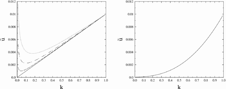
Figure 1: Scaling of the dimensionless coupling constant $\tilde{u}$ for $\beta^{2}=12\pi$ (to the left) and for $\beta^{2}=18\pi$ (to the right), according to Eq. (43), for the LSG model. In the figure to the left, the solid line represents the UV scaling law obtained according to Eq. (26), and the dashed, dashed-dotted and the dotted lines illustrate the mass-corrected UV scaling laws for various values of $J=0.002,\,0.01,\,0.03$, respectively. For the computations, the UV scale has been chosen as $\Lambda=1$.

If $\beta^{2}>\beta^{2}_{c}=16\pi$, the Fourier amplitude $\tilde{u}$ remains an irrelevant coupling constant even in the IR region. This suggests that the LSG model may exhibit two phases, separated by the Coleman fixed point. The coupling $u$, which plays the role of the fugacity of the layered vortex gas has a completely different behaviour in these two phases. The critical value (critical temperature) for the layered system $\beta_{c}^{2}=16\pi$ persists; this critical value holds irrespective of the mass eigenvalue $M_{+}^{2}=2J$, the only criterium being that $M_{+}^{2}$ should be nonvanishing.

By contrast, if we set $J=0$ explicitly, we arrive at the symmetric massless ML2FSG model with the critical value $\beta_{c}^{2}=8\pi$ [see Eq. (41)]. The limit $J\to 0$ is in that sense nonuniform, and the phase structure is also nonuniform, because an entire symmetry gets restored for $J=0$ (periodicity in both directions of the internal space).

For the LSG model, a preliminary phase diagram, as suggested by the mass-corrected flow, is plotted in Fig. 2. To this end, we have to assume that the mass-corrected UV scaling law (43) holds at least qualitatively in the IR region. This conjecture is supported by numerical calculations, based on the nonlinear terms ${\mathcal{F}}_{2}({\tilde{U}}_{k})$ in Eq. (25), as described below in Sec. 4.4. Preliminary numerical results, based on the full WH RG equation (21) which goes beyond the subleading nonlinear term analyzed in Sec. 4.4, also support this conjecture (the latter calculations will be presented in detail elsewhere).

For the LSG, the broken periodicity in one direction of the internal space leads to

• the existence of two phases with different IR fixed points, ${\tilde{u}}\to\infty$ for $\beta^{2}<\beta_{c}^{2}$ and ${\tilde{u}}\to 0$ for $\beta^{2}>\beta_{c}^{2}$, respectively, and

• an intermediate region in the phase diagram where the UV irrelevant vortex fugacity ${\tilde{u}}$ becomes relevant in the IR scaling regime, after passing a cross-over regime.

In Fig. 1 (regions I and III), the overall scaling behaviour of the vortex fugacity is the same as that for the symmetric ML2FSG model, and in particular, no cross-over regime appears in the flow of $\tilde{u}$. The cross-over regime will be of particular interest for further numerical calculations, based on the full WH RG equation (21).

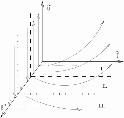
Figure 2: Phase diagram of the LSG model based on the mass-corrected UV scaling law (43). As there is no evolution for $\beta^{2}$ in $d=2$ in the LPA, the RG trajectories lie in planes of constant $\beta^{2}$. The arrows indicate the direction of the flow ($k\to 0$) in which the dimensionless mass eigenvalue $2{\tilde{J}}_{k}=k^{-2}\,2J$ increases. In the $(\tilde{u},~{}\beta^{2})$ plane, the phase diagram of the ML2FSG model ($\tilde{J}=0$) is depicted where the dashed line at $\beta_{c}^{2}=8\pi$ separates the two phases. For the LSG, one finds two phases separated by the plane at $\beta_{c}^{2}=16\pi$ (indicated by the dotted lines). In the phase with $\beta^{2}<16\pi$, two (sub-)regions can be recognized. In region I, the trajectories have the same tendency as for $J=0$: in particular, ${\tilde{u}}$ remains a relevant (increasing) parameter for $k\to 0$. In region II, the UV irrelevant (decreasing) $\tilde{u}$ becomes a relevant (increasing) parameter after a cross-over region. In the phase with $\beta^{2}>16\pi$ (region III), the Fourier amplitude ${\tilde{u}}$ remains irrelevant during the RG flow.

4.3.3 MSG model

It is enlightening to discuss the mass-corrected UV scaling laws for the (one-flavour) MSG model, another particular case with entire breaking of periodicity in the internal space. Formally, the UV scaling laws for the MSG model can be obtained from Eq. (4.3) by setting $M_{1}^{2}=M^{2}$, $M_{2}^{2}=J=0$, which implies that $D=M^{2}/2$ in Eq. (4.3). In this case, flavour symmetry would be broken, but the two flavours actually decouple, and thus we restrict the discussion to a single flavour. We also restrict ourselves to a single Fourier mode in the blocked potential with $(n=1,m=0)$ and the amplitude $\tilde{u}={\tilde{u}}_{10}$. The UV mass-corrected RG evolution reads

$${\tilde{u}}(k) = {\tilde{u}}(\Lambda)\left({k\over\Lambda}\right)^{-2}\left({k^{2}+M^{2}\over\Lambda^{2}+M^{2}}\right)^{\alpha_{2}\beta^{2}/2}.$$ (44)

This reproduces the UV behaviour (26) of the corresponding massless model for scales $M\ll k\sim\Lambda$, where ${\tilde{u}}(k)$ is irrelevant (relevant) for $\beta^{2}>8\pi$ $~{}(<8\pi)$. However, the mass-corrected UV scaling law (44) of the MSG model to the IR limit predicts a cross-over at scales $k^{2}\sim{\mathcal{O}}(M^{2})$ (even) for $\beta^{2}>8\pi$ below which the coupling ${\tilde{u}}(k)$ becomes relevant (see Fig. 3). Thus, irrespective of the choice of $\beta^{2}$, the coupling ${\tilde{u}}(k)$ is suggested to be IR relevant according to the (extrapolation of) the mass-corrected UV scaling law (44) into the IR region.

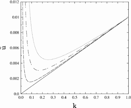
Figure 3: Scaling of the dimensionless coupling constant $\tilde{u}$ of the MSG model for $\beta^{2}=12\pi$. The solid line represents the UV scaling law (26) for the massless SG model. The dashed, dashed-dotted and the dotted lines depict the mass-corrected UV scaling laws (44) for the MSG model, for various values of $M^{2}=0.0036,\,0.0144,\,0.0324$, respectively. In the IR, the mass-corrected RG flow is drastically and qualitatively different from the massless flow, even for small mass parameters, due to the broken internal symmetry.

The mass-corrected UV scaling law in Eq. (44) accounts for the explicit breaking of periodicity in the (one-dimensional) internal space via the nonvanishing mass term and results in the removal of the Coleman fixed point, as compared to the massless case.

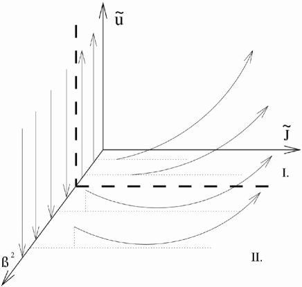
Figure 4: Schematic phase structure of the MSG model based on the analytic solution (44). As in Fig. 2, the results are obtained in the local-potential approximation, where there is no evolution for $\beta^{2}$ and the RG trajectories are always parallel to the $\tilde{M}^{2}=\tilde{J}$ axis. The arrows indicate the direction of the RG flow ($k\to 0$). The WH-RG equation (16) gives a trivial scaling for the coupling ${\tilde{M}^{2}}(k)={\tilde{J}}(k)\propto k^{-2}$ [see Eq. (20)], so that the mass parameters remain relevant couplings during the whole RG flow. The $\tilde{u}$-$\beta^{2}$ plane corresponds to the phase diagram of the massless SG model ($\tilde{M}^{2}=\tilde{J}=0$). The dashed line separates the two phases of the SG (but not the MSG) model. The linearization of the WH equation (22) would predict the same two phases for the MSG model with the same critical value $\beta^{2}=8\pi$. However, the mass-corrected RG treatment modifies this picture and shows only one phase for the MSG model. In region I, the trajectories have the same tendency as in the massless theory; $\tilde{u}\equiv{\tilde{u}}_{01}$ is a relevant (increasing) parameter in the UV and in the IR domain as well. In region II, the UV irrelevant (decreasing) $\tilde{u}$ becomes a relevant (increasing) parameter in the IR limit, after a crossover region, according to Eq. (44).

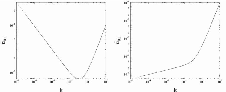
Figure 5: The scaling of the dimensionless coupling constant $\tilde{u}_{01}$ of the LSG model is represented graphically for two different temperature parameters $\beta^{2}=12\pi$ (left) and $\beta^{2}=18\pi$ (right). The interlayer coupling is $J=0.001$ in both cases. The dotted line represents the solution according to Eqs (40) and (43), which is obtained by considering the linear term ${\mathcal{F}}_{1}(\tilde{U}_{k})$ in Eq. (25). The solid line shows the solution of the RG flow including [in addition to ${\mathcal{F}}_{1}(\tilde{U}_{k})$] also the nonlinear term ${\mathcal{F}}_{2}(\tilde{U}_{k})$ in Eq. (25), which leads to the system of equations (45). Both curves almost overlap, which demonstrates that the flow of the fundamental coupling $\tilde{u}_{01}$ is almost independent of the nonlinear corrections mediated by the ${\mathcal{F}}_{2}$ term.

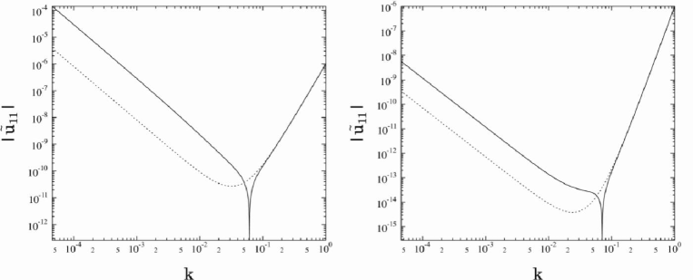
Figure 6: The scaling of the dimensionless coupling constant $|\tilde{u}_{11}|$ (“higher harmonic”) of the LSG model is shown for $\beta^{2}=12\pi$ (left) and $\beta^{2}=18\pi$ (right) and $J=0.001$. The solid and dotted curves are obtained with and without the nonlinear terms, as in Fig. (5), but for a different coupling parameter ($\tilde{u}_{11}$ instead of $\tilde{u}_{01}$), and with an initial condition $\tilde{u}_{11}(\Lambda)=10^{-4}$ at the UV scale $\Lambda=1$. The solution for $\tilde{u}_{11}$, including the nonlinear terms [see Eq. (45)], changes sign near $k\approx 7\times 10^{-2}$ (so that $\ln|\tilde{u}_{11}|\to-\infty$), whereas the flow with linear mass corrections predicts no change of sign (dotted line).

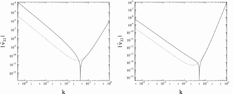
Figure 7: The same as Fig. 6 for the dimensionless coupling constant $|\tilde{v}_{11}|$ (LSG model). In the UV, the two solutions with and without nonlinear terms overlap. In the IR, the two solutions appear to follow similar scaling laws, with approximately equal double-logarithmic derivatives $\partial\ln|{\tilde{v}}_{11}(k)|/\partial\ln k$.

4.4 Extended UV scaling laws for the LSG model

In Secs. 4.3.1, 4.3.2, and 4.3.3, we restricted the discussion to the linear corrections ${{\mathcal{F}}}_{1}(\tilde{U}_{k})$ as listed in Eq. (25). Here we investigate a further modification of the UV scaling laws toward the lower scales, by taking into account the nonlinear term ${{\mathcal{F}}}_{2}(\tilde{U}_{k})$ quadratic in the potential on the right hand side of Eq. (25). For the sake of simplicity, we restrict ourselves to the LSG model. We would like to demonstrate that the nonlinear term ${{\mathcal{F}}}_{2}(\tilde{U}_{k})$ (i) does not change the phase structure obtained on the basis of the mass-corrected UV scaling law (4.3), but (ii) may have a significant effect on the effective potential obtained for $k\to 0$. Thus, one is inclined to suggest that the mass-corrected UV scaling laws enable one to obtain the correct phase structure, although the nonlinearities as implied by the full WH equation (21) play a decisive role in the cross-over region, and for a detailed quantitative analysis of the IR region and the effective potential.

Equating the coefficients of the corresponding Fourier modes on the both sides of Eq. (25), one arrives at the set of equations for the scale-dependent Fourier amplitudes. For the first few Fourier amplitudes $\tilde{u}_{01}=\tilde{u}_{10}$, $\tilde{u}_{11}$ and $\tilde{v}_{11}$, the nonlinear RG equations read

$$(2+k\,\partial_{k})\,\tilde{u}_{01} = \alpha_{2}\,\beta^{2}{\bf F}\,\tilde{u}_{01}$$ (45a)

$$+\alpha_{2}\,\beta^{4}\left[\left({{\bf F}^{2}\over 2}+{\bf G}^{2}\right)\tilde{u}_{01}\,\tilde{u}_{11}-2{\bf F}\,{\bf G}\,\tilde{u}_{01}\,\tilde{v}_{11}\right],$$

$$(2+k\,\partial_{k})\,\tilde{u}_{11} = \alpha_{2}\,\beta^{2}\left[2{\bf F}\,\tilde{u}_{11}-2{\bf G}\,\tilde{v}_{11}\right]+\alpha_{2}\,\beta^{4}\left[{\bf G}^{2}\,\tilde{u}_{01}^{2}\right],$$ (45b)

$$(2+k\,\partial_{k})\,\tilde{v}_{11} = \alpha_{2}\,\beta^{2}\left[2{\bf F}\,\tilde{v}_{11}-2{\bf G}\,\tilde{u}_{11}\right],$$ (45c)

using the notations

$${\bf F}={k^{2}+J\over k^{2}+2J},\hskip 28.45274pt{\bf G}={J\over k^{2}+2J}.$$ (46)

The nonlinear terms generate “higher harmonics.” Specifically, we have the situation that even for vanishing initial values of the couplings of the higher-order Fourier modes at the UV scale $\Lambda$, their nonvanishing values are generated by the fundamental modes $(1,0)$ and $(0,1)$ due to the nonlinear term proportional $\tilde{u}_{01}^{2}$, which can be found on the right hand side of Eqs. (45b). Higher-order Fourier modes with nonvanishing couplings appear in general during the blocking of the LSG model due to the nonlinearities incorporated in the logarithm on the right hand side of Eq. (21). The general ansatz (8) for the blocked potential was motivated by this mixing of the modes and by symmetry considerations.

According to Eq. (43), the coupling $\tilde{u}_{01}(k)$ decreases monotonically with decreasing scale $k$, but its logarithmic slope $\partial\ln\tilde{u}_{01}(k)/\partial\ln k$ is predicted to change from $-2+\alpha_{2}\beta^{2}$ for $J\ll k^{2}<\Lambda^{2}$ to $-2+\alpha_{2}\beta^{2}/2$ for $k^{2}\ll J$. The couplings of the higher harmonics should be irrelevant in the UV: both $|\tilde{u}_{11}(k)|$, and $|\tilde{v}_{11}(k)|$ should be proportional to $k^{-2+2\alpha_{2}\beta^{2}}$. Equation (43) also predicts that $|\tilde{u}_{11}(k)|$, and $|\tilde{v}_{11}(k)|$ should become relevant in the IR region, following essentially the tree-level scaling $\sim k^{-2}$.

As shown in Figs. 5—7, these basic features are not modified by the nonlinear terms. Numerical solutions of Eq. (45) are found for initial conditions which are chosen so that $|\tilde{u}_{01}(\Lambda)|\gg|\tilde{u}_{11}(\Lambda)|$ and $|\tilde{u}_{01}(\Lambda)|\gg|\tilde{v}_{11}(\Lambda)|$ at the UV scale, and $\beta^{2}$ assumes the values of $12\pi$ and $18\pi$ (see Figs. 5—7). The scaling of the fundamental modes $\tilde{u}_{01}(k)$ is only marginally influenced by the nonlinear terms (Fig. 5). The situation is somewhat different for $\tilde{u}_{11}(k)$ and $\tilde{v}_{11}(k)$. If the nonlinear terms are added, then the couplings $\tilde{u}_{11}(k)$ and $\tilde{v}_{11}(k)$ change sign in the cross-over region. The flow diagrams reflect the same phase structure as obtained on the basis of the mass-corrected UV scaling laws. In particular, the fact that the couplings $\tilde{u}_{11}(k)$ and $\tilde{v}_{11}(k)$ follow the tree-level scaling in the IR region ($\propto k^{-2}$) means that the dimensionful couplings (obtained via multiplication by $k^{2}$) tend to nonvanishing finite constants in the limit $k\to 0$. For $\beta^{2}<\beta_{c}^{2}$, the fundamental dimensionful coupling $u_{01}$ behaves similarly, whereas for $\beta^{2}>\beta_{c}^{2}$ it tends to zero. Thus, one expects—in both phases—a nonvanishing periodic piece of the effective potential, as opposed to the massless SG model when the periodic effective potential should be a trivial constant due to the requirement of convexity [10, 29].

5 Summary

The differential renormalization group (RG) in momentum space with a sharp cut-off (Wegner’s and Houghton’s method) has been applied in the local potential approximation (LPA) to a general two-flavour massive sine-Gordon (2FMSG) model, as defined in Sec. 2. The ansatz used for the blocked potential contains a mass term and a contribution which is periodic in the different directions of the internal space [see Eq. (15)]. The bare Lagrangians under study have only one nonvanishing Fourier mode [see Eq. (28)]. Particular attention has been paid to the layered sine-Gordon (LSG) model, as defined in Eq. (11), which is the bosonized version of the multi-flavour Schwinger model. In general, we consider models with two flavours (two interacting scalar quantum fields) with an interaction periodic in the internal space spanned by the field variables.

For the massive SG-type models, the usual perturbative approach to renormalization is not applicable. One should preserve the symmetry of the periodic part keeping the Taylor expansion of the potential intact. “Polynomial” self-interactions proportional to $\phi^{n}$, obtained by the Taylor expansion of the periodic potential, should be summed up and considered as one composite operator [which might be of the form $\cos(\beta\phi)$]. This can only be achieved in the framework of non-perturbative renormalization group methods.

It has been shown that the dimensionful mass matrix remains constant in the LPA, under the RG flow. The explicit breaking of the periodicity by mass terms modifies the properties of the scaling laws and the periodic blocked potential significantly. UV scaling laws for the massless SG models exhibit a Coleman fixed point. For massive models, the determination of the UV scaling laws has to include mass corrections (see Sec. 4). When periodicity is partially broken, with one nonvanishing mass eigenvalue, the Coleman fixed point is found to be shifted. With an entirely broken periodicity, we find a complete disappearance of the Coleman fixed point.

For the particular case of the LSG model, periodicity is only partially broken, and the existence of two phases is suggested by the RG flow. The fundamental mode ${\tilde{u}}_{01}$ of the periodic potential is irrelevant and relevant in the IR scaling region, depending on whether $\beta^{2}>16\,\pi$ or $\beta^{2}<16\,\pi$, respectively. The RG flow of the UV irrelevant amplitude of the fundamental mode may pass a cross-over region ($8\,\pi<\beta^{2}<16\,\pi$), before becoming relevant in the IR regime. The mass-corrected RG flow is beyond the “dilute gas approximation” which would correspond to the flow given by Eq. (22).

In view of our analysis of the S2FMSG (Sec. 4.3.1), of the LSG (Secs. 4.3.2 and 4.4) and the MSG model (Sec. 4.3.3), we may suggest that the Coleman fixed point disappears, when periodicity is explicitly broken by mass terms in both independent directions of the internal space. Thus, one expects the existence of a single phase for the MSG model (see Fig. 4). Of course, a final and definite conclusion would require a full numerical solution of the flow equation (21) for these models. However, we are in the position to remark that preliminary numerical results appear to support the results based on the mass-corrected UV RG flow, as reported in the current article. The interesting cross-over region, as shown in Figs. 2 and 4, suggests that the numerical determination of the effective potential can provide operators, which are relevant for IR physics although they are irrelevant at the UV scale.

The subleading nonlinear terms in RG flow have been analyzed in Sec. 4.4, which is a step toward the full solution of the WH equation (21). The nonlinear terms are quadratic in the periodic blocked potential. Due to the nonlinearity of the flow, higher order Fourier modes, normally suppressed at the UV cut-off, appear in the periodic blocked potential. For the LSG model, it has been demonstrated that the quadratic nonlinear terms play a negligible role for the RG evolution of the fundamental coupling ${\tilde{u}}_{01}$, provided the higher harmonics are suppressed at the UV scale (as it should be in view of the given structure of the bare Lagrangians). However, the nonlinear terms play an important role in the behaviour of the UV irrelevant couplings of the higher harmonics in the cross-over region.

Another rather surprising aspect concerns the structure of the effective potential for theories with a nonvanishing mass matrix as opposed to their massless counterparts: namely, for the “massive” case, one expects a nonvanishing periodic of the effective potential, as opposed to the massless SG model, where the simultaneous requirements of periodicity and convexity result in a field-independent effective potential.

Appendix A Bosonization of the Multi-Flavour Schwinger Model

In this section, we dwell on the fact that the MSG model (12) and the LSG model (11) are the theories obtained by bosonization from the massive Schwinger model (1+1 dimensional QED) obeying $U(1)$ and $SU(2)$ global flavour symmetries, respectively. The multi-flavour Schwinger model has not been studied as extensively as the massive Schwinger model, the case with $U(1)$ flavour symmetry. The latter proved to be interesting since it shows confinement properties. However, the relative ignorance toward the multi-flavour Schwinger model is perhaps not fully justified as it shows more resemblance to the 4-dimensional QCD, because the model features a chiral symmetry breakdown [3].

Two–dimensional QED with an $SU(2)$ internal symmetry can be characterized by the Lagrangian

$${\mathcal{L}}=\sum_{i=1,2}\bar{\psi}_{i}(\mbox{$\partial\!\!\!/$}-m-e\mbox{$A\!\!\!/$})\psi_{i}-\frac{1}{4}F_{\mu\nu}F^{\mu\nu}\,.$$ (47)

Here $A_{\mu}$ is the vector potential of the photon field. The $\psi_{i}$ ($i=1,2$) denote an $SU(2)$ flavour-doublet of fermions. Furthermore, the field-strength tensor is given by $F_{\mu\nu}=\partial_{\mu}A_{\nu}-\partial_{\nu}A_{\mu}$, and $m$ and $e$ are the bare rest mass of the electron and the bare coupling constant, respectively. The model (47) was shown to be capable [4] of describing materials with a zero net charge, but with a non-zero flavour charge, interpreted as ‘baryon number’ density, a kind of matter in neutron stars. Bosonization of the model (47) proceeds according to the following rules [26, 27, 28],

$$:\bar{\psi}_{i}\psi_{i}: \to -cmM\cos(2\sqrt{\pi}\phi_{i}),$$ (48a)

$$:\bar{\psi}_{i}\gamma_{5}\psi_{i}: \to -cmM\sin(2\sqrt{\pi}\phi_{i}),$$ (48b)

$$:\bar{\psi}_{i}\gamma_{\mu}\psi_{i}: \to \frac{1}{\sqrt{\pi}}\varepsilon_{\mu\nu}\partial^{\nu}\phi_{i},$$ (48c)

$$:\bar{\psi}_{i}i\mbox{$\partial\!\!\!/$}\psi_{i}: \to \frac{1}{2}N_{m}(\partial\phi_{i})^{2},$$ (48d)

where $i=1,2$, and there is no sum on $i$. Here, $N_{m}$ denotes normal ordering with respect to the fermion mass $m$, and $c=\exp{(\gamma)}/2\pi$ with the Euler constant $\gamma$. In the case of an equal mass and opposite charges of the two fermions, the bosonized form of the theory becomes

$${\mathcal{H}} = N_{m}\biggl{[}\frac{1}{2}\Pi_{1}^{2}+\frac{1}{2}\Pi_{2}^{2}+\frac{1}{2}(\partial_{1}\phi_{1})^{2}+\frac{1}{2}(\partial_{1}\phi_{2})^{2}$$ (49)

$$-cm^{2}\cos(2\sqrt{\pi}\phi_{1})-cm^{2}\cos(2\sqrt{\pi}\phi_{2})-\frac{e^{2}}{2\pi}(\phi_{1}-\phi_{2})^{2}\biggr{]}\,.$$

The theory defined by the Hamiltonian (49) is identical to the LSG model (11) under an appropriate identification of the coupling constants of the two models ($\beta^{2}=4\pi$).

Appendix B Some notes on the Wegner-Houghton equation

As has already been mentioned in Sec. 3, the WH-RG equation has to be projected into a particular functional subspace, in order to reduce the search for a functional (the blocked action) to the calculation of an appropriate function. Here, we assume that the blocked action contains only local interactions. We use the approach outlined in [13, 11], expand it in powers of the gradients of the fields $\phi_{1}$ and $\phi_{2}$, and keep only the leading-order terms; thus we arrive at an ansatz for the blocked action. Indeed, for the $d=2$ LSG-type models with two scalar fields $\phi_{1}$ and $\phi_{2}$, the blocked action reads

$$S_{k}=\,\int{\mathrm{d}}^{2}x\left[{1\over 2}\,(\partial\phi_{1})^{2}+{1\over 2}(\partial\phi_{2})^{2}\,+\,V_{k}(\phi_{1},\phi_{2})\right]\,.$$ (50)

The evolution of the blocked potential $V_{k}$ in the direction of decreasing $k$ is supposed to be satisfying the following generalized WH-RG equation for two interacting fields in $d=2$,

$$k\,\partial_{k}V_{k}=-{k^{2}\over 4\pi}\ln\left({[k^{2}+V^{11}_{k}][k^{2}+V^{22}_{k}]-[V^{12}_{k}]^{2}\over k^{4}}\right)\,,$$ (51)

where

$$V^{ij}_{k}\equiv\partial_{\phi_{i}}\partial_{\phi_{j}}V_{k}\,.$$ (52)

We recall that $V_{k}$ is a function of functions $\phi_{i}$, so that the differentiations with respect to the $\phi_{i}$ and to the $k$ need to be carefully distinguished. The equation (51) is nonperturbative as it does not imply an expansion of $V_{k}$ in powers of its arguments $\phi_{1}$ and $\phi_{2}$. The derivation of the (generalized) WH equation (51) for two-component models has been inspired by techniques outlined for ${\mathcal{O}}(N)$-symmetric models [12].

One actually has a certain freedom in constructing the WH equation, which becomes apparent when adding to the Euclidean action in (50) a field-independent term. This freedom generates a class of WH equations characterized by the structure

$$k\,\partial_{k}V_{k}=-{k^{2}\over 4\pi}\ln\left({[k^{2}+V^{11}_{k}][k^{2}+V^{22}_{k}]-[V^{12}_{k}]^{2}\over f(k)}\right)\,,$$ (53)

with the requirement that ${\rm dim}f(k)={\rm dim}\,k^{4}$, and this freedom gives us the possibility to discard the term $\ln(1+{\tilde{\mu}}^{2})$ on the right hand side of (24). The WH-RG equation (51), rewritten in terms of dimensionless quantities, yields Eq. (16).

The dimensionless WH-RG equation (16) is applicable for the LSG type models defined in Sec. 2, and one can solve it for a particular field-theoretical model by projecting $\tilde{V}_{k}$ onto a particular space of functions, with appropriate UV boundary conditions for the RG evolutions. Of course, the functional ansatz for the blocked potential should be rich enough in order to ensure that the RG flow does not leave the chosen subspace of blocked potentials, and it should preserve all symmetries of the original model at the UV cutoff scale $k=\Lambda$. For example, the blocked potential for the LSG model should be invariant under the exchange of the field variables, $\phi_{1}\leftrightarrow\phi_{2}$ because the layers are physically equivalent, and it should also preserve the symmetries $\phi_{i}\to-\phi_{i}$ and $\phi_{i}\to\phi_{i}+2\pi/\beta$ which are present in the bare Lagrangian. In the cases of interest for the current study, all these requirements are fulfilled by the ansatz (8) for the dimensionless blocked potential.

References

- [1] J. C. Le Guillou, J. Zinn-Justin, Phys. Rev. B21 (1980) 3976.
- [2] R. Guida, J. Zinn-Justin, Nucl. Phys. B489 (1996) 626.
- [3] J. E. Hetrick, Y. Hosotani, S. Iso, Phys. Lett. B350 (1995) 92.
- [4] W. Fischler, J. Kogut, L. Susskind, Phys. Rev. D19 (1979) 1188.
- [5] N. D. Mermin, H. Wagner, Phys. Rev. Lett. 17 (1966) 1133.
- [6] J. M. Kosterlitz, D. J. Thouless, J. Phys. C6 (1973) 118.
- [7] J. M. Kosterlitz, J. Phys. C7 (1974) 1046.
- [8] J. V. Jose, L. P. Kadanoff, S. Kirkpatrick, D. R. Nelson, Phys. Rev. B16 (1977) 1217.
- [9] G. von Gersdorff, C. Wetterich, Nonperturbative renormalization flow and essential scaling for the Kosterlitz-Thouless transitions, e-print hep-th/0008114.
- [10] I. Nándori, J. Polonyi, K. Sailer, Phys. Rev. D63 (2001) 045022.; Phil. Mag. B81 (2001) 1615.
- [11] J. Zinn-Justin, Groupe de renormalisation fonctionnel, 2004 (unpublished); Groupe de renormalisation fonctionnel et équations de champs, 2004 (unpublished).
- [12] G. Eyal, M. Moshe, S. Nishigaki, J. Zinn-Justin, Nucl. Phys. B470 (1996) 369.
- [13] J. Polonyi, Central Eur. J. Phys. 1 (2004) 1; Lectures on the functional renormalization group method, e-print hep-th/0110026.
- [14] K. G. Wilson, Phys. Rev. D3 (1971) 1818.
- [15] S. Nagy, J. Polonyi, K. Sailer, Phys. Rev. D70 (2004) 105023.
- [16] S. W. Pierson, Phys. Rev. Lett. 74 (1995) 2359; Phys. Rev. B55 (1997) 14536.
- [17] S. W. Pierson, O. T. Valls, Phys. Rev. B49 (1994) 662.
- [18] S. W. Pierson, O. T. Valls, Phys. Rev. B45 (1992) 13076.
- [19] S. W. Pierson, O. T. Valls, H. Bahlouli, Phys. Rev. B45 (1992) 13035.
- [20] I. Nándori and K. Sailer, to be published in Phil. Mag., see also e-print hep-th/0508033.
- [21] I. Nándori, K. Vad, S. Mészáros, J. Hakl, B. Sas, Czech. J. Phys. 54 (2004) D481.
- [22] K. Vad, S. Mészáros, I. Nándori, B. Sas, to be published in Phil. Mag., see also e-print cond-mat/0508146; K. Vad, S. Mészáros, B. Sas, to be published in Physica C, see also e-print cond-mat/0508184.
- [23] D. Delpenich, J. Schechter, Int. J. Mod. Phys. A12 (1997) 5305.
- [24] A. Smilga, J. J. M. Verbaarschot, Phys. Rev. D54 (1996) 1087.
- [25] F. J. Wegner, A. Houghton, Phys. Rev. A8 (1973) 401.
- [26] S. Coleman, Commun. Math. Phys. 31 (1973) 259.
- [27] S. Coleman, Phys. Rev. D11 (1975) 2088.
- [28] S. Coleman, Ann. Phys. 101 (1976) 239.
- [29] I. Nándori, K. Sailer, U. D. Jentschura, G. Soff, Phys. Rev. D69 (2004) 025004; J. Phys. G28 (2002) 607.