Quasinormal modes for nonextreme D$p$-branes
and
thermalizations of super-Yang-Mills theories

Abstract

The nonextreme D$p$-brane solutions in type II supergravity (in the near-horizon limit) are expected to be dual to $(p+1)$-dimensional noncompact supersymmetric Yang-Mills theories at finite temperature. We study the translationally invariant perturbations along the branes in those backgrounds and calculate quasinormal frequencies numerically. These frequencies should determine the thermalization time scales in the dual Yang-Mills theories.

I Introduction

As with any dualities, gauge/gravity dualities or AdS/CFT dualities (anti-deSitter/conformal field theory dualities) are interesting in two respects. are interesting in two respects. On one side, supergravities give information of dual Yang-Mills theories in strong coupling regimes such as confinement.

On another side, Yang-Mills theories give information of supergravities. Finite temperature gauge/gravity duals are particularly interesting in this respect. The original finite temperature gauge/gravity duality is the duality between ${\cal N}=4$ finite temperature super-Yang-Mills theory (SYM) and type IIB string theory in the Schwarzschild-${\rm AdS}_{5}$ (${\rm SAdS}_{5}$) $\times S^{5}$ background Witten:1998zw . Thus, finite temperature gauge/gravity dualities should address long-standing puzzles in gravity, such as the singularity problem Kraus:2002iv ; Hong Liu:2005  (and references therein), the information paradox Maldacena:2001kr ; Hawking:2005kf , and the Gregory-Laflamme instability GL ; Aharony:2004ig .

Unfortunately, finite temperature gauge/gravity dualities have been less studied compared with the zero-temperature AdS/CFT. First, many evidences of finite temperature gauge/gravity dualities remain qualitative. Most well-known evidences are

1. The existence of the confinement-deconfinement transition (the Hawking-Page transition in gravity side Hawking:1982dh )

2. The large-$N$ dependence of the partition function in each phase

but quantitative understandings are still far. (The lack of supersymmetry for finite temperature is obviously the main obstacle.) Second, backgrounds other than ${\rm SAdS}_{5}$ have been less studied compared with the zero-temperature cases.

This paper provides one step toward these directions. The original AdS/CFT duality is motivated by the near-horizon limit of the extreme D3-brane. But the similar dualities are expected for the other D$p$-branes (if $p<5$) Itzhaki:1998dd . They are expected to dual to $(p+1)$-dimensional SYM. Some qualitative features have been known for these dualities, but there are less quantitative studies. (Various Wilson loops have been computed, e.g., see Ref. Brandhuber:1998er and references therein. At the zero temperature, the correlation functions are computed in Ref. Sekino:1999av .)

Our aim is to compute the quasinormal (QN) frequencies in these backgrounds. It is an important concept in black hole physics and has been widely discussed in the literature. Moreover, the QN frequencies of an AdS black hole have an interpretation in the dual gauge theory. Such a black hole corresponds to a thermal state in the gauge theory. The QN frequencies measure how perturbations of black holes decay. In the dual theory, this corresponds to the process where a perturbation of the thermal state decays and the system returns to the thermal equilibrium. Thus, QN frequencies give the prediction of the thermalization time scale for the strongly-coupled gauge theory HoHu ; MossNorman ; BK ; CKL ; Konoplya ; ref:MusiriSiopsis . It has been also argued that these modes govern the behavior of gauge theory plasmas. (See, e.g., Refs. Benincasa:2005iv ; Policastro:2002se ; ref:Starinets ; ref:NunezStarinets ; ref:KovtunStarinets and references therein.)

The plan of the present paper is as follows. First, in the next section, we review gauge/gravity dualities for D$p$-branes. In section III, we present the perturbed equations which are translationally invariant along the brane, and briefly review a simple numerical method HoHu to obtain QN frequencies. In section IV, we discuss the numerical results. We conclude in section V with a summary of our results. In the Appendix, we briefly review QN modes for readers not having sufficient background in them.

II Gauge/gravity dualities for D$p$-branes

II.1 Bulk geometry

In this Section, we quickly review gauge/gravity dualities for D$p$-branes. The relevant part of type II supergravity action is given by

$$S=\frac{1}{(2\pi)^{7}l_{s}^{8}}\int d^{10}x\sqrt{-G}\left[~{}e^{-2\phi}~{}\Bigl{(}R+4(\nabla\phi)^{2}\Bigr{)}-\frac{1}{2(p+2)!}F_{p+2}^{2}~{}\right].$$ (1)

The nonextreme D$p$-branes are written as

$$ds^{2} = Z_{p}^{-1/2}(-hdt^{2}+d\vec{x}_{p}^{2})+Z_{p}^{1/2}(h^{-1}dr^{2}+r^{2}d\Omega_{8-p}^{2}),$$

$$g_{s}^{2}e^{-2\phi} = Z_{p}^{\frac{p-3}{2}},$$ (2)

where $g_{s}=e^{\phi_{\infty}}$ and the harmonic functions are given by

$$Z_{p}(r) = 1+\left(\frac{r_{p}}{r}\right)^{7-p},\qquad r_{p}^{7-p}\sim g_{s}Nl_{s}^{7-p},$$ (3)

$$h(r) = 1-\left(\frac{r_{0}}{r}\right)^{7-p}.$$ (4)

Let us take the “decoupling” limit or the “near-horizon” limit. In order to take the limit, we assume $r\sim r_{0}\ll r_{p}$. Then, $Z_{p}=1+(r_{p}/r)^{7-p}\rightarrow(r_{p}/r)^{7-p}$.

Introducing a new coordinate $\tilde{r}$,

$$\frac{r}{r_{p}}=\left(\frac{2}{5-p}\right)^{\frac{2}{5-p}}\left(\frac{\tilde{r}}{r_{p}}\right)^{\frac{2}{5-p}},$$ (5)

the metric becomes

$$ds^{2} \simeq \left(\frac{2}{5-p}\right)^{2}\left(\frac{r}{l}\right)^{\frac{p-3}{2}}\left[-\tilde{H}(\tilde{r})dt^{2}+\left(\frac{\tilde{r}}{l}\right)^{2}d\vec{x}_{p}^{2}+\frac{d\tilde{r}^{2}}{\tilde{H}(\tilde{r})}+\left(\frac{5-p}{2}l\right)^{2}d\Omega^{2}_{8-p}\right],$$ (6)

where $l=r_{p}$. $\tilde{H}$ and $\phi$ are rewritten as

$$\tilde{H}(\tilde{r}) = \left(\frac{\tilde{r}}{l}\right)^{2}-\left(\frac{\tilde{r}_{0}}{l}\right)^{\frac{2(7-p)}{5-p}}\left(\frac{\tilde{r}}{l}\right)^{-\frac{4}{5-p}},$$

$$g_{s}^{2}e^{-2\phi} = \left(\frac{5-p}{2}\frac{l}{\tilde{r}}\right)^{\frac{(7-p)(p-3)}{5-p}}.$$ (7)

It is clear that the metric is conformal to ${\rm AdS}_{p+2}\times S^{8-p}$ asymptotically if $p<5$. Solutions with $p\geq 5$ do not have a positive specific heat, so we consider $p<5$. We shall use such a “AdS-frame” to calculate QN frequencies.

As is well-known, the above metric is not the ${\rm SAdS}$ solution even if $p=3$. The ${\rm SAdS}_{5}$ solution is given by

$$ds^{2}=-\left(\frac{\tilde{r}^{2}}{l^{2}}+1-\frac{\tilde{r}_{0}^{4}}{l^{2}\tilde{r}^{2}}\right)dt^{2}+\left(\frac{\tilde{r}^{2}}{l^{2}}+1-\frac{\tilde{r}_{0}^{4}}{l^{2}\tilde{r}^{2}}\right)^{-1}d\tilde{r}^{2}+\tilde{r}^{2}d\Omega_{3}^{2}.$$ (8)

${\rm SAdS}_{5}$ has the horizon with the topology of $S^{p}$, whereas the metric (6) has the horizon with the topology $R^{p}$. We call such solutions “planar black holes.”  The $p=3$ planar black hole corresponds to the large black hole limit of ${\rm SAdS}_{5}$. In order to reach the planar black hole from ${\rm SAdS}_{5}$, rescale the coordinates

$$t~{}\rightarrow~{}t/\alpha,\qquad\qquad\tilde{r}~{}\rightarrow~{}\alpha\,\tilde{r},\qquad\qquad{\rm and}\qquad\qquad\tilde{r}_{0}~{}\rightarrow~{}\alpha\,\tilde{r}_{0}.$$ (9)

Then, the $S^{3}$ radius is proportional to $\alpha$, so $\alpha^{2}d\Omega_{3}^{2}\sim\sum d\vec{x}_{p}{}^{2}$ for large $\alpha$. This limit, the planar ${\rm SAdS}_{5}$ black hole, is invariant under the above scaling.

We consider such planar black holes from the following reasons. First, AdS black hole solutions with $S^{p}$ topology are not known when the dilaton is nontrivial. Second, in the SYM description, SAdS corresponds to a compact SYM on $S^{p}$, and a planar black hole corresponds to a noncompact SYM on $R^{p}$. The motivation to consider a compact SYM in Ref. Witten:1998zw is to break the scale invariance (9). Without breaking the scale invariance, one cannot see the confinement/deconfinement transition in gauge theory. Here, there is no scale invariance due to the dilaton. So, it is not clear whether one should consider a compact SYM.

II.2 Validity of supergravity descriptions

To discuss the validity of supergravity description (6), it is convenient to introduce SYM variables. The SYM coupling in terms of string variables are (See, e.g., Ref. Polchinski:1998rr )

$$g_{YM}^{2}=(2\pi)^{p-2}\,g_{s}\,l_{s}^{p-3},$$ (10)

where $g_{YM}$ is the $(p+1)$-dimensional SYM coupling constant. The effective (dimensionless) coupling of SYM theories is

$$g_{eff}^{2}=g_{YM}^{2}\,N\,\left(\frac{r}{l_{s}^{2}}\right)^{p-3}.$$ (11)

The SYM perturbation theory can be trusted in the region

$$g_{eff}\ll 1.$$ (12)

On the other hand, one can trust supergravity solutions if both the curvature (in string metric) and the dilaton are small. Since

$$e^{\phi}\sim g_{eff}^{(7-p)/2}/N~{}, l_{s}^{2}\,R\sim 1/g_{eff}~{},$$ (13)

these conditions imply

$$1\ll g_{eff}^{2}\ll N^{4/(7-p)}.$$ (14)

Clearly, the perturbative SYM and supergravity descriptions do not overlap. For $p<3$, this gives the following range of $r$ (not the AdS-like coordinate $\tilde{r}$):

$$(g_{YM}^{2}N)^{1/(3-p)}N^{-4/(3-p)(7-p)}\ll r/l_{s}^{2}\ll(g_{YM}^{2}N)^{1/(3-p)}~{}.$$ (15)

(For $p>3$, replace the $\ll$ signs by $\gg$ signs.) The left-hand side and the right-hand side of these inequalities come from the dilaton and the curvature, respectively. They have a diverging dilaton at $r=0$ and a curvature singularity at $r=\infty$. One necessary condition to satisfy the above condition is $N\gg 1$.

When the radial coordinate $r$ is outside the region, different theories (such as M-theory) take over the type II descriptions. The radial coordinate has the gauge theory interpretation as the energy scale. The phase diagrams are discussed in Ref. Itzhaki:1998dd . For type IIA-branes, the M-brane description take over at small radius. As argued later, the M-brane description often reduces to a SAdS black hole, and there have been extensive works on the subject; this limit is relatively well-known. The other limit is the perturbative SYM description at large radius; again this limit is rather well-known. Therefore, we focus on the intermediate energy scale where type II supergravity is a valid description.

In order to calculate QN frequencies, one places boundary conditions both at the horizon and at infinity. We henceforth consider the case where the horizon radius lies inside the region (15). In the large-$N$ limit ($N\rightarrow\infty$ and $g_{YM}\rightarrow 0$ with a fixed large $g_{YM}^{2}N$), one can enlarge this region as large as one wishes. Type II description is not a good description at infinity as well. One might put a boundary condition at a large radius but within the region of the validity. We here assume that such a boundary condition at large radius does not affect the results significantly. We return to the issue of the validity and discuss how different boundary conditions may affect our results in Sect. IV.3.

III Numerical approaches for QN frequencies

III.1 Basic equations

After the conformal transformation of the metric (II.1),

$$d\tilde{s}^{2}=\left(\frac{5-p}{2}\right)^{2}(g_{s}e^{-\phi})^{\frac{1}{7-p}}ds^{2}=\tilde{G}_{MN}\,dx^{M}\,dx^{N},$$ (16)

the action (1) is transformed as

$$S=\int d^{10}x\sqrt{-\tilde{G}}\left[~{}e^{2a\phi}\Big{(}\tilde{R}+4b(\tilde{\nabla}\phi)^{2}\Big{)}-\frac{\gamma^{2(p+1)}e^{-2a\phi}}{2(p+2)!}\tilde{F}_{p+2}^{2}~{}\right],$$ (17)

up to a constant, where

$$a=\frac{p-3}{7-p},\qquad b=\frac{(p-1)(p-4)}{(7-p)^{2}},\qquad\gamma=\frac{5-p}{2}~{}g_{s}^{\frac{1}{7-p}}.$$ (18)

Since we are not interested in the perturbation on $S^{8-p}$ sphere, we assume an ansatz for the metric:

$$d\tilde{s}^{2}=\underline{g}_{\mu\nu}(x^{\rho})dx^{\mu}dx^{\nu}+\left(\frac{5-p}{2}\,l\right)^{2}d\Omega^{2}_{8-p},$$ (19)

where $\Lambda=-\frac{1}{l^{2}}\frac{(9-p)(7-p)}{(5-p)^{2}}$ and greek indices run from $0$ to $p+1$. After the compactification, one gets a $(p+2)$-dimensional action Townsend

$$S = \int d^{p+2}x~{}\sqrt{-\underline{g}}~{}e^{2a\phi}~{}\Big{(}\underline{R}-2\Lambda+4b\,(\underline{\nabla}\phi)^{2}\Big{)}~{},$$ (20)

up to a constant. The $p=0$ case reduces to two-dimensional gravity coupled to a scalar, so the system locally has no dynamical degrees of freedom. Hereafter, we focus on $1\leq p\leq 4$.

For simplicity, we shall only consider the perturbations which are translationally invariant along the brane. Then, one can set the metric as

$$d\underline{s}_{(p+2)}^{2}=\underline{g}_{\mu\nu}\,dx^{\mu}dx^{\nu}={}^{(2)}\!g_{ab}(x^{c})\,dx^{a}dx^{b}+e^{2\zeta(x^{a})}\,d\vec{x}_{p}{}^{2}~{},$$ (21)

where $x^{a}=(t,\tilde{r})$. And the action (20) becomes

$$S=\int d^{2}x~{}\sqrt{-{}^{(2)}\!g}~{}e^{\psi_{2}}\left[~{}{}^{(2)}\!R-2\,\Lambda-\frac{p\,(p-3)^{2}}{9-p}\,\left({}^{(2)}\!\nabla\psi_{1}\right)^{2}+\frac{4}{9-p}\left({}^{(2)}\!\nabla\psi_{2}\right)^{2}~{}\right]~{},$$ (22)

where

$$\psi_{1}=\frac{5-p}{(7-p)(p-3)}~{}2\,\phi-\zeta~{}, \psi_{2}=2a\,\phi+p\,\zeta~{},$$ (23)

The system is two-dimensional gravity coupled to two scalars, $\psi_{1}$ and $\psi_{2}$, and there is only one dynamical degrees of freedom. We need to find the dynamical degrees of freedom and obtain its perturbative equation around the background solutions given by Eqs.(6) and (7). Fortunately, since the background solution for $\psi_{1}$ is constant, it is easy to show that its perturbation $\delta\psi_{1}$ is gauge invarint at the perturbative level ref:KodamaSasaki , and the equation of motion is given by

$$0=\partial_{a}\left[~{}\sqrt{-{}^{(2)}\!\bm{g}}~{}{}^{(2)}\!\bm{g}^{ab}~{}e^{\bm{\psi}_{2}}~{}\partial_{b}\,\delta\psi_{1}~{}\right]~{},$$ (24)

where the bold face letters are background quantities.

One can show that this equation is invariant under the scaling (9) with $l$ fixed. By the same argument as in Ref. HoHu , this scale invariance means that QN frequencies are proportional to $\tilde{r}_{0}$, or the black hole temperature $T\propto\tilde{r}_{0}/l^{2}$. Hence, it is convenient to introduce dimensionless coordinates $\tau=\tilde{r}_{0}\,t/l^{2}$ and $\eta=\tilde{r}/\tilde{r}_{0}$, and

$$Z=e^{\bm{\psi}_{2}/2}~{}\delta\psi_{1}~{}.$$ (25)

Then, Eq.(24) is rewritten by

$$-\partial_{\tau}^{2}Z=\left(-\partial_{\eta_{*}}^{2}+V\,\right)\,Z=\big{[}~{}-H\partial_{\eta}(H\partial_{\eta})+V~{}\big{]}\,Z~{},$$ (26)

where

$$H=\eta^{2}(1-\eta^{-q})~{}, V=\nu\,H~{}\big{(}\nu+1+\nu\,\eta^{-q}\big{)}~{},$$ (27)

$$\nu=\frac{9-p}{2(5-p)}~{}, q=\frac{2(7-p)}{5-p}~{},$$ (28)

and the tortoise coordinate $\eta_{*}$ is defined by

$$\eta_{*}=\int d\eta/H~{}.$$ (29)

The potential $V$ is monotonically increasing function of $\eta$ and $V\,|_{\eta=1}=0$, so the potential $V$ is positive-definite outside the horizon ($\eta>1$).

III.2 A numerical method to obtain QN frequencies

Following Horowitz and Hubney’s method HoHu , let us calculate the QN frequencies for D$1$, D$2$, and D$4$-branes. For the later convenience, we shall define $\psi$ as

$$Z=e^{-i\hat{\omega}\tau}(1-\eta^{-q})^{-i\hat{\omega}/q}~{}\psi(\eta)~{},$$ (30)

and introduce a new coordinate $x=\eta^{-2\sigma/(5-p)}$, where $\sigma=1$ for $p=$ even and $\sigma=2$ for $p=$ odd. When $p<5$, the horizon and the infinity correspond to $x=1$ and $x=0$, respectively. Then, one gets a Fuchs-type differential equation:

$$s(x)\frac{d^{2}}{dx^{2}}\,\psi(x)+\frac{t(x)}{x-1}\,\frac{d}{dx}\,\psi(x)+\frac{u(x)}{(x-1)^{2}}\,\psi(x)=0~{},$$ (31)

where

$$s(x)=\left(x\,\frac{x^{(7-p)/\sigma}-1}{x-1}\right)^{2}~{},$$ (32)

$$t(x)=\frac{x}{2\sigma}\,\frac{x^{(7-p)/\sigma}-1}{x-1}~{}\Big{[}~{}5-2\sigma-p+\big{\{}9+2\sigma-p-2i(5-p)\,\hat{\omega}\big{\}}\,x^{(7-p)/\sigma}~{}\Big{]}~{},$$ (33)

$$u(x)=-\left(\frac{5-p}{2\sigma}\right)^{2}\,\Big{[}~{}({\hat{\omega}}+i\,\nu)^{2}\,x^{2(7-p)/\sigma}-(1+2i\,\nu\,\hat{\omega})\,x^{(7-p)/\sigma}-\hat{\omega}^{2}\,x^{(5-p)/\sigma}+\nu(\nu+1)\Big{]}~{}.$$ (34)

We solve these equations by expanding $\psi$ around the horizon ($x=1$). For the power expansion of $\psi$ about $x=1$ to be applicable up to the asymptotic infinity ($x=0$), the radius of convergence must reach $x=0$. Let us examine the singularity structure of Eq.(31) on the complex $x$-plane. Equation (31) has regular singular points when $x=0$ and $x^{(7-p)/\sigma}=1$, namely $x=e^{2\pi i\,\frac{m}{7-p}}\,(m=1,2,\cdots,7-p)$ for $p=$ even and $x=e^{2\pi i\,\frac{2m}{7-p}}\,(m=1,2,\cdots,\frac{7-p}{2})$ for $p=$ odd. So, the nearest singular point of $x=1$ is $x=0$ and the power expansion of $\psi$ about $x=1$ is applicable up to the asymptotic infinity ($x=0$).

The QN modes are the solutions of Eq.(31) with the following boundary conditions:

1. The scalar wave is purely ingoing near the horizon, $Z\sim e^{-i\hat{\omega}(\tau+\eta_{*})}$.

2. The scalar wave decays at infinity, $Z\sim e^{-i\hat{\omega}\tau}\eta^{-(\nu+1)}$.  (Another mode diverges.)

The purely ingoing mode is expressed near the horizon as

$$Z\sim e^{-i\hat{\omega}\tau}e^{-i\hat{\omega}\eta_{*}}=e^{-i\hat{\omega}\tau}e^{-i\hat{\omega}\int d\eta/H}\sim e^{-i\hat{\omega}\tau}(\eta-1)^{-i\hat{\omega}/q}\sim e^{-i\hat{\omega}\tau}(1-\eta^{-q})^{-i\hat{\omega}/q},$$ (35)

which is just the same prefactor in front of $\psi$ in Eq. (30). So, the solution satisfying the condition (i) has the form

$$\psi(x)=\sum^{\infty}_{n=0}a_{n}(x-1)^{n},$$ (36)

where $a_{0}$ is a non-zero constant. Then, the coefficients $a_{n}$ are obtained by the following recursion relation:

$$a_{n}=-\frac{1}{n(n-1)\,s_{0}+n\,t_{0}}~{}\sum^{n-1}_{k=0}~{}[~{}k(k-1)\,s_{n-k}+k\,t_{n-k}+u_{n-k}~{}]\,a_{k}~{},$$ (37)

where $s_{n}$, $t_{n}$, and $u_{n}$ are the $n$-th order coefficients of the expansions around $x=1$, e.g., $s(x)=\sum_{n=1}^{\infty}s_{n}\,(x-1)^{n}$. Since the equations are linear, the coefficient $a_{0}$ is a free parameter (we set $a_{0}=1$).

In order to find the QN frequencies, we need to find the solution satisfying the latter boundary condition (ii):

$$\psi(0)=\sum^{\infty}_{n=0}a_{n}(-1)^{n}=0~{},$$ (38)

which gives a polynomial equation of $\hat{\omega}$.

Before we solve the above equation of $\hat{\omega}$ for $p=1,2$, and $4$ numerically, we comment on some general properties of QN frequencies:

• QN frequencies are symmetrically distributed with respect to the imaginary axis of the complex $\hat{\omega}$-plane, i.e., there is a symmetry $\hat{\omega}~{}\leftrightarrow\,-\hat{\omega}^{*}$.

• The imaginary part of the QN frequency is negative so that the system in our interests is stable.

The former statement is proved as follows: Consider any QNM, $Z_{\hat{\omega}}$ with a QN frequency $\hat{\omega}$. Then, $\big{(}Z_{\hat{\omega}}\big{)}^{*}$ is also a solution of Eq.(26) with the frequency $\hat{\omega}\rightarrow-\hat{\omega}^{*}$. Furthermore, its asymptotic form is $\big{(}Z_{\hat{\omega}}\big{)}^{*}\sim e^{-i(-\hat{\omega}^{*})(\tau+\eta_{*})}$ near the horizon, and $\big{(}Z_{\hat{\omega}}\big{)}^{*}\sim e^{-i(-\hat{\omega}^{*})\tau}\,\eta^{-(\nu+1)}$ near the infinity. This means that $\big{(}Z_{\hat{\omega}}\big{)}^{*}$ is also a QNM whose QN frequency is $-\hat{\omega}^{*}$.

As usual, the latter statement is proved by the “energy integral”HoHu , thanks to the positivity of the potential $V$ outside the horizon, $\eta>1$.

IV Discussion of results

To solve Eq. (38) numerically, we find zeros of a partial sum $\psi_{N}=\sum^{N}_{n=0}a_{n}(-1)^{n}$ for a large $N$ using MATHEMATICA. To obtain an accurate value of QN frequencies, we need to compute on the order of $N=100$.

We present the QN frequencies for $p=1$, $p=2$, and $p=4$ cases in Table 1, and their distribution on the complex $\hat{\omega}$-plane in Fig. 1. The numerical values of QN frequencies are normalized by the dimensionless Hawking temperature $\hat{T}=(1/4\pi)dH/d\eta|_{\eta=1}=q/4\pi$.

	$p=1$		$p=2$		$p=4$
Mode	$\hat{\omega}_{R}/\hat{T}$	$\hat{\omega}_{I}/\hat{T}$	$\hat{\omega}_{R}/\hat{T}$	$\hat{\omega}_{I}/\hat{T}$	$\hat{\omega}_{R}/\hat{T}$	$\hat{\omega}_{I}/\hat{T}$
$0$	07.747	-11.158	08.710	-10.260	10.488	0-5.472
$1$	13.242	-20.594	14.775	-18.509	16.232	0-8.709
$2$	18.700	-30.023	20.780	-26.743	21.805	-11.889
$3$	24.149	-39.450	26.770	-34.972	27.319	-15.051

Table 1: QN frequencies for $p=1$, $p=2$, and $p=4$. $\hat{\omega}_{R}$ and $\hat{\omega}_{I}$ are real and imaginary parts of $\hat{\omega}$, respectively.

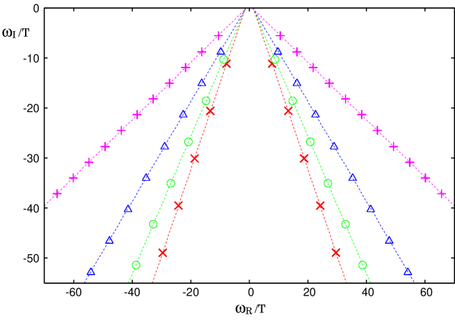
Figure 1: QN frequencies for D$1$($\times$), D$2$($\circ$), D$3$($\triangle$) and D$4$-branes($+$). Each straight line is determined by the least-square fitting.

As is apparent from Fig.1, the QN frequencies for each $p$ are distributed on the straight line. The QN frequencies are approximately given by the modes $n$ ($n=0,1,2,\cdots$) of the formula below:

$$\hat{\omega}_{n}/\hat{T}=\alpha_{p}~{}n+\beta_{p}~{},$$ (39)

where

$$\alpha_{p}=\begin{cases}5.45-9.43\,i&\text{for~{}~{}}p=1\cr 6.00-8.23\,i&\text{for~{}~{}}p=2\cr 6.32-6.29\,i&\text{for~{}~{}}p=3\cr 5.52-3.16\,i&\text{for~{}~{}}p=4\cr\end{cases}~{}, \beta_{p}=\begin{cases}7.80-11.17\,i&\text{for~{}~{}}p=1\cr 8.76-10.27\,i&\text{for~{}~{}}p=2\cr 9.88-8.66\,i&\text{for~{}~{}}p=3\cr 10.66-5.53\,i&\text{for~{}~{}}p=4\cr\end{cases}~{}.$$ (40)

This property that the QN frequencies are approximately evenly spaced with $n$ is numerically observed for the scalar, vector, and gravitational perturbations on the ${\rm SAdS}_{4}$ black holes CKL and on the ${\rm SAdS}_{5}$ black holes ref:Starinets ; ref:NunezStarinets ; ref:KovtunStarinets . The property is analytically shown for a minimally coupled massive scalar ref:MusiriSiopsis and the vector perturbations ref:NunezStarinets on the ${\rm SAdS}_{5}$ black hole. For highly-overtone QN frequencies, one can make a comprehensive research analytically ref:NatarioSchiappa . However, its origin and significance are far from obvious.

IV.1 $p=1$ and $p=4$

For both $p=1$ and $p=4$, the dilaton gravity action (20) is simply written by

$$S\sim\int d^{p+2}x~{}\sqrt{-\underline{g}}~{}e^{2a\phi}~{}\Big{(}\underline{R}-2\Lambda\Big{)}~{}.$$ (41)

So, under the metric ansatz:

$$ds_{(p+3)}^{2}=\underline{ds}^{2}+\left(\frac{5-p}{2}\right)^{2}\left(\frac{e^{\phi}}{g_{s}}\right)^{\frac{4(5-p)}{(7-p)(p-3)}}dz^{2}$$ (42)

one can embed the $(p+2)$-dimensional action (41) into the $(p+3)$-dimensional action:

$$S\sim\int d^{p+3}x\sqrt{-g_{(p+3)}}~{}\Big{(}~{}{}^{(p+3)}\!R-2\Lambda~{}\Big{)}~{}.$$ (43)

For $p=4$, the embedding can be understood as the M-theory embedding (M5-brane) of the D4-brane, and this M5-brane reduces to the planar ${\rm SAdS}_{7}$ black hole (in the near-horizon limit).

For $p=1$, D1-brane does not have a M-theory embedding because it is a type IIB object. However, various dualities relate the D1-brane to the M2-brane. Under the four-dimensional pure gravity theory, the metric (42) becomes

$$ds^{2}=-(\tilde{r}^{2}-\tilde{r_{0}}^{3}/\tilde{r})dt^{2}+(\tilde{r}^{2}-\tilde{r_{0}}^{3}/\tilde{r})^{-1}dr^{2}+\tilde{r}^{2}(dx^{2}+dz^{2}),$$ (44)

where we set $l=1$ for simplicity. This metric corresponds to the planar ${\rm SAdS}_{4}$ metric. So, one can compare our $p=1$ results with the ones for the ${\rm SAdS}_{4}$ in the large black hole limit. Table 2 is the comparison with the results by Cardoso, et.al. CKL corresponding to the $\ell=2$ gravitational perturbations (even parity) of a large ${\rm SAdS}_{4}$ black hole ($l=1$ and $\tilde{r}_{0}=100$). Their results are normalized with respect to the Hawking temperature $T=(q/4\pi)\,(\tilde{r}_{0}/l^{2})$. One can easily see that our results agree well with the ${\rm SAdS}_{4}$ results in the large black hole limit.

	Ours		Cardoso, et.al
Mode	$\hat{\omega}_{R}/\hat{T}$	$\hat{\omega}_{I}/\hat{T}$	$\omega_{R}/T$	$\omega_{I}/T$
$0$	07.747	-11.158	07.748	-11.157
$1$	13.242	-20.594	13.244	-20.591
$2$	18.700	-30.023	18.703	-30.020
$3$	24.149	-39.450	24.153	-39.446

Table 2: QN frequencies corresponding to $\ell=2$ gravitational perturbations (even parity) of a large Schwarzschild-AdS black hole with $\tilde{r}_{0}=100$ and $l=1$.

IV.2 $p=2$

On the other hand, the $p=2$ case is not related to a higher-dimensional SAdS, contrary to the $p=1$ and $p=4$ cases. Obviously, one can always embed type IIA objects into M-theory. However, the resulting geometries are not SAdS black holes, and QN frequencies for such geometries are unknown.

The D2-brane is embedded as a M2-brane, but the embedding of the geometry (6) is not the ${\rm SAdS}_{4}$. This is because the embedding corresponds not to the standard M2-brane, but rather corresponds to the so-called “smeared M2-brane.” In a sense, we have obtained QN frequencies of the “smeared M2-brane” via the D2-brane.

Even the smeared M2-brane description is not valid at lower energy. The smeared M2-brane becomes unstable at lower energy due to the Gregory-Laflamme instability and decays into the M2-brane on a circle. Then, the ${\rm SAdS}_{4}$ calculation suffices for such a small black hole Itzhaki:1998dd .

IV.3 Sensibility on the boundary condition

We placed the Dirichlet condition at infinity to compute QN frequencies. However, supergravity description often breaks down at infinity. So, strictly speaking, one must place an ultraviolet cutoff and put a boundary condition at the large finite radius. Here, we discuss how such a boundary condition may change our results.

First of all, it is not clear what boundary condition one must impose. The out-going wave certainly leaks out to the asymptotic infinity. So, a simple Dirichlet condition at the cutoff does not suffice. However, appropriate boundary condition is not clear, so here we use a Dirichlet boundary condition for illustration to see if our results are sensitive to the boundary condition.

Figure 2 is the result of QN frequencies (for $p=1$) by imposing the Dirichlet condition at various radii $x_{b}=(r_{0}/r_{b})^{2}$. (Here, $r_{b}$ is the location of the boundary condition in the original D-brane coordinate $r$.) As the figure shows, the result begins to converge for a sufficiently large boundary radius (say, $x_{b}<0.02$ or $r_{b}>r_{0}/\sqrt{0.02}$). For the boundary condition placed in the plateau region, the result is effectively the same as the one with the boundary condition at infinity. In other words, the result is insensitive to the boundary condition.

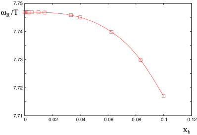
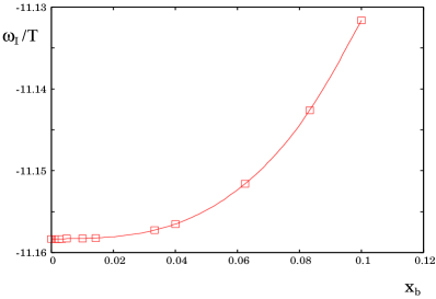
Figure 2: The dependence of the lowest QN frequency on the location of the boundary condition $x_{b}$. The left figure (right figure) is the real (imaginary) part of the QN frequency.

Let us reinterpret the result in terms of SYM variables. The D1 description is valid for $g_{YM}N^{1/6}\ll r/l_{s}^{2}\ll(g_{YM}^{2}N)^{1/2}$ in SYM variables. Actually, gravity description is valid even inside the infrared cutoff. The type IIB fundamental string description takes over (via type IIB S-duality), but the gravity computation is the same as the D1 case. Supergravity descriptions are valid as long as $g_{YM}\ll r/l_{s}^{2}\ll(g_{YM}^{2}N)^{1/2}$.

The theory has two independent parameters $g_{YM}$ and $N$. The infrared cutoff can be controlled by $g_{YM}$ whereas the ultraviolet cutoff can be controlled by $N$. Thus, the condition $x_{b}<0.02$ must be satisfied for a large enough $N$. This is indeed true.

In order for the QN frequency to be insensitive to the boundary condition, $r_{b}$ must lie within this region. This implies $g_{YM}\ll r_{0}/l_{s}^{2}\ll(0.02g_{YM}^{2}N)^{1/2}$. This condition has a solution if $N\gg 50$.

V Summary

We have computed the scalar QN frequencies for asymptotically AdS black holes (in appropriate frame), which correspond to the decoupling limit of nonextreme D$p$-branes (for $p<5$). We consider the translationally invariant perturbations along the branes. The dual gauge theory is described by $(p+1)$-dimensional super-Yang-Mills theories at finite temperature.

As discussed in Sect. IV, one can embed the system into higher dimensions for $p=1$ and $p=4$. Then, the bulk geometries become just SAdS black holes. Thus, these cases can be reproduced by QN frequency calculations of standard SAdS black holes. (However, they correspond to different region of the validity, so one must be careful to its interpretation. For example, the $p=4$ case reduces to the M5-brane, but this must be interpreted as the recovery of conformality at high energy.) This gives a nice check of our approach since our perturbation is more involved compared with the standard cases. (Only the minimally-coupled test scalar field is often considered to calculate QN frequencies.) We explicitly checked that our results coincide with the SAdS results.

On the other hand, $p=2$ case is not obtained from higher dimensional SAdS black hole. Thus, the embedding of the $p=2$ case does not help to simplify the calculation. The fact that QN frequencies are evenly spaced had been observed for pure gravity black holes. Our $p=2$ result may indicate that this is true even for some dilatonic AdS black holes.

It is difficult to calculate the thermalization time scale in the gauge theory. But Ref. HoHu pointed out that the time scale is likely to be independent of the ’t Hooft coupling. A free field theory never thermalizes and at weak coupling the time scale should be very long. So, clearly the time scale depends on the coupling at weak coupling. However, in the strong coupling, the relaxation time scale is expected to be the order of the thermal wavelength.

In the dual supergravity description, this means that the QN frequencies depend only on the Hawking temperature. This expectation is indeed true for SAdS black holes HoHu , and we found that it is also true for D$p$-branes. (Table 1 shows that QN frequencies are linear in temperature.)

Finite temperature gauge/gravity dualities deserve further study. To qualitatively check the duality, one wishes to check the time scale in the dual theory. Currently, it is difficult to calculate the time scale in gauge theories. Such a calculation has not been carried out even in the SAdS cases. But gauge theory understanding is essential to solve the long-standing puzzles such as the singularity problem, the information paradox, and the Gregory-Laflamme instability.

Note added: After this work was completed, we were informed about work by Iizuka, Kabat, Lifschytz, and Lowe Iizuka:2003ad , where they also computed QN frequencies for nonextreme D$p$-branes. The differences from our paper are as follows: (1) We computed not only the lowest modes, but also higher modes as well. As a result, we are able to see how eigenvalues are distributed in the complex plane. (2) The perturbation considered in the paper eventually becomes the same as ours. However, they regarded the perturbation simply as a minimally-coupled test scalar field, whereas we derived the equation from a combination of the gravitational and dilaton perturbations, which is part of type II spectrum in those backgrounds. (3) We also consider the validity of supergravity descriptions.

We would like to thank D. Kabat for communicating their results.

*

Appendix A Review of Quasinormal Modes

We briefly review quasinormal modes (for a comprehensive review, see ref:KokkotasSchmidt ).

Let us consider the initial-value problem of a linear wave equation for a scalar field $\Phi$

$$\big{(}-\square+V(x)~{}\big{)}\,\Phi(x)=0~{}.$$ (45)

As is well-known, we can formally solve the initial-value problem using the retarded Green function $G_{R}$ as ref:MorseFeshbach

$$\Phi(x)=\int_{\Sigma_{0}}d\Sigma(z)~{}\Big{[}~{}\Big{(}n^{\mu}\partial^{z}_{\mu}\,G_{R}(x\,;z)\Big{)}~{}\Phi(z)-G_{R}(x\,;z)~{}\Big{(}n^{\mu}\partial^{z}_{\mu}\,\Phi(z)\Big{)}~{}\Big{]}~{},$$ (46)

where $d\Sigma(z)$ is the infinitesimal surface element of the initial surface $\Sigma_{0}$ and $n^{\mu}$ is future-directed unit normal vector to $\Sigma_{0}$.

The retarded Green function $G_{R}(x\,;z)$ in $(d+1)$-dimensional spacetime is the solution of the inhomogeneous wave equation

$$\big{(}-\square_{x}+V(x)~{}\big{)}\,G_{R}(x\,;z)=-\delta^{(d+1)}(x-z)/\sqrt{-g(x)}~{},$$ (47)

satisfying the causal condition, $G_{R}(x\,;z)=0$ for $x\notin J^{+}(z)$.

For static spacetimes, $ds^{2}=N^{2}(\bm{\bm{x}})\,\big{(}-dt^{2}+\gamma_{ij}(\bm{\bm{x}})dx^{i}dx^{j}\,\big{)}$, so the Green function is time-translationally invariant, $G_{R}(x\,;z)=:G_{R}(t,\bm{\bm{x}}\,;\tau,\bm{\bm{z}})=G_{R}(t-\tau,\bm{\bm{x}}\,;0,\bm{\bm{z}})$, and it is convenient to use the “frequency-domain Green function”  $\tilde{g}_{R}$ defined by

$$\tilde{g}_{R}(\bm{\bm{x}}\,;\bm{\bm{z}}|s)=\left[~{}N(\bm{\bm{x}})~{}N(\bm{\bm{z}})~{}\right]^{(d-1)/2}~{}\int^{\infty}_{0^{-}}dt~{}e^{-s\,t}~{}G_{R}(t,\bm{\bm{x}}\,;0,\bm{\bm{z}})~{},$$ (48)

which is simply the Laplace transform of $G_{R}$ (with the weight $N^{(d-1)/2}$ inserted for convenience). If there exists such a Laplace transform $\tilde{g}_{R}$, an abscissa of convergence $\sigma$ exists and $\tilde{g}_{R}$ is well-defined for $\Re(s)>\sigma$. Then, $\tilde{g}_{R}$ satisfies the equation,

$$\left[~{}s^{2}-\Delta_{\bm{\bm{x}}}+\cdots~{}\right]\,\tilde{g}_{R}(\bm{\bm{x}}\,;\bm{\bm{z}}|s)=-\delta^{(d)}(\bm{\bm{x}}-\bm{\bm{z}})/\sqrt{\gamma(\bm{\bm{x}})}~{},$$ (49)

where $\Delta$ is the Laplacian with respect to the metric $\gamma_{ij}$ and the dots denote the terms by the “effective potential”. After solving Eq.(49) with a suitable boundary condition, $G_{R}$ is obtained by

$$G_{R}(t,\bm{\bm{x}}\,;0,\bm{\bm{z}})=\left[~{}N(\bm{\bm{x}})~{}N(\bm{\bm{z}})~{}\right]^{(1-d)/2}~{}\int^{\sigma+i\,\infty}_{\sigma-i\,\infty}\frac{ds}{2\pi\,i}~{}e^{s\,t}~{}\tilde{g}_{R}(\bm{\bm{x}}\,;\bm{\bm{z}}|s)~{}.$$ (50)

One can define $\tilde{g}_{R}$ for $\Re(s)<\sigma$ by the analytical continuation from $\Re(s)>\sigma$. Provided that $|s\,e^{st}\,\tilde{g}_{R}|\xrightarrow{|s|\rightarrow\infty}0$ for $\Re(s)<\sigma$, the contribution to $G_{R}$ in Eq.(50) comes from the singularities of $\tilde{g}_{R}$ in $\Re(s)<\sigma$. The pole singularities of $\tilde{g}_{R}$, $\{s_{n}\}_{n=0,1,2,\cdots}$, contribute to $G_{R}$ as

$$G_{R}(t,\bm{\bm{x}}\,;\tau,\bm{\bm{z}})=\left[~{}N(\bm{\bm{x}})~{}N(\bm{\bm{z}})~{}\right]^{(1-d)/2}~{}\sum_{n}e^{s_{n}\,(t-\tau)}~{}\text{Res}\big{[}~{}\tilde{g}_{R}(\bm{\bm{x}}\,;\bm{\bm{z}}|s)\,;\,s_{n}~{}\big{]}+\cdots~{},$$ (51)

and the corresponding frequency for each pole $\omega_{n}=i\,s_{n}$ ($\Im(\omega_{n})<\sigma$) is called a quasinormal frequency. So, a quasinormal frequency is given by a pole of the retarded Green function in the frequency domain, $\tilde{g}_{R}(\bm{\bm{x}}\,;\bm{\bm{z}}|s)$.

In order to obtain $\tilde{g}_{R}$, one must pay attention to the boundary conditions for Eq.(49). We consider two cases separately.

1. For asymptotically flat black hole spacetimes, there are two asymptotic regions, the near-horizon region and spatial infinity. Equation (49) often has simple forms in these regions:

   $$\big{(}s^{2}-\partial_{r_{*}}^{2}\big{)}\,\tilde{g}_{R}(\bm{\bm{x}}\,;\bm{\bm{z}}|s)\sim 0~{},$$ (52)

   where we consider a massless scalar field for simplicity. The tortoise coordinate of $x$, $r_{*}$, is defined such that the spatial infinity (the horizon) corresponds to $r_{*}\rightarrow\infty~{}(-\infty)$. There are two independent solutions $e^{\pm s\,r_{*}}$ in each asymptotic region.

   Recalling that $\tilde{g}_{R}$ for $\Re(s)<\sigma$ is given by the analytic continuation from $\Re(s)>\sigma$, we first consider the boundary conditions of $\tilde{g}_{R}$ for $\Re(s)>\sigma$. Since diverging solutions are unphysical, $\tilde{g}_{R}$ for $\Re(s)>\sigma$ should behave as

   $$\tilde{g}_{R}(\bm{\bm{x}}\,;\bm{\bm{z}}|s)\rightarrow e^{s\,r_{*}}\hskip 8.5359pt(e^{-s\,r_{*}}) \text{~{}~{}for~{}~{}}r_{*}\rightarrow-\infty\hskip 8.5359pt(\infty)~{},$$ (53)

   so that

   $$G_{R}(t,\bm{\bm{x}}\,;0,\bm{\bm{z}})\sim e^{st}~{}\tilde{g}_{R}(\bm{\bm{x}}\,;\bm{\bm{z}}|s)\rightarrow e^{s\,(t+r_{*})}\hskip 8.5359pt(e^{s\,(t-r_{*})}) \text{~{}~{}for~{}~{}}r_{*}\rightarrow-\infty\hskip 8.5359pt(\infty)~{}.$$ (54)

   This means that the appropriate boundary conditions for the retarded Green function $G_{R}$ in this case are a purely ingoing wave near the horizon and an outgoing wave at the infinity. Since $\tilde{g}_{R}$ for $\Re(s)<\sigma$ is defined by the analytical continuation from $\Re(s)>\sigma$, $\tilde{g}_{R}$ for $\Re(s)<\sigma$ also satisfies the same boundary conditions (53), in spite of the diverging behavior.

2. For asymptotically AdS black hole spacetimes, the tortoise coordinate $\eta_{*}$ is defined such that the null infinity (the horizon) corresponds to $\eta_{*}\rightarrow 0$ ($-\infty$). Although Eq.(49) has the same form as Eq.(52) near the horizon, Eq.(49) has a different form near the null infinity,

   $$\left(-\partial_{\eta_{*}}^{2}+C/\eta_{*}^{2}\right)\tilde{g}_{R}(\bm{\bm{x}}\,;\bm{\bm{z}}|s)\sim 0 \text{for~{}~{}}\eta_{*}\rightarrow 0~{},$$ (55)

   where $C$ is a positive constant. Thus, for $\eta_{*}\sim 0$, we obtain $\tilde{g}_{R}(\bm{\bm{x}}\,;\bm{\bm{z}}|s)\sim\eta_{*}^{1/2\pm\sqrt{C+1/4}}$ or $G_{R}(t,\bm{\bm{x}}\,;0,\bm{\bm{z}})\sim\eta_{*}^{d/2\pm\sqrt{C+1/4}}=:\eta_{*}^{\Delta_{\pm}}$, where we use $N^{(1-d)/2}(\bm{\bm{x}})\propto\eta_{*}^{(d-1)/2}$ for $\eta_{*}\sim 0$. Since we have $\Delta_{-}<0<\Delta_{+}$ in many cases, we henceforth assume $\Delta_{-}<0<\Delta_{+}$.

   Again, we first consider $\tilde{g}_{R}$ for $\Re(s)>\sigma$. Since diverging solutions are physically unacceptable, $\tilde{g}_{R}$ for $\Re(s)>\sigma$ should behave as

   $$\tilde{g}_{R}(\bm{\bm{x}}\,;\bm{\bm{z}}|s)\rightarrow\begin{cases}e^{s\,\eta_{*}}&\text{~{}~{}for~{}~{}}\eta_{*}\rightarrow-\infty\\ \eta_{*}^{1/2+\sqrt{C+1/4}}&\text{~{}~{}for~{}~{}}\eta_{*}\rightarrow 0\end{cases}~{},$$ (56)

   so that

   $$G_{R}(t,\bm{\bm{x}}\,;0,\bm{\bm{z}})\sim e^{st}~{}\tilde{g}_{R}(\bm{\bm{x}}\,;\bm{\bm{z}}|s)\rightarrow\begin{cases}e^{s\,(t+\eta_{*})}&\text{~{}~{}for~{}~{}}\eta_{*}\rightarrow-\infty\\ e^{s\,t}~{}\eta_{*}^{\Delta_{+}}&\text{~{}~{}for~{}~{}}\eta_{*}\rightarrow 0\end{cases}~{}.$$ (57)

   We should set the same boundary conditions (56) to $\tilde{g}_{R}$ for $\Re(s)<\sigma$ because $\tilde{g}_{R}$ for $\Re(s)<\sigma$ is defined by the analytical continuation from $\Re(s)>\sigma$.

To summarize, quasinormal frequencies are obtained by finding the poles of $\tilde{g}_{R}$ satisfying Eq.(49) with the boundary conditions. However, it is easy to show that, for a pole of $\tilde{g}_{R}$, $s_{n}$, there exists an eigenmode $\tilde{\phi}_{n}(\bm{\bm{x}})$ of the homogeneous equation of Eq.(49)

$$\left(s^{2}-\Delta+\cdots\right)\,\tilde{\phi}_{n}(\bm{\bm{x}})=0~{},$$ (58)

which satisfies the boundary conditions (53) for asymptotically flat black hole spacetimes ref:KokkotasSchmidt , and (56) for asymptotically AdS black hole spacetimes. Thus, in practice, one can also find the quasinormal frequencies by solving this eigenvalue problem. In the main text, we solve this eigenvalue problem (58) with the boundary conditions (56).

References

- (1) E. Witten, Adv. Theor. Math. Phys. 2, 505 (1998), “Anti-de Sitter space, thermal phase transition, and confinement in gauge theories,” [arXiv:hep-th/9803131].
- (2) P. Kraus, H. Ooguri and S. Shenker, Phys. Rev. D67, 124022 (2003), “Inside the horizon with AdS/CFT,” [arXiv:hep-th/0212277].
- (3) G. Festuccia and Hong Liu, hep-th/0506202, “Excursion beyond the horizon: Black hole singularities in Yang-Mills theories.”
- (4) J. M. Maldacena, J. High Energy Phys. 04 (2003) 021, “Eternal black holes in Anti-de-Sitter,” [arXiv:hep-th/0106112].
- (5) S. W. Hawking, hep-th/0507171, “Information loss in black holes.”
- (6) R. Gregory and R. Laflamme, Phys. Rev. Lett. 70, 2837 (1993), “Black strings and p-branes are unstable,” [arXiv:hep-th/9301052]; Nucl. Phys. B 428, 399 (1994), “The Instability of charged black strings and p-branes,” [arXiv:hep-th/9404071]; Phys. Rev. D51, R305 (1995), “Evidence for stability of extremal black p-branes,” [arXiv:hep-th/9410050].
- (7) O. Aharony, J. Marsano, S. Minwalla and T. Wiseman, Class. Quant. Grav. 21, 5169 (2004), “Black hole - black string phase transitions in thermal 1+1 dimensional supersymmetric Yang-Mills theory on a circle,” [arXiv:hep-th/0406210].
- (8) S. W. Hawking and D. N. Page, Commun. Math. Phys. 87, 577 (1983), “Thermodynamics Of Black Holes In Anti-De Sitter Space.”
- (9) I. R. Klebanov and M. J. Strassler, J. High Energy Phys. 08 (2000) 052, “Supergravity and a confining gauge theory: Duality cascades and SB-resolution of naked singularities,” [arXiv:hep-th/0007191].
- (10) J. Polchinski and M. J. Strassler, hep-th/0003136, “The string dual of a confining four-dimensional gauge theory.”
- (11) N. Itzhaki, J. M. Maldacena, J. Sonnenschein and S. Yankielowicz, Phys. Rev. D58, 046004 (1998), “Supergravity and the large N limit of theories with sixteen supercharges,” [arXiv:hep-th/9802042].
- (12) A. Brandhuber, N. Itzhaki, J. Sonnenschein and S. Yankielowicz, J. High Energy Phys. 06 (1998) 001, “Wilson loops, confinement, and phase transitions in large N gauge theories from supergravity,” [arXiv:hep-th/9803263].
- (13) Y. Sekino and T. Yoneya, Nucl. Phys. B 570, 174 (2000), “Generalized AdS-CFT correspondence for matrix theory in the large N limit,” [arXiv:hep-th/9907029].
- (14) G. T. Horowitz and V. E. Hubeny, Phys. Rev. D62, 024027 (2000), “Quasinormal modes of AdS black holes and the approach to thermal equilibrium,” [arXiv:hep-th/9909056].
- (15) I. G. Moss and J. P. Norman, Class. Quant. Grav. 19, 2323 (2002), “Gravitational quasinormal modes for Anti-de Sitter black holes,” [arXiv:gr-qc/0201016].
- (16) E. Berti, K. D. Kokkotas, Phys. Rev. D67, 064020 (2003), “Quasinormal modes of Reissner-Nordström-anti-de Sitter black holes: scalar, electromagnetic and gravitational perturbations”, [arXiv:gr-qc/0301052].
- (17) V. Cardoso, R. Konoplya, and J. P. S. Lemos, Phys. Rev. D68, 044024 (2003), “Quasi-normal frequencies of Schwarzschild black holes in anti-de Sitter spacetime: A complete study of the overtome asymptotic behavior,” [arXiv:gr-qc/0305037].
- (18) R. A. Konoplya, Phys. Rev. D68, 124017 (2003), “Gravitational quasinormal radiation of higher-dimensional black holes,” [arXiv:hep-th/0309030].
- (19) S. Musiri and G. Siopsis, Phys. Lett. B 563, 102 (2003), “Quasinormal modes of large AdS black holes”, [arXiv:hep-th/0301081]; Phys. Lett. B 576, 309 (2003), “Asymptotic form of quasi-normal modes of large AdS black holes”, [arXiv:hep-th/0308196].
- (20) P. Benincasa, A. Buchel and A. O. Starinets, hep-th/0507026, “Sound waves in strongly coupled non-conformal gauge theory plasma,” [arXiv:hep-th/0507026].
- (21) G. Policastro, D. T. Son and A. O. Starinets, J. High Energy Phys. 09 (2002) 043, “From AdS/CFT correspondence to hydrodynamics,” [arXiv:hep-th/0205052].
- (22) A.O. Starinets, Phys. Rev. D66, 124013 (2002), “Quasinormal modes of near extremal black branes”, [arXiv:hep-th/0207133].
- (23) A. Núñez and A.O. Starinets, Phys. Rev. D67, 124013 (2003), “AdS/CFT correspondence, quasinormal modes, and thermal correlators in supersymmetric Yang-Mills theory”, [arXiv:hep-th/0302026].
- (24) P.K. Kovtun and A.O. Starinets, hep-th/0506184, “Quasinormal modes and holography.”
- (25) J. Polchinski, String theory. Vol. 2: Superstring theory and beyond, (Cambridge University Press, Cambridge, 1998).
- (26) H. J. Boonstra, K. Skenderis, P. K. Townsend, J. High Energy Phys. 01 (1999) 003, “The domain-wall/QFT correspondence,” [arXiv:hep-th/9807137].
- (27) H. Kodama and M. Sasaki, Prog. Theor. Phys. Suppl. 78, 1 (1984), “Cosmological Perturbation Theory.”
- (28) E. W. Leaver, Phys. Rev. D41, 2986 (1990), “Quasinormal modes of Reissner-Nordström black holes.”
- (29) V. Cardoso, J. Natario, and R. Schiappa, J. Math. Phys. 45, 4698 (2004), “Asymptotic Quasinormal Frequencies for Black Holes in Non-Asymptotically Flat Spacetimes,”[arXiv:hep-th/0403132]; J. Natario and R. Schiappa, hep-th/0411267, “On the Classification of Asymptotic Quasinormal Frequencies for -Dimensional Black Holes and Quantum Gravity.”
- (30) N. Iizuka, D. Kabat, G. Lifschytz and D. A. Lowe, Phys. Rev. D68, 084021 (2003), “Stretched horizons, quasiparticles and quasinormal modes,” [arXiv:hep-th/0306209].
- (31) K.D. Kokkotas and B.G. Schmidt, “Quasi-Normal Modes of Stars and Black Holes,”(August, 1999), [Article in Online Journal Living Reviews in Relativity]: http://relativity.livingreviews.org/Articles/lrr-1999-2/index.html.
- (32) P.M. Morse and H. Feshbach, Methods of Theoretical Physics, (McGraw-Hill. New York, 1953).