Moduli Stabilization in String Gas Compactification

Abstract

We investigate the moduli stabilization in string gas compactification. We first present a numerical evidence showing the stability of the radion and the dilaton. To understand this numerical result, we construct the 4-dimensional effective action by taking into account T-duality. It turns out that the dilaton is actually marginally stable. When the moduli other than the dilaton is stabilized at the self-dual point, the potential for the dilaton disappears and then the dilaton is stabilized due to the hubble damping. In order to investigate if this mechanism works in more general cases, we analyze the stability of $T_{2}\otimes T_{2}\otimes T_{2}$ compactification in the context of massless string gas cosmology. We found that the volume moduli, the shape moduli, and the flux moduli are stabilized at the self dual point in the moduli space. Thus, it is proved that this simple compactification model is stable.

I Introduction

It is widely believed that the superstring theory is the most promising candidate for the quantum theory of gravity. The most attractive feature of the superstring theory is the existence of the target space duality ( T-duality ) Kikkawa:1984cp . It is T-duality that implies the minimal length scale, i.e. the string length scale $\ell_{s}$ (we take the unit $\ell_{s}=1$ throughout this paper). Thus, there is a possibility to avoid the cosmological initial singularity in the superstring theory. Another feature of the superstring theory is the presence of extra-dimensions. Therefore, it is inevitable to study the higher-dimensional cosmology and explain how 4-dimensional large external space emerges. Brandenberger and Vafa proposed an interesting cosmological scenario Brandenberger:1988aj ; Tseytlin:1991xk (see also previous works Nishimura:1986wp ; Matsuo:1986es ; Kripfganz:1987rh ). They argued the avoidance of the cosmological singularity due to T-duality and proposed a mechanism how only 3 spatial dimensions become large through the annihilation of winding modes (see also Easther:2002mi ; Easther:2004sd concerning this point). Recent developments of D-brane physics stimulates the study of string gas or brane gas scenario Alexander:2000xv ; Easson:2001fy ; Boehm:2002bm ; Watson:2002nx ; Campos:2003gj ; Bassett:2003ck ; Easson:2005ug ; Kaya:2005qm .

Because this idea is so attractive, it is important to clarify the issue of moduli stabilization in this scenario. The purpose of this paper is to reveal to what extent the moduli can be stabilized in the scenario of Brandenberger and Vafa.

Historically, Watson and Brandenberger first demonstrated the stability of the radion but in their work the dilaton runs logarithmically Watson:2003gf ; Berndsen:2004tj . The 4-dimensional effective action is also obtained and concluded neither the dilaton nor the radion can be stabilized except for 5-dimensional case Battefeld:2004xw . The effects of inhomogeneous perturbations are investigated and it is shown that they do not affect the stability of the radion Watson:2003uw . The importance of the massless string modes are recently recognized Watson:2004aq ; Patil:2004zp ; Patil:2005fi . The effects of D-string gas is also studied Patil:2005nm . However, all of the previous analysis are restricted to the special subspace of the moduli space and the role of T-duality has not been fully explored. In this paper, we investigate moduli stabilization in the string gas compactification generally with focusing on T-duality.

The organization of this paper is as follows. In sec.II, we review T-duality in the low energy effective action of string theory. We also present a string gas model as the T-duality invariant matter. In sec.III, we present the numerical calculations of the simplest case which show the stability of the radion and the dilaton. In sec.IV, we obtain the T-duality invariant 4-dimensional effective action and clarify why the dilaton is stabilized in our numerical results. In sec.V, using the 4-dimensional effective action, we show the stability of $T_{2}\otimes T_{2}\otimes T_{2}$ compactification. The final section is devoted to the conclusion.

II T-duality in Cosmology

Here, we would like to review T-duality in string theory with focusing on its relation to cosmology. In the low energy effective action of string theory, there exists the $O(6,6,{\bf R})$ symmetry which includes the T-duality symmetry $O(6,6,{\bf Z})$ as a special case Gasperini:1991ak ; Giveon:1994fu ; Lidsey:1999mc ; Gasperini:2002bn . In the full string theory, $O(6,6,{\bf R})$ symmetry cease to exist. However, the T-duality symmetry $O(6,6,{\bf Z})$ remains. In fact, in the case of a string propagating in constant background fields, the T-duality symmetry $O(6,6,{\bf Z})$ exists in the mass spectrum of a quantum string. In the cosmological background, we do not know exact spectrum. Here, we treat the gas of strings as test objects and take the metric in a self-consistent manner. It is usual to do so in cosmology.

II.1 T-duality in Low Energy Effective Action

The bosonic part of the low energy effective action of the superstring theory takes the following form

$$S=\frac{1}{2\kappa^{2}}\int d^{10}x\sqrt{-G}e^{-2\phi}\left[\overset{(10)}{R}+4(\nabla\phi)^{2}-\frac{1}{12}H^{2}\right]\ ,$$ (1)

where $G_{AB}$ and $\phi$ denote the 10-dimensional metric with $A,B=0,1,\cdots,9$ and the dilaton, respectively. Here, we used the notation $(\nabla\phi)^{2}=\partial^{A}\phi\partial_{A}\phi$ and $H=dB$ is the field strength of the anti-symmetric tensor field $B_{AB}$. We also defined the 10-dimensional gravitational coupling constant $\kappa$.

We assume the 4-dimensions are selected by the Brandenberger-Vafa mechanism. Hence, we consider the cosmological ansatz for the metric:

$$ds^{2}=g_{\mu\nu}(x^{\mu})dx^{\mu}dx^{\nu}+\gamma_{ab}(x^{\mu})dy^{a}dy^{b}\ ,$$ (2)

where $g_{\mu\nu}$ is the metric of 4-dimensional external spacetime and $\gamma_{ab}$ is the metric of the internal 6-dimensional compact space. Here, both metric are assumed to depend only on 4-dimensional coordinates $x^{\mu}$. This means the internal space is flat with respect to $y^{a}$ . It is convenient to define shifted dilaton $\bar{\phi}$ by

$$\sqrt{\gamma}e^{-2\phi}\equiv e^{-2\bar{\phi}}\ .$$ (3)

Now, we define the 6$\times$6 matrix $(\Gamma)_{ab}=\gamma_{ab}$ in terms of the internal space components of the metric. We assume the anti-symmetric field $B_{AB}$ exists only in the internal space defined by the 6$\times$6 matrix, $(B)_{ab}=B_{ab}$ depending only on 4-dimensional coordinate $x^{\mu}$. Then the action can be set into a more compact form by using the 12 $\times$ 12 matrix $Q$:

$$Q=\left(\begin{array}[]{ll}\Gamma^{-1}&\quad-\Gamma^{-1}B\\ B\Gamma^{-1}&\quad\Gamma-B\Gamma^{-1}B\end{array}\right)$$ (6)

which satisfies a symmetric matrix element of the pseudo- orthogonal $O(6,6,{\bf R})$ group, since

$$Q^{T}\eta Q=\eta\ ,\quad Q^{T}=Q\ ,$$ (7)

for any $B$ and $\Gamma$. Here, $\eta$ consists of the unit 6-dimensional matrix $I$,

$$\eta=\left(\begin{array}[]{cc}0&I\\ I&0\end{array}\right)\ .$$ (10)

Using the metric (2) and the variables (3) and (4), the action can be written as

$$S=\frac{V_{6}}{2\kappa^{2}}\int d^{4}xe^{-2\bar{\phi}}\left[R+4(\partial\bar{\phi})^{2}+\frac{1}{8}{\rm Tr}\partial^{\mu}{Q}\partial_{\mu}Q^{-1}\right]\ ,$$ (11)

where $V_{6}$ is the coordinate volume of the internal space and $R$ is the 4-dimensional scalar curvature. Here, $(\partial\bar{\phi})^{2}$ represents $\partial^{\mu}\bar{\phi}\partial_{\mu}\bar{\phi}$ and ${\rm Tr}$ denotes the trace of the matrix. One can see the action is invariant under $O(6,6,{\bf R})$ transformation

$$Q\rightarrow\tilde{Q}=\Lambda^{T}Q\Lambda\ ,$$ (12)

where $\Lambda$ is the $12\times 12$ matrix satisfying $\Lambda^{T}\eta\Lambda=\eta$. Note that the shifted dilaton is invariant under this $O(6,6,{\bf R})$ transformation $\bar{\phi}\rightarrow\bar{\phi}$. The special $O(6,6,{\bf R})$ transformation represented by $\Lambda=\eta$ belongs to T-duality transformation. More explicitly Eq. (12) gives,

$$\tilde{\Gamma} = \left(\Gamma-B\gamma^{-1}B\right)^{-1}$$ (13)

$$\tilde{B} = -\Gamma^{-1}B\left(\Gamma-B\Gamma^{-1}B\right)^{-1}$$ (14)

When we set $B=0$, this corresponds to an inversion of the internal space matrix, $\tilde{\Gamma}=\Gamma^{-1}$. So far, we have seen only the kinetic part. It is interesting to see if the potential energy for the moduli can be induced by the string gas. If yes, because of T-duality, one can expect the moduli in the internal space are stabilized at the self-dual point, $\tilde{\Gamma}=\Gamma$ and $\tilde{B}=B$. This is the subject of the next subsection.

II.2 T-duality Invariant String Gas

Let us consider a closed string in the constant background field $g_{\mu\nu},\gamma_{ab},B_{ab}$. The action for the string with the position $X^{A}$ is given by the nonlinear sigma model,

$$S = -\frac{1}{4\pi}\int d\sigma d\tau\left[G_{AB}\partial^{\cal M}X^{A}\partial_{\cal M}X^{B}\right.$$ (15)

$$\qquad\qquad\qquad\qquad\quad\left.+\epsilon^{\cal MN}B_{AB}\partial_{\cal M}X^{A}\partial_{\cal N}X^{B}\right]$$

$$\equiv -\frac{1}{4\pi\alpha^{\prime}}\int d\sigma d\tau{\cal L}$$

where indices $\{\cal{M,N,\cdots}\}$ are used for tensors on a 2-dimensional world-sheet which can be described in terms of two parameters $X^{A}(\tau,\sigma)$. Defining variables

$$P^{\tau}_{A} \equiv \frac{\partial\cal L}{\partial\dot{X}^{A}}=\frac{1}{2\pi}\left[G_{AB}\dot{X}^{B}+B_{AB}X^{\prime B}\right]\ ,$$ (16)

$$P^{\sigma}_{A} \equiv \frac{\partial\cal L}{\partial X^{\prime A}}=-\frac{1}{2\pi}\left[G_{AB}X^{\prime B}+B_{AB}\dot{X}^{B}\right]\ ,$$ (17)

where a dot and a prime denote a $\tau$- and a $\sigma$-derivative, respectively. Here, we should keep it in mind that each component is the following: $G_{\mu\nu}=g_{\mu\nu},G_{ab}=\gamma_{ab},G_{\mu a}=0$ and $B_{\mu\nu}=B_{\mu a}=0,B_{ab}\neq 0$. The variation of the action (11) yields the equations of motion

$$\dot{P}^{\tau}_{A}+P^{\prime\sigma}_{A}=0\ .$$ (18)

This can be simplified to

$$\ddot{X}^{A}-X^{\prime\prime A}=0\ .$$ (19)

Notice that $B_{ab}$ does not appear in the equation of motion of a string. This is because $B_{ab}$ becomes a total derivative in (15). In the case of a closed string, the general solution can be written as a sum of the left-moving and the right-moving solutions:

$$X^{A}(\tau,\sigma)=X^{A}_{L}(\tau+\sigma)+X^{A}_{R}(\tau-\sigma)$$ (20)

where

$$X^{A}_{L}(\tau+\sigma) = \frac{1}{2}x^{A}_{L}+\frac{1}{\sqrt{2}}\bar{\alpha}^{A}_{0}(\tau+\sigma)$$ (21)

$$\qquad+i\frac{1}{\sqrt{2}}\sum_{n\neq 0}\frac{\bar{\alpha}^{A}_{n}}{n}e^{-in(\tau+\sigma)}$$

and

$$X^{A}_{R}(\tau-\sigma) = \frac{1}{2}x^{A}_{R}+\frac{1}{\sqrt{2}}\alpha^{A}_{0}(\tau-\sigma)$$ (22)

$$\qquad+i\frac{1}{\sqrt{2}}\sum_{n\neq 0}\frac{\alpha^{A}_{n}}{n}e^{-in(\tau-\sigma)}\ .$$

Here, $x^{A}_{L},x^{A}_{R},\alpha^{A}_{n},\bar{\alpha}^{A}_{n}$ are the expansion coefficients which become the operators when quantized.

The momentum of the center of mass is given by

$$p_{A} \equiv \int^{2\pi}_{0}d\sigma P^{\tau}_{A}$$ (23)

$$= \frac{1}{\sqrt{2}}\left[G_{AB}(\bar{\alpha}^{B}_{0}+\alpha^{B}_{0})+B_{AB}(\bar{\alpha}^{B}_{0}-\alpha^{B}_{0})\right]\ ,$$

This is a conserved quantity $\dot{p}_{A}=0$. For the compact internal dimensions, $p_{a}$ is quantized to be an integer.

A closed string may wind around the compact direction. The winding $w^{a}$ boundary condition $X^{a}(\tau,\sigma+2\pi)=X^{a}(\tau,\sigma)+2\pi w^{a}$ gives the relation

$$\bar{\alpha}^{a}_{0}-\alpha^{a}_{0}=\sqrt{2}w^{a}\ .$$ (24)

Note that $w^{a}$ is an integer.

Using Eqs. (23) and (24), we can get the zero modes as

$$\alpha^{A}_{0} = \frac{1}{\sqrt{2}}G^{AB}\left[p_{B}-(B_{BC}+G_{BC})w^{C}\right]$$ (25)

$$\bar{\alpha}^{A}_{0} = \frac{1}{\sqrt{2}}G^{AB}\left[p_{B}-(B_{BC}-G_{BC})w^{C}\right]$$ (26)

The Virasoro operators are written by

$$\bar{L}_{0}=\frac{1}{2}\bar{\alpha}^{A}_{0}\bar{\alpha}^{A}_{0}+\bar{N}\qquad L_{0}=\frac{1}{2}\alpha^{A}_{0}\alpha^{A}_{0}+N$$ (27)

where $N$ and $\bar{N}$ represent the oscillators coming from Eqs. (21) and (22). We also have the level matching condition $L_{0}-\bar{L}_{0}=0$ which reads

$$N-\bar{N}=p_{a}w^{a}\ .$$ (28)

It is also easy to write down the mass spectrum of a string as

$$M^{2} = -p^{\mu}p_{\mu}$$ (29)

$$= (\alpha^{a}_{0}\alpha^{a}_{0}+\bar{\alpha}^{a}_{0}\bar{\alpha}^{a}_{0})+2(N+\bar{N}-2)$$

$$= p_{a}\gamma^{ab}p_{b}-2p_{a}\gamma^{ab}B_{bc}w^{c}$$

$$\quad+w^{a}(\gamma_{ad}-B_{ab}\gamma^{bc}B_{cd})w^{d}+2\left(N+\bar{N}-2\right)$$

Let us define

$$Z=\left(\begin{array}[]{c}p_{a}\\ w^{b}\end{array}\right)$$ (32)

then the mass spectrum (29) and the level matching condition (28) can be written as

$$M^{2}(Q)=Z^{T}QZ+2(N+\bar{N}-2)\ ,$$ (33)

$$N-\bar{N}=\frac{1}{2}Z^{T}\eta Z\ .$$ (34)

One can see the mass spectrum and the level matching condition are invariant under $O(6,6,{\bf Z})$ transformation

$$Q\rightarrow\tilde{Q}=\Lambda^{T}Q\Lambda\ ,\quad Z\rightarrow\tilde{Z}=\Lambda^{-1}Z$$ (35)

where $\Lambda\in O(6,6,{\bf Z})$ is the integer valued $12\times 12$ matrix satisfying $\Lambda^{T}\eta\Lambda=\eta$. As $Z$ is an integer valued vector, $O(6,6,{\bf R})$ symmetry does not exist.

The basic assumption made in string gas cosmology is the adiabaticity in the following sense. We assume the matter action can be represented by the action of the modes of the string theory on the torus with constant $G_{AB}$ and $B_{AB}$ replaced by functions of 4-dimensional coordinates as $G_{AB}(x^{\mu})$ and $B_{AB}(x^{\mu})$. The resulting action will be invariant under the T-duality transformation. Let us imagine a gas of string consists of modes which become massless at the self-dual point. This is legitimate at low energy. The energy of a string can be written as $\sqrt{g^{ij}p_{i}p_{j}+M^{2}(Q)}$ where $p_{i}$ is the 3-dimensional external momentum. Hence, the energy density of the gas becomes

$$\rho=\frac{\mu_{4}}{\sqrt{g_{s}}}\sqrt{g^{ij}p_{i}p_{j}+M^{2}(Q)}\ ,$$ (36)

where $\mu_{4}$ is the comoving number density of a string gas in 4-dimensions and $g_{s}$ denotes the determinant of the spatial part of the 4-dimensional metric. Finally, the action for the string gas is given by

$$S_{gas}=-\int d^{4}x\sqrt{-g}\rho\ .$$ (37)

It is not apparent this action leads the stability of moduli as expected. To grasp the feeling, we shall present the numerical results in the next section.

III Evidence of stability of Dilaton

We consider the simple situation, $B_{ab}=0$ and

$$ds^{2}=-dt^{2}+e^{2\lambda(t)}\delta_{ij}dx^{i}dx^{j}+e^{2\nu(t)}\delta_{ab}dy^{a}dy^{b}\ ,$$ (38)

where $\lambda$ and $\nu$ represents the scale factor of the 4-dimensional universe and the radion, respectively. This system has the symmetry under the T-duality transformation

$$\nu\rightarrow-\nu\ ,$$ (39)

which guarantees the stability of the radion of the internal space. To confirm this, we have solved the following equations numerically:

$$\ddot{\lambda}+3\dot{\lambda}^{2}+6\dot{\nu}\dot{\lambda}-2\dot{\lambda}\dot{\phi}=\kappa^{2}e^{2\phi}p_{\lambda}$$ (40)

$$\ddot{\nu}+3\dot{\lambda}\dot{\nu}+6\dot{\nu}^{2}-2\dot{\nu}\dot{\phi}=\kappa^{2}e^{2\phi}p_{\nu}$$ (41)

$$\ddot{\phi}+3\dot{\lambda}\dot{\phi}+6\dot{\nu}\dot{\phi}-2\dot{\phi}^{2}=\frac{\kappa^{2}}{2}e^{2\phi}T$$ (42)

where a dot denotes a t-derivative in this section and $T=-\rho+3p_{\lambda}+6p_{\nu}$ is the trace part of the energy momentum tensor of the string gas. We consider the string gas consists of the massless modes at the self dual point $\nu=0$ with $N=1,\bar{N}=0,p_{a}p_{a}=1,w^{a}w^{a}=1,p_{a}w^{a}=1$ which can be read off from Eqs. (28) and (29). Thus, the pressure $p_{\lambda},p_{\nu}$ due to the string gas are given by

$$p_{\lambda} = \frac{\mu_{4}}{e^{3\lambda}e^{6\nu}}\frac{p^{i}p_{i}/3}{\sqrt{e^{-2\lambda}p^{i}p_{i}+\left(e^{-\nu}-e^{\nu}\right)^{2}}}$$ (43)

$$p_{\nu} = \frac{\mu_{4}}{e^{3\lambda}e^{6\nu}}\frac{e^{-2\nu}-e^{2\nu}}{\sqrt{e^{-2\lambda}p^{i}p_{i}+\left(e^{-\nu}-e^{\nu}\right)^{2}}}\ .$$ (44)

The hamiltonian constraint

$$6\dot{\lambda}^{2}+30\dot{\nu}^{2}-12\dot{\lambda}\dot{\phi}+36\dot{\nu}\dot{\lambda}-24\dot{\nu}\dot{\phi}+4\dot{\phi}^{2}=e^{2\phi}\rho$$ (45)

is used to set the initial conditions. Here, the energy density of the massless string is given by

$$\rho=\frac{\mu_{4}}{e^{3\lambda}e^{6\nu}}\sqrt{e^{-2\lambda}p^{i}p_{i}+\left(e^{-\nu}-e^{\nu}\right)^{2}}\ .$$ (46)

The results seen in Fig.1 and Fig.2 shows the stability of the radion and the dilaton.

Figure 1: The radion is stabilized at the self-dual radius independent from the initial conditions.

Figure 2: The dilaton is stabilized at the value which depends on the initial conditions.

It is useful to rewrite the equation of motion for the dilaton (42) as

$$\frac{d^{2}}{dt^{2}}(e^{-2\phi})+3\dot{\lambda}\frac{d}{dt}(e^{-2\phi})+6\dot{\nu}\frac{d}{dt}(e^{-2\phi})+\kappa^{2}T=0$$ (47)

When the radion is stabilized due to T-duality, the last two terms vanish because the energy-momentum tensor of the string gas is traceless $T=0$ at the self-dual radius $\nu=0$. In that case, the dilaton is stabilized due to the Hubble damping.

IV T-duality invariant effective action

In order to understand the result of numerical calculation, we shall construct the T-duality invariant 4-dimensional effective action. In the previous effective action approach Battefeld:2004xw , as the shifted dilaton is not used, the procedure of the dimensional reduction is complicated. Moreover, T-duality symmetry is not manifest. Hence, we use the shifted dilaton and keep the T-duality symmetry manifest to circumvent these problems.

In order to see the stability of the moduli, we need to move on to the Einstein frame. Performing the conformal transformation, $g_{\mu\nu}=e^{2\bar{\phi}}\bar{g}_{\mu\nu}$, to the action (7), we obtain

$$S=\frac{V_{6}}{2\kappa^{2}}\int d^{4}x\sqrt{-\bar{g}}\left[\bar{R}-2(\partial\bar{\phi})^{2}+\frac{1}{8}{\rm Tr}\partial^{\mu}{Q}\partial_{\mu}Q^{-1}\right]\ .$$ (48)

Thus, the shifted dilaton $\bar{\phi}$ and the matrix $Q$ are separated. The action for the string gas is transformed to

$$S_{gas}=-\int d^{4}x\sqrt{-\bar{g}}\bar{\rho}$$ (49)

which can be interpreted as the effective potential:

$$\bar{\rho} = \frac{\mu_{4}}{\sqrt{\bar{g}_{s}}}\sqrt{\bar{g}^{ij}p_{i}p_{j}+e^{2\bar{\phi}}M^{2}(Q)}$$ (50)

$$\equiv V_{\rm eff}(\bar{g}_{ij},\bar{\phi},Q)\ .$$

Notice that the effective potential $V_{\rm eff}$ depends on the shifted dilaton only through $e^{2\bar{\phi}}$.

Suppose the moduli $Q$ are stabilized at the self-dual point. As the mass of a string $M^{2}(Q)$ vanishes at the self-dual point by assumption, the potential of the shifted dilaton disappears. As there exists no potential, the hubble expansion prevents the shifted dilaton from running along the flat direction. Thus, the shifted dilaton is marginally stable. Then, the question is if the moduli $Q$ are really stabilized or not. To investigate this issue, we need to specify the concrete compactification model. This is discussed in the next section.

V Stability of $T_{2}\otimes T_{2}\otimes T_{2}$ Compactification

We shall consider a torus compactification. The similar but less general problem is analyzed using a different method in Brandenberger:2005bd The shape moduli of the torus are completely characterized by the complex number $\tau=\xi+i\eta$. The metric of the torus with unit volume is described by the metric

$$ds_{\rm torus}^{2}=\frac{1}{{\rm Im}\tau}\Big{|}dy^{1}+\tau dy^{2}\Big{|}^{2}\ ,$$ (51)

where the periodic boundary conditions $y^{1}\sim y^{1}+1,y^{2}\sim y^{2}+1$ are assumed and $|\cdots|$ denotes the absolute value of the complex number.

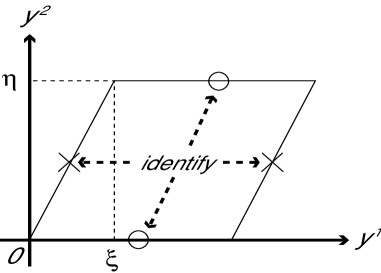
Figure 3: The shape of the torus is specified by $\xi$ and $\eta$. Both ends are understood to be identified.

The internal space we are considering is the direct product of the torus, $T_{2}\otimes T_{2}\otimes T_{2}$. Hence, the 10-dimensional metric to be consider is

$$ds^{2} = \bar{g}_{\mu\nu}dx^{\mu}dx^{\nu}+\sum_{a=1}^{3}\frac{b_{a}^{2}}{{\rm Im}\tau_{a}}\Big{|}dy^{2a-1}+\tau_{a}dy^{2a}\Big{|}^{2}\ ,$$ (52)

where we have defined three scale factor $b_{a}$ and the modulus $\tau_{a}$ for each torus with coordinates $y^{2a-1},y^{2a}$. We would like to analyze the stability of $T_{2}\otimes T_{2}\otimes T_{2}$ compacification. Fortunately, as the internal space is the direct product of torus, it is enough to investigate the simple 6-dimensional spacetime with one torus as the internal space.

Now, we shall take the metric

$$ds^{2} = \bar{g}_{\mu\nu}dx^{\mu}dx^{\nu}$$

$$\quad+\frac{b^{2}}{\eta}\left[(dy^{1}+\xi dy^{2})^{2}+\eta^{2}(dy^{2})^{2}\right]\ ,$$

where $\bar{g}_{\mu\nu}$ is the 4-dimensional metric in the Einstein frame and $b$ represents the scale factor of the torus, i.e. volume moduli. The anti-symmetric tensor field in 2-dimensions has only one component

$$B=\left(\begin{array}[]{cc}0&\beta\\ -\beta&0\end{array}\right)\ .$$ (56)

We call $\beta$ the flux moduli, hereafter. The 4-dimensional effective action in the Einstein frame becomes

$$S = \frac{V_{6}}{2\kappa^{2}}\int d^{4}x\sqrt{-\bar{g}}\left[\bar{R}-2(\partial\bar{\phi})^{2}-2(\partial\log b)^{2}\right.$$

$$\left.\quad-\frac{1}{2\eta^{2}}\left\{(\partial\eta)^{2}+(\partial\xi)^{2}\right\}-\frac{1}{2b^{4}}(\partial\beta)^{2}\right]$$

$$-\mu_{4}\int d^{4}x\sqrt{-\bar{g}_{00}}\sqrt{\bar{g}^{ij}p_{i}p_{j}+e^{2\bar{\phi}}M^{2}(\beta,b,\eta,\xi)}\ ,$$

where the mass is given by

$$M^{2}(\beta,b,\eta,\xi) = \frac{1}{\eta b^{2}}\left\{p_{1}\xi-p_{2}-\beta(w^{2}\xi+w^{1})\right\}^{2}$$ (58)

$$+\frac{\eta}{b^{2}}(p_{1}-w^{2}\beta)^{2}+\frac{b^{2}}{\eta}(w^{2}\xi+w^{1})^{2}$$

$$+\eta b^{2}(w^{2})^{2}+4(N-1)$$

$$-2(p_{1}w^{1}+p_{2}w^{2})\ .$$

Using Eq. (56) and

$$\Gamma = \frac{b^{2}}{\eta}\left(\begin{array}[]{cc}1&\xi\\ \xi&\ \xi^{2}+\eta^{2}\end{array}\right)$$ (61)

which one can read off from the metric (V). We see the above action has the T-duality symmetry (13) and (14) :

$$\tilde{\eta}=\frac{\eta}{\eta^{2}+\xi^{2}}\ ,\quad\tilde{\xi}=-\frac{\xi}{\eta^{2}+\xi^{2}}$$

$$\tilde{b}^{2}=\frac{b^{2}}{b^{4}+\beta^{2}}\ ,\quad\tilde{\beta}=-\frac{\beta}{b^{4}+\beta^{2}}\ .$$ (62)

From Eq. (62), it is easy to find the self-dual point

$$b=1\ ,\quad\eta=1\ ,\quad\xi=0\ ,\quad\beta=0\ .$$ (63)

One may expect this self-dual point is a stable minimum of the effective potential. In order to verify this, we should examine where is the minimum of $M^{2}(\beta,b,\eta,\xi)$ in the potential in the action (V). First, let us consider the string gas consisting of modes $N=1,p_{1}=w^{1}=1,p_{2}=w^{2}=0$ which becomes massless at the self-dual point. For this gas, we have

$$M^{2}_{1}=\frac{1}{\eta b^{2}}(\xi-\beta)^{2}+\frac{\eta}{b^{2}}+\frac{b^{2}}{\eta}-2$$ (64)

In this case, there exists flat directions $b^{2}=\eta\ ,\xi=\beta$ in contrast to the naive expectation. However, we only considered one kind of string gas which winds around one specific cycle. Apparently, we have the other cycle for the torus. Hence, we consider another string gas consisting of modes $N=1,p_{1}=w^{1}=0,p_{2}=w^{2}=1$ which becomes massless at the self-dual point. In this case, we obtain

$$M^{2}_{2}=\frac{1}{\eta b^{2}}(1+\beta\xi)^{2}+\frac{\eta\beta^{2}}{b^{2}}+\frac{b^{2}\xi^{2}}{\eta}+\eta b^{2}-2\ .$$ (65)

Now, we also have flat directions $\beta^{2}=\frac{b^{4}\xi^{2}}{\eta^{2}}\ ,1+\beta\xi=\eta b^{2}$. We find these two flat directions intersect at the self-dual point $b=1\ ,\eta=1\ ,\xi=0,\beta=0$. Hence, by taking into account both type of string gas, the self-dual point would be stable minimum. The stability can be explicitly verified by expanding the potential around this extrema as

$$V=\mu_{4}\sqrt{\frac{\bar{g}^{ij}p_{i}p_{j}}{g_{s}}}+\frac{1}{2}\frac{\mu_{4}e^{2\bar{\phi}}}{\sqrt{\bar{g}^{ij}p_{i}p_{j}}}M^{2}(\beta,b,\eta,\xi)$$ (66)

where we have used the fact that $M^{2}\approx 0$ near the self-dual point. Let us linearize the scale factor $b$ and the modulus $\eta$ as $b=1+\delta b$ and $\eta=1+\delta\eta$. Other variables $\xi$ and $\beta$ are already linear because the background values of these variables are zero. Hence, we have

$$\delta M^{2}_{1}=(\xi-\beta)^{2}+(\delta\eta-2\delta b)^{2}$$ (67)

and

$$\delta M^{2}_{2}=(\xi+\beta)^{2}+(\delta\eta+2\delta b)^{2}\ .$$ (68)

Here, we can see each potential has flat directions. However, by adding up both contributions, we get

$$\delta M^{2}=\delta M^{2}_{1}+\delta M^{2}_{2}=2\xi^{2}+2\beta^{2}+2\delta\eta^{2}+8\delta b^{2}$$ (69)

where flat directions disappear. Thus, we have proved the stability of all of the moduli of the torus. Even if we add other massless modes, the result does not change. The dilaton is also stabilized due to the reason explained in the previous section. This concludes the stability of $T_{2}\otimes T_{2}\otimes T_{2}$ compacification as we expected.

VI Conclusion

We have analyzed the stability of $T_{2}\otimes T_{2}\otimes T_{2}$ compactification in the context of massless string gas cosmology. We emphasized the importance of the T-duality and massless modes in a string. We have first performed the numerical calculations and then shown the stability of the dilaton. To understand this numerical result we have constructed the 4-dimensional effective action by taking into account the T-duality. It turned out that the dilaton is marginally stable. We performed the stability analysis of the volume moduli, the shape moduli and the flux moduli. We have found that all of these moduli are stabilized at the self dual point in the moduli space.

Of course, what we have shown is the stability of moduli during the string gas dominated stage. After the string gas dominated stage, the ordinally matter come to dominate the universe. Then, the dilaton will start to run. Therefore, we need to find a mechanism to stabilize the dilaton in these periods. One possibility is the non-perturbative string correction

$$S = \frac{1}{2\kappa^{2}}\int d^{10}x\sqrt{-G}\left[B_{1}(\phi)R+4B_{2}(\phi)(\partial\phi)^{2}\right.$$ (70)

$$\left.\qquad\qquad-\frac{1}{12}B_{3}(\phi)H^{2}\right]\ ,$$

where we have taken into accounts the loop corrections

$$B_{i}(\phi)=e^{-2\phi}+c_{i}e^{2\phi}+d_{i}e^{4\phi}+\cdots\ .$$ (71)

There may be a possibility to stabilize all of the moduli in the whole history of the universe in this context Damour:1994ya ; Damour:1994zq . This possibility deserve further investigations. It is also interesting to investigate the possibility to combine the string gas approach with other ones Kachru ; Berndsen:2005qq .

More importantly, we need a mechanism to explain the present large scale structure of the universe in the context of the string gas scenario. In the string gas model, it is difficult to realize the inflationary scenario. We might have to seek a completely different one from the inflationary generation mechanism of primordial fluctuations Battefeld:2005wv .