The 6D SuperSwirl

Abstract:

We present a novel supersymmetric solution to a nonlinear sigma model coupled to supergravity. The solution represents a static, supersymmetric, codimension-two object, which is different to the familiar cosmic strings. In particular, we consider 6D chiral gauged supergravity, whose spectrum contains a number of hypermultiplets. The scalar components of the hypermultiplet are charged under a gauge field, and supersymmetry implies that they experience a simple paraboloid-like (or 2D infinite well) potential, which is minimised when they vanish. Unlike conventional vortices, the energy density of our configuration is not localized to a string-like core. The solutions have two timelike singularities in the internal manifold, which provide the necessary boundary conditions to ensure that the scalars do not lie at the minimum of their potential. The 4D spacetime is flat, and the solution is a continuous deformation of the so-called “rugby ball” solution, which has been studied in the context of the cosmological constant problem. It represents an unexpected class of supersymmetric solutions to the 6D theory, which have gravity, gauge fluxes and hyperscalars all active in the background.

1 Introduction

Sigma models in quantum field theory constitute one of the most interesting theories with a wide range of applications in high energy physics. One of the most remarkable examples of this is represented in the linear sigma model theories, by the (non)-abelian Higgs model, where a complex scalar field has a Mexican hat potential. This theory has interesting static solitonic solutions, which are the well known vortices (for a review, see e. g. [1]). When coupled to gravity, these solitons give rise to codimension-two objects, or cosmic strings, which have the effect of producing a conical singularity in spacetime, and which could have been formed in early stages of the universe’s evolution, with important implications for cosmology [2]. Recently, cosmic strings with a superstring origin have also been considered due to its relevance for possible connections between string theories and experiment [3]. In this context, cosmic string solutions, or vortex solutions to (non)-abelian Higgs models coupled to supergravity, have been considered recently, with interesting results [4]. Other global and local supersymmetric codimension-two solutions to abelian Higgs models have been considered in a different context in three dimensions [5, 6]. Moreover, string-like solutions in nonlinear sigma models (i.e. those with non-canonical kinetic terms) have long been known to exist [7].

In this note, we would like to consider a particular nonlinear sigma model, which is coupled to gauged 6D supergravity [8], and study new examples of static, codimension-two, supersymmetric configurations, different from cosmic strings. Nonlinear sigma models appear quite generically in this context, because once scalar fields (which can arise in matter or supergravity multiplets) are coupled to supergravity, they always seem to form such structures [9]. This allows an elegant geometrical treatment of what would otherwise seem a highly intractable nonlinear system. Moreover, gauged supergravities are coming to the fore in recent years, since they describe the low energy effective theory of string theory compactifications with fluxes. There, the sigma model describes the moduli of the compactification, and the fluxes gauge certain isometries of the sigma model manifold, inducing a scalar potential in the theory. Indeed, in contrast to bosonic sigma models, where there is no unique way to construct a gauge invariant potential, for supersymmetric theories, supersymmetry (SUSY) is often powerful enough to determine the form of the potential uniquely. In general, it will be different to the familiar Mexican hat shape.

In this paper, we concentrate our attention on six dimensional chiral gauged supergravity [10, 11, 12, 13], in which a complex scalar field, $\phi$, has a paraboloid-like potential with a minimum at $\phi=0$ [14]. We are interested in static configurations which represent codimension-two objects in space-time and, moreover, preserve some fraction of the supersymmetry of the original system.

The model under consideration

The 6D supergravity theory that we study here has received much attention in the past, mainly due to its interesting phenomenological applications. For example, it shares many of the features of 10D supergravity — and so also of string vacua — such as the existence of chiral fermions [10] with nontrivial Green-Schwarz anomaly cancellation [15], as well as the possibility of having chiral compactifications down to flat four dimensions [10].

In its minimal form, the bosonic spectrum contains the graviton, dilaton, and antisymmetric two- and three-form field strengths. The gauging of a global R-symmetry, together with supersymmetry, requires the presence of a positive definite potential for the dilaton, with a Liouville form.

The presence of anomalies can be avoided by adding to the spectrum a number of hypermultiplets, suitably charged under the gauge group [10], rendering the theory consistent also at the quantum level. The scalars of the hypermultiplets appear in the potential, which has a minimum only when they vanish.

By switching on a magnetic monopole, the field equations admit a background solution of the form $R^{4}\times S^{2}$, that preserves half of the supersymmetries of the vacuum, and stabilises one of the moduli in the spectrum. This configuration was discovered by Salam and Sezgin (SS) [16]. It represents one of the simplest examples of flux compactification down to four dimensions, in which partial moduli stabilisation is achieved [17].

Moreover, it has been recently shown [18], that under certain assumptions, an important property of this theory is that the SS flux compactification is unique. More precisely, the authors of [18] showed that - for the minimal theory - if one limits one’s attention to vacua of the form $M_{4}\times M_{2}$, where $M_{4}$ is a four dimensional space-time with maximal symmetry, and $M_{2}$ a compact, regular two dimensional manifold, then the theory admits a unique supersymmetric configuration: the Salam-Sezgin one.

Thanks to the relative simplicity of the theory, it is interesting to ask whether, by renouncing the assumptions of [18], other potentially interesting supersymmetric compactifications exist. For example, by considering different space-time factorisations, the authors of [19] determined solutions of the form $AdS_{3}\times S^{3}$, as well as dyonic string configurations; generalisations of the latter have been found in [14].

Interestingly, new classes of supersymmetric solutions can alternatively be found by renouncing the hypothesis of regularity of the internal manifold. The simplest example is the rugby ball vacuum, which is obtained by slicing a wedge from the sphere, and which allows in this way the presence of conical singularities at the poles. This vacuum provides a setting for the supersymmetric large extra dimensions (SLED) brane world scenario of [20]. Here, the conical singularities are interpreted as codimension-two brane worlds, where the Standard Model fields can be localized. The model has been introduced as a possible way to tackle the cosmological constant problem [21] (for a non SUSY version, see [22]). More generally, this construction shows how singular supersymmetric configurations can nevertheless be interesting as settings for brane world models, in which supersymmetry may help to ensure the stability of the bulk geometry, at least at the classical level.

Our results

By renouncing the hypothesis of regularity, we show that further supersymmetric vacua do exist, preserving four dimensional maximal symmetry (they are 4D flat). They are obtained by turning on the hyperscalars contained in the hypermultiplets, which are necessary for anomaly cancellation. In this way, we have all kinds of fields in the theory active - gravity, gauge fields and scalars - which are consistent with the symmetries of the problem. The hyperscalar action corresponds to a nonlinear sigma model defined on a non-compact, quaternionic manifold. The scalar fields are coupled to gravity and to gauge fields, and have a potential with a global minimum at zero . The study of sigma models in six dimensions, coupled only to gravity, has been performed in [23, 24], both in the supersymmetric and non-supersymmetric case. However, as far as we are aware, our solutions constitute the first supersymmetric configurations in the full 6D gauged supergravity, in which the potential for the hyperscalar fields, required by supersymmetry, is included. Given our field content, we are able to find the most general supersymmetric solution, which has maximal 4D symmetry and axial symmetry in the internal 2D space.

Interestingly, the possibility to find a supersymmetric solution with the hyperscalars turned on is naively not expected for this theory. Indeed, the potential has a global minimum at the origin. Nevertheless, we show that a solution can be found, which preserves half of the supersymmetries of the vacuum. Similar to conventional vortices, the hyperscalars generate a configuration with a nonzero winding around the 2D manifold. As usual, this winding is induced by the coupling to the gauge field, as we will discuss. However, there are also significant differences to the smooth vortex solutions that are generated by a Higgs potential and spontaneous symmetry breaking. In particular, vortices have a well-defined core, at the center of which the scalar field sits at the top of its potential, where its amplitude is zero, $\phi=0$. Far away from the core, the scalar takes its minimum energy value. Especially for vortices generated by a local symmetry breaking, the energy density of the vortex is localized near to the core. In contrast, in our solutions the energy density is not confined to a string-like region, and the scalar field is nowhere vanishing, which here means that it does not reach the minimum of its potential. Moreover, the smooth central core that arises in vortices, is replaced by two singularities, which pinch off the internal manifold making its volume finite.

The singularities and winding are both needed for our configuration, since otherwise the hyperscalars would lie at the minimum of their potential, where they vanish. The resulting geometry is continuously connected to the rugby ball configuration, when the hyperscalars are set to zero. When the hyperscalars are switched on, the geometry deforms, but maintains nevertheless a ${\mathbb{Z}}_{2}$ reflection symmetry. The curvature singularities at the poles transform from conical to more serious ones, which are the sources for the hyperscalar fields. Given the novelty of this codimension-two supersymmetric configuration, we introduce a new name to define it; we call this new object the SuperSwirl.

Outline

The paper is organized as follows. Section (2) contains a technical, but necessary discussion of the explicit construction of the action for the 6D gauged supergravity. The hyperscalar part of the action, in particular, depends on the choice of the quaternionic manifold that the hyperscalars parameterise. The reader interested only in the final form of the sigma model that we consider, can jump this section and go directly to Section (3). In Section (3) we discuss in detail the 6D nonlinear sigma model that we are interested in. We analyse the conditions necessary to preserve some of the supersymmetry, taking a general ansatz for the fields involved. In Section (4) we derive the supersymmetric solution, and discuss its properties. In Section (5) we discuss the physical implications of this configuration, and we conclude.

2 The Six Dimensional Theory

2.1 Lagrangian, equations of motion, and susy transformations

We consider the six-dimensional ${\mathcal{N}}=(1,0)$ gauged supergravity constructed by Nishino-Sezgin (NS) in [13]. The particle content of this theory consists of various fields: a gravity multiplet $(e_{M}^{\it Q},\,\Psi_{M_{L}}^{A},\,B_{MN}^{-})$; a tensor multiplet $(B_{MN}^{+},\,\chi_{{}_{R}}^{A},\,\varphi)$; Yang-Mills multiplets $(A^{\hat{I}}_{M},\,\lambda_{{}_{L}}^{{\hat{I}}A})$; and the hypermatter multiplets $(\Psi^{a}_{{}_{R}},\,\Phi^{\alpha})$; where $A=1,2$, $a=1,\dots,2n$, $\alpha=1,\dots,4n$, with $n$ the number of hypermultiplets. Also, $M=(\mu\,,m)$ are spacetime indices in $d=6$ dimensions and ${\it Q}=(\hat{\mu}\,,q)$ are flat tangent indices. The gravitino, dilatino and gaugini are all $Sp(1)$ Majorana-Weyl spinors, and the hyperini are $Sp(n)$ Majorana-Weyl spinors.

The bosonic part of the corresponding Lagrangian is given by [13]

$$e^{-1}{\cal L}_{B} = \,\frac{1}{4}\,R-\frac{1}{4}\,\partial_{M}\varphi\,\partial^{M}\varphi-\frac{1}{2}\,G_{\alpha\beta}(\Phi)\,D_{M}\Phi^{\alpha}\,D^{M}\Phi^{\beta}$$ (2)

$$\qquad-\,\frac{1}{12}\,e^{2\varphi}\;G_{MNP}G^{MNP}-\,\frac{1}{4}\,e^{\varphi}\;F^{\hat{I}}_{MN}F_{\hat{I}}^{MN}-\,\frac{1}{8}\,e^{-\varphi}\,v(\Phi)\,.$$

Here as usual, $e=\sqrt{-det\,g}$, where $g_{MN}$ is the 6D spacetime metric. The Kalb-Ramond field strength is given by $G_{MNP}=(\partial_{M}B_{NP}+F^{\hat{I}}_{MN}A^{\hat{I}}_{P}-\frac{1}{3}g^{\prime}f^{ijk}A^{i}_{M}A^{j}_{N}A^{k}_{P}-\frac{1}{3}gf^{IJK}A^{I}_{M}A^{J}_{N}A^{K}_{P})+{\rm 2\,\,\,perms}$. The index $\hat{I}$ runs over the adjoint of $Sp(n)\times Sp(1)$, and so can be subdivided into the adjoint of $Sp(n)$: $\hat{I}=I=1,\dots,n(2n+1)$, and the adjoint of $Sp(1)$: $\hat{I}=i={\it 1,2,3}$. The structure constants of the gauge group are then labelled by $f^{IJK}$ and $f^{ijk}$. Supersymmetry requires that the hyperscalars parameterize a quaternionic manifold:

$$\frac{G}{H}=\frac{Sp(n,1)}{Sp(n)\times Sp(1)}\,,$$ (3)

whose metric is $G_{\alpha\beta}(\Phi)$. Thus the index $\alpha=1,\dots 4n$ can be interpreted as the curved index on this target space manifold.

The geometry of the target manifold can be described by the Maurer-Cartan form, which is constructed from the coset-representative, $L$:

$$L^{-1}\partial_{\alpha}L={\mathcal{W}}^{\hat{X}}_{\alpha}T^{\hat{X}}+V^{aA}_{\alpha}T_{aA}\,.$$ (4)

Here, $T^{\hat{X}}$ ($\hat{X}=x\,,X$) and $T_{aA}$ are the anti-hermitian generators of $Sp(n)\times Sp(1)$ and the coset, respectively. Then, ${\mathcal{W}}^{\hat{X}}_{\alpha}$ transforms as the spin-connection on the target manifold $G/H$, and $V^{aA}_{\alpha}$ is the vielbein, carrying the tangent space indices $a=1,\dots,2n$ and $A=1,2$, which run over the fundamental of $Sp(n)\subset H$ and $Sp(1)\subset H$ respectively. The scalar potential then takes the form

$$v=C^{x\hat{I}}C^{x\hat{I}}$$ (5)

with

$$C^{x\hat{I}}=\left\{\begin{array}[]{l}C^{xI}=g{\mathcal{W}}^{x}_{\alpha}\xi^{\alpha I}\\ C^{xi}=g^{\prime}({\mathcal{W}}^{x}_{\alpha}\xi^{\alpha i}-\delta^{xi})\end{array}\right.\,.$$ (6)

This prepotential $C^{x{\it\hat{I}}}$ can also be calculated directly from the coset representative [8, 25] as follows:

$$C^{x\hat{I}}=2\,g^{\prime}\,\left(L^{-1}{T}^{\hat{I}}L\right)_{AB}T^{x}_{AB}\,.$$ (7)

The Killing vectors of the scalar manifold are $\xi^{\alpha\hat{I}}(\Phi)=T^{\hat{I}\alpha}_{\beta}\Phi^{\beta}$ (the $T^{\hat{I}\alpha}_{\beta}$ are anti-hermitian generators for the groups $Sp(n)$ and $Sp(1)$ in $G$). Finally, the covariant derivative of the scalars is given by:

$$D_{M}\Phi^{\alpha}=\partial_{M}\Phi^{\alpha}-g^{\prime}A^{i}_{M}\xi^{\alpha i}-gA^{I}_{M}\xi^{\alpha I}$$ (8)

Here, $g^{\prime}$ is the gauge coupling of the $Sp(1)$ group, and $g$ that of the $Sp(n)$ group. The explicit definitions in terms of the scalars depends on the choice of coset representative, to be discussed in the next subsection.

The bosonic equations of motion derived from the corresponding action are:

$$\Box\,\varphi-\frac{1}{3}\,e^{2\varphi}\,G_{MNP}\,G^{MNP}-\frac{1}{2}\,e^{\varphi}\;F^{\hat{I}}_{MN}F^{MN}_{\hat{I}}+\frac{1}{4}\,e^{-\varphi}\,v(\Phi)=0$$

$$D_{M}\Bigl{(}e^{2\varphi}\,G^{MNP}\Bigr{)}=0$$ (9)

$$D_{M}\Bigl{(}e^{\varphi}\,F^{MN}_{\hat{I}}\Bigr{)}-e^{2\varphi}\,G^{MPN}\,F_{{\hat{I}}MP}+\hat{g}\,g^{MN}(D_{M}\Phi^{\alpha})\,\xi_{\alpha\hat{I}}=0$$

$$D^{M}D_{M}\Phi^{\alpha}+\Gamma^{\alpha}_{\beta\gamma}D^{M}\Phi^{\beta}D_{M}\Phi^{\gamma}-\frac{1}{8}G^{\alpha\beta}(\Phi)\,v_{\beta}(\Phi)\,e^{-\varphi}=0$$

$$R_{MN}-\partial_{M}\varphi\,\partial_{N}\varphi-2G_{\alpha\beta}(\Phi)\,D_{M}\Phi^{\alpha}\,D_{N}\Phi^{\beta}-e^{2\varphi}\,G_{MPQ}\,{G_{N}}^{PQ}$$

$$\qquad\qquad\qquad-2\,e^{\varphi}\,F_{MP}^{\hat{I}}{F_{{\hat{I}}N}}^{P}+\frac{1}{2}\,(\Box\varphi)\,g_{MN}=0,$$

where $v_{\beta}=\frac{\partial v}{\partial\Phi^{\beta}}$. Also, $\hat{g}=g\,{\rm or}\,g^{\prime}$ depending on the gauge sector. The supersymmetry transformation rules for the fermions are (up to fermion bi-linears):

$$\delta\chi^{A}=-\frac{1}{2}\partial_{M}\varphi\Gamma^{M}\epsilon^{A}+\frac{1}{12}e^{\varphi}G_{MNL}\Gamma^{MNL}\epsilon^{A}$$ (10)

$$\delta\Psi^{A}_{M}=D_{M}\epsilon^{A}+\frac{1}{24}e^{\varphi}G_{NLR}\Gamma^{NLR}\Gamma_{M}\epsilon^{A}$$ (11)

$$\delta\lambda^{A\hat{I}}=\frac{1}{2\sqrt{2}}e^{\varphi/2}F_{MN}^{\hat{I}}\Gamma^{MN}\epsilon^{A}-\frac{1}{\sqrt{2}}e^{-\varphi/2}C^{x\hat{I}}T^{xA}_{B}\epsilon^{B}$$ (12)

$$\delta\Psi^{a}=(D_{M}\Phi^{\alpha})\,V^{aA}_{\alpha}\Gamma^{M}\epsilon_{A}\,.$$ (13)

Recall that all spinors are symplectic-Majorana Weyl. The gravitini, Killing spinor, gaugini, and dilatini are all in the fundamental of $Sp(1)\subset H$, whereas the hyperini are in the fundamental of $Sp(n)\subset H$. The $T^{xA}_{B}$ are the generators of $Sp(1)\subset H$. The gaugini are also in the adjoint of $Sp(n)\times Sp(1)\subset G$.

The covariant derivative acting on the Killing spinor is given by:

$$D_{M}\epsilon^{A}=\partial_{M}\epsilon^{A}+\frac{1}{4}\omega_{M}^{\it PQ}\Gamma_{\it PQ}\epsilon^{A}+g^{\prime}A_{M}^{i}\delta^{ix}T^{xA}_{B}\epsilon^{B}+(D_{M}\Phi^{\alpha}){\mathcal{W}}_{\alpha}^{x}T^{xA}_{B}\epsilon^{B}$$ (14)

where, as before, ${\it P,\,Q}$ are flat tangent indices on the spacetime manifold. Note also that the last term, involving a coupling with the scalars, is due to the fact that the Killing spinor behaves as a section on the $Sp(1)$-bundle of the target manifold.

2.2 Parameterization of the Target Manifold

We can express the scalars $\Phi^{\alpha}$ ($\alpha=1,\dots,4n$), as an $n$-component quaternionic vector, $t^{p}$ ($p=1,\dots,n$). So, for example, $t^{p=1}=\Phi_{1}1+\Phi_{2}\hat{\i}+\Phi_{3}j+\Phi_{4}k$, where we use the following $2\times 2$ basis of quaternions:

$$\hat{\i} = \left(\begin{array}[]{cc}-i&\,\,0\\ \,\,0&\,\,i\end{array}\right)\,=\,-i\sigma_{3}\qquad\qquad j=\left(\begin{array}[]{cc}0&-1\\ 1&\,\,0\end{array}\right)\,=\,-i\sigma_{2}$$ (19)

$$k = \left(\begin{array}[]{cc}\,\,0&-i\\ -i&\,\,0\end{array}\right)\,=\,-i\sigma_{1}\qquad\qquad 1=\left(\begin{array}[]{cc}\,\,1&\,\,0\\ \,\,0&\,\,1\end{array}\right)$$ (24)

We need to choose a specific parameterization of the target manifold, in order to have explicit expressions for the metric, $G_{\alpha\beta}(\Phi)$, and potential, $v(\Phi)$, which appear in the field equations. A choice of coset representative, $L$ – where $L$ is an $Sp(n,1)$ valued matrix – is sufficient to define all necessary quantities. Following [13], we choose this matrix to be:

$$L=\gamma^{-1}\left(\begin{array}[]{cc}1&t^{\dagger}\\ t&\Lambda(t)\end{array}\right)$$ (25)

where

$$\gamma=(1-t^{\dagger}t)^{1/2}\,,\phantom{000000}\Lambda(t)=\gamma(I-tt^{\dagger})^{-1/2}$$ (26)

Here, $I$ is the $n\times n$ unit matrix, and ^† refers to matrix transposition and quaternionic conjugation ($a+b\hat{\i}+cj+dk\rightarrow a-b\hat{\i}-cj-dk$). The Maurer-Cartan form $(L^{-1}\partial_{\alpha}L)$ can now be decomposed as:

$$L^{-1}\partial_{\alpha}L=\left(\begin{array}[]{cc}{\mathcal{W}}_{\alpha}^{AB}&V_{\alpha}^{\dagger Ab}\\ V_{\alpha}^{aB}&{\mathcal{W}}_{\alpha}^{ab}\end{array}\right)$$ (27)

where ${\mathcal{W}}_{\alpha}^{AB}={\mathcal{W}}_{\alpha}^{x}T^{x\,AB}$ and ${\mathcal{W}}_{\alpha}^{ab}={\mathcal{W}}_{\alpha}^{X}T^{X\,ab}$ are the $Sp(1)$ and $Sp(n)$ connections, and $V_{\alpha}^{aB}$ is the pullback of the vielbein. From these expressions it follows that:

$${\mathcal{W}}_{\alpha}^{AB} = \frac{1}{2}\gamma^{-2}\left(\partial_{\alpha}t^{\dagger}\,t-t^{\dagger}\partial_{\alpha}t\right)$$ (28)

$${\mathcal{W}}_{\alpha}^{ab} = \gamma^{-2}\left(-t\partial_{\alpha}t^{\dagger}+\Lambda\partial_{\alpha}\Lambda+\frac{1}{2}\partial_{\alpha}(t^{\dagger}t)I\right)$$

$$V_{\alpha}^{aA} = \gamma^{-1}\left(I-tt^{\dagger}\right)^{-1/2}\partial_{\alpha}t$$

Choosing to turn on only two “real” components of the full quaternion ($\Phi_{1}$, $\Phi_{3}$), and using the above relations, the relevant metric components can be calculated from:

$$G_{\alpha\beta}=V_{\alpha}^{aA}\epsilon_{ab}\epsilon_{AB}V_{\beta}^{bB}$$ (29)

and are given by:

$$G_{11} = V_{1}^{aA}V_{1aA}=\frac{2}{(1-\Phi_{1}^{2}-\Phi_{3}^{2})^{2}}$$ (30)

$$G_{33} = V_{3}^{aA}V_{3aA}=\frac{2}{(1-\Phi_{1}^{2}-\Phi_{3}^{2})^{2}}$$ (31)

$$G_{13} = V_{1}^{aA}V_{3aA}=0$$ (32)

Here, we have used that the flat indices are raised and lowered with the metric $\epsilon_{AB}=\epsilon^{AB}=[(0,1),(-1,0)]$ and $\epsilon_{ab}$. Also, we split the indices $a=1,\dots,2n$ into $a=pA^{\prime}$, with $p=1\dots n$ and $A^{\prime}=1,2$, and use $\epsilon_{ab}={\sf 1}_{pq}\otimes\epsilon_{A^{\prime}B^{\prime}}$.

In order to calculate the potential, we use an explicit form for the Killing vectors. For simplicity, we will take the $Sp(n)$ gauge coupling to zero in what follows, that is, $g=0$. Moreover, we consider only the gauging of the $U(1)$ subgroup, that is, from now on we take $i={\it 1}$. The Killing vectors are then:

$$\xi^{{\it 1}\alpha} = T^{{\it 1}\alpha}_{\beta}\Phi^{\beta}$$ (33)

$$= T^{{\it 1}\alpha}_{1}\Phi_{1}+T^{{\it 1}\alpha}_{3}\Phi_{3}$$

We choose the conventions for the relevant generator, $T^{{\it 1}\,\alpha}_{\beta}$: $T^{{\it 1}\alpha}_{\beta}=T^{{\it 1}A}_{B}\otimes{\sf 1}^{a}_{b}$, with $T^{{\it 1}A}_{B}=1/2\,([0,-1],[1,0])$, $A=1,3$. Now, we can compute the $C$ function from the definition in (6), using the explicit values for ${\mathcal{W}}_{\alpha}^{x}$, obtained from (28) in terms of the two non zero fields, $(\Phi_{1},\,\Phi_{3})$. We find:

$$C^{x{\it 1}}=-\frac{g^{\prime}}{1-\Phi_{1}^{2}-\Phi_{3}^{2}}\qquad\qquad{\rm for}\qquad x={\it 1},$$

$$\hskip 22.76228pt=0\hskip 113.81102pt{\rm otherwise}$$ (34)

The potential is then

$$v=C^{x{\it 1}}C^{x{\it 1}}=\frac{g^{\prime 2}}{(1-\Phi_{1}^{2}-\Phi_{3}^{2})^{2}}\,.$$ (35)

We have found in this way all the quantities that characterize our nonlinear sigma model. Using the above relations, we can now write explicit expressions for the action, equations of motion and supersymmetry transformations in terms of a single complex scalar field defined as

$$\phi=\Phi_{1}+i\Phi_{3}\,,\qquad\qquad\phi^{\star}=\Phi_{1}-i\Phi_{3}\,,$$ (36)

We do this in the next section.

3 The Model

The bosonic action for our 6D nonlinear sigma model (2), in terms of (36), reduces to

$$e^{-1}{\cal L}_{B}=\,\frac{1}{4}\,R-\frac{1}{4}\,\partial_{M}\varphi\,\partial^{M}\varphi-\frac{1}{(1-|\phi|^{2})^{2}}\,D_{M}\phi\,D^{M}\phi^{\star}-\,\frac{1}{4}\,e^{\varphi}\;F_{MN}F^{MN}-\,\frac{1}{8}\,\frac{g^{\prime 2}\,e^{-\varphi}}{(1-|\phi|^{2})^{2}}\,\,,$$

The equations of motion for our system then become:

$$\Box\,\varphi=\frac{1}{2}\,e^{\varphi}\;F_{MN}F^{MN}-\frac{g^{\prime 2}}{4}\,\frac{e^{-\varphi}}{(1-|\phi|^{2})^{2}}\,,$$

$$D_{M}\Bigl{(}e^{\varphi}\,F^{MN}\Bigr{)}=\frac{ig^{\prime}}{2(1-|\phi|^{2})^{2}}\,g^{MN}(\phi^{\star}D_{M}\phi-\phi D_{M}\phi^{\star})\,,$$

$$R_{MN}=\partial_{M}\varphi\,\partial_{N}\varphi+\frac{2}{(1-|\phi|^{2})^{2}}(D_{M}\phi D_{N}\phi^{\star}+D_{M}\phi^{\star}D_{N}\phi)$$

$$\hskip 142.26378pt+\,2e^{\varphi}\,F_{MP}F_{N}^{\,\,\,P}-\frac{1}{2}\,(\Box\varphi)\,g_{MN}\,,$$

$$D^{M}D_{M}\phi+\frac{2\phi^{\star}}{(1-|\phi|^{2})}D^{M}\phi D_{M}\phi=\,\frac{g^{\prime 2}e^{-\varphi}}{4}\frac{\phi}{(1-|\phi|^{2})}\,.$$ (38)

Here we also have to add an equation for the complex conjugate of the scalar field. In terms of the complex field, the scalar manifold metric is:

$$d\sigma^{2}=2\frac{d\phi d\phi^{\star}}{(1-|\phi|^{2})^{2}}\,.$$ (39)

The covariant derivatives are given by:

$$D_{M}\phi=\partial_{M}\phi-\frac{ig^{\prime}}{2}A_{M}\phi\,,$$ (40)

$$D^{M}D_{M}\phi=\nabla^{M}D_{M}\phi-\frac{ig^{\prime}}{2}A^{M}\,D_{M}\phi\,,$$ (41)

where $\nabla_{M}$ is the covariant derivative with respect to the metric:

$$\nabla^{M}D_{M}\phi=\frac{1}{\sqrt{g}}\partial_{M}(\sqrt{g}\,g^{MN}\,D_{N}\,\phi)\,,$$

and equivalently for the complex conjugate field $\phi^{\star}$.

The supersymmetry transformations (10-13) can be written as:

$$\delta\chi=-\frac{1}{2}\partial_{M}\varphi\Gamma^{M}\,\epsilon$$ (42)

$$\delta\Psi_{M}=D_{M}\epsilon$$ (43)

$$\delta\lambda=\frac{e^{\varphi/2}}{2\sqrt{2}}F_{MN}\Gamma^{MN}\,\epsilon+\frac{i}{\sqrt{2}}\frac{g^{\prime}\,e^{-\varphi/2}}{(1-|\phi|^{2})}\,\epsilon$$ (44)

$$\delta\Psi=\frac{1}{2\,(1-|\phi|^{2})}D_{M}\phi\,\Gamma^{M}\,\epsilon\,.$$ (45)

Here, all spinors are complex-Weyl and we have defined them as $\epsilon=\epsilon_{1}+i\epsilon_{2}$.

3.1 Supersymmetry conditions

We consider the most general ansatz consistent with 4D maximal symmetry. Thus, we take:

$$ds^{2}=e^{2W(z,\bar{z})}\,g_{\mu\nu}\,dx^{\mu}dx^{\nu}+e^{2B(z,\bar{z})}dzd\bar{z}\,,$$

$$F^{\hat{I}}_{MN}=F_{mn}(z,\bar{z})\,,\qquad\varphi=\varphi(z,\bar{z})\,,\qquad\phi=\phi(z,\bar{z})\,.$$ (46)

where $g_{\mu\nu}$ is the 4D metric on de Sitter, Minkowski or anti-de Sitter spacetime, and $z,\,\bar{z}$ are complex coordinates in the internal 2 dimensions. All other fields are zero.

We now look at the supersymmetry transformations, to find what conditions must be satisfied by the fields in order to ensure that the system preserves some fraction of the total supersymmetry. Since all the fermion fields vanish, we need only concern ourselves with the transformation laws of the fermions.

$\delta\chi=0$: Plugging our ansatz above into the SUSY transformations, we see immediately from the dilatino condition that the dilaton must be constant:

$$\varphi=\varphi_{0}\,=\,{\rm constant}\,.$$ (47)

$\delta\lambda=0$: From the gaugino condition, we have:

$$\frac{1}{2}F_{MN}\Gamma^{MN}\,\epsilon=-i\frac{g^{\prime}\,e^{-\varphi_{0}}}{(1-|\phi|^{2})}\,\epsilon\,.$$ (48)

Writing $F_{q\bar{q}}=if(z,\bar{z})\varepsilon_{q\bar{q}}$, with $f=f^{\star}$, and where $q,\,\bar{q}$ are the internal, flat, complexified indices and $\varepsilon_{q\bar{q}}=\varepsilon^{q\bar{q}}=1$, gives us:

$$f(z,\bar{z})\Gamma_{\bar{q}q}\,\epsilon=-\frac{g^{\prime}\,e^{-\varphi_{0}}}{2}\frac{1}{(1-|\phi|^{2})}\,\epsilon\,.$$ (49)

In order to satisfy this condition, we impose the following projections on the spinors

$$\Gamma_{\bar{q}q}\,\epsilon=\epsilon\,,\qquad\qquad\Gamma_{\bar{q}q}\,\epsilon^{\star}=-\epsilon^{\star}$$ (50)

which imply the following condition between the flux and the potential

$$f=-\frac{g^{\prime}}{2}\frac{e^{-\varphi_{0}}}{(1-|\phi|^{2})}$$ (51)

The projection condition (50), breaks one half of the 6D supersymmetries, thus leaving ${\mathcal{N}}=1$ from a four dimensional point of view.

$\delta\Psi=0$: The SUSY condition for the hyperino, gives us immediately

$$D_{\bar{z}}\,\phi\,\epsilon=0\,,\qquad\qquad D_{z}\,\phi^{\star}\,\epsilon^{\star}=0\,,$$ (52)

where $D_{\bar{z}}\phi=\partial_{\bar{z}}\phi-i\,\frac{g^{\prime}}{2}A_{\bar{z}}\phi$. Because we require non-vanishing spinors, this implies that the complex scalar field must be covariantly holomorphic, that is

$$D_{\bar{z}}\,\phi\,=\,0\,,\qquad\qquad D_{z}\,\phi^{\star}\,=\,0\,$$ (53)

$\delta\psi_{M}=0$: The last SUSY transformation is that for the gravitino. In order to compute this, we need the values of the space-time spin connection. For example, when the non-compact directions are Minkowski $g_{\mu\nu}=\eta_{\mu\nu}$, the nonzero components are given by:

$$\omega^{\hat{\mu}q}_{\,\,\,\,\,\,\mu}=\sqrt{2}\,e^{W-B}W_{\bar{z}}\,\delta^{\hat{\mu}}_{\,\,\mu}\,,\qquad\omega^{\hat{\mu}\bar{q}}_{\,\,\,\,\,\,\mu}=\sqrt{2}\,e^{W-B}W_{z}\,\delta^{\hat{\mu}}_{\,\,\mu}\,,$$

$$\omega^{\bar{q}q}_{\,\,\,\,\,\,z}=-B_{z}\,,\qquad\qquad\qquad\,\,\,\,\omega^{\bar{q}q}_{\,\,\,\,\,\,\bar{z}}=B_{\bar{z}}\,,$$ (54)

where $\hat{\mu}$ and $q(\bar{q})$ are flat indices. Assuming that the spinor $\epsilon$ is a function only of $z,\,\bar{z}$, from the $M=\mu$ component of the gravitino equation;

$$\omega^{\,\,\,{\it PQ}}_{\mu}\,\Gamma_{\it PQ}\,\epsilon=0\,,$$ (55)

we can see that, for a 4D Minkowski solution,

$$W(z,\bar{z})\,=\,{\rm constant}\,.$$

On the other hand, for de Sitter or anti-de Sitter 4D spacetimes, the condition (55) imposes additional projection conditions on the Killing spinor, which break the remaining ${\cal N}=1$ supersymmetry in 4D. For example, for the AdS metric in Poincaré coordinates: $ds^{2}=e^{2W}\left(l^{2}/v^{2}\right)\left(-dt^{2}+dv^{2}+dx^{2}+dy^{2}\right)+e^{2B}dzd\bar{z}$, we again arrive at $W(z,\bar{z})\,=\,{\rm constant}$, but furthermore find that we must impose:

$$\Gamma_{\hat{\mu}\hat{v}}\epsilon=0$$ (56)

These projections break a further half of the original supersymmetries. In order to avoid this situation, which would leave us with less than one supersymmetry at the four dimensional level, we are forced to consider a flat 4D spacetime.

Now considering the $M=m=z,\bar{z}$ components of the gravitino transformation, we find:

$$\partial_{m}\epsilon+\frac{1}{2}\omega_{m}^{\,\,\bar{q}q}\Gamma_{\bar{q}q}\,\epsilon+\frac{ig^{\prime}A_{m}}{2}\,\epsilon+\frac{1}{2\,\left(1-|\phi|^{2}\right)}\Big{[}\phi D_{m}\phi^{\star}-\phi^{\star}D_{m}\phi\Big{]}\,\epsilon=0\,,$$ (57)

and its complex conjugate. One can see from these equations that

$$\epsilon\,\epsilon^{\star}=constant\,.$$ (58)

Equation (57) for $\epsilon$ is the last equation that must be satisfied in order to preserve supersymmetry. To ensure that such a Killing spinor exists locally, it is sufficient to impose the following integrability condition:

$$0\,=\,\left[D_{z},D_{\bar{z}}\right]\,\epsilon^{A}\,=\,\left(B_{z\bar{z}}+\frac{D_{z}\phi D_{\bar{z}}\phi^{\star}}{\left(1-|\phi|^{2}\right)^{2}}+\frac{1}{2}e^{2B+\varphi_{0}}\,f^{2}\right)\epsilon^{A}\,,$$ (59)

where in the last equality we have applied the conditions that emerge from the preceding transformations. We must now check whether the above constraints are consistent with the equations of motion.

3.2 The equations of motion

The supersymmetry constraints allow us to obtain and satisfy the equations of motion. Indeed, the equation for the dilaton, $\varphi$, requires:

$$\frac{1}{2}F_{MN}F^{MN}=\frac{g^{\prime 2}}{4}\frac{e^{-2\varphi_{0}}}{(1-|\phi|^{2})^{2}}\,.$$ (60)

Plugging the value of $F_{mn}$ into the equation above gives us

$$f^{2}=\frac{g^{\prime 2}}{4}\frac{e^{-2\varphi_{0}}}{(1-|\phi|^{2})^{2}}\,,$$ (61)

which is precisely (51). The equation of motion for $\varphi$ is consequently satisfied.

The equation of motion for the gauge field is:

$$\frac{1}{\sqrt{g}}\partial_{M}(\sqrt{g}\,e^{\varphi_{0}}F^{MN})=\frac{ig^{\prime}}{2(1-|\phi|^{2})^{2}}\,g^{MN}(\phi^{\star}D_{M}\phi-\phi D_{M}\phi^{\star})\,.$$ (62)

Taking into account that $F^{z\bar{z}}=-2ife^{-2B}$, $\sqrt{g}=e^{2B}/2$, and using (53), we obtain

$$if_{z}=\frac{g^{\prime}\,e^{-\varphi_{0}}}{2i\left(1-|\phi|^{2}\right)^{2}}\left[\phi^{\star}D_{z}\phi\right]\,,$$ (63)

and its complex conjugate. Using the supersymmetry condition (53) on this equation we find

$$f_{z}=-\frac{g^{\prime}\,e^{-\varphi_{0}}}{2}\frac{1}{(1-|\phi|^{2})^{2}}[\phi^{\star}\phi_{z}+\phi\phi^{\star}_{z}]\,.$$ (64)

which is just the derivative of (51).

It is straightforward to check that the Einstein equations for the components ($\mu\nu$), $(z,z)$ and ($\bar{z},\bar{z}$) are automatically satisfied for covariantly holomorphic scalar fields, constant dilaton and no warping. On the other hand, the relation between the gauge function $f$ and the hyperscalars (51), together with the antiholomorphicity condition, implies that the hyperscalar equation of motion is also satisfied.

Finally, the ($z,\,\bar{z}$) component of the Einstein’s equations gives us

$$\frac{1}{2}\,B_{z\bar{z}}=-\frac{D_{z}\phi D_{\bar{z}}\phi^{\star}}{2\left(1-|\phi|^{2}\right)^{2}}-\frac{1}{4}e^{2B+\varphi_{0}}\,f^{2}\,.$$ (65)

This equation coincides with the integrability constraint (59), so once this equation is satisfied, it ensures that supersymmetry is preserved. The equation provides a constraint on the function $B$ that must be satisfied in order to obtain a solution. So we have seen that all the field equations can be obtained from the supersymmetry constraints.

We conclude this section by noticing that the supersymmetry constraints (51) and (53) are analogous to the Landau-Ginzburg equations that describe linear sigma-model vortices in a supergravity setting [4, 5, 6]. In our system, we are able to solve exactly the resulting equations of motion. The important difference with the usual case is in the form of the potential, which, in our case, is required by supersymmetry to have a minimum at the origin. For this reason, the solutions that we will find have similarities but also significant differences to the usual vortex solutions.

4 The SuperSwirl

4.1 Determining the solution

In the last section we obtained the constraints that the geometry and Killing spinors must satisfy in order to have a supersymmetric configuration. We find that all the equations of motion are automatically satisfied, once we impose the supersymmetry constraints and we are left with only one nontrivial equation coming from the $(z,\bar{z})$ component of the Einstein equation:

$$\frac{1}{2}\,B_{z\bar{z}}=-\frac{D_{z}\phi D_{\bar{z}}\phi^{\star}}{2\left(1-|\phi|^{2}\right)^{2}}-\frac{1}{4}e^{2B+\varphi_{0}}\,f^{2}\,,$$ (66)

while eq. (53) and its complex conjugate are:

$$\partial_{\bar{z}}\,\phi=\frac{ig^{\prime}}{2}\,A_{\bar{z}}\,\phi\,,\qquad\qquad\qquad\partial_{z}\,\phi^{\star}=-\frac{ig^{\prime}}{2}\,A_{z}\,\phi^{\star}\,.$$ (67)

Defining

$$\phi=\psi^{\frac{1}{2}}\,e^{i\tau}\,,$$ (68)

the fields that we have to determine are $\tau$, $B$, and $\psi$. We start by extracting some information from (67). It is simple to show, starting from these formulae, that, whenever $\psi\neq 0$, the following equations hold

$$\partial_{z\bar{z}}\ln{\psi} = \frac{ig^{\prime}}{2}\,(\partial_{z}A_{\bar{z}}-\partial_{\bar{z}}A_{z})\,=\,\frac{ig^{\prime}}{2}F_{z\bar{z}}$$ (69)

$$\partial_{z\bar{z}}\,\tau = \frac{g^{\prime}}{4}\,(\partial_{z}A_{\bar{z}}+\partial_{\bar{z}}A_{z})$$ (70)

Notice that the following gauge transformation leaves invariant these two equations:

$$A_{z}\,\to A_{z}+\partial_{z}T\,,$$ (71)

$$\phi\,\to e^{ig^{\prime}\,T/2}\phi\,.$$ (72)

In terms of the fields $\psi$ and $\tau$ the gauge transformation is

$$\psi\,\to\psi\,,$$ (73)

$$\tau\,\to\tau+\frac{g^{\prime}}{2}\,T\,.$$ (74)

Determining B

Remembering that

$$f=-\frac{g^{\prime}}{2}\frac{e^{-\varphi_{0}}}{(1-|\phi|^{2})}\,\left(=\,-2iF_{z\bar{z}}\,e^{-2B}\right)\,,$$ (75)

eq. (66) can be rewritten as

$$B_{z\bar{z}}=-\frac{\partial_{z\bar{z}}\ln{\psi}}{(1-\psi)}-\frac{\partial_{z}\psi\,\partial_{\bar{z}}\psi}{\psi\,(1-\psi)^{2}}=\partial_{z\bar{z}}[\ln{(\psi^{-1}-1)}]\,.$$ (76)

Thus we can integrate this equation, to obtain:

$$e^{B}\,=\frac{\left(1-\psi\right)}{\psi}\,F^{1/2}(z)F^{\star 1/2}(\bar{z})\,.$$ (77)

In this way, we have found a direct relation between $\psi$ and the metric function $B$, given in (77). Alternatively, a relation between these two quantities is obtained comparing eq. (75) and eq. (69). One finds

$$e^{2B}=\frac{8\,e^{\varphi_{0}}}{g^{\prime 2}}\,(1-\psi)\,\partial_{z\bar{z}}\ln{\psi}\,.$$ (78)

Determining $\psi$

Comparing (77) and (78) one obtains the following differential equation for $\psi$, which must be solved to obtain a SUSY solution:

$$\frac{8\,e^{\varphi_{0}}}{g^{\prime 2}}\,\partial_{z\bar{z}}\ln{\psi}\,=\,\frac{\left(1-\psi\right)}{\psi^{2}}\,F(z)F^{\star}(\bar{z})\,.$$ (79)

If regular enough, the function $F$ can be re-absorbed into the two dimensional metric by a rescaling of the coordinate $z$:

$$dz\,\to\,F(z)\,dz\,.$$

For this reason we can set it equal to an arbitrary real integration constant, $\tilde{c}$, without loss of generality. Thus we can rewrite (79) as

$$\partial_{z\bar{z}}\ln{\psi}\,=\,c\,\frac{\left(1-\psi\right)}{\psi^{2}}\,,$$ (80)

where the constant $c$ is given by

$$c=\frac{g^{\prime 2}\,e^{-\varphi_{0}}\,\tilde{c}^{2}}{8}\,.$$ (81)

The most general supersymmetric solution with the matter content that we are considering, preserving 4D maximal symmetry, corresponds to the most general solution to the modified Liouville equation given in (80).

Determining $\epsilon$

We can now integrate the Killing spinor equation (57) explicitly. Using (50, 53, 3.1) and (77) as discussed above, this equation gives the solution:

$$\epsilon(z,\bar{z})=e^{i\tau(z,\bar{z})}\,\epsilon_{0}$$ (82)

where $\epsilon_{0}$ is a constant spinor. This solution indeed satisfies (58).

The solution

An exact solution to equation (80) can be obtained by asking that $\psi$ depends on some real combination of $(z,\bar{z})$, for example by 

$$x\equiv z+\bar{z}\,.$$

In this case, it is simple to show that (80) can be reduced to a first order differential equation

$$\left(\frac{d}{dx}\ln{\psi}\right)^{2}\,=\,c\left(\frac{2\psi-1}{\psi^{2}}\right)+\alpha^{2}\,,$$ (83)

where $\alpha^{2}$ is a positive real constant . Eq. (83) can be reassembled in the following way

$$\alpha^{2}\left(\psi+\frac{c}{\alpha^{2}}\right)^{2}-\left(\frac{d}{dx}\psi\right)^{2}\,=\,\left(c+\frac{c^{2}}{\alpha^{2}}\right)$$ (84)

At this point, it is easy to show that the general solution for the equation (84) is given by

$$\psi=\frac{1}{e^{\alpha x}}\,\left[M+N\,e^{\alpha x}+P\,e^{2\alpha x}\right]\,,$$ (85)

where the real numbers $M$, $N$, $P$ are integration constants  that satisfy the condition

$$N=-\frac{c}{\alpha^{2}}=\frac{1}{2}\left(1-\sqrt{1+16MP}\right)\,.$$ (86)

Since $\psi$ is real and positive, this implies that $M,\,P\geq 0$.

4.2 Properties of the SuperSwirl

4.2.1 Axial symmetry

The general supersymmetric solution above, eq. (85), can be seen to constitute the most general axially symmetry solution that preserves supersymmetry, and maximal space-time symmetry in 4D. This becomes evident after performing the following change of coordinates

$$e^{2z}\,=\,re^{i\theta}\,\qquad,\qquad e^{2\bar{z}}\,=\,re^{-i\theta}\,.$$

that allows one to identify the variable $x$ of the previous section with $\ln{r}$. The general solution depending on the variable $x$, determined in the previous section, in these coordinates depends only on the radial coordinate $r$, and, consequently, it is axially symmetric.

More explicitly, a simple calculation shows that in terms of these new coordinates, the solution  now reads (a ^′ means derivative along $r$)

$$ds_{6}^{2} = \eta_{\mu\nu}\,dx^{\mu}dx^{\nu}+e^{2B(r)}\left(dr^{2}+r^{2}d\theta^{2}\right)\,,$$ (87)

$$\phi = \psi^{\frac{1}{2}}e^{i\,g^{\prime}\,T/2}\,,$$ (88)

$$\varphi = \varphi_{0}\,,$$ (89)

$$F_{r\theta} = -\frac{g^{\prime}\,e^{-\varphi_{0}}\,\tilde{c}^{2}}{8}\frac{(1-\psi)}{r\,\psi^{2}}\,,$$ (90)

$$A_{\theta} = -\frac{r}{g^{\prime}}\frac{\psi^{\prime}}{\psi}+\partial_{\theta}T\,.$$ (91)

with the definitions and constraints (notice that we have redefined the function $B$ as the conformal factor for the internal metric in polar coordinates; $e^{2B}dzd\bar{z}\rightarrow e^{2B}(dr^{2}+r^{2}d\theta^{2})$):

$$e^{2B} = \frac{\tilde{c}^{2}}{4}\,\frac{(1-\psi)^{2}}{r^{2}\,\psi^{2}}\,,$$ (92)

$$\psi = \frac{1}{r^{\alpha}}\,\left(M-\frac{c}{\alpha^{2}}\,r^{\alpha}+P\,r^{2\alpha}\right)\,,$$ (93)

$$c = \frac{g^{\prime 2}\,e^{-\varphi_{0}}\,\tilde{c}^{2}}{8}=\,\frac{\alpha^{2}}{2}\left(\sqrt{1+16MP}-1\right).$$ (94)

4.2.2 Singularity structure

The singularity structure can be read from the metric function $e^{2B}$ given in formula (110). When the hyperscalars are turned on, the solution has unavoidable (see Appendix), timelike singularities (the scalar invariants diverge) at the points at which this function vanishes, or diverges. This occurs at the positive zeros of the function $1-\psi=0$, where the conformal factor $e^{2B}$ vanishes. These are located at

$$r_{\pm}^{\alpha}\, = \,\frac{1}{2P}\,\sqrt{\frac{1+\sqrt{1+16MP}}{2}}\,\left(\sqrt{\frac{1+\sqrt{1+16MP}}{2}}\pm 1\right)$$ (95)

$$= \,\frac{1}{2P}\,\sqrt{1+\frac{c}{\alpha^{2}}}\,\left(\sqrt{1+\frac{c}{\alpha^{2}}}\pm 1\right)\,.$$ (96)

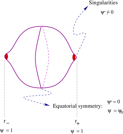
Figure 1: Pictorial representation of the internal two dimensional geometry of the superswirl. The two points at the ends of the space are singular. These are located at the positions where $\psi=1$. The first derivative – or speed – of the scalar field, does not vanish $\psi_{\pm}^{\prime}\neq 0$ at these points. There is an equatorial symmetry at the position $r_{0}$, where the scalar field’s first derivative vanishes $\psi_{0}^{\prime}=0$. This picture can also be understood from the point of view of the potential, in an interesting way, see fig. (2).

The presence of these singularities is perhaps not surprising, since the 6D potential and target-space metric, blow up at these positions. The physical space-time lies in the coordinate range $r_{-}\leq r\leq r_{+}$. Let us now show how the singularities arise in this spacetime. Consider for example the limit $r\to r_{-}$. The relevant part of the metric is

$$ds_{2}^{2}\,=\,e^{2B(r)}\,\left(dr^{2}+r^{2}\,d\theta^{2}\right)\,,$$ (97)

with $e^{2B}$ given in eq. (110). Performing the coordinate transformation

$$r^{\alpha}\,=\,\sqrt{\rho}\,\sqrt{\frac{4}{\tilde{c}}\,\frac{\alpha\,r_{-}^{\alpha}}{\left(r_{+}^{\alpha}-r_{-}^{\alpha}\right)}}\,+\,r_{-}^{\alpha}\,,$$ (98)

brings the metric (97), for $\rho\to 0$ (that is, $r\to r_{-}$), to the form

$$ds_{2}^{2}\,\sim\,d\rho^{2}+\gamma\,\rho\,d\theta^{2}\,,$$ (99)

with $\gamma=4\,\tilde{c}\,\alpha\,r_{-}^{\alpha}(r_{-}^{\alpha}-r_{+}^{\alpha})$. This implies that near $r_{-}$ the metric does not have a conical singularity, but a more serious one.

Notice that the space still closes off on approaching the singularity, in the sense that a circumference that surrounds the singularity reduces its radius when approaching it. The same is true for the limit $r\to r_{+}$. Moreover, a simple calculation shows that the internal manifold has a finite volume.

The singularities constitute sources for the hyperscalars. Indeed, the field $\psi$ and its first derivative do not vanish on approaching the end of the space at the singularities $r_{+}$, $r_{-}$: consequently, a source producing these fields, with the right boundary conditions, should be located at the position of the singularities.

4.2.3 Global constraints

One can see from the expressions for the solution in eq. (91) that the gauge field strength vanishes at the position of the singularities. This indicates that the sources are not coupled to the magnetic field. We therefore ask that the gauge potential also be vanishing at the singularities. The gauge field is given by

$$A_{\theta}(r)\,=\,-\frac{r}{g^{\prime}}\frac{\psi^{\prime}}{\psi}+a\,,$$ (100)

where $a$ is an integration constant corresponding to the gauge freedom, that is, choosing the function $T$ in (91) as

$$T\,=\,a\,\theta+2b/g^{\prime}\,,$$ (101)

with $a$ and $b$ real numbers.

In order to have a gauge field vanishing at both $r=r_{\pm}$, it must be defined locally over two overlapping patches, with two different integration constants:

$$a^{+}\,=\,\frac{r_{+}}{g^{\prime}}\,\psi^{\prime}(r_{+})\,;\qquad\quad a^{-}\,=\,\frac{r_{-}}{g^{\prime}}\,\psi^{\prime}(r_{-})\,.$$

Since the hyperscalars are charged under the gauge field (71), they must also be locally defined: $\phi^{\pm}=\psi^{1/2}(r)e^{i\tau^{\pm}}$, with $\tau^{\pm}=g^{\prime}a^{\pm}\,\theta/2+b$ . Since $\phi$ must be single-valued over the period $\theta=(0,2\pi)$, there is a constraint on the integration constants:

$$\frac{g^{\prime}}{2}\,a^{\pm}=n^{\pm}\,\,;\qquad\qquad n^{\pm}\in{\mathbb{Z}}\,.$$ (103)

Inserting the values for $a^{\pm}$ in (4.2.3) into this expression, we find a topological condition on the parameters of the solution:

$$\frac{\alpha}{2}\,\sqrt{1+\frac{c}{\alpha^{2}}}\,=\,n^{+}=-n^{-}\,.$$ (104)

We thus see that the total winding inside the internal space vanishes as it should. Moreover, we also require that $A^{\pm}(r)$ (and $\phi^{\pm}(r,\theta)$) are related in the overlap by a single-valued gauge transformation:

$$A^{+} = A^{-}+\partial_{\theta}\Lambda$$ (105)

$$\phi^{+} = \phi^{-}\,e^{i\frac{g^{\prime}}{2}\Lambda}\,,$$ (106)

which leads to a Dirac quantization condition. Given (103), we see that the conditions above are indeed satisfied:

$$a^{-}-a^{+}\,=\,\frac{2m}{g^{\prime}}\,,$$ (107)

where $m\in{\mathbb{Z}}$. From here we immediately find that $m=2n^{+}$.

The previous discussion indicates that the global constraints on the gauge fields generate a winding of the hyperscalars around the singularities. These fields, on each side of the equator are given by

$$\phi^{\pm}=\psi(r)^{1/2}\,e^{i(n^{\pm}\theta+b)}\,,$$ (108)

with $n^{\pm}$ integer numbers, and they smoothly join at the equator where $\psi^{\prime}$ vanishes.

We conclude this subsection returning to the issue of supersymmetry for our solution. Plugging the superswirl solution with the global constraints we have just discussed, into (82), we obtain the explicit solution for the Killing spinor, which is given by:

$$\epsilon\,=\,\epsilon_{0}\,e^{i(n^{\pm}\theta+b)}\,,$$ (109)

where $\epsilon_{0}$ is, again, a constant spinor. From this expression, we explicitly show that the Killing spinor for our configuration is single valued, since after an interval of $2\pi$ (the period of the $\theta$ coordinate) the spinor (109) returns to itself.

4.2.4 The rugby ball limit

We now show that in the limit when the hyperscalars go to zero in a proper way, we recover the rugby ball solution [16, 21]. Such a limit, $\psi\to 0$, is obtained by properly sending $M$, $c$ and $P$ to zero. The function $e^{2B}$ can be rewritten as

$$e^{2B}=\frac{2\,c\,e^{\varphi_{0}}}{MP\,g^{\prime 2}}\,\frac{1}{r^{2}}\,\frac{\left(r^{\alpha}-M+\frac{c}{\alpha^{2}}r^{\alpha}-Pr^{2\alpha}\right)^{2}}{\left[\left(\frac{M}{P}\right)^{\frac{1}{2}}-\frac{c}{\sqrt{MP}\,\alpha^{2}}r^{\alpha}+\left(\frac{P}{M}\right)^{\frac{1}{2}}r^{2\alpha}\right]^{2}}$$ (110)

From eq.(86) we learn that, when $M$ and $P\to 0$,

$$c\to 0\,\qquad\,,\,\qquad\,\frac{c}{\sqrt{MP}}\to 0\,\qquad\,,\,\qquad\,\frac{c}{MP}\to 4\alpha^{2}\,.$$ (111)

So eq. (110) becomes, if $M$ and $P\to 0$ at the same rate,

$$e^{2B}=\frac{8\,e^{\varphi_{0}}\,\alpha^{2}}{g^{\prime 2}}\,\frac{1}{r^{2}}\,\frac{1}{\left[\left(\frac{r}{r_{0}}\right)^{\alpha}+\left(\frac{r}{r_{0}}\right)^{-\alpha}\right]^{2}}\,,$$ (112)

with

$$r_{0}=\left(\frac{M}{P}\right)^{\frac{1}{2\alpha}}\,,$$ (113)

and this is nothing but the rugby ball in non-standard coordinates. In order to see this explicitly, one makes the change of coordinates:

$$\left(\frac{r}{r_{0}}\right)^{\alpha}=\tan{\frac{\chi}{2}}\,.$$ (114)

In these coordinates the two dimensional metric becomes:

$$ds^{2}=a_{0}^{2}(d\chi^{2}+\alpha^{2}\sin^{2}{\chi}\,d\theta^{2})$$ (115)

where $a_{0}^{2}=2e^{\varphi_{0}}/g^{\prime 2}$ is the radius of the 2-sphere and $\alpha$ is related to the deficit angle. One can similarly check that the gauge field also acquires the right monopole limit .

4.2.5 Equatorial symmetry

Although singular, our solution enjoys an equatorial symmetry similar to the rugby ball one: the solution has a reflection symmetry on a hypersurface that we can call the equator. For the rugby ball in the coordinates of eq. (112), it is simple to see that the equatorial symmetry is translated to the symmetry $r\to\frac{r_{0}^{2}}{r}$. The point $r_{0}$ is the position of the equator, and is a fixed point for the reflection symmetry. In our case exactly the same is true. It is indeed simple to show that both the scalar (93) and the metric (97) are invariant under the operation

$$r\,\to\,\frac{r_{0}^{2}}{r}\,,$$ (116)

with the same $r_{0}$ given in (113). We illustrate the global structure of the solution in Fig. (1).

4.2.6 Energy

We can now compute explicitly the energy per unit four dimensional volume of the superswirl. As expected, the energy turns out to diverge, due to the contributions from the boundaries. Indeed, the energy can be computed from (see e.g. [4])

$${\mathcal{E}} = \int{dr\,d\theta}\,\sqrt{g}\,\left[\frac{1}{4}R+\frac{D_{m}\phi\,D^{m}\phi^{\star}}{(1-|\phi|^{2})^{2}}+\frac{1}{4}e^{\varphi_{0}}F_{mn}F^{mn}+\frac{1}{8}\frac{g^{\prime 2}\,e^{-\varphi_{0}}}{(1-|\phi|^{2})^{2}}\right]$$ (117)

$$+\,\frac{1}{2}\left(\int{d\theta\,\sqrt{h}\,{\mathcal{K}}}|_{r=r_{+}}-\int{d\theta\,\sqrt{h}\,{\mathcal{K}}}|_{r=r_{-}}\right)\,,$$

where ${\mathcal{K}}$ is the extrinsic curvature of the surfaces $r=constant$, whose metric is $h$. In our case these surfaces are the “boundaries” at $r_{\pm}$. For our solution (87-90) this energy can be expressed in a Bogomol’nyi type form as follows:

$${\mathcal{E}} = \frac{1}{2}\int{dr\,d\theta\,\frac{1}{r}\left[\frac{\left|\,r\,D_{r}\phi+i\,D_{\theta}\phi\,\right|^{2}}{(1-|\phi|^{2})^{2}}+e^{\varphi_{0}}\left(f+\frac{g^{\prime}\,e^{\varphi_{0}}}{2\,(1-|\phi|^{2})}\right)^{2}\right]}$$ (118)

$$+\frac{1}{2}\left(\int{d\theta\,r\,B^{\prime}}|_{r_{+}}-\int{d\theta\,r\,B^{\prime}}|_{r_{-}}\right)\,.$$

Here we have used the ($z,\,\bar{z}$) component of Einstein’s equations (or the gravitino integrability constraint) to express $R$ in terms of the matter fields. From this expression is clear that the supersymmetry constraints (51) and (53) in terms of the $(r,\,\theta)$ coordinates, imply the vanishing of the first two terms of the energy. Thus the energy is given entirely by the last two terms. These are given by

$${\mathcal{E}}=-\pi\,\left(\frac{r\,\psi^{\prime}}{1-\psi}+\frac{r\,\psi^{\prime}}{\psi}\right)\Bigg{|}_{r_{+}}+\pi\,\left(\frac{r\,\psi^{\prime}}{1-\psi}+\frac{r\,\psi^{\prime}}{\psi}\right)\Bigg{|}_{r_{-}}\,.$$ (119)

Here we have used the explicit expression for the derivative of $B$ in terms of $\psi$. It is simple to see that, at the boundaries where the curvature singularities are located, this quantity diverges, since there $\psi=1$. This signals the necessity to include explicit source terms for the hyperscalars, placed at the boundaries. Their presence can contribute with new terms to the calculation of the energy, rendering it finite by compensating the infinite contributions.

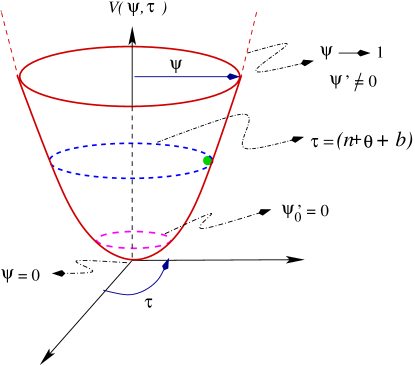
Figure 2: The structure of the superswirl solution in terms of the potential.

5 Discussion

We have determined and studied a static, supersymmetric, codimension-two configuration for a nonlinear sigma model, in the context of six dimensional gauged supergravity. For the matter content considered (whose bosonic part is a $U(1)$ gauge field, and a complex scalar field), it is the most general supersymmetric solution consistent with 4D maximal symmetry and axial symmetry in the internal space. The solution can be regarded as a deformation of the classical spherical compactification of Salam-Sezgin, due to a non trivial profile for the hyperscalars in the internal manifold. Although the internal manifold is non-compact, since the presence of hyperscalars produces singularities at the poles  of the geometry, it has a finite volume. The configuration is everywhere locally supersymmetric, except at the position of the singularities, $r_{\pm}$.

The presence of the singularities is an essential ingredient that allows the solution to exist: the singularities behave, indeed, as sources for the hyperscalar fields. Without these singularities, the complex hyperscalar field, by continuity, would need to vanish at the position of the poles of the compact manifold. This is because at the poles, the angular coordinate, along which the hyperscalar winds, is ill-defined. The presence of sources where the singularities are located, instead, allows for more general boundary conditions for the hyperscalars at the poles, and permits supersymmetry to be preserved away from the sources.

The exact supersymmetric solution that we have found has some similarities with the Landau-Ginzburg (LG) vortices studied in [5, 6] in 3 dimensions, as well as with the recent D-strings in 4 dimensions studied in [4]. Indeed, the conditions required to preserve some fraction of the supersymmetry, have the very same structure (see eqs. (51) and (53)). However, there are important differences between the LG vortices, the D-strings and our configuration. In the former cases, the sigma model considered is a linear one, and corresponds to the (non)-abelian Higgs model with a Mexican hat potential. This allows one to find smooth string solutions, with a well defined size for the core of the string, which depends on the inverse of the vacuum expectation value for the Higgs field. The scalar that generates the vortex vanishes by continuity at the origin, where the maximum of the potential is located, and asymptotically, it approaches the minimum of the potential outside the core of the vortex. The field has a winding around the symmetry axis, parameterized by an integer number $n$. This measures the tension of the string as seen from infinity, and represents a topological charge that ensures the stability of the system. Moreover, the tension of these strings is finite, as the boundary terms provide a finite contribution to it. Indeed, cosmic strings do not have any sources for the scalar fields, and thus, they are completely smooth and stable.

Our solution shares the property of the winding of the vortex. Here, the winding of the hyperscalars around the symmetry axis is parameterized by two integers $n^{\pm}$, which define the phase of the field, $\tau$. The integers $n^{\pm}$ are related to the Dirac quantization condition that the gauge potentials must satisfy, and they are equal and opposite. Thus, the total winding number vanishes, indicating a cancellation of the total charge inside the 2D internal space. This is also analogous to what happens in systems with vortex-anti-vortex pairs, in compact spaces.

Beyond the winding, however, the configuration constructed in this paper, has a somewhat different physical interpretation to conventional vortices. The underlying potential has a minimum at the origin, and has a paraboloid-like shape, diverging when $|\phi|=\psi^{\frac{1}{2}}=1$ (see figure (2)). The hyperscalar configuration that we determined, consequently does not have a core at the origin, but it is instead generated by the sources at the ends of the space, $r_{\pm}$, corresponding to the circle at $\psi=1$ where the potential diverges. It extends from $\psi=1$ to a value $\psi_{0}\equiv\psi(r_{0})<1$, which is characterized by the fact that $\psi^{\prime}(r_{0})=0$ ($\psi^{\prime}$ changes sign at $r_{0}$). In some sense, at that point the hyperscalar turns back and returns up the potential towards the source. The point $r_{0}$ corresponds, not surprisingly, to the position of the equator of the two dimensional internal manifold $M_{2}$. Indeed, we have shown that our system, with the hyperscalars included, is ${\mathbb{Z}}_{2}$ symmetric at the equator.

Finally, another important difference in our solution is the fact that the energy (per unit volume) is infinite, since it is proportional to the boundary terms computed at the singular points. This again indicates the fact that our system, contrary to the usual vortices, should have boundary source terms that cover the singularities. These should regularise the latter, rendering the total energy finite. For these reasons, our configuration, although similar in many aspects to the usual supersymmetric vortices/strings, possesses important differences. Given its novelty, we name it: the SuperSwirl.

This new solution constitutes a new class of supersymmetric vacua for 6D chiral gauged supergravity, with possible implications for a deeper understanding of the theory itself, in particular its origin from higher dimensional supergravities or string theories. A string realization of the Nishino-Sezgin (NS) gauged supergravity [13] has been found in [29]. Unfortunately, the hypermultiplet sector of the theory was not considered in their analysis. An alternative route for obtaining NS gauged supergravity is being developed in [30]. In any case, it would be nice to understand whether the superswirl has an interesting higher dimensional interpretation in terms of extended objects.

In the context of 6D brane world scenarios, the superswirl can provide a natural setting for a thick version of a codimension-two brane world, along the lines proposed in [26, 27, 28]. In this case, the singularities would be covered by a sort of thick three-brane. A possibility would be to place, at the position of the singularities or slightly before them, a four-brane on which the space ends, characterized by the fact that one of its spatial dimensions is compactified on a circle with small size. The fields living on the four-brane would be described by an action suitably coupled to the bulk fields, that can in principle be constructed along the lines of [31]. In terms of the SLED proposal for the cosmological constant problem, the superswirl is interesting since it provides another class of 4D flat solutions to which the system can evolve, and moreover the only other explicit supersymmetric solution known, apart from that of Salam-Sezgin. Bulk supersymmetry represents, naturally, a very important property of this model, since it contributes to maintaining the bulk stable. In general, we expect supersymmetry to nevertheless be broken at the position of the branes, as in the original codimension-two SLED proposal. It would be interesting to determine whether our model enables the construction of a brane action that preserves the bulk supersymmetry, for example along the lines of [32].

Appendix A Appendix

Let us show that it is not possible to find, in our system, regular configurations, with hyperscalars turned on, without sources for these fields. We proceed by contradiction. Consider eq. (77). This equation, remember, is obtained under the hypothesis that the $\psi$ field is not zero. The equation can be written as ($q$ is a positive constant)

$$\frac{q}{(1-\psi)}=e^{-2B}\partial_{z}\partial_{\bar{z}}\,\ln{\psi}$$ (120)

The right hand side of this equation can be written

$$e^{-2B}\partial_{z}\partial_{\bar{z}}\,\ln{\psi}=\nabla_{M}\nabla^{M}\,\ln{\psi}$$ (121)

where the indices $M$ run through $z$, $\bar{z}$.

Now, suppose that we find a solution for our system that describes a compact, everywhere regular manifold with no sources for the hyperscalar fields. This means that you can integrate both sides of (120) over the manifold. The RHS is zero, since, by (121), it is an integral of a total derivative over a regular, boundary-less space. The equation becomes

$$\int dzd\bar{z}\sqrt{g}\frac{q}{(1-\psi)}=0$$ (122)

Now, recalling that $\psi=|\phi|^{2}$ cannot be negative, equation (77) shows that the quantity $(1-\psi)$ must be positive, or at most null, everywhere.

Now, let us return to the integral (122). Since $\sqrt{g}=e^{2B}$ is also everywhere positive, the argument of the integral must be positive. So the integral cannot be equal to zero, as required. Therefore, the initial hypothesis that we can find a compact manifold everywhere regular leads us to a contradiction.

References

- [1] Topological solitons, N. Manton and P. Sutcliffe, Cambridge University Press, 2004.
- [2] Cosmic strings and other topological defects, A. Vilenkin, E. P. S. Shellard, Cambridge University Press, 1994.
- [3] See J. Polchinski, “Introduction to cosmic F- and D-strings,” arXiv:hep-th/0412244 and references therein.
- [4] G. Dvali, R. Kallosh and A. Van Proeyen, “D-term strings,” JHEP 0401, 035 (2004) [arXiv:hep-th/0312005]; J. J. Blanco-Pillado, G. Dvali and M. Redi, “Cosmic D-strings as axionic D-term strings,” arXiv:hep-th/0505172.
- [5] K. Becker, M. Becker and A. Strominger, “Three-dimensional supergravity and the cosmological constant,” Phys. Rev. D 51 (1995) 6603 [arXiv:hep-th/9502107].
- [6] J. D. Edelstein, C. Nunez and F. A. Schaposnik, “Supergravity and a Bogomolny bound in three-dimensions,” Nucl. Phys. B 458, 165 (1996) [arXiv:hep-th/9506147].
- [7] See e. g. G. W. Gibbons, M. E. Ortiz and F. R. Ruiz, “Existence Of Global Strings Coupled To Gravity,” Phys. Rev. D 39 (1989) 1546.
- [8] R. Percacci and E. Sezgin, “Properties of gauged sigma models,” arXiv:hep-th/9810183.
- [9] “Supergravities In Diverse Dimensions”, Vol. 1, 2. By A. Salam, (Ed.), E. Sezgin, (Ed.) (ICTP, Trieste), 1989. Amsterdam, Netherlands: North-Holland (1989) 1499 p. Singapore, Singapore: World Scientific (1989) 1499 p.
- [10] S. Randjbar-Daemi, A. Salam, E. Sezgin and J. A. Strathdee, “An Anomaly Free Model In Six-Dimensions,” Phys. Lett. B 151 (1985) 351.
-
[11]
S. D. Avramis, A. Kehagias and S. Randjbar-Daemi,
“A new anomaly-free gauged supergravity in six dimensions,”
JHEP 0505 (2005) 057
[arXiv:hep-th/0504033];
S. D. Avramis and A. Kehagias, “A systematic search for anomaly-free supergravities in six dimensions,” arXiv:hep-th/0508172. - [12] N. Marcus and J. H. Schwarz, “Field Theories That Have No Manifestly Lorentz Invariant Formulation,” Phys. Lett. B 115 (1982) 111.
- [13] H. Nishino and E. Sezgin, “Matter And Gauge Couplings Of N=2 Supergravity In Six-Dimensions,” Phys. Lett. B 144 (1984) 187; “The Complete N=2, D = 6 Supergravity With Matter And Yang-Mills Couplings,” Nucl. Phys. B 278 (1986) 353; “New couplings of six-dimensional supergravity,” Nucl. Phys. B 505 (1997) 497 [arXiv:hep-th/9703075].
- [14] S. Randjbar-Daemi and E. Sezgin, “Scalar potential and dyonic strings in 6d gauged supergravity,” Nucl. Phys. B 692 (2004) 346 [arXiv:hep-th/0402217].
-
[15]
M.B. Green, J.H. Schwarz and P.C. West,
“Anomaly Free Chiral Theories In Six-Dimensions,”
Nucl. Phys. B 254 (1985) 327;
J. Erler, “Anomaly cancellation in six-dimensions,” J. Math. Phys. 35 (1994) 1819 [hep-th/9304104]. - [16] A. Salam and E. Sezgin, “Chiral Compactification On Minkowski X S**2 Of N=2 Einstein-Maxwell Supergravity In Six-Dimensions,” Phys. Lett. B 147, 47 (1984).
- [17] Y. Aghababaie, C. P. Burgess, S. L. Parameswaran and F. Quevedo, “SUSY breaking and moduli stabilisation from fluxes in gauged 6D supergravity,” JHEP 0303 (2003) 032 [arXiv:hep-th/0212091].
- [18] G. W. Gibbons, R. Guven and C. N. Pope, “3-branes and uniqueness of the Salam-Sezgin vacuum,” Phys. Lett. B 595, 498 (2004) [arXiv:hep-th/0307238].
- [19] R. Guven, J. T. Liu, C. N. Pope and E. Sezgin, “Fine tuning and six-dimensional gauged N = (1,0) supergravity vacua,” Class. Quant. Grav. 21 (2004) 1001 [arXiv:hep-th/0306201].
- [20] For a review with many references see: C. P. Burgess, “Towards a natural theory of dark energy: Supersymmetric large extra dimensions,” AIP Conf. Proc. 743 (2005) 417 [arXiv:hep-th/0411140].
- [21] Y. Aghababaie, C. P. Burgess, S. L. Parameswaran and F. Quevedo, “Towards a naturally small cosmological constant from branes in 6D supergravity,” Nucl. Phys. B 680 (2004) 389 [arXiv:hep-th/0304256].
-
[22]
S. M. Carroll and M. M. Guica, “Sidestepping the
cosmological constant with football-shaped extra dimensions,”
[hep-th/0302067];
I. Navarro, “Codimension two compactifications and the cosmological constant problem,” JCAP 0309 (2003) 004 [hep-th/0302129];
I. Navarro, “Spheres, deficit angles and the cosmological constant,” Class. Quant. Grav. 20 (2003) 3603 [hep-th/0305014];
H. P. Nilles, A. Papazoglou and G. Tasinato, “Selftuning and its footprints,” Nucl. Phys. B 677 (2004) 405 [hep-th/0309042];
H. M. Lee, “A comment on the self-tuning of cosmological constant with deficit angle on a sphere,” Phys. Lett. B 587 (2004) 117 [arXiv:hep-th/0309050];
J. Vinet and J. M. Cline, “Can codimension-two branes solve the cosmological constant problem?” [hep-th/0406141];
M. L. Graesser, J. E. Kile and P. Wang, “Gravitational perturbations of a six dimensional self-tuning model,” [hep-th/0403074];
J. Vinet and J. M. Cline, “Codimension-two branes in six-dimensional supergravity and the cosmological constant problem,” Phys. Rev. D 71 (2005) 064011 [arXiv:hep-th/0501098]. - [23] V. P. Nair and S. Randjbar-Daemi, “Nonsingular 4d-flat branes in six-dimensional supergravities,” JHEP 0503 (2005) 049 [arXiv:hep-th/0408063].
-
[24]
A. Kehagias,
“A conical tear drop as a vacuum-energy drain for the solution of the
cosmological constant problem,”
Phys. Lett. B 600 (2004) 133
[arXiv:hep-th/0406025];
S. Randjbar-Daemi and V. A. Rubakov, “4d-flat compactifications with brane vorticities,” JHEP 0410 (2004) 054 [arXiv:hep-th/0407176];
H. M. Lee and A. Papazoglou, “Brane solutions of a spherical sigma model in six dimensions,” Nucl. Phys. B 705 (2005) 152 [arXiv:hep-th/0407208]. - [25] For the interested reader, we note here that we can convert from the conventions of [8] to those of [13], by making the replacement: . Notice then that the group action on the coset representative : , which in [8] for infinitessimal transformations is , , becomes in [13] , . This is why, in [13], the minimal couplings in the covariant derivatives of the scalars and fermions appear with opposite signs, even though we take the generators and with the same sign. Finally, notice that the covariant derivatives for the fermions in [8] are written , whereas in [13] they are: .
- [26] C. P. Burgess, F. Quevedo, G. Tasinato and I. Zavala, “General axisymmetric solutions and self-tuning in 6D chiral gauged supergravity,” JHEP 0411 (2004) 069 [arXiv:hep-th/0408109].
- [27] I. Navarro and J. Santiago, “Gravity on codimension 2 brane worlds,” JHEP 0502 (2005) 007 [arXiv:hep-th/0411250].
- [28] E. Papantonopoulos and A. Papazoglou, “Brane-bulk matter relation for a purely conical codimension-2 brane world,” arXiv:hep-th/0501112.
- [29] M. Cvetic, G. W. Gibbons and C. N. Pope, “A string and M-theory origin for the Salam-Sezgin model,” Nucl. Phys. B 677 (2004) 164 [arXiv:hep-th/0308026].
- [30] C. P. Burgess, S. L. Parameswaran and F. Quevedo, to appear.
- [31] Y. Aghababaie et al., “Warped brane worlds in six dimensional supergravity,” JHEP 0309 (2003) 037 [arXiv:hep-th/0308064].
- [32] E. Bergshoeff, R. Kallosh and A. Van Proeyen, “Supersymmetry in singular spaces,” JHEP 0010 (2000) 033 [arXiv:hep-th/0007044].