hep-th/0509011

Instabilities of Near-Extremal Smeared Branes

and the Correlated Stability Conjecture

Troels Harmark, Vasilis Niarchos, Niels A. Obers

The Niels Bohr Institute

Blegdamsvej 17, 2100 Copenhagen Ø, Denmark

harmark@nbi.dk, niarchos@nbi.dk, obers@nbi.dk

Abstract

We consider the classical and local thermodynamic stability of non- and near-extremal D$p$-branes smeared on a transverse direction. These two types of stability are connected through the correlated stability conjecture for which we give a proof in this specific class of branes. The proof is analogous to that of Reall for unsmeared branes, and includes the construction of an appropriate two-parameter off-shell family of smeared D$p$-brane backgrounds. We use the boost/U-duality map from neutral black strings to smeared black branes to explicitly demonstrate that non-and near-extremal smeared branes are classically unstable, confirming the validity of the conjecture. For near-extremal smeared branes in particular, we show that a natural definition of the grand canonical ensemble exists in which these branes are thermodynamically unstable, in accord with the conjecture. Moreover, we examine the connection between the unstable Gregory-Laflamme mode of charged branes and the marginal modes of extremal branes. Some features of T-duality and implications for the finite temperature dual gauge theories are also discussed.

1 Introduction

The gauge/gravity correspondence [1] implies a deep connection between the thermodynamics of near-horizon brane backgrounds and that of the dual non-gravitational theories. In particular, this suggests that the gauge theory dual of a classically unstable brane background must have a corresponding phase transition. This hints at an interesting connection between the classical stability of brane backgrounds and the thermodynamic stability of the dual non-gravitational theories, and thereby to the thermodynamic stability of the brane backgrounds themselves.

Gregory and Laflamme [2, 3] were the first to study the classical stability of neutral black strings, as well as certain charged branes. They showed that neutral black strings are unstable under perturbations that oscillate in the direction in which the string extends, provided that the wavelength of the perturbation is larger than the order of the horizon radius. When the extended direction is compactified on a circle, this means in particular that for masses below/above a critical mass the black string is unstable/stable. Already in this original work, a global thermodynamic argument for the instability was given, namely that for small masses the entropy of a localized black hole is higher than that of the black string with the same mass, suggesting a possible endpoint for the decay of the black string in that case.

This deep connection between classical and thermodynamic stability of brane solutions was recently made more precise with a conjecture formulated by Gubser and Mitra [7, 8]. The conjecture, referred to as the Correlated Stability Conjecture (CSC), states that for systems with translational symmetry and infinite extent, a Gregory-Laflamme (GL) instability arises precisely when the system has a local thermodynamic instability. In further detail, local thermodynamic stability is defined here as positive-definiteness of the Hessian matrix of second derivatives of the mass with respect to the entropy and any charges that can be redistributed over the direction in which the GL instability is supposed to occur. Thus, the CSC relates a local thermodynamic instability to a perturbative dynamical instability. The latter is the classical gravitational instability arising from perturbations of the brane background.

For magnetically charged D$p$-brane solutions in String/M-theory, a semi-classical proof of the CSC was given by Reall [9] using the Euclidean path integral formulation of gravity. A key ingredient in this proof is the relation between the threshold mode of the classical instability and a Euclidean negative mode in the semi-classical path integral. In this way, for this class of branes it was shown that a classical instability appears precisely when the specific heat becomes negative. The CSC has also been considered and confirmed recently in more complicated settings involving bound states of branes [15, 16, 17]. A class of counter-examples in a different setting appeared very recently in [18]. Further comments related to these examples can be found in Section 3.

Another interesting class of branes is that of smeared D$p$-branes. Here, we call an electrically charged brane smeared if it has a direction with translational symmetry along which the brane is not charged. For magnetically charged branes we follow the opposite convention. When compactified on the isometric direction, a smeared D$p$-brane is related by T-duality to a D$(p+1)$-brane wrapping the T-dual circle. In particular, the near-extremal limit of the latter has a dual description in terms of a $(p+1)$-dimensional supersymmetric Yang-Mills (SYM) theory compactified on a circle. Thus, the issue of stability of smeared black branes has non-trivial implications for the stability of the dual SYM theories on $\mathbb{R}^{p-2}\times\mathbb{T}^{2}$, where the torus consists of the compact spatial world volume direction and the Euclidean time direction.

Moreover, there is an interesting connection between neutral black strings and smeared D$p$-branes. Building on the original observation of Ref. [19], it was shown in [20] (see also [21, 22, 23]) that the phases of Kaluza-Klein black holes (see the reviews [5, 6, 24]) can be mapped onto phases of non- and near-extremal D$p$-branes with a circle in their transverse space. The map is a sequence of boost and U-duality transformations, and includes as a special case the map of neutral black strings to non- and near-extremal D$p$-branes that are uniformly smeared on a transverse circle.

For neutral black strings wrapped on a circle a new static phase of non-uniform strings [25, 26, 27, 28] is known to emerge at the GL transition point, where the unstable mode is at threshold. In Refs. [21, 22, 20] it was observed that the GL point is mapped onto a critical mass/energy for non-/near-extremal branes, where a new phase of non- and near-extremal branes, non-uniformly distributed on the circle, emerges. This picture strongly suggests that non- and near-extremal smeared branes exhibit classical instabilities. In particular, the threshold mode of the black string is mapped directly onto the threshold mode of non- and near-extremal smeared black D$p$-branes. More generally, it is natural to expect that the (time-dependent) unstable mode can also be obtained from the neutral GL unstable mode by a suitable generalization of the boost/U-duality map [22].

The aim of this paper is to study the classical stability and CSC for non- and near-extremal smeared branes in detail. Our analysis will show in a quantitative way how the presence of charge affects the GL instability of neutral black strings, and what happens when we take the near-extremal limit. An important tool that we use is the boost/U-duality map mentioned above. In this work we restrict ourselves to smeared D$p$-branes of type II string theory, but the other 1/2-BPS branes can be treated similarly.

The main points of this paper can be summarized as follows:

• We argue that when applying the CSC to smeared branes one should consider thermodynamic stability in the grand canonical ensemble since the charge can redistribute itself in the direction in which the brane is smeared. Non-extremal smeared branes are thermodynamically unstable in this ensemble and according to the CSC these branes should have a classical instability. The choice of ensemble is independent of whether the brane is electrically or magnetically charged.

• We give a proof of the CSC for smeared branes. One of the essential elements is the explicit construction of an appropriate off-shell two-parameter family of Euclidean backgrounds connected to these branes.

• Following Ref. [22], we give an explicit construction of the GL unstable mode for non-extremal smeared branes. More specifically, we map the time-dependent unstable GL mode of neutral black strings to a time-dependent unstable mode of non-extremal smeared branes. This confirms the validity of the CSC for non-extremal smeared branes.

• We present a detailed analysis of the near-extremal limit and the validity of the CSC in this case. We show explicitly that the near-extremal limit of the unstable GL mode of non-extremal smeared branes is well-defined and hence that near-extremal smeared branes are classically unstable. According to the CSC this means that near-extremal smeared branes are thermodynamically unstable in the grand canonical ensemble. Nevertheless, it seems that in the near-extremal limit the charge cannot vary anymore, and it is not a priori obvious how to define a grand canonical ensemble for these branes. We show, however, that a natural definition of such an ensemble exists. This implies a new version of the first law of thermodynamics for near-extremal smeared branes, involving a rescaled chemical potential. In this near-extremal grand canonical ensemble, the near-extremal smeared branes are thermodynamically unstable. In this way, we resolve an apparent puzzle, showing that the CSC is also correct for near-extremal branes.

• We examine the connection between the GL mode for charged branes and marginal modes for extremal smeared branes. We show that in the extremal limit the GL mode of near-extremal smeared branes precisely becomes the marginal mode of extremal smeared branes. As a consequence of this fact the extremal smeared branes are in a sense arbitrarily close to being unstable.

• We discuss various issues related to T-duality on smeared D$p$-branes and the properties of the dual gauge theories.

The outline of this paper is as follows. We start in Section 2 by reviewing how non- and near-extremal smeared D$p$-branes of type II string theory can be obtained from the neutral black string solutions using the boost/U-duality map. We also review the main results on the thermodynamics of these branes, which we will need when considering the CSC.

In Section 3, we will review the CSC and discuss the criteria that determine the choice of thermodynamic ensemble. Then following the arguments of Reall [9], we present a proof of the CSC for smeared branes. Some of the subtle issues that are not fully resolved will be discussed as well. We also comment on the general proof of the CSC and the validity of the CSC in the presence of compact directions.

We continue in Section 4 by showing that, with a suitable generalization of the boost/U-duality transformation reviewed in Section 2, we can map the GL unstable mode of the neutral black string to a time-dependent unstable mode for non-extremal smeared branes. This map relies on an argument first noticed in Ref. [22]. We then take the near-extremal limit of this and show that it gives a well-defined unstable mode for near-extremal smeared branes. As a consequence we conclude that the latter are also classically unstable.

In Section 5 we consider the extremal case. We show that the extremal branes have marginal modes of any wave-length and that these modes can be recovered by taking the extremal limit of the GL mode of charged smeared branes. This means that when an extremal smeared brane is perturbed in such a way that it becomes non-BPS the resulting brane background becomes unstable. Furthermore, for any marginal perturbation of the extremal smeared branes one can find a corresponding non-BPS continuation.

We return to the CSC in Section 6, where we give the appropriate definition of the grand canonical ensemble in the near-extremal case. We then show that, in this ensemble, near-extremal branes are thermodynamically unstable. Together with the explicit construction of the unstable mode for near-extremal branes in Section 4, this confirms the validity of the CSC in this case as well.

We conclude with a short summary and some open questions in Section 7. Two appendices are also included. In Appendix A we present the differential equations determining the neutral GL mode. In Appendix B we provide the details of the off-shell two-parameter family of black brane backgrounds that is essential for the proof of the CSC for smeared branes in Section 3.

2 Preliminaries

In this section we review how the non- and near-extremal smeared D$p$-branes can be obtained from the neutral black string by using the boost/U-duality map, and the near-extremal limit. For later use throughout the paper, we also review the main results on the thermodynamics of these branes.

2.1 Non-and near extremal smeared branes from boost/U-duality

We begin by recalling how one obtains the non-extremal smeared D$p$-brane solution of type II string theory from the uniform black string solution in pure gravity, by applying a sequence of transformations including a boost and U-dualities.

The starting point is the metric of the uniform black string in $10-p$ dimensions:

$$ds^{2}=-fdt^{2}+dz^{2}+f^{-1}dr^{2}+r^{2}d\Omega_{7-p}^{2}\ ,\ \ f=1-\frac{r_{0}^{6-p}}{r^{6-p}}\ .$$ (2.1)

By adding $p+1$ flat directions, this solution is trivially uplifted to a solution of eleven-dimensional (super)gravity

$$ds_{11}^{2}=-fdt^{2}+dz^{2}+f^{-1}dr^{2}+r^{2}d\Omega_{7-p}^{2}+\sum_{i=1}^{p}dx_{i}^{2}+dy^{2}\ .$$ (2.2)

Here, the coordinates $x_{i}$ are used for $p$ flat directions and $y$ for the one that will be taken to be the eleventh direction when reducing from M-theory to type IIA string theory. The metric (2.2) is thus a vacuum solution of M-theory. Performing a Lorentz-boost in the $y$-direction

$$\left(\begin{array}[]{c}t_{\rm new}\\ y_{\rm new}\end{array}\right)=\left(\begin{array}[]{cc}\cosh\alpha&\sinh\alpha\\ \sinh\alpha&\cosh\alpha\end{array}\right)\left(\begin{array}[]{c}t_{\rm old}\\ y_{\rm old}\end{array}\right)\ ,\ \ \alpha>0\ ,$$ (2.3)

and dropping the label ‘new’ gives the boosted metric

$$\begin{array}[]{rcl}\displaystyle ds^{2}_{11}&=&\displaystyle\left(-f\cosh^{2}\alpha+\sinh^{2}\alpha\right)dt^{2}+2(1-f)\cosh\alpha\sinh\alpha\,dtdy\\[2.84526pt] &&\displaystyle+\left(-f\sinh^{2}\alpha+\cosh^{2}\alpha\right)dy^{2}+dz^{2}+f^{-1}dr^{2}+r^{2}d\Omega_{7-p}^{2}+\sum_{i=1}^{p}(dx_{i})^{2}\ .\end{array}$$ (2.4)

Since we have an isometry in the $y$-direction we can now make an S-duality in the $y$-direction to obtain a solution of type IIA string theory. This gives a non-extremal D0-brane solution of type IIA string theory which is uniformly smeared along the $\mathbb{R}^{p+1}$ space parameterized by $x_{i}$ and $z$. With a T-duality transformation on each of the $p$ directions $x_{i}$, we deduce the solution for a non-extremal D$p$-brane smeared along the $z$-direction,

$$\begin{array}[]{c}\displaystyle ds^{2}=H^{-1/2}\left(-fdt^{2}+\sum_{i=1}^{p}dx_{i}^{2}\right)+H^{1/2}\left(f^{-1}dr^{2}+dz^{2}+r^{2}d\Omega_{7-p}^{2}\right)\ ,\\[14.22636pt] \displaystyle H=1+\frac{r_{0}^{6-p}\sinh^{2}\alpha}{r^{6-p}}\ ,\ \ e^{2\phi}=H^{\frac{3-p}{2}}\ ,\ \ A_{01\ldots p}=\coth\alpha\,(H^{-1}-1)\ ,\end{array}$$ (2.5)

written in the string frame. The function $f(r)$ is given in (2.1). One can also use further U-dualities to obtain the backgrounds for smeared F1-strings and NS5-branes, but we choose to focus on D-branes in this paper.

By one further T-duality in the transverse $z$-direction, we can relate the D$p$-brane smeared on a circle to that of a D$(p+1)$-brane wrapped on the T-dual circle. Since this T-duality is important for defining the near-extremal limit and computing quantities in the dual gauge theories of near-extremal D$p$-branes smeared on a transverse circle, we give the relevant T-duality relations here. Assuming that the coordinate $z$ in (2.5) is compactified on a circle of circumference $L$, $i.e.$ $z\sim z+L$, and denoting the string coupling by $g_{s}$, we find that the circumference $\bar{L}$ of the T-dual circle (on which the D$(p+1)$-brane is wrapped) and the T-dual string coupling $\bar{g}_{s}$ are related by

$$L\bar{L}=(2\pi l_{s})^{2}\ ,\ \ g_{s}=\bar{g}_{s}\frac{2\pi l_{s}}{\bar{L}}\ ,$$ (2.6)

where $l_{s}$ is the string length. Introducing the gauge theory quantities $g_{\rm YM}^{2}=(2\pi)^{p-1}\bar{g}_{s}l_{s}^{p-2}$ and $\lambda=g_{YM}^{2}N$ for the $(p+1)$-dimensional supersymmetric Yang-Mills compactified on a spatial circle, it also follows that we have the relation

$$r_{0}^{6-p}\cosh\alpha\sinh\alpha=Kl_{s}^{2(4-p)}\ ,\ \ K\equiv\frac{\lambda(2\pi)^{7-2p}}{(6-p)\Omega_{7-p}}\ .$$ (2.7)

Another useful definition is the following

$$\frac{LV_{p}\Omega_{7-p}}{16\pi G}=\frac{1}{{\cal{G}}}l_{s}^{-2(6-p)}\ ,\ \ \frac{1}{{\cal{G}}}\equiv(2\pi)^{2p-9}\bar{L}V_{p}\Omega_{7-p}\frac{N^{2}}{\lambda^{2}}\ ,$$ (2.8)

where we used the T-duality and gauge theory relations given above along with the definition $16\pi G=(2\pi)^{7}g_{s}^{2}l_{s}^{8}$.

Near-extremal limit

We define the near-extremal limit as

$$l_{s}\rightarrow 0\ ,\ \ u=\frac{r}{l_{s}^{2}}\ ,\ \ \hat{z}=\frac{z}{l_{s}^{2}}\ ,\ \ g_{\rm YM},\ \bar{L}\ \mbox{fixed}\ ,$$ (2.9)

where $(r,z)$ are the coordinates appearing in the non-extremal background (2.5). Using this limit, the resulting solution for near-extremal smeared D$p$-branes is

$$\begin{array}[]{c}\displaystyle l_{s}^{-2}ds^{2}=\hat{H}^{-1/2}(-fdt^{2}+\sum_{i=1}^{p}dx_{i}^{2})+\hat{H}^{1/2}(f^{-1}du^{2}+d\hat{z}^{2}+u^{2}d\Omega_{7-p}^{2})\ ,\\[8.53581pt] \displaystyle e^{2\phi}=\hat{H}^{\frac{3-p}{2}}\ ,\ \ A_{01\ldots p}=\hat{H}^{-1}\ ,\ \ \hat{H}=\frac{K}{u^{6-p}}\ ,\ \ f=1-\frac{u_{0}^{6-p}}{u^{6-p}}\ ,\end{array}$$ (2.10)

where $K$ is defined in (2.7).

The classical and local thermodynamic stability of the non- and near-extremal D$p$-brane backgrounds given above is the main object of our investigation in this paper. The boost/U-duality transformation and the near-extremal limit described above will prove very useful in this context.

We recall here that the sequence of boost and U-duality transformations reviewed above can be equally well applied to other solutions of pure gravity with a compact circle direction. In particular, in Ref. [20] this map is discussed in great detail, and applied to both black holes on cylinders and non-uniform black strings, generating non- and near-extremal black branes that are either localized on a transverse circle or non-uniformly distributed on the circle.

2.2 Thermodynamics of non- and near-extremal smeared branes

We now review some important results on the thermodynamics of the non- and near-extremal smeared D$p$-branes obtained above.

The thermodynamics of the non-extremal D$p$-branes (2.5) smeared on a transverse circle of circumference $L$, is given by

$$\begin{array}[]{c}\displaystyle\frac{M}{L}=\frac{\Omega_{7-p}}{16\pi G}V_{p}r_{0}^{6-p}[7-p+(6-p)\sinh^{2}\alpha]\ ,\ \ \frac{S}{L}=4\pi\frac{\Omega_{7-p}}{16\pi G}V_{p}r_{0}^{7-p}\cosh\alpha\ ,\\[11.38109pt] \displaystyle\frac{Q}{L}=\frac{\Omega_{7-p}}{16\pi G}V_{p}r_{0}^{6-p}(6-p)\sinh\alpha\cosh\alpha\ ,\ \ T=\frac{6-p}{4\pi r_{0}\cosh\alpha}\ ,\ \ \nu=\tanh\alpha\ ,\end{array}$$ (2.11)

where $V_{p}$ is the world-volume of the brane. Here the extensive quantities, $M/L$, $Q/L$ and $S/L$ correspond respectively to the mass density, charge density and entropy density along the transverse $z$ direction. $T$ is the temperature and $\nu$ the chemical potential. These quantities satisfy the usual first law of thermodynamics $dM=SdT+\nu dQ$.

Correspondingly, the thermodynamic quantities of near-extremal D$p$-branes (2.10) are given by

$$E=\frac{1}{{\cal{G}}}u_{0}^{6-p}\frac{8-p}{2}\ ,\ \ S=\frac{4\pi}{{\cal{G}}}u_{0}(u_{0}^{6-p}K)^{1/2}\ ,\ \ T=\frac{6-p}{4\pi u_{0}}\left(\frac{u_{0}^{6-p}}{K}\right)^{1/2}\ .$$ (2.12)

Here, $E$ is the energy above extremality defined by $E=\lim(M-Q)$ in the near-extremal limit (2.9), while $K$ and ${\cal{G}}$, defined in (2.7), (2.8) are finite in the limit. The quantities in (2.12) satisfy the usual first law of thermodynamics $dE=SdT$.

Canonical and grand canonical ensemble

In what follows, we will make extensive use of both the canonical as well as grand canonical ensemble, so we briefly review the definition of these ensembles here.

In the canonical ensemble, the temperature and charge are kept fixed and the appropriate thermodynamic potential is the Helmholtz free energy

$$F(T,Q)=M-TS\ ,\ \ dF=-SdT+\nu dQ\ .$$ (2.13)

The condition for thermodynamic stability in the canonical ensemble is

$$C_{Q}\equiv\left(\frac{\partial M}{\partial T}\right)_{Q}=T\left(\frac{\partial S}{\partial T}\right)_{Q}>0\ ,$$ (2.14)

$i.e.$ positivity of the specific heat $C_{Q}$.

In the grand canonical ensemble, the temperature and chemical potential are kept fixed, so the appropriate thermodynamic potential is the Gibbs free energy

$$G(T,\nu)=M-TS-\nu Q\ ,\ \ dG=-SdT-Qd\nu\ .$$ (2.15)

The condition for thermodynamic stability in the grand canonical ensemble is

$$C_{Q}\equiv\left(\frac{\partial M}{\partial T}\right)_{Q}>0\ ,\ \ c\equiv\left(\frac{\partial\nu}{\partial Q}\right)_{T}>0\ ,$$ (2.16)

where $C_{Q}$ is the specific heat and $c$ is the inverse isothermal electric permittivity. The condition (2.16) follows from demanding that the Hessian $H_{G}$ of the Gibbs free energy is negative definite. In fact, because of the matrix relation $H_{G}=-H_{M}^{-1}$, where $H_{M}$ is the Hessian of the mass $M(S,Q)$, this is equivalent to demanding that $H_{M}$ is positive definite, as required by local thermodynamic equilibrium.

Using the thermodynamic quantities for non-extremal branes in (2.11) and the definitions in (2.16) one computes in this case

$$C_{Q}=\left[\frac{7-p+(8-p)\sinh^{2}\alpha}{-1+(4-p)\sinh^{2}\alpha}\right]S\ ,\ \ c=\frac{1}{\cosh^{2}\alpha[1-(4-p)\sinh^{2}\alpha]}\frac{1}{TS}\ .$$ (2.17)

With these results and the conditions for thermodynamic stability reviewed above, it is not difficult to determine the conditions for thermodynamic stability of non-extremal smeared D$p$-branes. For $p\leq 3$, positivity of the specific heat becomes

$$C_{Q}>0\qquad\Leftrightarrow\qquad\alpha>{\rm arcsinh}(1/\sqrt{4-p})\ ,$$ (2.18)

showing that there is a lower bound on the charge of the branes in order to be thermodynamically stable in the canonical ensemble. On the other hand, we have

$$c>0\qquad\Leftrightarrow\qquad 0<\alpha<{\rm arcsinh}(1/\sqrt{4-p})\ ,$$ (2.19)

which is incommensurate with the condition in (2.18). For $p=4,5$ we have that $C_{Q}<0$ and $c>0$. Hence for any $p=0,1,...,5$ it is impossible to satisfy the requirement (2.16) of thermodynamic stability in the grand canonical ensemble.

We now turn to the case of near-extremal branes. Since the charge has been sent to infinity, there seems to be for this case only one relevant ensemble, namely the canonical ensemble. The corresponding Helmholtz potential is given by

$$F(T)=E-TS\ ,\ \ dF=-SdT\ ,$$ (2.20)

and thermodynamic stability requires positivity of the specific heat $C\equiv\partial E(T)/\partial T$. From the thermodynamics (2.12) one easily obtains the simple relation

$$C=\frac{8-p}{4-p}S\ ,$$ (2.21)

As a check, the same result is obtained by taking the near-extremal limit ($\alpha\rightarrow\infty$) of the expression (2.17) for $C_{Q}$. For any non-zero temperature, the specific heat is thus positive for near-extremal smeared D$p$-branes when $p\leq 3$, which is a well-known result.

Since in the near-extremal limit the charge goes to infinity and the chemical potential goes to one, it seems that these quantities cannot be varied anymore. This suggests that it does not make sense to consider the grand canonical ensemble for near-extremal branes. Moreover, one could consider what happens to the quantity $c$ in (2.17) when taking the near-extremal limit. Since $\alpha\rightarrow\infty$ in the near-extremal limit, we clearly have that $c\rightarrow 0$ in the limit. This would seem to imply that, infinitesimally close to the near-extremal limit, non-extremal branes are marginally thermodynamically stable in the grand canonical ensemble. As we will see below when we consider the correlated stability conjecture, which relates classical and thermodynamic stability, this fact implies a puzzle in view of the fact that near-extremal branes are classically unstable. However, in Section 6 we will demonstrate that there is a natural resolution of this apparent violation of the CSC.

T-duality

Finally we have a few remarks on the effect of the T-duality along the $z$-direction (see Section 2.1) on the thermodynamics. Under this transformation the thermodynamic quantities (2.11) and (2.12) for non- and near-extremal branes are invariant. Thus, the thermodynamics of a D$p$-brane smeared on a circle is identical to that of a D$(p+1)$-brane wrapped on the T-dual circle. Despite this fact, in the next section we will see that when applying the CSC there is a qualitative distinction between the two cases.

3 The correlated stability conjecture for charged branes

3.1 Formulation of the conjecture

In [7, 8] Gubser and Mitra put forward an intriguing conjecture that relates classical and thermodynamic instabilities in gravitational systems. The precise form of this conjecture states that a gravitational system with a non-compact symmetry ($e.g.$ a black brane with non-compact worldvolume) is classically stable, if and only if, it is locally thermodynamically stable. For a system with $n$ conserved charges $Q_{i}$ this criterion of local thermodynamic stability translates (after the appropriate choice of ensemble) into a positivity criterion for the $(n+1)\times(n+1)$ Hessian matrix $H_{M}=\big{(}\frac{\partial^{2}M}{\partial q_{\alpha}\partial q_{\beta}}\big{)}$, which involves the second derivatives of the mass $M$ with respect to the entropy $S$ and the charges $Q_{i}$. A partial proof of this conjecture has been given by Reall in [9], who considered the case of magnetically charged black branes. However, a general proof of the conjecture is yet to be found.

Before even applying the CSC one should first make the appropriate choice of thermodynamic ensemble. This choice is important, because it affects crucially the discussion of local thermodynamic stability and ultimately the validity of the conjecture as such. The usual practice is to consider gravity in the canonical ensemble, where the temperature $T$ is kept fixed and the partition function of the system is expressed as a function of $T$. In general situations with an arbitrary number of charges $Q_{i}$, however, the choice of the ensemble is not always obvious and part of the conjecture should involve a clear statement that singles out the right choice. In what follows, we attempt to illuminate this point for a large class of smeared or unsmeared, magnetically or electrically charged black branes.

To be more concrete, consider a generic (non-extremal) black D$p$-brane solution in type II string theory. By $\{z_{i}\}$ let us denote the set of non-compact directions, along which the brane exhibits translational symmetry. This solution may be charged electrically or magnetically under a $(p+1)$-form gauge field, with a corresponding charge $Q_{p}$. An electrically charged brane will be called smeared along $z_{i}$, whenever it is not charged along this direction. For magnetically charged branes, we follow the opposite convention and call the brane smeared along $z_{i}$, whenever it is charged along $z_{i}$. In principle, the choice of thermodynamic ensemble depends crucially on whether we treat $Q_{p}$ as a parameter that has been fixed or as a parameter that can vary freely.

In the first case, we consider the system in the canonical ensemble, where the partition function depends on the temperature and the fixed charge. As explained in Section 2.2, in that case local thermodynamic stability requires the positivity of the specific heat (2.14). The situation is slightly different, when the charge is allowed to vary freely. Then, we keep the corresponding chemical potential $\nu$ fixed and discuss local thermodynamic stability in the grand canonical ensemble. In this ensemble the partition function depends on $\nu$ and the temperature $T$ and the Hessian of the mass is positive definite precisely when (2.16) is satisfied.

The proposal is that thermodynamic computations should be done in the grand canonical ensemble with respect to the charge $Q$, when the branes are smeared along at least one of the directions $\{z_{i}\}$. The opposite should be true when the brane is not smeared in any of the directions $\{z_{i}\}$. Note that this statement applies equally well to electrically or magnetically charged branes. Indeed, any sensible formulation of the CSC should be invariant under the electric-magnetic duality.

As a simple illustration, consider a non-extremal D0-brane solution smeared on a transverse direction $z$ in the type IIA theory. The corresponding supergravity solution in the string frame takes the form

$$\begin{array}[]{c}\displaystyle ds^{2}=-H^{-1/2}fdt^{2}+H^{1/2}\bigg{(}f^{-1}dr^{2}+r^{2}d\Omega_{7}^{2}+dz^{2}\bigg{)}\ ,\ \ e^{2\phi}=H^{3/2}\ ,\\[5.69054pt] \displaystyle A_{0}=\coth\alpha(H^{-1}-1)~{},f(r)=1-\frac{r_{0}^{6}}{r^{6}}~{},~{}H(r)=1+\sinh^{2}\alpha(1-f)\ .\end{array}$$ (3.1)

The D0-brane charge $Q$ is smeared along the $z$-direction in this example and as a result it can be redistributed there freely. Hence, it is appropriate to consider local thermodynamic stability in the grand canonical ensemble, where $Q$ is allowed to vary.

With a T-duality transformation along $z$ the background (3.1) turns into the D1-brane solution

$$ds^{2} = H^{-1/2}\bigg{(}-fdt^{2}+dz^{2}\bigg{)}+H^{1/2}\bigg{(}f^{-1}dr^{2}+r^{2}d\Omega_{7}^{2}\bigg{)}~{},$$ (3.2)

$$e^{2\phi} = H~{},~{}~{}A_{0z}=\coth\alpha(H^{-1}-1)~{}.$$

The D1-brane is now charged along the $z$-direction and the corresponding charge is a fixed quantity. Accordingly, we should now consider local thermodynamic stability in the canonical ensemble.

As another example consider the D0-D2 bound state [15, 16, 17]. In this system, the D0-brane is fully embedded inside the D2-brane and smeared along its two transverse directions inside the worldvolume of the D2-brane. Then, according to the previous discussion, the CSC should be applied in the grandcanonical ensemble with respect to the charge $Q_{0}$ of the D0-brane, but in the canonical ensemble with respect to the charge $Q_{2}$ of the D2-brane.

The above choice of thermodynamics fits very nicely with the classical stability properties of these solutions. As we see explicitly in later sections, the smeared D0-branes exhibit a GL instability, which persists even in the near-extremal limit. The thermodynamic instability arises naturally in the grand canonical ensemble, but is absent in the canonical ensemble above some critical value of the charge where the specific heat is strictly positive (see eq. (2.18)). The D1-branes, on the other hand, are known to be stable in supergravity for large enough charges. This feature is captured correctly by the local thermodynamic stability analysis in the canonical ensemble.

More generally, it is well-known in thermodynamics that one can move back and forth between the canonical and grand canonical ensembles with the appropriate Legendre transform. Here we see that within the context of the CSC it is natural to associate a Legendre transform with a T-duality transformation in supergravity. The appearance of the Legendre transform is an essential feature of supergravity that treats momentum and winding modes asymmetrically. In the full string theory, where momentum and winding are exchanged by T-duality the Legendre transform would be unnecessary. A momentum instability for a smeared brane would transform under T-duality into a winding instability for a wrapping brane.

3.2 The CSC for smeared branes

It is interesting to consider the proof of the CSC for smeared black branes in the grand canonical ensemble. This is a first step towards the extension of the proof of [9] in more general situations, where besides the mass one can also vary an additional set of charges.

More specifically, consider the case of a non-extremal smeared D$p$-brane on a transverse direction $z$, given in Eqs. (2.5). In order to address the relation between classical stability and thermodynamics we repeat the basic elements of the argument that appears in [9] (we refer the reader to that paper for a more detailed description). In a nutshell, one has to show the following facts (see also the recent discussion in [17]):

1. Demonstrate the existence of an appropriate family of Euclidean backgrounds for which the Euclidean action (relative to flat space) takes the form

   $$I(x,y;\beta,\nu)=\beta(E(x,y)-\nu Q(x,y))-S(x,y)~{}.$$ (3.3)

   The generic point in this family is an off-shell background, which does not satisfy the Einstein equations of motion, but satisfies the appropriate Hamiltonian constraints. In the present case, we consider a two-parameter family of backgrounds parameterized by two variables, $x$ and $y$. This should be contrasted to the unsmeared case analyzed in [9], where the corresponding family is one-dimensional. In (3.3) $\beta$ is the inverse temperature and $\nu$ the chemical potential. For some value of $(x,y)=(x(T,\nu),y(T,\nu))$ the background becomes an exact solution of the equations of motion. At this point the parameters $E$, $S$ and $Q$ are precisely the energy, entropy and charge of the corresponding black brane. For other values of $(x,y)$ the interpretation of the functions $E$, $S$ and $Q$ is not important. An explicit construction of this two-parameter family will be discussed in a moment.

2. Verify that the norm of the on-shell perturbations on the space of theories is positive. This ensures that the analysis is restricted to normalizable on-shell perturbations excluding any non-physical negative-norm conformal perturbations. The precise form of the norm is related to the Lichnerowicz operator and can be defined as follows. For compactness, let us denote the field perturbations collectively by $\Psi^{I}$. $I$ is in general a multi-index label and the fields $\Psi^{I}$ may include scalar, metric and gauge field perturbations. The ansatz for a static GL mode is $\Psi^{I}={\rm Re}(\psi^{I}e^{ikz})$ and the norm $||\psi^{I}||^{2}=\int d^{d}x\psi^{I}\mathcal{G}_{IJ}\psi^{J}$ on the space of perturbations is defined through the metric $\mathcal{G}_{IJ}$. This metric appears in the linearized equations of motion in the following way

   $$\int d^{d}x^{\prime}\frac{\delta^{2}I}{\delta\psi^{I}(x)\delta\psi^{J}(x^{\prime})}\psi^{J}(x^{\prime})=-k^{2}\mathcal{G}_{IJ}\psi^{J}~{}.$$ (3.4)

   One must check that $||\psi^{I}||^{2}$ is positive definite. This will ensure that the action $I$ decreases, and therefore an instability exists, precisely when the Hessian $\frac{\delta^{2}I}{\delta\psi^{I}\delta\psi^{J}}$ fails to be positive definite. Indeed, for quadratic perturbations

   $$\Delta I=\frac{1}{2}\int d^{d}xd^{d}x^{\prime}\psi^{I}(x)\frac{\delta^{2}I}{\delta\psi^{I}(x)\delta\psi^{J}(x^{\prime})}\psi^{J}(x^{\prime})+{\cal O}(\psi^{3})=-\frac{k^{2}}{2}||\psi||^{2}+{\cal O}(\psi^{3})~{}.$$ (3.5)

3. A final point, which was emphasized also in [17], is the following. One should demonstrate that there is sufficient overlap between the off-shell deformations $(x,y)$ of point $(a)$ and the actual on-shell perturbations $\psi^{I}$. In [9], it was pointed out that a path in the family of off-shell geometries is not related directly to an eigenfunction of the Lichnerowicz operator, but rather some linear combination of eigenfunctions. This suggests that when the action decreases along this path, at least one of the eigenvalues of the Lichnerowicz operator must be negative and therefore an actual on-shell instability should exist. It is not immediately obvious, however, that the converse is also true. To complete the proof one should demonstrate that the off-shell deformations and the actual on-shell perturbations cover the same linear space.

Before addressing each of the above points in the case of the smeared D$p$-branes (2.5) it will be useful to recall how the above points facilitate the connection between the thermodynamics and the classical stability analysis. First of all, since the black branes (2.5) are actual solutions of the Einstein equations of motion they extremize the action $I$ at special points $(x(T,\nu),y(T,\nu))$ of the two-parameter family. This implies the vanishing of the first derivatives

$$\bigg{(}\frac{\partial I}{\partial x}\bigg{)}_{T,\nu}=0~{},~{}~{}\bigg{(}\frac{\partial I}{\partial y}\bigg{)}_{T,\nu}=0~{},$$ (3.6)

or equivalently the standard equations

$$T=\bigg{(}\frac{\partial M}{\partial S}\bigg{)}_{Q}\bigg{|}_{(x,y)=(x(T,\nu),y(T,\nu))}~{},~{}~{}\nu=\bigg{(}\frac{\partial M}{\partial Q}\bigg{)}_{S}\bigg{|}_{(x,y)=(x(T,\nu),y(T,\nu))}~{}.$$ (3.7)

The quadratic perturbation of the action $I$ along the surface parameterized by $(x,y)$ involves the Hessian matrix

$$\left(\begin{array}[]{cc}\displaystyle\frac{\partial^{2}I}{\partial x^{2}}&\displaystyle\frac{\partial^{2}I}{\partial x\partial y}\\[8.53581pt] \displaystyle\frac{\partial^{2}I}{\partial x\partial y}&\displaystyle\frac{\partial^{2}I}{\partial y^{2}}\end{array}\right)=\left(\begin{array}[]{cc}\displaystyle\frac{\partial T}{\partial x}&\displaystyle\frac{\partial\nu}{\partial x}\\[8.53581pt] \displaystyle\frac{\partial T}{\partial y}&\displaystyle\frac{\partial\nu}{\partial y}\end{array}\right)\left(\begin{array}[]{cc}\displaystyle\left(\frac{\partial S}{\partial T}\right)_{\nu}&\displaystyle\left(\frac{\partial Q}{\partial T}\right)_{\nu}\\[8.53581pt] \displaystyle\left(\frac{\partial S}{\partial\nu}\right)_{T}&\displaystyle\left(\frac{\partial Q}{\partial\nu}\right)_{T}\end{array}\right){\left(\begin{array}[]{cc}\displaystyle\frac{\partial T}{\partial x}&\displaystyle\frac{\partial\nu}{\partial x}\\[8.53581pt] \displaystyle\frac{\partial T}{\partial y}&\displaystyle\frac{\partial\nu}{\partial y}\end{array}\right)}^{\rm T}\ ,$$ (3.8)

which can be re-written more compactly as a matrix equation

$$(I_{(2)})_{ab}=-M_{a}{}^{\alpha}(H_{G})_{\alpha\beta}M^{\beta}{}_{b}~{}.$$ (3.9)

In this expression $M_{a}^{\alpha}$ is the Jacobian of the transformation from the variables $(x,y)$ to $(T,\nu)$ and $H_{G}$ is the Hessian of the Gibbs free energy. Assuming $M$ to be an invertible matrix, equation (3.9) allows for a direct connection between classical stability and local thermodynamic stability. Indeed, given the validity of points ($b$) and $(c)$ above, classical stability requires $I_{(2)}$ to have positive eigenvalues and through (3.9) this requirement translates to $H_{G}$ being negative definite. We have already argued that this is equivalent to the conditions (2.16).

We now proceed to demonstrate points $(a)$-$(c)$ above. The first point $(a)$ requires the construction of a two-parameter family of Euclidean backgrounds for smeared D$p$-branes that satisfies (3.3). The detailed construction appears in Appendix B and boils down to the following facts. One can show that there is at least one two-parameter family of Euclidean backgrounds satisfying all the Hamiltonian constraints. These constraints include the vanishing of the Hamiltonian, the vanishing of ten momenta and the Gauss constraint. The requirement (3.3) is an automatic consequence of the validity of these constraints [33, 34]. The explicit form of the family arises from the general spherically symmetric ansatz

$$\begin{array}[]{c}\displaystyle ds^{2}=U(r)d\tau^{2}+V^{-1}(r)dr^{2}+S(r)\bigg{(}\sum_{i=1}^{p}dx_{i}^{2}+dz^{2}\bigg{)}+R(r)r^{2}d\Omega^{2}_{7-p}~{},\\[11.38109pt] \displaystyle e^{2\phi}=H(r)^{\frac{3-p}{2}}~{},~{}~{}F_{(p+2)}=F(r)dt\wedge dr\wedge dx_{1}\wedge\cdots\wedge dx_{p}~{},\end{array}$$ (3.10)

in the following way. The functions $U,V,S,R,H$ and $F$ have to be chosen so that the Hamiltonian constraints are satisfied and so that for specific points in the family we get the on-shell solutions (2.5) in the Einstein frame. In addition, certain boundary conditions must be imposed. As usual for gravity in the canonical ensemble, boundary conditions are imposed at an asymptotic boundary at $r=r_{B}$, where the Euclidean time direction is compactified at a radius $\beta=1/T$. The functions $U(r)$ and $V(r)$ are both vanishing at the horizon $r=r_{0}$ and the relation between $r_{0}$ and $T$ follows from the condition of regularity at $r=r_{0}$, which in general takes the form

$$\sqrt{U^{\prime}(r_{0})V^{\prime}(r_{0})}=\frac{4\pi}{\beta}~{}.$$ (3.11)

The two-parameter family of Appendix B is based on the special ansatz

$$S(r)=R(r)~{},~{}~{}V(r)=-H(r)^{\frac{3-p}{4}}U(r)\ ,\ \ F(r)=a~{}H(r)^{\frac{p-3}{2}}S(r)^{p-4}r^{p-7}~{},$$ (3.12)

where $a$ is some integration constant that can be fixed by imposing the appropriate boundary conditions. With this ansatz one can satisfy the Hamiltonian constraints by suitably expressing the functions $U,V,R$ and $F$ in terms of $H$ and $S$, which remain free. This gives rise to a two-parameter family of black brane backgrounds controlled by the free functions $H$ and $S$. In this manner, the family appearing in Appendix B is a generalization of the one-parameter family of Euclidean geometries presented in [9], following previous work in Refs. [35, 36]. In [9] one could satisfy the Hamiltonian constraints with a set of backgrounds depending on one free function, here we can satisfy them with two free functions.

The choice of the functions $H$ and $S$ is arbitrary up to certain boundary conditions. For the metric they are as follows. First, we keep the boundary conditions at the boundary $r=r_{B}$ invariant. This gives a single temperature $T$ for the whole family. Also, to keep the topology invariant the functions $U$ and $V$ continue to vanish at $r=r_{0}$ and by regularity at $r=r_{0}$ we demand that their derivatives satisfy (3.11). For $r>r_{0}$, $U(r)$ should remain positive. Similarly for the gauge field, in order to obtain a family with a single chemical potential $\nu$, we want to keep the value of the gauge field at $r=r_{0}$ fixed. Since we can satisfy all of these conditions on the actual on-shell solutions (2.5), we can also satisfy them for the above off-shell family, at least infinitesimally close to the on-shell points. This is enough for the purpose of proving the CSC.

Note that we can deduce a completely different off-shell family of Euclidean black branes by applying the boost/U-duality procedure of Section 2.1 on an eleven-dimensional neutral off-shell family of the same form as in [9]. There are several problems with such a family. First of all, it would be a one-parameter family, since we start with a one-parameter family in eleven dimensions. Secondly, it would not satisfy all the Hamiltonian constraints of type II supergravity, but only part of them - more precisely, a linear combination of the Gauss constraint and the Hamiltonian. This fact alone would be enough to show that this family has the property (3.3), but this would not be fully satisfactory for the purposes of the CSC proof.

The boost/U-duality procedure is much more useful in demonstrating the second point $(b)$. The actual form of the on-shell perturbations will be discussed in the next section, but we are already in position to argue in favor of the validity of $(b)$. From the GL analysis it is clear that the norm of the on-shell perturbations in eleven dimensions is positive. The norm is clearly invariant under rotations and boosts and should remain positive under U-duality, which is of course a symmetry of the theory. Thus, the positivity of the norm is guaranteed.

The final point $(c)$ is slightly more subtle. Even in the unsmeared case of [9] this is a point that has not been shown rigorously. We do not have anything new to add on this point for the present case of smeared D$p$-branes, but in general it is natural to expect that there will be sufficient overlap between the eigenfunctions of the Lichnerowicz operator and the family of off-shell deformations for systems that are specified uniquely by the full set of conserved charges. For example, systems with scalar hair do not fall into this category. This crucial point was put forward in a very recent paper by Friess, Gubser and Mitra [18], who found explicit counter-examples to the CSC. In the context of the proof outlined in the present paper, it is clear that in these examples the validity of point $(c)$ breaks down.

Comments on the general proof of the CSC

The correlated stability conjecture is expected to hold for more general gravitational systems with $n$ chemical potentials $\nu_{i}$ and $n$ conjugate charges $Q_{i}$ ($n$ is an arbitrary positive integer). The basic elements of Reall’s proof in this general case have been sketched recently in [17] and are a straightforward generalization of the points ($a$), ($b$) and ($c$) appearing above. More specifically, in the grand canonical ensemble one has to show the existence of an $(n+1)$-parameter family of off-shell deformations with Euclidean action

$$I(x_{1},...,x_{n+1};\beta,\nu_{1},\ldots,\nu_{n})=\beta E(x_{1},...,x_{n+1})-S(x_{1},...,x_{n+1})-\beta\sum_{j=1}^{n}\nu_{j}Q_{j}(x_{1},...,x_{n+1})~{}.$$ (3.13)

and then verify the validity of the points ($b$) and ($c$) above.

As mentioned in Section 3.1, more general examples involving bound states of the form D$(p-2)$-D$p$, F1-D$p$ and D$(p-4)$-D$p$ have been discussed recently in [15, 16, 17]. The choice of ensemble in these cases is determined by the criteria presented above.

The CSC in the presence of compact directions

We would like to conclude this section with a few words about the validity of the CSC in the presence of compact directions. Clearly, this is a situation where the CSC is expected to break down. This can be seen explicitly, for example, in neutral uniform black strings on a transverse circle (2.1). The specific heat of the uniform branch is always negative and local thermodynamic stability would suggest the presence of a classical instability for black strings of any mass. Instead, the explicit classical stability analysis by Gregory and Laflamme (see below) exhibits a marginally stable threshold mode at a specific critical GL mass $\mu_{GL}$ and a classical instability below the critical mass. The uniform solution is stable above $\mu_{GL}$. It is not difficult to see what goes wrong with the CSC proof of [9] in this case. The arguments based on thermodynamics predict the existence of a negative eigenvalue mode $\psi^{I}$ for the dimensionally reduced Lichnerowicz operator, but the actual static GL mode is $\Psi^{I}=Re(\psi^{I}e^{ikz})$. For a transverse circle parameterized by $z$ the momentum $k$ is quantized in integer multiples of $2\pi/L$ ($L$ being the circumference of the $S^{1}$) and the static mode can exist only at specific values of the ratio $r_{0}/L$ (see (2.1) for the definition of $r_{0}$), or equivalently at specific values of the mass. The moral of this example is the following. In general, one has to fit the GL static mode into the compact directions and this is not automatic. Despite this complication, there is still some practical value in the CSC in the presence of compact directions. Although it does not fix the precise value of the critical point, it predicts that a static mode exists whenever it can fit into the compact directions. It is in this spirit that we use the CSC later on in the context of non-extremal and near-extremal branes smeared on a transverse circle.

4 The Gregory-Laflamme mode for smeared branes

In this section we show that the boost/U-duality transformation reviewed in Section 2.1 can be used to transform the time-dependent unstable mode of a neutral black string, found by Gregory and Laflamme, to a time-dependent unstable mode of non- and near-extremal smeared D$p$-branes. As explained below, this section relies crucially on an argument of [22].

4.1 Neutral black strings

As discovered by Gregory and Laflamme [2, 3], the black string in $(10-p)$-dimensional Minkowski-space (2.1) is classically unstable under linear perturbations $g_{\mu\nu}+h_{\mu\nu}$ of the form

$$\begin{array}[]{c}\displaystyle h_{\mu\nu}=\mbox{Re}\left\{\exp\left(\frac{\Omega t}{r_{0}}+i\frac{kz}{r_{0}}\right)P_{\mu\nu}\right\}\ ,\\[11.38109pt] \displaystyle P_{tt}=-f\psi\ ,\ \ P_{tr}=\eta\ ,\ \ P_{rr}=f^{-1}\chi\ ,\ \ P_{\rm sphere}=r^{2}\kappa\ ,\end{array}$$ (4.1)

where $\psi$, $\eta$, $\chi$ and $\kappa$ are functions for which the perturbation $h_{\mu\nu}$ solves the linearized Einstein equations. Note that we define $\psi$, $\eta$, $\chi$ and $\kappa$ to be functions of the parameter $x=rk/r_{0}$, which is well defined under the near-extremal and extremal limits in the charged case below. The gauge conditions on $h_{\mu\nu}$ are the tracelessness condition (A.3) and the transversality conditions (A.4). The Einstein equations reduce to the four independent equations (A.7)-(A.15) that appear in Appendix A.

Combining the gauge conditions with the linearized Einstein equations of motion one can derive a single second order differential equation on $\psi$

$$\psi^{\prime\prime}(x)+{\cal Q}_{p}(x)\psi^{\prime}(x)+{\cal P}_{p}(x)\psi(x)=0~{}.$$ (4.2)

The explicit form of the $p$-dependent rational functions ${\cal Q}_{p}(x)$ and ${\cal P}_{p}(x)$ appears in Appendix A. This equation depends only on $k$, $\Omega$ and the variable $x$. Then one gets a curve of the possible values of $\Omega$ and $k$ for which this equation has a solution. We plot a sketch of this curve found numerically in [2, 3] in Figure 1. Notice that the well-known threshold GL mode appears at the critical value $k=k_{c}$ for which $\Omega=0$.

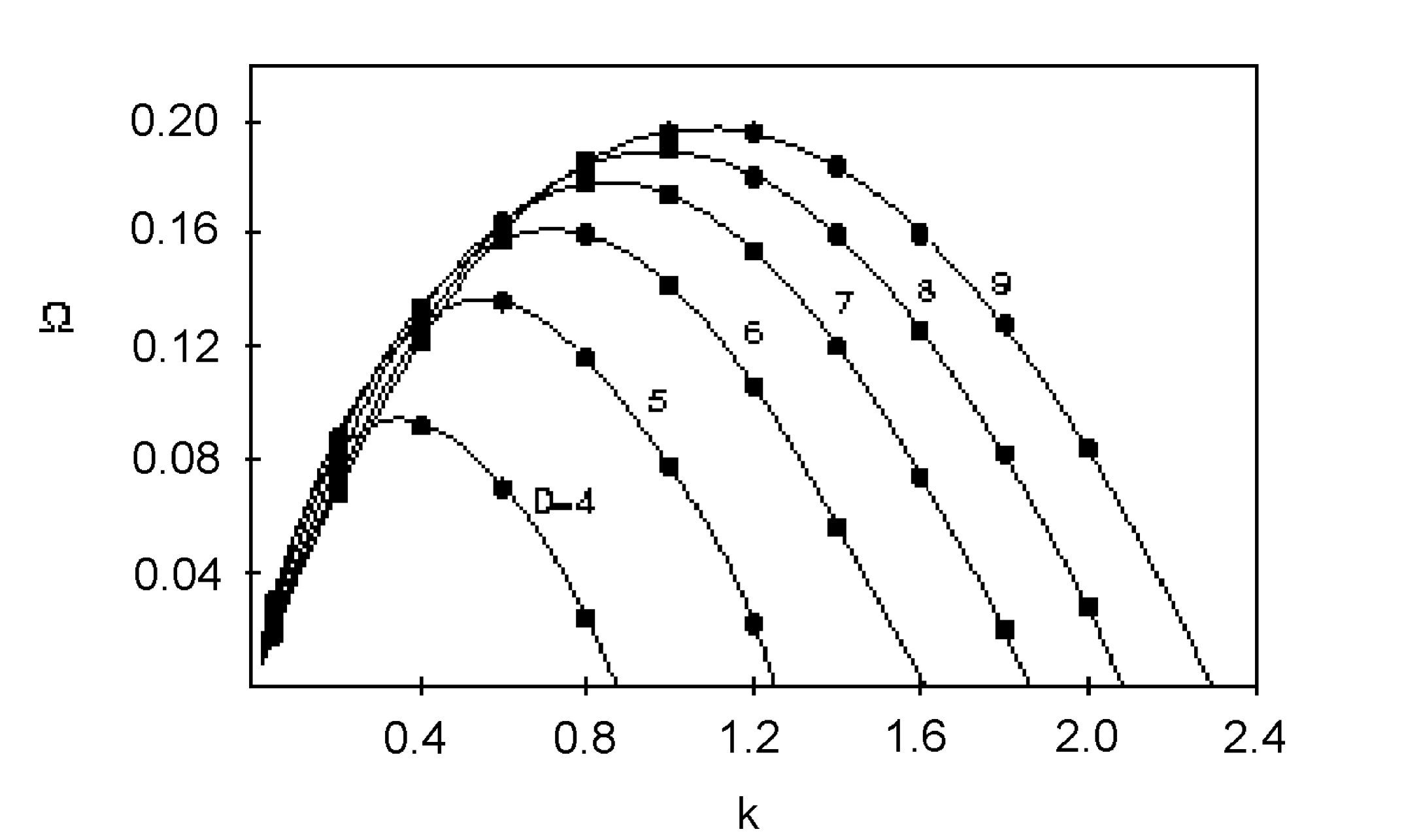
Figure 1: The Gregory-Laflamme $\Omega(k)$ curve in $D+1=10-p$ dimensions. Reprinted from Ref. [2].

4.2 Non-extremal smeared D$p$-branes

In Section 2.1 we reviewed the boost/U-duality transformation of [20] that takes a neutral black string to a D$p$-brane solution smeared on a transverse direction. In this section we describe the transformation that takes the unstable GL mode of the neutral black string to an unstable mode of the non-extremal D$p$-brane solution smeared on a transverse circle.

The transformation should convert the neutral black string solution (2.2) to the smeared D$p$-brane solution (2.5). If we try naively to apply the boost/U-duality transformation reviewed in Section 2.1 to the GL mode (4.1) we find a non-normalizable exponential dependence on $y$ (the critical case $k=k_{c}$ is an exception). As was pointed out in [22], to avoid this problem we may consider a complex metric perturbation, and try to find a complex transformation that i) Gets rid of the exponential $y$ dependence, ii) Still has the same effect on the zeroth order part of the metric, $i.e.$ on the neutral black string metric. At the end one can take the real part of the transformed perturbation. Note that this last step works only because of the linearity of the perturbed Einstein equations of motion.

The precise form of the transformation we look is as follows. First define the coordinates $\tilde{y}$ and $z^{\prime}$ by the following complex rotation of the $y$ and $z$ coordinates

$$\left(\begin{array}[]{c}y^{\prime}\\ \tilde{z}\end{array}\right)=M\left(\begin{array}[]{c}y\\ z\end{array}\right)\ ,\ \ M=\left(\begin{array}[]{cc}\cosh w&-i\sinh w\\ i\sinh w&\cosh w\end{array}\right)\ .$$ (4.3)

Notice that the neutral black string metric (2.2) embedded in eleven dimensional gravity is invariant under (4.3) since $(dy^{\prime})^{2}+(d\tilde{z})^{2}=dy^{2}+dz^{2}$. The transformation (4.3) is then supplemented by a boost that takes the $(t,y^{\prime})$ coordinates to the $(\tilde{t},\tilde{y})$ coordinates given by

$$\left(\begin{array}[]{c}\tilde{t}\\ \tilde{y}\end{array}\right)=\Lambda\left(\begin{array}[]{c}t\\ y^{\prime}\end{array}\right)\ ,\ \ \Lambda=\left(\begin{array}[]{cc}\cosh\alpha&\sinh\alpha\\ \sinh\alpha&\cosh\alpha\end{array}\right)~{}.$$ (4.4)

These rotations are such that

$$\sinh w=\frac{\Omega}{k}\tanh\alpha\ ,\ \ \tilde{k}=k\cosh w\ ,\ \ \tilde{\Omega}=\frac{\Omega}{\cosh\alpha}~{}.$$ (4.5)

Then we can write the real part of the boosted perturbation of the eleven dimensional metric (2.4) as

$$\tilde{h}_{\mu\nu}=\mbox{Re}\left\{\exp\left(\frac{\tilde{\Omega}t}{r_{0}}+i\frac{\tilde{k}z}{r_{0}}\right)\tilde{P}_{\mu\nu}\right\}~{}.$$ (4.6)

Using the relation $\tilde{P}=\Lambda^{-1}M^{-1}P(M^{-1})^{T}(\Lambda^{-1})^{T}$ we find

$$\begin{array}[]{c}\displaystyle\tilde{P}_{tt}=-f\psi\cosh^{2}\alpha\ ,\ \ \tilde{P}_{yy}=-f\psi\sinh^{2}\alpha\ ,\ \ \tilde{P}_{ty}=f\psi\sinh\alpha\cosh\alpha\ ,\\[8.53581pt] \displaystyle\tilde{P}_{tr}=\eta\cosh\alpha\ ,\ \ \tilde{P}_{yr}=-\eta\sinh\alpha\ ,\ \ \tilde{P}_{rr}=f^{-1}\chi\ ,\ \ \tilde{P}_{\rm sphere}=r^{2}\kappa~{},\end{array}$$ (4.7)

where we have made the relabellings $\tilde{t}\rightarrow t$ and $\tilde{y}\rightarrow y$. Notice that the complex rotation (4.3) precisely ensures that the exponential factor does not have a $y$-dependence. We can therefore apply the same U-duality transformations on (4.6)-(4.7) as on the boosted neutral black string. After these U-duality transformations, consisting of one S-duality and $p$ T-dualities, we conclude that the perturbed non-extremal D$p$-brane smeared on a transverse direction can be written as

$$\begin{array}[]{c}\displaystyle\begin{array}[]{rcl}ds^{2}&=&\displaystyle H_{\rm c}^{-1/2}\left[-f_{\rm c}dt^{2}+\sum_{i=1}^{p}dx_{i}^{2}+2\eta\cosh\alpha{\cal E}dtdr\right]\\[14.22636pt] &&\displaystyle+H_{\rm c}^{1/2}\Big{[}f^{-1}(1+\chi{\cal E})dr^{2}+dz^{2}+r^{2}(1+\kappa{\cal E})d\Omega_{7-p}^{2}\Big{]}\ ,\end{array}\\[34.1433pt] \displaystyle e^{2\phi}=H_{\rm c}^{(3-p)/2}\ ,\ \ A_{01\cdots p}=\coth\alpha(H_{\rm c}^{-1}-1)\ ,\ \ A_{r1\cdots p}=-H^{-1}\eta\sinh\alpha{\cal E}\ ,\\[8.53581pt] \displaystyle f=1-\frac{r_{0}^{6-p}}{r^{6-p}}\ ,\ \ H=1+\sinh^{2}\alpha(1-f)\ ,\ \ f_{\rm c}\equiv f(1+\psi{\cal E})\ ,\ \ H_{\rm c}\equiv 1+\sinh^{2}\alpha(1-f_{\rm c})\ ,\\[8.53581pt] \displaystyle{\cal E}=\cos\left(\tilde{k}r_{0}^{-1}z\right)\exp\left(\tilde{\Omega}r_{0}^{-1}t\right)\ .\end{array}$$ (4.8)

The perturbed D$p$-brane background appears here in one compact expression. From this one can easily deduce the explicit form of the perturbation by expanding to first order. The unstable mode appearing in [22] is equivalent to (4.8) for $p=0$, though written in a different gauge.

Note that the functions $\psi$, $\eta$, $\chi$ and $\kappa$ are still solutions to Eqs. (A.7)-(A.15) with $f$ given by (A.2). In particular $\psi$ is a solution of Eq. (4.2). All of these functions depend on the variable $x=rk/r_{0}$ just as in the case of the neutral black string perturbation.

Furthermore, we see from (4.5) that $\tilde{k}^{2}=k^{2}+\Omega^{2}\tanh^{2}\alpha$ and $\tilde{\Omega}=\Omega/\cosh\alpha$. Hence, we can obtain $\tilde{\Omega}$ as function of $\tilde{k}$ by using the functional dependence $\Omega(k)$ for the neutral black string (as sketched for $p=0,...,5$ in Figure 1). We note that the critical point $(k,\Omega)=(k_{c},0)$ is mapped to the critical point $(\tilde{k},\tilde{\Omega})=(k_{c},0)$, which corresponds to the marginal mode of the D$p$-brane with a transverse direction. This marginal mode appears at the origin of the non-uniform phase of non-extremal D$p$-branes with a transverse direction [20]. From Figure 1 we also deduce that $\tilde{k}<k_{c}$ for any $k<k_{c}$ and the function $\tilde{\Omega}(\tilde{k})$ never exhibits time-dependent modes with wavelength smaller than the critical one.

The existence of the perturbation (4.8) proves explicitly that a non-extremal D$p$-brane with a transverse flat direction is always unstable as a gravitational background. This result meshes nicely with the unstable thermodynamics in (2.18), (2.19) and confirms the validity of the CSC if we consider it in the grand canonical ensemble. In contrast to this, a D$(p+1)$-brane wrapped on the T-dual $z$-circle is known to be classically stable in supergravity close to extremality. This fact is in agreement with the CSC if we consider it in the canonical ensemble (see (2.18)).

4.3 Near-extremal limit

We now consider the near-extremal limit (2.9) of the unstable mode (4.8) for non-extremal D$p$-branes with a transverse direction. The near-extremal limit of the unperturbed non-extremal solutions (2.5) has been discussed already in Section 2, giving the near-extremal D$p$-brane background (2.10).

Applying the limit (2.9) on the background (4.8) gives the following perturbation of the near-extremal D$p$-brane (2.10)

$$\begin{array}[]{c}\begin{array}[]{rcl}l_{s}^{-2}ds^{2}&=&\displaystyle\hat{H}_{\rm c}^{-1/2}\left[-f_{\rm c}dt^{2}+\sum_{i=1}^{p}dx_{i}^{2}+2\eta\sqrt{K}u_{0}^{p/2-3}{\cal E}dtdu\right]\\[14.22636pt] &&\displaystyle+\hat{H}_{\rm c}^{1/2}\Big{[}f^{-1}(1+\chi{\cal E})du^{2}+d\hat{z}^{2}+u^{2}(1+\kappa{\cal E})d\Omega_{7-p}^{2}\Big{]}\ ,\end{array}\\[34.1433pt] \displaystyle e^{2\phi}=\hat{H}_{\rm c}^{(3-p)/2}\ ,\ \ A_{01\cdots p}=\hat{H}_{\rm c}^{-1}\ ,\ \ A_{r1\cdots p}=-u^{6-p}K^{-1/2}u_{0}^{p/2-3}\eta{\cal E}\ ,\\[8.53581pt] \displaystyle f=1-\frac{u_{0}^{6-p}}{u^{6-p}}\ ,\ \ f_{\rm c}=f(1+\psi{\cal E})\ ,\ \ \hat{H}_{\rm c}=\frac{K}{u^{6-p}}\left[1-\left(\frac{u^{6-p}}{u_{0}^{6-p}}-1\right)\psi{\cal E}\right]\ ,\\[11.38109pt] \displaystyle{\cal E}=\cos\left(\sqrt{k^{2}+\Omega^{2}}\frac{\hat{z}}{u_{0}}\right)\exp\left(u_{0}^{2-\frac{1}{2}p}K^{-1/2}\Omega t\right)\ .\end{array}$$ (4.9)

We note that the near-extremal limit (2.9) keeps $k$ and $\Omega$ fixed, and moreover keeps $\psi$, $\eta$, $\chi$ and $\kappa$ fixed as functions of the variable $x$ which is now given by

$$x=\frac{uk}{u_{0}}\ .$$ (4.10)

Therefore, the functions $\psi$, $\eta$, $\chi$ and $\kappa$ are still solutions of the Eqs. (A.7)-(A.15) with $f$ given by (A.2). In particular $\psi$ is still a solution of Eq. (4.2).

We have thus shown that the near-extremal limit of the time-dependent mode of smeared branes is well-defined and hence that near-extremal smeared D$p$-branes are classically unstable. Then according to the CSC this means that near-extremal D$p$-branes should be thermodynamically unstable in the grand canonical ensemble. However, as noted in Section 2.2, we do not have a priori a definition of this ensemble for near-extremal branes, since it seems that the charge cannot vary anymore. We will resolve this puzzle in Section 6, where we will show that there does exist an appropriate definition of this ensemble in the near-extremal limit. We will see that in this ensemble near-extremal smeared D$p$-branes are indeed thermodynamically unstable, in accordance with the above result and the CSC.

5 Connection to marginal modes of extremal smeared branes

In this section we find a connection between the GL mode of charged smeared branes described in Section 4 and the marginal modes of extremal smeared branes.

5.1 Marginal modes for extremal smeared branes

In general, the solutions for extremal D$p$-branes distributed along a single flat direction $z$ is given as

$$\begin{array}[]{c}\displaystyle ds^{2}=H^{-1/2}\left(-dt^{2}+\sum_{i=1}^{p}dx_{i}^{2}\right)+H^{1/2}\left(dr^{2}+dz^{2}+r^{2}d\Omega_{7-p}^{2}\right)\ ,\\[14.22636pt] \displaystyle e^{2\phi}=H^{(3-p)/2}\ ,\ \ A_{01\cdots p}=H^{-1}-1\ ,\end{array}$$ (5.1)

where the harmonic function $H(r,z)$ obeys

$$\left(\partial_{r}^{2}+\frac{7-p}{r}\partial_{r}+\partial_{z}^{2}\right)H(r,z)=0\ ,$$ (5.2)

away from the source distribution. Given the appropriate boundary conditions the general solution is

$$H(r,z)=1+\int_{-\infty}^{\infty}dz^{\prime}\frac{\rho(z^{\prime})}{(r^{2}+(z-z^{\prime})^{2})^{(7-p)/2}}\ ,$$ (5.3)

where the charge distribution function $\rho(z)$ is arbitrary. Now, the extremal smeared D$p$-brane case corresponds obviously to $\rho$ being constant. But, it is clearly possible to add to the constant charge distribution a single mode of any wave-number $q$, in which case the harmonic function takes the form

$$H=1+\frac{Kl_{s}^{8-2p}}{r^{6-p}}+m(qr)\cos(qz)\ ,$$ (5.4)

where $K$ is defined in (2.7) and the function $m(qr)$ solves

$$m^{\prime\prime}(y)+\frac{7-p}{y}m^{\prime}(y)-m(y)=0\ .$$ (5.5)

The solutions of Eq. (5.5) are of the form $m(y)\propto y^{-(6-p)/2)}{\cal{K}}_{(6-p)/2}(y)$, ${\cal{K}}_{s}(y)$ being the modified Bessel function of the second kind. The modes given by (5.4) are marginal in the sense that the modified solution solves the supergravity equations. In this sense the extremal smeared branes have marginal modes of any wave-length.

It is interesting to consider what happens to such marginal modes if one perturbs the extremal brane so that it gets a temperature. This is one of the things which we address in Section 5.2. Clearly from the study of non-extremal D$p$-branes distributed on transverse directions, one does not expect the existence of static solutions for any charge distribution $\rho(z)$. This is one example where gravity behaves vastly different from, say, electromagnetism where solutions with arbitrary charge distributions exist, although most of them are not stable when interactions are taken into account.

Since we shall explore in the following a connection with near-extremal branes, we need to consider briefly the near-horizon limit (2.9) of the extremal D$p$-brane background given by (5.1) and (5.4). This gives

$$\begin{array}[]{c}\displaystyle l_{s}^{-2}ds^{2}=\hat{H}^{-1/2}\left(-dt^{2}+\sum_{i=1}^{p}dx_{i}^{2}\right)+\hat{H}^{1/2}\left(du^{2}+d\hat{z}^{2}+u^{2}d\Omega_{7-p}^{2}\right)\ ,\\[5.69054pt] \displaystyle e^{2\phi}=\hat{H}^{(3-p)/2}\ ,\ \ A_{01\cdots p}=\hat{H}^{-1}\ ,\ \ \hat{H}=\frac{K}{u^{6-p}}+m(qu)\cos(q\hat{z})\ .\end{array}$$ (5.6)

Note that the function $m(qu)$ has been rescaled appropriately, and that $m(y)$ still obeys Eq. (5.5).

5.2 Extremal limit of the Gregory-Laflamme perturbation

In this section we consider the extremal limit of the GL mode for near-extremal smeared D$p$-branes, as found in Section 4.3. As we see in a moment, this gives a connection between the marginal modes of extremal smeared branes considered in Section 5.1 and the GL modes of near-extremal smeared branes.

Let us take the extremal limit of the perturbation of near-extremal D$p$-branes smeared on a transverse direction, as given by (4.9). The extremal limit corresponds to $u_{0}\rightarrow 0$ with $u$ and $K$ kept fixed. We first remark that since we want the argument of the cosine factor to remain finite, we need $\sqrt{k^{2}+\Omega^{2}}/u_{0}$ to stay finite in the limit. Hence, we need $k/u_{0}$ and $\Omega/u_{0}$ to remain fixed in the limit $u_{0}\rightarrow 0$. In terms of the dispersion diagram of Figure 1 this means that we move closer and closer to the point $(k,\Omega)=(0,0)$ on the left part of the curve. We see that the variable $x=uk/u_{0}$ defined above stays finite in the limit. Note also that this limit necessarily has the consequence that the time-dependent exponential factor in ${\cal E}$ in (4.9) disappears. One can now see from $\hat{H}_{c}$ in (4.9) that we need $\psi(x)/u_{0}^{6-p}$ to stay finite. By using this in Eqs. (A.3)-(A.15) and demanding consistency of this system of equations, we get similar conditions on $\eta$, $\chi$ and $\kappa$, so that in total the extremal limit is given as

$$u_{0}\rightarrow 0\ \mbox{ with }\ u\ ,\ K\ ,\ \frac{k}{u_{0}}\ ,\ \frac{\Omega}{u_{0}}\ ,\ \frac{\psi(x)}{u_{0}^{6-p}}\ ,\ \frac{\eta(x)}{u_{0}^{6-p}}\ ,\ \frac{\chi(x)}{u_{0}^{6-p}}\ ,\ \frac{\kappa(x)}{u_{0}^{6-p}}\ \mbox{ kept fixed}\ .$$ (5.7)

Applying the extremal limit (5.7) to the perturbed near-extremal solution given in (4.9), we get the following background

$$\begin{array}[]{c}\begin{array}[]{rcl}l_{s}^{-2}ds^{2}&=&\displaystyle\hat{H}_{\rm c}^{-1/2}\left[dt^{2}+\sum_{i=1}^{p}dx_{i}^{2}\right]+\hat{H}_{\rm c}^{1/2}\Big{[}du^{2}+d\hat{z}^{2}+u^{2}d\Omega_{7-p}^{2}\Big{]}\ ,\end{array}\\[11.38109pt] \displaystyle e^{2\phi}=\hat{H}_{\rm c}^{(3-p)/2}\ ,\ \ A_{01\cdots p}=\hat{H}_{\rm c}^{-1}\ ,\ \ \hat{H}_{\rm c}=\frac{K}{u^{6-p}}-\frac{\psi}{u_{0}^{6-p}}{\cal E}\ ,\\[11.38109pt] \displaystyle{\cal E}=\cos\left(\frac{\sqrt{k^{2}+\Omega^{2}}}{u_{0}}\hat{z}\right)\ .\end{array}$$ (5.8)

We see that out of the four functions $\psi$, $\eta$, $\chi$ and $\kappa$ making up the near-extremal GL mode only $\psi$ survives. Moreover, the equation (4.2) for $\psi(x)$ becomes

$$\psi^{\prime\prime}(x)+\frac{7-p}{x}\psi^{\prime}(x)-\bigg{(}1+\frac{\Omega^{2}}{k^{2}}\bigg{)}\psi(x)=0~{}.$$ (5.9)

We deduce that the background (5.8) precisely corresponds to the background (5.6) describing a extremal smeared D$p$-brane perturbed by a marginal mode with the wave-number

$$q=\frac{\sqrt{k^{2}+\Omega^{2}}}{u_{0}}\ .$$ (5.10)

In particular, one can check explicitly that the $\psi$ equation (5.9) turns into Eq. (5.5) by identifying $m(qu)=\psi(ku/u_{0})$. This means that the extremal limit of the GL mode becomes stable as also observed for unsmeared black branes in Ref. [11].

It is easy to see that we can get marginal modes of any wave-number. For small $k$ we have $\Omega=\gamma k$, where $\gamma$ is an appropriate number. Therefore, $q=\sqrt{1+\gamma^{2}}k/u_{0}$, and by choosing $k/u_{0}$ we can get any value of $q$ that we want. We have thus shown that in the extremal limit the GL modes of the near-extremal smeared branes precisely become the marginal modes of extremal smeared branes. This answers the question posed in Section 5.1 of what happens to a marginal mode of an extremal smeared brane when perturbing the background so that it turns non-BPS: The mode will turn into the near-extremal GL mode (4.9). Obviously, this has the consequence that the brane background is classically unstable and it will therefore decay.

Moreover, one can imagine having a charge distribution of the form

$$\rho=\rho_{0}+\sum_{n\neq 0}\rho_{n}\cos(q_{n}\hat{z})\ ,$$ (5.11)

where $\rho_{n}$ are small compared to $\rho_{0}$. When we make a non-BPS perturbation this solution involves a sum over GL modes which is of the form

$$h_{\mu\nu}=\sum_{n\neq 0}h^{(n)}_{\mu\nu}(u)\cos(q_{n}\hat{z})\exp\left(\frac{\gamma u_{0}^{3-\frac{p}{2}}}{\sqrt{K}\sqrt{1+\gamma^{2}}}q_{n}t\right)\ ,$$ (5.12)

for $u_{0}$ being small. In this way we can find a non-BPS continuation of any extremal perturbation of the extremal smeared branes, since we can fourier decompose the perturbation and put it in the form (5.11).

It is important to note that the connection between the marginal modes of extremal smeared branes and the GL modes of near-extremal branes easily generalizes to a connection with GL modes of non-extremal branes. We choose for convenience here only to consider the connection to near-extremal branes.

The physical consequence of the connection between marginal modes of the extremal smeared branes and the GL mode of the non- and near-extremal smeared branes is that extremal smeared branes are in a sense arbitrarily close to being unstable. Therefore, if one imagined a practical application of extremal smeared branes one would run into the problem that any disturbance of the background which is non-BPS would cause the whole background to destabilize and decay. Also, this feature of extremal smeared branes makes it very unlikely that they form in any cosmologic scenario, even though they are stable by themselves.

6 The CSC for near-extremal branes

In this section, we return to the puzzle alluded to at the end of Section 2.2 and further commented on at the end of Section 4.3. We have seen in Section 4.3, by applying boost/U-duality and the near-extremal limit, that near-extremal smeared branes are classically unstable. According to the CSC this classical instability should be related to thermodynamic instability in the grand canonical ensemble, when taking the near-extremal limit. On the other hand, we observed in Section 2.2 that in the near-extremal limit we have $C_{Q}>0$ and $c=0$ for near-extremal smeared branes, suggesting marginal thermodynamic stability. This seems to be in contradiction with the CSC.

The resolution of the puzzle is that in the near-extremal limit one should not compute the quantity $c$ using the non-extremal chemical potential $\nu$, but using a new chemical potential $\hat{\nu}$, which can be understood roughly as the “chemical potential above extremality”. This is in analogy to the fact that we do not compute $C_{Q}$ using the mass $M$ (which goes to infinity in the near-extremal limit), but using the energy $E$ above extremality, which is finite.

To derive the expression for $\hat{\nu}$, we note that the first law of thermodynamics for non-extremal branes takes the form

$$dE=TdS+(\nu-1)dQ\ ,$$ (6.1)

when written in terms of $E=M-Q$. Moreover, one can easily see from (2.11), that the chemical potential $\nu$ approaches 1 in the near-extremal limit $\alpha\rightarrow\infty$, and is not a free parameter anymore. It is therefore natural to define the rescaled chemical potential $\hat{\nu}$ and the corresponding rescaled charge ${\hat{Q}}$ as

$$\hat{\nu}\equiv\frac{1}{g_{\mathrm{YM}}^{2}}\lim_{l_{s}\rightarrow 0}\frac{1}{l_{s}^{4}}(\nu-1)\ ,\ \ \hat{Q}\equiv g_{\mathrm{YM}}^{2}\lim_{l_{s}\rightarrow 0}l_{s}^{4}Q\ ,$$ (6.2)

where the factor of $l_{s}$ has been chosen such that $\hat{\nu}$ is finite in the near-extremal limit. The finite factor $g_{\mathrm{YM}}^{2}$ has been inserted for later convenience. With the definitions (6.2), we then find that (6.1) can be written as

$$dE=TdS+\hat{\nu}d\hat{Q}\ ,$$ (6.3)

which is a well-defined differential relation in the near-extremal limit. We have thus obtained a new version of the first law of thermodynamics for near-extremal branes involving an extra term containing the rescaled chemical potential $\hat{\nu}$ and rescaled charge $\hat{Q}$.

In further detail, using the non-extremal quantities (2.11) and the near-extremal limit (2.9) in the definitions (6.2) we find for near-extremal smeared D$p$-branes the expressions

$$\hat{Q}=(6-p)\frac{K}{{\cal{G}}}\ ,\ \ \hat{\nu}=-\frac{u_{0}^{6-p}}{2K}\ ,$$ (6.4)

where $K$ and ${\cal{G}}$ are defined in (2.7), (2.8).

The near-extremal Gibbs free energy is then naturally defined by $G(T,\hat{\nu})=E-TS-\hat{\nu}\hat{Q}$, and the condition for thermodynamic stability of near-extremal smeared branes in the grand canonical ensemble follows immediately by analogy with (2.16), namely

$$C_{\hat{Q}}=\left(\frac{\partial E}{\partial T}\right)_{\hat{Q}}>0\ ,\ \ \hat{c}=\left(\frac{\partial\hat{\nu}}{\partial\hat{Q}}\right)_{T}>0\ .$$ (6.5)

Computing these quantities for near-extremal smeared D$p$-branes, we find that the quantity $C_{\hat{Q}}$ is identical to the one computed in (2.21). On the other hand, for $\hat{c}$ we find using (6.4) and (2.12) after some algebra that

$$\hat{c}=-\frac{{\cal{G}}}{g_{\rm YM}^{4}K^{2}}\frac{u_{0}^{6-p}}{(4-p)(6-p)}\ ,$$ (6.6)

which is finite and negative for $p\leq 3$. As a consequence we find that near-extremal smeared D$p$-branes with $p\leq 3$ are thermodynamically unstable in the near-extremal grand canonical ensemble defined above, in agreement with the classical stability analysis and the CSC.

Interpretation in the dual gauge theory

Using (2.7), (2.8) in (6.4) we can express $\hat{\nu}$ and $\hat{Q}$ in gauge theory variables. The result is

$$\hat{Q}=\frac{\bar{L}V_{p}}{(2\pi)^{2}}N\ ,\ \ \hat{\nu}=-\frac{6-p}{2}\Omega_{7-p}(2\pi)^{2p-7}\frac{u_{0}^{6-p}}{g_{\mathrm{YM}}^{4}N}\ .$$ (6.7)

These quantities have a natural interpretation in the dual gauge theory. In the presence of the spatial circle the gauge theory possesses a non-trivial spatial Wilson loop. $\hat{Q}$ is naturally related to the number of eigenvalues of this operator and $\hat{\nu}$ is the corresponding chemical potential. Hence, the GL instabilities that we found previously within supergravity translate in gauge theory into a new set of phase transitions parametrized by the Wilson loop around the spatial circle. A recent discussion of these transitions in 0+1 and 1+1 dimensions appeared in [22] both at weak and strong coupling.

In the present work we have seen that a near-extremal D$p$-brane smeared on a transverse circle exhibits a momentum mode instability when the radius of the circle becomes sufficiently large. The smeared D$p$-brane is T-dual to a D$(p+1)$-brane on which the dual gauge theory lives. In the T-dual picture the near-extremal D$(p+1)$-brane exhibits a winding mode instability along a longitudinal circle when the T-dual radius is sufficiently small. From the string theory point of view the condensation of the unstable winding mode will be a dynamical process from the usual D$(p+1)$-brane phase to a non-trivial D$(p+1)$-brane phase which is T-dual to the localized phase of the D$p$-brane.

We can examine what this means on the gauge theory side. For example when considering smeared D2-branes, the above picture suggests that by perturbing $N=4$ $D=4$ SYM on a spatial circle for small temperatures with a particular type of relevant operator the theory destabilizes and eventually settles down to a phase in which it behaves approximately as the 2+1 dimensional SYM theory obtained by dimensional reduction of the $N=4$ $D=4$ SYM theory. Similar statements apply to gauge theories on the world-volume of other D$p$-branes. It would be interesting to examine this type of process more closely.

7 Conclusions

In this paper we considered non-extremal and near-extremal D$p$-branes smeared on a transverse direction. These branes exhibit GL instabilities, which can be obtained most easily from GL instabilities of neutral branes by a suitable boost/U-duality map. We showed explicitly that the unstable modes persist in the near-extremal limit and reduce to the more standard marginal modes of the extremal smeared branes, when we further take the extremal limit. This picture meshes nicely with the picture suggested by a local thermodynamic stability analysis when we apply the correlated stability conjecture in the grandcanonical ensemble. As we saw, a natural definition of such an ensemble exists also in the near-extremal limit. Moreover, for this class of smeared D$p$-branes we provided a proof of the CSC by extending previous arguments of Reall [9].

There is a number of further interesting issues related to the above circle of ideas. One of them has to do per se with the CSC. So far, there has been no general and complete proof of this conjecture. It would be interesting to generalize the arguments presented here to a wider class of systems, for example to systems of bound states. In general, the CSC appears to be such a natural conjecture that one may wonder whether it is possible to find a proof based on a more universal argument (see [37] for work in this direction). In cases where the CSC is violated [18] it would be interesting to examine possible ways in which it can be restricted or revised accordingly.

In this note we treated standard unstable GL modes with non-vanishing momentum and zero winding. A T-duality transformation converts the smeared brane into a wrapped brane. In string theory, the wrapping brane continues to be unstable, but now the unstable mode has non-vanishing winding. The winding state in question is expected to become tachyonic when the (T-dual) radius is smaller than the critical value. It would be very interesting to explore situations in string theory where the presence and dynamics of this mode can be analyzed explicitly.

Because of the AdS/CFT correspondence each of the above phenomena has some counterpart in the dual gauge theory. In particular, the GL instabilities translate into a new set of phase transitions with order parameters associated to the Wilson loops around the non-trivial cycles of the spacetime of the gauge theory. For a recent examination of this type of transitions in 0+1 and 1+1 dimensions see [22, 40]. The rescaled “charge” $\hat{Q}$ is naturally related to the number of eigenvalues of the spatial Wilson loop observables mentioned just above and the near-extremal quantity $\hat{\nu}$ is just the corresponding chemical potential. In gravity the phase transition to a localized phase is a dynamical process from a black string phase to a black hole phase. It would be interesting to obtain a better understanding of the dynamics of this process in gauge theory.

Appendix A The Gregory-Laflamme mode

We consider here the GL instability [2, 3] for the metric (2.1) corresponding to a uniform black string in $10-p$ dimensions. The instability is given by the metric perturbation $h_{\mu\nu}$ in the sense that $g_{\mu\nu}+h_{\mu\nu}$ is the black string metric plus perturbation. The perturbation $h_{\mu\nu}$ appears in (4.1). In (4.1) $\psi$, $\eta$, $\chi$ and $\kappa$ are all functions of the variable

$$x=\frac{rk}{r_{0}}\ ,$$ (A.1)

and this is the variable that we take derivatives with respect to. The function $f$ is given in terms of $x$ by

$$f=1-\frac{k^{6-p}}{x^{6-p}}\ .$$ (A.2)

The tracelessness conditions are

$$(7-p)\kappa+\chi+\psi=0\ .$$ (A.3)

The transversality condition is

$$\begin{array}[]{c}\displaystyle\frac{\Omega}{k}x\psi+(6-p)(1-f)\eta+f\left((7-p)\eta+x\eta^{\prime}\right)=0\ ,\\[8.53581pt] \displaystyle-2\frac{\Omega}{k}x\eta+(6-p)(1-f)(\chi-\psi)+2f\left((8-p)\chi+\psi+x\chi^{\prime}\right)=0\ .\end{array}$$ (A.4)

The four independent Einstein equations take the form

$$\displaystyle\begin{array}[]{l}\displaystyle x\frac{\Omega}{k}\psi+(6-p)(1-f)\eta+\frac{k}{\Omega}f^{2}\big{(}(7-p)\psi^{\prime}+x\psi^{\prime\prime}\big{)}\\[5.69054pt] \displaystyle+f\left[2(7-p)\eta-x\frac{k}{\Omega}\psi+2x\eta^{\prime}+\frac{k}{\Omega}(6-p)(1-f)(-\chi^{\prime}+\psi^{\prime})\right]=0~{},\end{array}$$ (A.7)

$$\displaystyle-(6-p)(1-f)x\frac{\Omega}{k}(\chi+\psi)+2f\left[x\frac{\Omega}{k}((8-p)\chi+\psi+x(\chi^{\prime}+\psi^{\prime}))+\eta x^{2}\right]=0~{},~{}~{}$$ (A.8)

$$\displaystyle\begin{array}[]{l}\displaystyle x^{2}\bigg{(}\frac{\Omega^{2}}{k^{2}}+f\bigg{)}\chi-(6-p)(1-f)\frac{\Omega}{k}x\eta\\[11.38109pt] \displaystyle+f\left[-2x^{2}\frac{\Omega}{k}\eta^{\prime}+(6-p)(1-f)x(\chi^{\prime}-\psi^{\prime})+xf\big{(}(9-p)\chi^{\prime}+2\psi^{\prime}+x\chi^{\prime\prime}\big{)}\right]=0~{},\end{array}$$ (A.11)

$$\displaystyle\begin{array}[]{l}f\bigg{[}\psi\big{(}-x^{2}+2(6-p)(1-f)\big{)}+\chi\big{(}-x^{2}+2(8-p)(6-p)(1-f)\big{)}\\ \displaystyle-2(7-p)x\frac{\Omega}{k}\eta+(6-p)(1-f)x(\chi^{\prime}+\psi^{\prime})\bigg{]}+f^{2}\bigg{[}2(8-p)(6-p)\chi\\ \displaystyle+2(6-p)\psi+x\big{(}3(7-p)\chi^{\prime}+(7-p)\psi^{\prime}+x(\chi^{\prime\prime}+\psi^{\prime\prime})\big{)}\bigg{]}-x^{2}\frac{\Omega^{2}}{k^{2}}(\chi+\psi)=0~{}.\end{array}$$ (A.15)

Combining the gauge conditions (A.3)-(A.4) with the Einstein equations (A.7)-(A.15) one can derive Eq. (4.2) which is a second order differential equation for $\psi$ of the form

$$\psi^{\prime\prime}(x)+{\cal Q}_{p}(x)\psi^{\prime}(x)+{\cal P}_{p}(x)\psi(x)=0~{}.$$ (A.16)

${\cal Q}_{p}$ and ${\cal P}_{p}$ are $p$-dependent rational functions of $x$, which we summarize here for completeness

$${\cal Q}_{p}(x) = f^{-1}x^{-1}\Big{[}f^{3}k^{4}(372-64p+3p^{2})+\Omega^{2}\big{(}k^{2}(p-6)^{2}-4\Omega^{2}\big{)}$$ (A.17)

$$+k^{2}f^{2}\big{(}k^{2}(44+4p-2p^{2})+3(p-14)(3p-22)\Omega^{2}\big{)}$$

$$-k^{2}f\big{(}k^{2}(p-6)^{2}+2(292-78p+5p^{2})\Omega^{2}\big{)}\Big{]}^{-1}$$

$$\times\Big{[}k^{4}f^{4}(-108+124p-21p^{2}+p^{3})-3(p-6)\Omega^{2}\big{(}k^{2}(p-6)^{2}-4\Omega^{2}\big{)}$$

$$+k^{2}f^{2}\big{(}k^{2}(p-6)(-62+5p+p^{2})+\Omega^{2}(11152-4680p+656p^{2}-31p^{3})\big{)}$$

$$+k^{2}f^{3}\big{(}k^{2}(2828-964p+106p^{2}-4p^{3})+\Omega^{2}(-2412+1120p-165p^{2}+8p^{3})\big{)}$$

$$f\big{(}2k^{4}(p-6)^{3}+k^{2}\Omega^{2}(p-6)(1126-341p+26p^{2})+4(11-2p)\Omega^{4}\big{)}\Big{]}~{},$$

$${\cal P}_{p}(x) = k^{-2}f^{-2}x^{-2}\Big{[}f^{3}k^{4}(372-64p+3p^{2})+\Omega^{2}\big{(}k^{2}(p-6)^{2}-4\Omega^{2}\big{)}$$ (A.18)

$$+k^{2}f^{2}\big{(}k^{2}(44+4p-2p^{2})+3(p-14)(3p-22)\Omega^{2}\big{)}$$

$$-k^{2}f\big{(}k^{2}(p-6)^{2}+2(292-78p+5p^{2})\Omega^{2}\big{)}\Big{]}^{-1}$$

$$\times\Big{[}-2k^{6}f^{5}(p-8)^{2}(p-6)^{2}+k^{4}f^{4}\big{(}k^{2}(8880-110p^{3}+4p^{4}-372x^{2}$$

$$-3p^{2}(-378+x^{2})+p(-5188+64x^{2}))-(p-6)^{2}(p-8)(-26+7p)\Omega^{2}\big{)}$$

$$-2k^{4}f^{3}\big{(}k^{2}(1956-26p^{3}+p^{4}+22x^{2}+2p(-577+x^{2})-p^{2}(-258+x^{2}))$$

$$+(-8448+206p^{3}-9p^{4}+708x^{2}+p(6340-144x^{2})+p^{2}(-1734+7x^{2}))\Omega^{2}\big{)}$$

$$+2fk^{2}\Omega^{2}\big{(}k^{2}(p-6)^{2}(-10-4p+p^{2}+x^{2})+(-84+606x^{2}+p(26-178x^{2})$$

$$+p^{2}(-2+13x^{2}))\Omega^{2}\big{)}+\Omega^{2}\big{(}k^{4}(p-6)^{4}-k^{2}(p-6)^{2}(-2+7x^{2})\Omega^{2}+4x^{2}\Omega^{4}\big{)}$$

$$+k^{2}f^{2}\big{(}k^{4}(p-6)^{2}(-10+2p+x^{2})-2k^{2}(4992-151p^{3}+7p^{4}-294x^{2}$$

$$-6p^{2}(-199+x^{2})+p(-4072+84x^{2}))\Omega^{2}+(96-1332x^{2}+p^{2}(2-19x^{2})$$

$$+4p(-7+80x^{2}))\Omega^{4}\big{)}\Big{]}~{}.$$

Appendix B An off-shell two-parameter family of black branes

In Section 3, we described a generalization of the proof of the correlated stability conjecture by adapting the analysis of [9] to the case of (smeared) black D$p$-branes in the grand canonical ensemble. Part of the argument involved the construction of an (off-shell) two-parameter family of Euclidean black branes. In this appendix we consider this construction in detail.

According to the discussion in Section 3 we need to construct a family of black-brane backgrounds with the property (3.3). The backgrounds of this family do not, in general, satisfy the equations of motion of general relativity, but they should satisfy the Hamiltonian constraint equations. This is a special subset of the full equations of motion. For pure gravity these constraints can be found, for example, in Eqs. (10.2.28), (10.2.30) of [43]. Our case involves a system of gravity coupled to a dilaton scalar field and a $(p+2)$-form gauge field strength. In the Einstein frame the action for this system is

$${\cal S}=\frac{1}{16\pi G}\int d^{10}x\sqrt{g}\bigg{[}-R+\frac{1}{2}(\partial\phi)^{2}+\frac{1}{2(p+2)!}e^{\alpha\phi}F^{2}_{(p+2)}\bigg{]}~{},$$ (B.1)

where $\alpha=\frac{3-p}{2}$. There are two Hamiltonian constraints for this system. They are

$$R_{00}-\frac{1}{2}Rg_{00}=\frac{1}{2}(\partial_{0}\phi)^{2}-\frac{1}{4}g_{00}(\partial\phi)^{2}+\frac{1}{2(p+1)!}e^{\alpha\phi}\bigg{(}F_{0\rho_{1}...\rho_{p+1}}F_{0}^{\rho_{1}...\rho_{p+1}}-\frac{1}{2(p+2)}F^{2}g_{00}\bigg{)}~{},$$ (B.2)

$$\nabla_{\mu}\bigg{(}e^{\alpha\phi}F^{\mu\rho_{1}...\rho_{p}0}\bigg{)}=0~{}.$$ (B.3)

The first constraint sets the total Hamiltonian to zero and the second is the Gauss constraint for the gauge field.

Assuming spherical symmetry let us write the generic point in the family as a background of the form

$$\begin{array}[]{c}\displaystyle ds^{2}=U(r)d\tau^{2}+V^{-1}(r)dr^{2}+S(r)\bigg{(}\sum_{i=1}dx_{i}^{2}+dz^{2}\bigg{)}+R(r)r^{2}d\Omega^{2}_{7-p}~{},\\[5.69054pt] \displaystyle e^{2\phi}=H(r)^{\frac{3-p}{2}}~{},~{}~{}F_{(p+2)}=F(r)dt\wedge dr\wedge dx_{1}\wedge\cdots\wedge dx_{p}~{}.\end{array}$$ (B.4)

The functions $U,V,S,R,H$ and $F$ should be such that the constraints (B.2), (B.3) are satisfied. Moreover, the family should include the on-shell smeared D$p$-branes (2.5) (transformed to the Einstein frame), for which

$$\begin{array}[]{c}\displaystyle U(r)=H(r)^{-\frac{7-p}{8}}f(r)~{},~{}~{}V(r)=H(r)^{-\frac{p+1}{8}}f(r)\ ,\ \ S(r)=R(r)=H(r)^{\frac{p+1}{8}}~{},\\[5.69054pt] \displaystyle F(r)=\coth\alpha\frac{d(H(r)^{-1})}{dr}\ ,\ \ f(r)=1-\frac{r_{0}^{6-p}}{r^{6-p}}~{},~{}~{}H(r)=1+\sinh\alpha\frac{r_{0}^{6-p}}{r^{6-p}}~{},\end{array}$$ (B.5)

in the Einstein frame.

It is straightforward to plug the ansatz (B.4) into the Hamiltonian constraints (B.2), (B.3) to get a pair of non-linear (second order and first order) differential equations for the functions $U,V,S,R,H$ and $F$. These complicated equations can be simplified considerably with the following ansatz

$$S(r)=R(r)~{},~{}~{}V(r)=-H(r)^{\frac{3-p}{4}}U(r)~{},$$ (B.6)

which is naturally suggested by the on-shell background (B.5). Then, one can solve easily the first order differential equation that comes from the Gauss constraint (B.3) to obtain the function $F(r)$ as a functional of the still arbitrary functions $H(r)$ and $S(r)$. The resulting expression is

$$F(r)=aH(r)^{\frac{p-3}{2}}S(r)^{p-4}r^{p-7}~{}.$$ (B.7)

Here $a$ is an integration constant that will be fixed appropriately below. Plugging this expression back into the differential equation that originates from (B.2) gives the differential equation

$$U^{\prime}(r)+P[H,S](r)U(r)+Q[H,S](r)=0~{},$$ (B.8)

where ^′ denotes differentiation with respect to $r$ and $P[H,S]$, $Q[H,S]$ are the following functionals of the still arbitrary functions $H$ and $S$

$$\begin{array}[]{rcl}P[H,S]&=&\bigg{[}-(\ln\Lambda)^{\prime\prime}-\frac{1}{4}\big{(}(\ln\Lambda)^{\prime}\big{)}^{2}+\frac{3-p}{4}(\ln H)^{\prime\prime}-\frac{(3-p)^{2}}{64}\big{(}(\ln H)^{\prime}\big{)}^{2}\\ &&-\frac{p+1}{4}\big{(}(\ln S)^{\prime}\big{)}^{2}-\frac{7-p}{4}\big{(}(\ln(Sr^{2}))^{\prime}\big{)}^{2}\bigg{]}\bigg{[}-\frac{1}{2}(\ln\Lambda)^{\prime}+\frac{3-p}{8}(\ln H)^{\prime}\bigg{]}^{-1}~{},\\[8.53581pt] Q[H,S]&=&-\bigg{[}(7-p)(6-p)S^{-1}H^{\frac{p-3}{4}}r^{-2}+a^{2}\frac{p+3}{2(p+2)!}H^{\frac{(p-3)(p+5)}{8}}S^{p-10}r^{2(p-7)}\bigg{]}\\ &&\times\bigg{[}-\frac{1}{2}(\ln\Lambda)^{\prime}+\frac{3-p}{8}(\ln H)^{\prime}\bigg{]}^{-1}~{}.\end{array}$$ (B.9)

The functional $\Lambda[H,S]$ is defined by the equation

$$\Lambda[H,S]=H^{\frac{3-p}{4}}S^{8}r^{2(7-p)}~{}.$$ (B.10)

Equation (B.8) can be solved with standard methods to obtain the function $U(r)$ in terms of $H(r)$ and $S(r)$. The solution is

$$U(r)=-e^{-\int^{r}P[H,S](t)dt}\bigg{\{}\int^{r}e^{\int^{s}P[H,S](t)dt}Q[H,S](s)ds+b\bigg{\}}~{},$$ (B.11)

where $b$ is again an integration constant.

This analysis shows that it is possible to construct an off-shell two-parameter family of smeared black D$p$-branes that are spherically symmetric and respect the Hamiltonian constraints. The family is expressed in terms of two free functions $H(r)$ and $S(r)$ (compare this to the magnetically charged unsmeared case of [9], where one considers a one-parameter family expressed in terms of one free function). The only restrictions that should be applied to the functions $H$ and $S$ are certain boundary conditions at the horizon and boundary at infinity, which are explained in the main text. The integration constants $a$ and $b$ above are fixed by these boundary conditions.

References

- [1] O. Aharony, S. S. Gubser, J. Maldacena, H. Ooguri, and Y. Oz, “Large field theories, string theory and gravity,” Phys. Rept. 323 (2000) 183, hep-th/9905111.
- [2] R. Gregory and R. Laflamme, “Black strings and -branes are unstable,” Phys. Rev. Lett. 70 (1993) 2837–2840, hep-th/9301052.
- [3] R. Gregory and R. Laflamme, “The instability of charged black strings and p-branes,” Nucl. Phys. B428 (1994) 399–434, hep-th/9404071.
- [4] G. T. Horowitz and K. Maeda, “Fate of the black string instability,” Phys. Rev. Lett. 87 (2001) 131301, hep-th/0105111.
- [5] T. Harmark and N. A. Obers, “Phases of Kaluza-Klein black holes: A brief review,” hep-th/0503020.
- [6] B. Kol, “The phase transition between caged black holes and black strings: A review,” hep-th/0411240.
- [7] S. S. Gubser and I. Mitra, “Instability of charged black holes in anti-de Sitter space,” hep-th/0009126.
- [8] S. S. Gubser and I. Mitra, “The evolution of unstable black holes in anti-de Sitter space,” JHEP 08 (2001) 018, hep-th/0011127.
- [9] H. S. Reall, “Classical and thermodynamic stability of black branes,” Phys. Rev. D64 (2001) 044005, hep-th/0104071.
- [10] J. P. Gregory and S. F. Ross, “Stability and the negative mode for Schwarzschild in a finite cavity,” Phys. Rev. D64 (2001) 124006, hep-th/0106220.
- [11] R. Gregory and R. Laflamme, “Evidence for stability of extremal black -branes,” Phys. Rev. D51 (1995) 305–309, hep-th/9410050.
- [12] T. Hirayama, G.-w. Kang, and Y.-o. Lee, “Classical stability of charged black branes and the Gubser-Mitra conjecture,” Phys. Rev. D67 (2003) 024007, hep-th/0209181.
- [13] G. Kang and J. Lee, “Classical stability of black D3-branes,” JHEP 03 (2004) 039, hep-th/0401225.
- [14] G. Kang, “Classical stability of black branes,” J. Korean Phys. Soc. 45 (2004) S86–S89, hep-th/0403015.
- [15] S. S. Gubser, “The Gregory-Laflamme instability for the D2-D0 bound state,” JHEP 02 (2005) 040, hep-th/0411257.
- [16] S. F. Ross and T. Wiseman, “Smeared D0 charge and the Gubser-Mitra conjecture,” Class. Quant. Grav. 22 (2005) 2933–2946, hep-th/0503152.
- [17] J. J. Friess and S. S. Gubser, “Instabilities of D-brane bound states and their related theories,” hep-th/0503193.
- [18] J. J. Friess, S. S. Gubser, and I. Mitra, “Counter-examples to the correlated stability conjecture,” hep-th/0508220.
- [19] T. Harmark and N. A. Obers, “Black holes on cylinders,” JHEP 05 (2002) 032, hep-th/0204047.
- [20] T. Harmark and N. A. Obers, “New phases of near-extremal branes on a circle,” JHEP 09 (2004) 022, hep-th/0407094.
- [21] P. Bostock and S. F. Ross, “Smeared branes and the Gubser-Mitra conjecture,” Phys. Rev. D70 (2004) 064014, hep-th/0405026.
- [22] O. Aharony, J. Marsano, S. Minwalla, and T. Wiseman, “Black hole - black string phase transitions in thermal 1+1 dimensional supersymmetric Yang-Mills theory on a circle,” Class. Quant. Grav. 21 (2004) 5169–5192, hep-th/0406210.
- [23] H. Kudoh and U. Miyamoto, “On non-uniform smeared black branes,” hep-th/0506019.
- [24] T. Harmark and N. A. Obers, “New phases of thermal SYM and LST from Kaluza-Klein black holes,” Fortsch. Phys. 53 (2005) 536–541, hep-th/0503021.
- [25] R. Gregory and R. Laflamme, “Hypercylindrical black holes,” Phys. Rev. D37 (1988) 305.
- [26] S. S. Gubser, “On non-uniform black branes,” Class. Quant. Grav. 19 (2002) 4825–4844, hep-th/0110193.
- [27] T. Wiseman, “Static axisymmetric vacuum solutions and non-uniform black strings,” Class. Quant. Grav. 20 (2003) 1137–1176, hep-th/0209051.
- [28] E. Sorkin, “A critical dimension in the black-string phase transition,” Phys. Rev. Lett. 93 (2004) 031601, hep-th/0402216.
- [29] O. Sarbach and L. Lehner, “Critical bubbles and implications for critical black strings,” Phys. Rev. D71 (2005) 026002, hep-th/0407265.
- [30] T. Harmark and N. A. Obers. Work in progress.
- [31] G. Kang and Y. Lee, “Stability of smeared black branes and the Gubser-Mitra conjecture,” hep-th/0504031.
- [32] S. F. Hassan and A. Sen, “Twisting classical solutions in heterotic string theory,” Nucl. Phys. B375 (1992) 103–118, hep-th/9109038.
- [33] S. W. Hawking and G. T. Horowitz, “The gravitational Hamiltonian, action, entropy and surface terms,” Class. Quant. Grav. 13 (1996) 1487–1498, gr-qc/9501014.
- [34] S. W. Hawking and S. F. Ross, “Duality between electric and magnetic black holes,” Phys. Rev. D52 (1995) 5865–5876, hep-th/9504019.
- [35] B. F. Whiting and J. York, James W., “Action principle and partition function for the gravitational field in black hole topologies,” Phys. Rev. Lett. 61 (1988) 1336.
- [36] T. Prestidge, “Dynamic and thermodynamic stability and negative modes in Schwarzschild-anti-de Sitter,” Phys. Rev. D61 (2000) 084002, hep-th/9907163.
- [37] A. Buchel, “A holographic perspective on Gubser-Mitra conjecture,” hep-th/0507275.
- [38] A. Adams, X. Liu, J. McGreevy, A. Saltman, and E. Silverstein, “Things fall apart: Topology change from winding tachyons,” hep-th/0502021.
- [39] G. T. Horowitz, “Tachyon condensation and black strings,” hep-th/0506166.
- [40] O. Aharony et al., “The phase structure of low dimensional large gauge theories on tori,” hep-th/0508077.
- [41] D. J. Gross, M. J. Perry, and L. G. Yaffe, “Instability of flat space at finite temperature,” Phys. Rev. D25 (1982) 330–355.
- [42] B. Kol and E. Sorkin, “On black-brane instability in an arbitrary dimension,” Class. Quant. Grav. 21 (2004) 4793–4804, gr-qc/0407058.
- [43] R. M. Wald, General Relativity. The University of Chicago Press, 1984.