Unstable Giants

Abstract:

We find giant graviton solutions in Frolov’s three parameter generalization of the Lunin-Maldacena background. The background we study has $\tilde{\gamma}_{1}=0$ and $\tilde{\gamma}_{2}=\tilde{\gamma}_{3}=\tilde{\gamma}$. This class of backgrounds provide a non-supersymmetric example of the gauge theory/gravity correspondence that can be tested quantitatively, as recently shown by Frolov, Roiban and Tseytlin. The giant graviton solutions we find have a greater energy than the point gravitons, making them unstable states. Despite this, we find striking quantitative agreement between the gauge theory and gravity descriptions of open strings attached to the giant.

1 Introduction

The AdS/CFT correspondence[1] provides a new approach to the study of non-Abelian gauge theories. One may hope that ultimately it may even be used to understand non-perturbative aspects of QCD, which is at the time of writing, a formidable problem. If this hope is ever to be realized, we must gain an understanding of the gauge theory/gravity correspondence in situations with no supersymmetry or conformal symmetry. Recently, a significant step in this direction was achieved by Lunin and Maldacena[2], who identified the gravitational dual of $\beta$ deformed ${\cal N}=4$ super Yang-Mills theory. The dual gravitational theory has an AdS₅ times a deformed S⁵ geometry. Since the AdS₅ factor is not deformed, the field theory is still conformally invariant. However, it only has ${\cal N}=1$ supersymmetry. This deformation was further generalized by Frolov[3] who gave a background determined by three parameters, that in general, preserves no supersymmetry. The gauge theory/gravity correspondence for this background was explored in detail by Frolov, Roiban and Tseytlin[4]. These authors went on to show a quantitative agreement between the semi-classical energies of strings with large angular momentum and the 1-loop anomalous dimensions of the corresponding gauge theory operators. This is a significant result. The gauge theory/gravity correspondence is a strong weak coupling duality in the ’t Hooft coupling. At weak coupling computations in the field theory are straight forward; the dual gravitational theory however, has a highly curved geometry. At strong coupling computations in the field theory are not (in general) under control; in this case curvature corrections in the dual gravitational theory can be neglected. The correspondence is usually explored by computing “nearly protected quantities.” These can be computed at weak coupling in the field theory. Since they are nearly protected, they can reliably be extrapolated to the strong coupling regime where comparison with the dual gravity theory is possible. Typically, one appeals to the supersymmetry of the problem to find these nearly protected quantities. The agreement of [4] is striking because it provides an example of quantitative agreement between the gravity and field theory descriptions, in a setting without any supersymmetry. It is important to see how far this quantitative agreement in non-supersymmetric settings can be extended. This is the primary motivation for our work.

Giant gravitons[5],[6],[7] provide a very natural framework for the study of non-perturbative effects in the string theory, in supersymmetric examples of the gauge theory/gravity correspondence. Since giant gravitons are BPS objects, they lead to effects that are protected and hence may be extrapolated between strong and weak coupling. Moreover, they have a simple description in terms of a string worldsheet theory - to leading order they simply determine the boundary conditions for strings with no other affect on the worldsheet sigma model. A lot is also known about giant gravitons in the dual field theory. Operators dual to giant gravitons have been studied in both the $U(N)$[8] and the $SU(N)$[9] gauge theories. These half BPS states also have a simple description in terms of free fermions for a one matrix model[10] which has recently been connected to a description which accounts for the full back reaction of the geometry in the supergravity limit[11]. A tantalizing attempt to go beyond one matrix dynamics has appeared in[12]. Further, the technology needed to study strings attached to giant gravitons is well developed[13],[14]. Given the recent progress in constructing non-supersymmetric examples of the gauge theory/gravity correspondence, it seems natural to ask if there are giant gravitons solutions in these new geometries. We will construct giant gravitons for the deformed background with $\tilde{\gamma}_{1}=0$ and $\tilde{\gamma}_{2}=\tilde{\gamma}_{3}=\tilde{\gamma}$.

A particularly efficient way to organize and sum the Feynman diagrams of the field theory, is through the use of a spin chain[15]. In this approach, one identifies the dilatation operator of the field theory with the Hamiltonian of the spin chain. Constructing operators with a definite scaling dimension as well as the spectrum of scaling dimensions becomes the problem of diagonalizing the spin chain Hamiltonian. This approach has been extremely powerful because it allows one to identify and match the integrability of the gauge theory dilatation operator[16] with that of the world sheet sigma model[17]. Understanding the field theory beyond the one-loop approximation involves studying spin chains with varying number of sites[18]. In this article we would like to use the spin chain approach to study operators dual to open strings attached to giant gravitons. For non-maximal giants this again corresponds to studying a spin chain with a variable number of sites. A very convenient approach to these problems has been developed in[19]. The idea is to map the spin chain into a dual boson model on a lattice. For the boson model, the number of sites is fixed; the variable number of sites in the original spin chain is reflected in the fact that the number of bosons in the dual boson model is not conserved. In this article we will construct the boson lattice model which describes open strings attached to giant gravitons in the deformed background.

Apart from the three parameter deformed backgrounds studied in this article, there have been many other interesting developments following Lunin and Maldacena’s work. In[20] energies of semiclassical string states in the Lunin Maldacena background were matched to the anomalous dimensions of a class of gauge theory scalar operators. The spin chain for the twisted ${\cal N}=4$ super Yang-Mills has been studied in [21]. The logic employed by Lunin and Maldacena to obtain the gravitational theory dual to the deformed field theory has been extended in a number of ways. Recently, instead of deforming the ${\cal N}=4$ super Yang-Mills theory, deformations of ${\cal N}=1$ and ${\cal N}=2$ theories have been considered[22]. Further, deformations of eleven dimensional geometries of the form AdS${}_{4}\times$Y₇ with $Y_{7}$ a seven dimensional Sasaki-Einstein[23],[24] or weak $G_{2}$ or tri-Sasakian[24] space have been considered. The pp-wave limit of the Lunin Maldacena background, and the relation to BMN[25] operators in the dual field theory has been considered in [26]. Recent studies of the $\beta$-deformed field theory include[27]. Semiclassical strings were studied in [28]. Finally, in [29], interesting instabilities in the general three parameter backgrounds have been discovered.

Our paper is organized as follows: In the next section we give an ansatz for the giant graviton solutions. These giant gravitons blow up in the deformed $S^{5}$ of the geometry. We compute the energy and show that the energy of the point graviton is lower than that of the giant graviton, making the giant graviton an unstable state. In section 3 we explicitly demonstrate that the giant graviton extremizes the action. Further, we study vibration modes of the giant arising from the excitation of the AdS₅ coordinates. In contrast to the AdS${}_{5}\times$S⁵ vibration spectrum, we find that the frequencies of these modes does depend on the radius of the giant. We recover the AdS${}_{5}\times$S⁵ vibration spectrum for large giants. Our results show that the giant graviton is perturbatively stable. We construct a bounce solution to the Euclidean equations of motion, demonstrating that the giant graviton is corrected by quantum tunneling. In section 4 we compute the Hamiltonian of the lattice boson model. The energies of this Hamiltonian give the anomalous dimensions of the operators dual to open strings ending on the giant. Using coherent states we obtain an action governing the semiclassical dynamics of these strings. We find complete agreement with the semiclassical dynamics following from the dual string sigma model. In section 5 we summarize and discuss our results.

2 Giant Graviton Solutions

In this section we will obtain giant graviton solutions in the deformed background. The giant graviton solutions we consider are D3 branes that have blown up in the deformed sphere part of the geometry. Our ansatz for the giant, made at the level of the action, assumes that it has a constant radius and a constant angular velocity. This ansatz will be justified in section 3 where we will argue that our solution does indeed extremize the action.

To write down the action for the D3 brane, we need the metric and dilaton of the background (to write down the Dirac-Born-Infeld term in the action), the NS-NS two form potential and the RR two and four form potentials (to write down the Chern-Simons terms in the action). The $AdS_{5}$ and the deformed sphere spaces are orthogonal to each other

$$ds^{2}=ds^{2}_{AdS_{5}}+ds^{2}_{S^{5}_{def}}.$$

We will use the following spacetime coordinates:

(1) For $AdS_{5}$ use $(t,\alpha_{1},\alpha_{2},\alpha_{3},\alpha_{4})$. In terms of these coordinates, the metric is

$$ds^{2}_{AdS_{5}}=-\left(1+\sum_{k=1}^{4}\alpha_{k}^{2}\right)dt^{2}+R^{2}\left(\delta_{ij}+{\alpha_{i}\alpha_{j}\over 1+\sum_{k=1}^{4}\alpha_{k}^{2}}\right)d\alpha_{i}d\alpha_{j}.$$

These coordinates are useful when studying small fluctuations of the giant graviton, since the make the $SO(4)$ subgroup of the $SO(2,4)$ isometry of $AdS_{5}$ manifest.

(2) For the deformed five sphere, use $(\alpha,\theta,\phi_{1},\phi_{2},\phi_{3})$. In terms of these coordinates, the metric is

$$ds^{2}_{S^{5}_{def}}=R^{2}\left(d\alpha^{2}+\sin^{2}\alpha d\theta^{2}+G\sum_{i=1}^{3}\rho_{i}^{2}d\phi_{i}^{2}\right)+R^{2}G\rho_{1}^{2}\rho_{2}^{2}\rho_{3}^{2}\left(\sum_{i=1}^{3}\tilde{\gamma}_{i}d\phi_{i}\right)^{2},$$

$$\rho_{1}=\cos\alpha,\qquad\rho_{2}=\sin\alpha\cos\theta,\qquad\rho_{3}=\sin\alpha\sin\theta,$$

$$G^{-1}=1+\tilde{\gamma}_{1}^{2}\rho_{2}^{2}\rho_{3}^{2}+\tilde{\gamma}_{2}^{2}\rho_{1}^{2}\rho_{3}^{2}+\tilde{\gamma}_{3}^{2}\rho_{2}^{2}\rho_{1}^{2}.$$

In terms of the dilaton $\phi_{0}$ of the undeformed background, the dilaton is

$$e^{\phi}=\sqrt{G}e^{\phi_{0}}.$$

The dilaton of the undeformed background satisfies $R^{4}e^{-\phi_{0}}=4\pi Nl_{s}^{4}.$ The five form field strength of the background is

$$F_{5}=4R^{4}e^{-\phi_{0}}\left(\omega_{AdS_{5}}+G\omega_{S^{5}}\right),\qquad\omega_{S^{5}}=\cos\alpha\sin^{3}\alpha\sin\theta\cos\theta d\alpha d\theta d\phi_{1}d\phi_{2}d\phi_{3}.$$

Finally, the RR two form potential is

$$C_{2}=-4R^{2}e^{-\phi_{0}}\omega_{1}d\left(\sum_{i=1}^{3}\tilde{\gamma}_{i}\phi_{i}\right),\qquad d\omega_{1}=\cos\alpha\sin^{3}\alpha\sin\theta\cos\theta d\alpha d\theta,$$

and NS-NS two form potential is

$$B=R^{2}G\omega_{2},\qquad\omega_{2}=\tilde{\gamma}_{3}\rho_{1}^{2}\rho_{2}^{2}d\phi_{1}d\phi_{2}+\tilde{\gamma}_{1}\rho_{2}^{2}\rho_{3}^{2}d\phi_{2}d\phi_{3}+\tilde{\gamma}_{2}\rho_{3}^{2}\rho_{1}^{2}d\phi_{3}d\phi_{1}.$$

We will not consider the most general background with three arbitrary parameters in this paper; from now on we set $\tilde{\gamma}_{1}=0$ and $\tilde{\gamma}=\tilde{\gamma}_{2}=\tilde{\gamma}_{3}$.

To write down the D3 brane action

$$S=-{1\over(2\pi)^{3}l_{s}^{4}}\int d^{4}y\,e^{-\phi}\sqrt{|\det(G+B)|}+\int C_{4}+\int C_{2}\wedge B,$$

we will use static gauge

$$y^{0}=t,\quad y^{1}=\theta,\quad y^{2}=\phi_{2},\quad y^{3}=\phi_{3}.$$

Our ansatz for the giant graviton is $\alpha=\alpha_{0}$, $\phi_{1}=\omega t$ where $\alpha_{0}$ and $\omega$ are constants, independent of $y^{\mu}$. It is now a simple matter to integrate the Lagrangian density over $y^{1}$, $y^{2}$ and $y^{3}$ to obtain the Lagrangian

$$L=-m\sqrt{1-a\dot{\phi}^{2}_{1}}+b\dot{\phi}_{1},$$

where

$$m=2\pi^{2}r^{3}{e^{-\phi_{0}}\over(2\pi)^{3}l_{s}^{4}}=N{r^{3}\over R^{4}},\qquad a=R^{2}-r^{2},$$

$$b = 4N\left[{\tilde{\gamma}-\sqrt{4+\tilde{\gamma}^{2}}\over 4\tilde{\gamma}^{2}\sqrt{4+\tilde{\gamma}^{2}}}\log\left({{2{r^{2}\over R^{2}}+{\sqrt{4+\tilde{\gamma}^{2}}\over\tilde{\gamma}}-1}\over{{\sqrt{4+\tilde{\gamma}^{2}}\over\tilde{\gamma}}-1}}\right)-{{\tilde{\gamma}+\sqrt{4+\tilde{\gamma}^{2}}\over 4\tilde{\gamma}^{2}\sqrt{4+\tilde{\gamma}^{2}}}}\log\left({{-2{r^{2}\over R^{2}}+{\sqrt{4+\tilde{\gamma}^{2}}\over\tilde{\gamma}}+1}\over{{\sqrt{4+\tilde{\gamma}^{2}}\over\tilde{\gamma}}+1}}\right)\right]$$

$$- N{\tilde{\gamma}^{2}{r^{6}(R^{2}-r^{2})\over R^{8}(1+\tilde{\gamma}^{2}{r^{2}\over R^{2}}(1-{r^{2}\over R^{2}}))}.}$$

$r\equiv R\sin\alpha_{0}$ is the radius of the giant, $T_{3}$ is the D3 brane tension and $R$ is the radius of curvature of the AdS space and the radius of the (undeformed) sphere. As a check of our normalizations, we have verified that we recover the undeformed Lagrangian[5] for giant gravitons in AdS${}_{5}\times$S⁵ in the $\tilde{\gamma}\to 0$ limit. Solving for $\dot{\phi}_{1}$ in terms of the angular momentum

$${\cal M}={\partial L\over\partial\dot{\phi}_{1}},$$

we obtain

$$\dot{\phi}_{1}=\pm{{\cal M}-b\over\sqrt{a\big{[}{\cal M}-b\big{]}^{2}+m^{2}a^{2}}}.$$ (1)

The energy of the giant graviton is now easily computed

$$E=\dot{\phi}_{1}{\cal M}-L=\sqrt{m^{2}+{\big{[}{\cal M}-b\big{]}^{2}\over a}}.$$

We determine $\alpha_{0}$ by minimizing the energy at fixed ${\cal M}$.

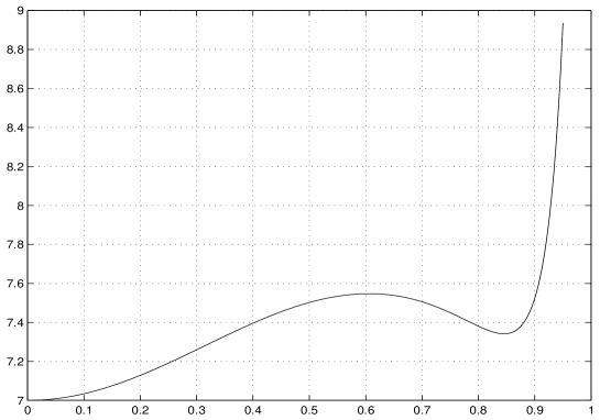
Figure 1: The energy of the giant graviton versus $r/R$ for fixed angular momentum. For the plot shown, $\tilde{\gamma}=0.4$, $N=10$ and ${\cal M}=7/N$. The energy is shown in units of $1/R$.

Clearly the energy of the point graviton is less than that of the giant, so that the giant graviton will be an unstable state. We will study the nature of this instability in the next section. The contributions to the Chern-Simons four form flux and $C_{2}\wedge B$ terms enter with opposite signs. At $\tilde{\gamma}=0$, the $C_{2}\wedge B$ term vanishes, while the four form flux term is non-zero. As $\tilde{\gamma}$ is increased, the $C_{2}\wedge B$ term grows faster than the four form flux term. For large enough deformations, the $C_{2}\wedge B$ term dominates. There is a critical deformation beyond which there is no giant graviton solution. This matches well with the study [30] of giants in a constant NSNS B field, in the maximally supersymmetric type IIB-plane wave background. Other work on non-spherical giants and giants in a $B$ field include[31].

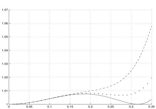
Figure 2: The energy of the giant graviton versus $r/R$ for fixed angular momentum. For the plot shown, $N=10$ and ${\cal M}=1/N$. The solid line has $\tilde{\gamma}=0$, the dotted line $\tilde{\gamma}=0.8$ and the dashed line $\tilde{\gamma}=1.6$. The energy is shown in units of $1/R$. As the deformation increases the giant graviton minimum is raised until it is no longer a solution.

3 Fluctuations

We have no guarantee that our ansatz of the previous section in fact minimizes the action. In this section we check that this is indeed the case and further, we study the spectrum of certain vibration modes of the giant. There are a number of interesting questions that can be answered using the vibration spectrum of giant gravitons. If our giants belong to a family of solutions that all have the same energy and angular momentum, there will be modes with zero energy. Secondly, if our giant graviton solution is (perturbatively) unstable, there will be tachyonic vibration mode(s). The excitations we consider correspond to motions of the branes in spacetime. Consequently, we do not consider the possibility of exciting fermionic modes or gauge fields that live on the giant graviton’s worldvolume. Our results show that the giant graviton is perturbatively stable. Finally, we argue that the giant graviton is corrected by quantum tunneling by constructing a bounce solution to the Euclidean equations of motion.

Our ansatz for the giant graviton is

$$\alpha_{i}=\epsilon\delta\alpha_{i},\qquad i=1,2,3,4,$$

$$\alpha=\alpha_{0}+\epsilon\delta\alpha,$$

$$\phi_{1}=\omega t+\epsilon\delta\phi_{1}.$$

$\alpha_{0}$ and $\omega$ are constants, independent of $y^{\mu}$. Despite their names, we have not yet given any reason to identify $\alpha_{0}$ and $\omega$ with the constants appearing in our ansatz of section 2. We now plug this ansatz into the action and expand in $\epsilon$. If the linear order in $\epsilon$ contribution to the action vanishes, for $\omega=\dot{\phi}_{1}$ computed using (1) and for the value of $\alpha_{0}$ that minimizes the energy, we know that the giants of section 2 minimize the action and that they are indeed classical solutions. The quadratic in $\epsilon$ contribution to the action can be used to learn about the energies of vibration modes of the giant.

Plugging this ansatz into the action and expanding, the term linear in $\epsilon$ is

$$\epsilon\int dy^{0}dy^{1}dy^{2}dy^{3}\left(A{\partial\delta\phi_{1}\over\partial t}+B\delta\alpha\right),$$

where

$$A = -{N\over 2\pi^{2}}\sin^{3}\alpha_{0}\sin y^{1}\cos y^{1}{\omega\cos^{2}\alpha_{0}\over\sqrt{1-\omega^{2}\cos^{2}\alpha}}-N\sin y^{1}\cos y^{1}{\tilde{\gamma}^{2}{r^{6}(R^{2}-r^{2})\over 2\pi^{2}R^{8}(1+\tilde{\gamma}^{2}{r^{2}\over R^{2}}(1-{r^{2}\over R^{2}}))}}$$

$$+ {2N\sin y^{1}\cos y^{1}\over\pi^{2}}\left[{\tilde{\gamma}-\sqrt{4+\tilde{\gamma}^{2}}\over 4\tilde{\gamma}^{2}\sqrt{4+\tilde{\gamma}^{2}}}\log\left({{2{r^{2}\over R^{2}}+{\sqrt{4+\tilde{\gamma}^{2}}\over\tilde{\gamma}}-1}\over{{\sqrt{4+\tilde{\gamma}^{2}}\over\tilde{\gamma}}-1}}\right)\right.$$

$$- \left.{{\tilde{\gamma}+\sqrt{4+\tilde{\gamma}^{2}}\over 4\tilde{\gamma}^{2}\sqrt{4+\tilde{\gamma}^{2}}}}\log\left({{-2{r^{2}\over R^{2}}+{\sqrt{4+\tilde{\gamma}^{2}}\over\tilde{\gamma}}+1}\over{{\sqrt{4+\tilde{\gamma}^{2}}\over\tilde{\gamma}}+1}}\right)\right],$$

$$B = {N\cos\alpha_{0}\sin^{2}\alpha_{0}\sin y^{1}\cos y^{1}\over 4\pi^{2}\sqrt{1-\omega^{2}\cos^{2}\alpha_{0}}}(6\omega^{2}\cos^{2}\alpha_{0}-2\omega^{2}\sin^{2}\alpha_{0}-6)+{2N\omega\cos\alpha_{0}\sin^{3}\alpha_{0}\sin y^{1}\cos y^{1}\over\pi^{2}(1+\tilde{\gamma}^{2}\cos^{2}\alpha_{0}\sin^{2}\alpha_{0})}$$

$$- {N\omega\tilde{\gamma}^{2}(3\sin^{5}\alpha_{0}\cos^{3}\alpha_{0}-\sin^{7}\alpha_{0}\cos\alpha_{0}+2\tilde{\gamma}^{2}\sin^{7}\alpha_{0}\cos^{5}\alpha_{0})\sin y^{1}\cos y^{1}\over\pi^{2}(1+\tilde{\gamma}^{2}\cos^{2}\alpha_{0}\sin^{2}\alpha_{0})^{2}}.$$

Now, notice that the coefficient $A$ is independent of time. This implies that the term in the first order change in the action involving $\delta\phi_{1}$ gives no contribution, because we vary with fixed boundary conditions, that is, $\delta\phi_{1}$ vanishes at the initial and final times. Using (1) and plotting $B$ as a function of $\alpha_{0}$, we find that the value of $\alpha_{0}$ that minimizes the energy is the same value of $\alpha_{0}$ that sets $B$ to zero.

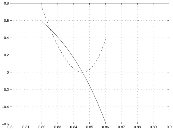
Figure 3: In the above plot $B$ is shown as the solid line; the energy of the giant graviton minus the minimum of the energy is shown as the dashed line. The $x$-axis is $r/R$. For the plot shown, $\tilde{\gamma}=0.4$, $N=10$ and ${\cal M}=7/N$. The energy is shown in units of $1/R$.

This confirms that the giant gravitons written down in section 2 are indeed solutions to the equations of motion following from the D3 brane action.

Expanding the action to second order in $\epsilon$ and varying with respect to $\delta\alpha_{i}$ we obtain the wave equation

$$\partial^{2}_{0}\delta\alpha_{i}+{1-\omega^{2}R^{2}\cos^{2}\alpha_{0}\over R^{2}\sin^{2}\alpha_{0}}L^{2}\delta\alpha_{i}-{\tilde{\gamma}^{2}\cos^{2}(\alpha_{0})\over R^{2}}(\partial_{2}-\partial_{3})^{2}\delta\alpha_{i}+{\delta\alpha_{i}\over R^{2}}=0,$$

where we have introduced the angular momentum squared $L^{2}$, which in our coordinates is given by

$$-{2\over\sin(2y^{1})}\left({1\over 2}\sin(2y^{1}){\partial\over\partial y^{1}}{\partial\over\partial y^{1}}+\cos(2y^{1}){\partial\over\partial y^{1}}+\tan y^{1}{\partial\over\partial y^{2}}{\partial\over\partial y^{2}}+\cot y^{1}{\partial\over\partial y^{3}}{\partial\over\partial y^{3}}\right).$$

The original $SO(4)$ worldvolume symmetry that we’d have in the undeformed case is broken to $U(1)\times U(1)$. These two $U(1)$ symmetries correspond to translations of $\phi_{2}$ and $\phi_{3}$. It is possible to choose spherical harmonics $Y^{l}_{m_{1},m_{2}}(y^{1},y^{2},y^{3})$ with definite $U(1)\times U(1)$ quantum numbers $(m_{1},m_{2})$. For spherical harmonics with $L^{2}=l(l+2)$ we have $|m_{1}|+|m_{2}|\leq l$. Making the ansatz

$$\delta\alpha_{i}=e^{iE^{l}_{m_{1},m_{2}}y^{0}}Y^{l}_{m_{1},m_{2}}(y^{1},y^{2},y^{3}),$$

we find

$$(E^{l}_{m_{1},m_{2}})^{2}={1\over R^{2}}+l(l+2)\left[{1-\omega^{2}R^{2}\cos^{2}\alpha_{0}\over R^{2}\sin^{2}\alpha_{0}}\right]+{\tilde{\gamma}^{2}\cos^{2}(\alpha_{0})\over R^{2}}(m_{1}-m_{2})^{2}.$$

Clearly these frequencies depend on $R\sin\alpha_{0}$, the radius of the giant. For a near maximal giant, we have $\sin\alpha_{0}\approx 1$ and $\cos\alpha_{0}\approx 0$, so that

$$(E^{l}_{m_{1},m_{2}})^{2}={1\over R^{2}}+{l(l+2)\over R^{2}}.$$

This is equal to the frequency obtained in [7] for giant gravitons in the undeformed AdS${}_{5}\times$S⁵ background. Note that this frequency is independent of the size of the graviton. This is true for all giant gravitons (not just the maximal giant) in the undeformed background[7].

Varying with respect to $\delta\phi_{1}$ and $\delta\alpha$ we obtain the following two (coupled) wave equations

$$\partial^{2}_{0}\delta\alpha+{1-\omega^{2}R^{2}\cos^{2}\alpha_{0}\over R^{2}\sin^{2}\alpha_{0}}L^{2}\delta\alpha-{\tilde{\gamma}^{2}\cos^{2}(\alpha_{0})\over R^{2}}(\partial_{2}-\partial_{3})^{2}\delta\alpha+A_{1}\delta\alpha+A_{2}\partial_{0}\delta\phi_{1}=0,$$

$$\partial^{2}_{0}\delta\phi_{1}+{1\over R^{2}\sin^{2}\alpha_{0}}L^{2}\delta\phi_{1}-{A_{2}\over\cos^{2}\alpha_{0}}\partial_{0}\delta\alpha=0,$$

where

$$A_{1}=-{2\left(6\omega^{2}\cos^{2}\alpha_{0}\cot^{2}\alpha_{0}-6\cot^{2}\alpha_{0}-10\omega^{2}\cos^{2}\alpha_{0}+3+\omega^{2}\sin^{2}\alpha_{0}+{\omega^{4}\sin^{2}\alpha_{0}\cos^{2}\alpha_{0}\over 1-\omega^{2}\cos^{2}\alpha_{0}}\right)\over\sqrt{1-\omega^{2}\cos^{2}\alpha_{0}}}$$

$$+{4\omega\tilde{\gamma}^{2}(15\sin\alpha_{0}\cos^{4}\alpha_{0}-16\sin^{3}\alpha_{0}\cos^{2}\alpha_{0}+\sin^{5}\alpha_{0}+14\tilde{\gamma}^{2}\sin^{3}\alpha_{0}\cos^{6}\alpha_{0}-10\tilde{\gamma}^{2}\sin^{5}\alpha_{0}\cos^{4}\alpha_{0})\over(1+\tilde{\gamma}^{2}\cos^{2}(\alpha_{0})\sin^{2}(\alpha_{0}))^{2}}$$

$$-{8\omega\tilde{\gamma}^{4}(3\sin^{3}\alpha_{0}\cos^{4}\alpha_{0}-\sin^{5}\alpha_{0}\cos^{2}\alpha_{0}+2\tilde{\gamma}^{2}\sin^{5}\alpha_{0}\cos^{6}\alpha_{0}(\cos^{2}\alpha_{0}-\sin^{2}\alpha_{0})\over(1+\tilde{\gamma}^{2}\cos^{2}(\alpha_{0})\sin^{2}(\alpha_{0}))^{3}}$$

$$-8\omega\left({3\cos\alpha_{0}\cot\alpha_{0}-\sin\alpha_{0}\over 1+\tilde{\gamma}^{2}\cos^{2}(\alpha_{0})\sin^{2}(\alpha_{0})}+{2\tilde{\gamma}^{2}\cos^{2}\alpha_{0}\sin\alpha_{0}(\sin^{2}\alpha_{0}-\cos^{2}\alpha_{0})\over(1+\tilde{\gamma}^{2}\cos^{2}(\alpha_{0})\sin^{2}(\alpha_{0}))^{2}}\right),$$

$$2A_{2} = {4\omega\cos\alpha_{0}-10\omega\cos^{3}\alpha_{0}\over\sin\alpha_{0}\sqrt{1-\omega^{2}\cos^{2}\alpha_{0}}}+{2\omega^{3}\cos^{3}\alpha_{0}\sin\alpha_{0}\over(1-\omega^{2}\cos^{2}\alpha_{0})^{3/2}}+4\omega\tilde{\gamma}^{2}{\sin^{2}\alpha_{0}\cos\alpha_{0}(\sin^{2}\alpha_{0}-\cos^{2}\alpha_{0})\over(1+\tilde{\gamma}^{2}\cos^{2}(\alpha_{0})\sin^{2}(\alpha_{0}))^{2}}$$

$$- {8\omega\tilde{\gamma}^{2}\cos^{3}\alpha_{0}\sin^{2}\alpha_{0}\over 1+\tilde{\gamma}^{2}\cos^{2}\alpha_{0}\sin^{2}\alpha_{0}}-{8\cos\alpha_{0}\over 1+\tilde{\gamma}^{2}\cos^{2}\alpha_{0}\sin^{2}\alpha_{0}}.$$

When $\tilde{\gamma}=0$, $\omega=1$ and

$$A_{1}=0,\qquad A_{2}=-{2\cos\alpha_{0}\over\sin^{2}\alpha_{0}}.$$

Using these values, it is easy to verify that we reproduce the undeformed results of [7]. Using the ansatz

$$\delta\alpha=A_{\alpha}e^{iE^{l}_{m_{1},m_{2}}y^{0}}Y^{l}_{m_{1},m_{2}}(y^{1},y^{2},y^{3}),\qquad\delta\phi_{1}=A_{\phi}e^{iE^{l}_{m_{1},m_{2}}y^{0}}Y^{l}_{m_{1},m_{2}}(y^{1},y^{2},y^{3}),$$

the energies of our fluctuations are found by solving

$${(E^{l}_{m_{1},m_{2}})^{4}\over\sin^{2}\alpha_{0}}+{l(l+2)\over R^{2}\sin^{2}\alpha_{0}}\left({A_{1}\over R^{2}}+\tilde{\gamma}^{2}(m-n)^{2}{\cos^{2}\alpha_{0}\over R^{2}}+{(1-\omega^{2}R^{2}\cos^{2}\alpha_{0})\over R^{2}\sin^{2}\alpha_{0}}l(l+2)\right)$$

$$-(E^{l}_{m_{1},m_{2}})^{2}\left({\tilde{\gamma}^{2}(m-n)^{2}\cos^{2}\alpha_{0}+A_{1}+l(l+2)(2-\omega^{2}R^{2}\cos^{2}\alpha_{0})\over R^{2}\sin^{2}\alpha_{0}}+{A_{2}^{2}(1-\omega^{2}R^{2}\cos^{2}\alpha_{0})\over R^{2}\cos^{2}\alpha_{0}}\right)=0.$$

We can now search for a perturbative instability, corresponding to an $E^{2}<0$ mode. The frequencies for the $\delta\alpha_{i}$ modes are manifestly positive. The analysis of the $\delta\phi_{1}$, $\delta\alpha$ coupled system is not as simple. In what follows, we will restrict ourselves to small deformations $\tilde{\gamma}\ll 1$. Obviously the positive energy modes can’t become unstable for small $\tilde{\gamma}$, so that we focus on the zero modes. The zero modes of the undeformed problem have $l=0$, so that we now focus on $l=0$. The $l=0$ modes satisfy

$$\partial^{2}_{0}\delta\alpha+A_{1}\delta\alpha+A_{2}\partial_{0}\delta\phi_{1}=0,$$

$$\partial^{2}_{0}\delta\phi_{1}-{A_{2}\over\cos^{2}\alpha_{0}}\partial_{0}\delta\alpha=0,$$

In the undeformed case, where $A_{1}$ is zero, there are two zero modes corresponding to constant shifts in $\phi_{1}$ and $\alpha$. In the deformed case, $A_{1}<0$ so that although there is still a zero mode associated with constant shifts of $\phi_{1}$, the zero mode associated with constant shifts of $\alpha$ is lifted.

Even though the giant is perturbatively stable, it may still be unstable due to tunneling effects. To investigate this possibility, we look for bounce solutions of the Euclidean equations of motion. In the underformed case, instantons linking the point graviton and sphere giants are known (see, for example, [32]). These solutions are obtained by allowing $\alpha$ (which determines the radius of the giant) to depend on time. Allowing both $\alpha$ and $\phi_{1}$ to depend on time, after integrating over the spatial worldvolume coordinates, we find the Lagrangian ($r$ is the radius of the giant)

$$L=-m\sqrt{1-a\dot{\phi}^{2}_{1}-\dot{\alpha}^{2}}+b\dot{\phi}_{1},$$

where

$$m=N{r^{3}\over R^{4}},\qquad a=R^{2}-r^{2},\qquad r=R\sin\alpha_{0}$$

$$b = 4N\left[{\tilde{\gamma}-\sqrt{4+\tilde{\gamma}^{2}}\over 4\tilde{\gamma}^{2}\sqrt{4+\tilde{\gamma}^{2}}}\log\left({{2{r^{2}\over R^{2}}+{\sqrt{4+\tilde{\gamma}^{2}}\over\tilde{\gamma}}-1}\over{{\sqrt{4+\tilde{\gamma}^{2}}\over\tilde{\gamma}}-1}}\right)-{{\tilde{\gamma}+\sqrt{4+\tilde{\gamma}^{2}}\over 4\tilde{\gamma}^{2}\sqrt{4+\tilde{\gamma}^{2}}}}\log\left({{-2{r^{2}\over R^{2}}+{\sqrt{4+\tilde{\gamma}^{2}}\over\tilde{\gamma}}+1}\over{{\sqrt{4+\tilde{\gamma}^{2}}\over\tilde{\gamma}}+1}}\right)\right]$$

$$- N{\tilde{\gamma}^{2}{r^{6}(R^{2}-r^{2})\over R^{8}(1+\tilde{\gamma}^{2}{r^{2}\over R^{2}}(1-{r^{2}\over R^{2}}))}.}$$

The canonical momenta are

$${\cal M}={\partial L\over\partial\dot{\phi}_{1}}={ma\dot{\phi}_{1}\over\sqrt{1-a\dot{\phi}^{2}_{1}-\dot{\alpha}^{2}}}+b,$$

$${\cal P}_{\alpha}={\partial L\over\partial\dot{\alpha}}={m\dot{\alpha}\over\sqrt{1-a\dot{\phi}^{2}_{1}-\dot{\alpha}^{2}}}.$$

The Hamiltonian is obtained, as usual, by performing a Legendre transformation. In what follows, we treat the momentum ${\cal M}$ as a constant and make the Euclidean continuations ${\cal P}_{\alpha}^{2}\to-{\cal P}_{\alpha}^{2}$ and $H\to-H$ to obtain

$$H=-\sqrt{m^{2}+{({\cal M}-b)^{2}\over a}-{\cal P}^{2}_{\alpha}}.$$

The Euclidean equations of motion are now

$$\dot{\alpha}={\partial H\over\partial{\cal P}_{\alpha}},\qquad\dot{\cal P}_{\alpha}=-{\partial H\over\partial\alpha}.$$

These equations of motion are solved by ${\cal P}_{\alpha}=0$ and $\alpha=\alpha_{0}$ a constant with $\sin\alpha_{0}$ the radius of the unstable giant. We have looked for numerical solutions to these equations by starting with ${\cal P}_{\alpha}=0$ and $\alpha=\alpha_{0}-\epsilon$ with $\epsilon\ll\alpha_{0}$. We find solutions as shown in figure 4 below.

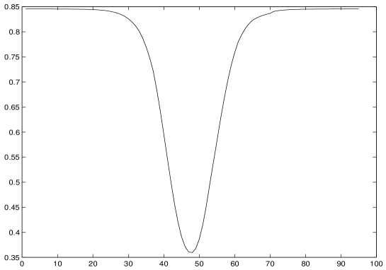
Figure 4: In the above plot $\alpha$ is shown as a function of $t$. The starting point is arbitrarily close to $\alpha_{0}$ where $\sin\alpha_{0}$ corresponds to the value of the radius of the giant graviton for $\tilde{\gamma}=0.4$, $N=10$ and ${\cal M}=7/N$.

Our solutions are periodic with the period becoming arbitrarily long as we decrease the value of $\epsilon$. The value of $\alpha$ decreases to a minimum before returning to its initial value. These bounce solutions signal that our giant is unstable due to tunneling effects[33].

4 Open Strings

The background studied in section 2 is conjectured[3] to be dual to the field theory with scalar potential

$$V=\mbox{Tr\,}\sum_{n>m=1}^{3}|e^{-i\pi\alpha_{mn}}\Phi_{m}\Phi_{n}-e^{i\pi\alpha_{mn}}\Phi_{n}\Phi_{m}|^{2}+\mbox{Tr\,}\sum_{n=1}^{3}\left[\Phi_{n},\bar{\Phi}_{n}\right]^{2},$$

where

$$\alpha_{mn}=-\epsilon_{mni}\gamma_{i}.$$

Below we will give a precise relation between the parameters $\gamma_{i}$ of the gauge theory and the parameters $\tilde{\gamma}_{i}$ of the gravity background. Our giant graviton solutions correspond to branes orbiting with angular momentum along the $\phi_{1}$ direction. The ${\cal R}$ charge of $\Phi_{1}$ corresponds to the angular momentum ${\cal M}$ of section 2. Thus, a giant graviton with angular momentum ${\cal M}$ should be dual to an operator built out of ${\cal M}N$ $\Phi_{1}$ fields. From now on we use $Z$ to denote $\Phi_{1}$ and $X,Y$ to denote $\Phi_{2},\Phi_{3}$. To match what was done in the dual gravitational theory we set $\gamma_{1}=0$ and $\gamma_{2}=\gamma_{3}=\gamma$ so that

$$V = \mbox{Tr\,}\left[|e^{i\pi\gamma}ZY-e^{-i\pi\gamma}YZ|^{2}+|e^{i\pi\gamma}XZ-e^{-i\pi\gamma}ZX|^{2}+|YX-XY|^{2}\right.$$

$$+ \left.\left[X,\bar{X}\right]^{2}+\left[Y,\bar{Y}\right]^{2}+\left[Z,\bar{Z}\right]^{2}\right].$$

We would like to determine the spin chain of this deformed ${\cal N}=4$ super Yang-Mills theory relevant for the dual description of open strings attached to giants. The spin chain for the deformed ${\cal N}=4$ super Yang-Mills theory was found in [34]; describing the open strings amounts to determining what boundary conditions must be imposed on this spin chain. In the undeformed theory with gauge group $U(N)$, operators dual to sphere giants are given by Schur polynomials of the totally antisymmetric representations[8], which are labeled by Young diagrams with a single column. The cut off on the number of rows of the Young diagram perfectly matches the cut off on angular momentum arising because the sphere giant fills the $S^{5}$ of the AdS${}_{5}\times$S⁵ geometry. For maximal giants, the Schur polynomials are determinant like operators. Attaching a string to the maximal giant gives an operator of the form

$${\cal O}=\epsilon^{j_{1}\cdots j_{N}}_{i_{1}\cdots i_{N}}Z^{i_{1}}_{j_{1}}\cdots Z^{i_{N-1}}_{j_{N-1}}(M_{1}M_{2}\cdots M_{n})^{i_{N}}_{j_{N}}.$$

The open string is given by the product $(M_{1}M_{2}\cdots M_{n})^{i_{N}}_{j_{N}}$. The $M_{i}$ could in principle be fermions, covariant derivatives of Higgs fields or Higgs fields themselves. To describe excitations of the string involving only coordinates from the $S^{5}$, we would restrict the $M_{i}$ to be Higgs fields. We will restrict ourselves even further and require that the $M_{i}$ are $Z$ or $Y$. A spin chain description can then be constructed by identifying $(M_{1}M_{2}\cdots M_{n})^{i_{N}}_{j_{N}}$ with a spin chain that has $n$-sites. If $M_{i}=Z$ the $i$th spin is spin up; if $M_{i}=Y$ the $i$th spin is spin down. It is not possible for $Z$’s to hop off and onto the string attached to a maximal giant; as soon as $M_{1}=Z$ or $M_{n}=Z$ the operator factorizes into a closed string plus a maximal giant graviton. This implies the boundary constraint $M_{1}\neq Z\neq M_{n}$. However, for non-maximal giants, $Z$’s can hop between the graviton and the open string. In this case, the number of sites in the spin chain is dynamical. If however, one identifies the spaces between the $Y$’s as lattice sites and the $Z$’s as bosons which occupy sites in this lattice, the number of sites is again conserved[19]. For the undeformed theory this leads to the Hamiltonian[19]

$$H=2\lambda\alpha^{2}+2\lambda\sum_{l=1}^{L}\hat{a}_{l}^{\dagger}\hat{a}_{l}-\lambda\sum_{l=1}^{L-1}\left(\hat{a}_{l}^{\dagger}\hat{a}_{l+1}+\hat{a}_{l}\hat{a}_{l+1}^{\dagger}\right)+\lambda\alpha(\hat{a}_{1}+\hat{a}_{1}^{\dagger})+\lambda\alpha(\hat{a}_{L}+\hat{a}_{L}^{\dagger}).$$

The operators in the above Hamiltonian are Cuntz oscillators[19]

$$a_{i}a_{i}^{\dagger}=I,\qquad a_{i}^{\dagger}a_{i}=I-|0\rangle\langle 0|.$$

For a giant with angular momentum $p/R$, the parameter

$$\alpha=\sqrt{1-{p\over N}},$$

measures how far from a maximal giant we are.

Due to the deformation, hopping is now accompanied by an extra phase. To see how this comes about, note that the deformation replaces

$$\left[Z,Y\right]\to ZYe^{i\pi\gamma}-YZe^{-i\pi\gamma},$$

$$\left[Z,Y\right]\left[Z,Y\right]^{\dagger}\to ZY\bar{Y}\bar{Z}+YZ\bar{Z}\bar{Y}-ZY\bar{Z}\bar{Y}e^{2\pi i\gamma}-YZ\bar{Y}\bar{Z}e^{-i2\pi\gamma}.$$

It is straight forward to see what interactions in the spin chain Hamiltonian these terms induce (the overbraces indicate Wick contractions)

$$\mbox{Tr\,}(YZ\overbrace{\bar{Z}\overbrace{\bar{Y})\mbox{Tr\,}(Y}Z}.....)\to\mbox{Tr\,}(YZ...)\leftrightarrow a_{l}^{\dagger}a_{l}$$

$$\mbox{Tr\,}(ZY\overbrace{\bar{Y}\overbrace{\bar{Z})\mbox{Tr\,}(Z}Y}...)\to\mbox{Tr\,}(ZY...)\leftrightarrow a_{l}^{\dagger}a_{l}$$

$$\mbox{Tr\,}(ZY\overbrace{\bar{Z}\overbrace{\bar{Y}e^{i2\pi\gamma})\mbox{Tr\,}(Y}Z}....)\to e^{i2\pi\gamma}\mbox{Tr\,}(ZY....)\leftrightarrow e^{i2\pi\gamma}a_{l}^{\dagger}a_{l+1}$$

$$\mbox{Tr\,}(YZ\overbrace{\bar{Y}\overbrace{\bar{Z}e^{-i2\pi\gamma})\mbox{Tr\,}(Z}Y}...)\to e^{-i2\pi\gamma}\mbox{Tr\,}(YZ...)\leftrightarrow e^{-i2\pi\gamma}a_{l}a_{l+1}^{\dagger}.$$

To hop onto the spin chain, we are hopping from the “zeroth site”, which is the Schur polynomial/giant graviton, and onto the first site of the string. The term which does this has an $e^{-i2\pi\gamma}$ coefficient. Another way to hop onto the spin chain is to hop from the $L+1$th site into the $L$th site. The term which does this has an $e^{i2\pi\gamma}$ coefficient. It is straight forward to argue for the phases when we hop off of the giant graviton. From the above discussion we see that the deformation modifies this Hamiltonian to

$$H = 2\lambda\alpha^{2}+2\lambda\sum_{l=1}^{L}\hat{a}_{l}^{\dagger}\hat{a}_{l}-\lambda\sum_{l=1}^{L-1}\left(\hat{a}_{l}^{\dagger}\hat{a}_{l+1}e^{i2\pi\gamma}+\hat{a}_{l}\hat{a}_{l+1}^{\dagger}e^{-i2\pi\gamma}\right)$$

$$+ \lambda\alpha(\hat{a}_{1}e^{i2\pi\gamma}+\hat{a}_{1}^{\dagger}e^{-i2\pi\gamma})+\lambda\alpha(\hat{a}_{L}e^{-i2\pi\gamma}+\hat{a}_{L}^{\dagger}e^{i2\pi\gamma}).$$

In the above derivation of the deformed Hamiltonian we have considered only the terms which look like $F$-terms. For this to be valid, it is necessary that the self energy, vector exchange and terms which look like $D$-terms, continue to cancel as they did in the supersymmetric theory. It has been argued[4] that this is indeed the case, using the similarity between the $\beta$ deformation[35] and non-commutative theories[36].

The semiclassical limit, in which the action derived from coherent states should provide a good approximation to the dynamics, is obtained by taking

$$L\sim\sqrt{N}\to\infty,\qquad\lambda\to\infty,$$

holding ${\lambda\over L^{2}}$, $L\gamma$ and $\alpha$ fixed. To obtain the low energy effective action, we will use the coherent states

$$|z\rangle=\sqrt{1-|z|^{2}}\sum_{n=0}^{\infty}z^{n}|n\rangle,$$

with parameter

$$z_{l}=r_{l}e^{i\phi_{l}},$$

for the $l$th site. The coherent state action is given as usual by

$$S=\int dt\left(i\langle Z|{\partial\over\partial t}|Z\rangle-\langle Z|H|Z\rangle\right).$$

In the above expression the coherent state $|Z\rangle$ is written as a product over all sites

$$|Z\rangle=\prod_{l}|z_{l}\rangle.$$

As an illustration of the manipulations which follow, we describe the evaluation of the first term in the action. It is straight forward to see that

$${\partial\over\partial t}|z_{l}\rangle=-{r_{l}\dot{r}_{l}\over\sqrt{1-r_{l}^{2}}}\sum_{n=0}^{\infty}r_{l}^{n}e^{in\phi_{l}}|n\rangle+\sqrt{1-r_{l}^{2}}\sum_{n=0}^{\infty}n\left({\dot{r}_{l}\over r_{l}}+i\dot{\phi}_{l}\right)r_{l}^{n}e^{in\phi_{l}}|n\rangle,$$

$$\langle z_{m}|{\partial\over\partial t}|z_{l}\rangle=i{r_{l}^{2}\dot{\phi}_{l}\over 1-r_{l}^{2}}\delta_{lm}.$$

Thus,

$$\langle Z|{\partial\over\partial t}|Z\rangle=i\sum_{l=1}^{L}{r_{l}^{2}\dot{\phi}_{l}\over 1-r_{l}^{2}}.$$

In the large $L$ limit, to leading order in $L$ we have

$$\langle Z|{\partial\over\partial t}|Z\rangle=iL\int_{0}^{1}{r(\sigma)^{2}\dot{\phi}(\sigma)\over 1-r(\sigma)^{2}}d\sigma.$$

A straight forward computation along these lines gives

$$S = -\int dt\left[L\int_{0}^{1}{r^{2}\dot{\phi}\over 1-r^{2}}d\sigma+2\lambda\alpha^{2}+{\lambda\over L}\int_{0}^{1}\left((r^{\prime})^{2}+r^{2}(\phi^{\prime}+2\pi\tilde{\gamma})^{2}\right)d\sigma\right.$$

$$+ \lambda\bar{z}(1)z(1)+\lambda\bar{z}(0)z(0)\left.+\lambda\alpha(z(0)+\bar{z}(0))+\lambda\alpha(z(1)+\bar{z}(1))\right].$$

We identify

$$\tilde{\gamma}=L\gamma.$$

Write this action in terms of $\gamma$ and rescale $\sigma\to{\sigma\over\pi}$. Clearly, the deformation replaces

$$\phi^{\prime}\to\phi^{\prime}+2L\gamma.$$

Lets now consider the description of the open strings using the dual sigma model. The undeformed case has been studied in[19]. The work [19] uses a coordinate system in which the brane is static, a gauge in which $p_{\phi_{2}}$ is homogeneously distributed along the string, $p_{\phi_{2}}=2{\cal J}$ and $\tau=t$. After taking a low energy limit, the string sigma model action is

$$-\sqrt{\lambda_{YM}}\int dt\int_{0}^{2\pi}{d\sigma\over 2\pi}\left[{r^{2}\dot{\phi}_{1}\over 1-r^{2}}+{\lambda_{YM}\over 8\pi^{2}{\cal J}^{2}}(r^{\prime 2}+r^{2}\phi_{1}^{\prime 2})\right],$$

in perfect agreement with the undeformed result from the field theory[19], after identifying $L={\cal J}$ and $\lambda_{YM}=8\pi^{2}\lambda$.

The background studied in section 2 can be obtained by performing a sequence of TsT transformations[3]. A TsT transformation exploits a two torus, with coordinates $(\phi_{1},\phi_{2})$ say, in the geometry. A TsT transformation begins with a $T$-duality with respect to $\phi_{1}$, then a shift $\phi_{2}\to\phi_{2}+\gamma\phi_{1}$ and finally a second $T$-duality along $\phi_{1}$. In the $AdS_{5}\times S^{5}$ background there are three natural tori $(\phi_{1},\phi_{2})$ $(\phi_{2},\phi_{3})$ and $(\phi_{3},\phi_{1})$. This allows three independent TsT transformations giving the three parameter deformation of section 2. See [3] for details. The TsT transformation has a particularly simple action on the string sigma model, something which was exploited in[3] to obtain the Lax pair for the bosonic part of the sigma model. To obtain the sigma model for the deformed theory, we simply need to shift[3]

$$\phi_{i}^{\prime}\to\phi_{i}^{\prime}-\epsilon_{ijk}\gamma_{j}p_{k}.$$

For the above action, we only need to consider $\phi_{1}^{\prime}$

$$\phi_{1}^{\prime}\to\phi_{1}^{\prime}-\epsilon_{1jk}\gamma_{j}p_{k}.$$

Next, since we set $X=0$ we know that $p_{3}=0$. Thus,

$$\phi_{1}^{\prime}\to\phi_{1}^{\prime}-\epsilon_{1j2}\gamma_{j}p_{2}=\phi_{1}^{\prime}-\epsilon_{132}\gamma_{3}p_{2}=\phi_{1}^{\prime}+\gamma_{3}p_{2}.$$

Now, we have set $\gamma_{3}=\gamma_{2}=\gamma$ and in our gauge $p_{2}=2{\cal J}$, so that

$$\phi_{1}^{\prime}\to\phi_{1}^{\prime}+2\gamma{\cal J}=\phi_{1}^{\prime}+2\gamma L.$$

This is in complete agreement with the spin chain result.

5 Summary

In this paper we have found giant graviton solutions in the deformed background with $\tilde{\gamma}_{1}=0$ and $\tilde{\gamma}_{2}=\tilde{\gamma}_{3}\equiv\tilde{\gamma}$. These giants have an energy which is greater than the energy of a point graviton. We have also considered the spectrum of small fluctuations about these giants. The spectrum depends on the radius of the giant in contrast to the undeformed case where the spectrum is independent of the size of the giant[7]. For small deformations, we have argued that the giant graviton is perturbatively stable. The Euclidean equations of motion admit a bounce solution indicating that the giant graviton will be unstable due to tunneling effects. We have also considered the semiclassical dynamics of open strings attached to these giants. We find that there is perfect quantitative agreement between the gauge theory and the string theory. Indeed, the deformation in the gauge theory exactly reproduces the TsT transformation relating the deformed and undeformed sigma models!

The comparison in this paper provides further quantitative agreement following from AdS/CFT duality in a non-supersymmetric case. Further, the fact that the giant graviton is unstable makes the quantitative agreement even more interesting.

There are a number of directions in which the present work can be extended. It would be interesting to look for giant gravitons in the general three parameter deformed background. One could also consider giants which have expanded into the AdS₅ space; the giant will be the same as the solution presented in[6]; the deformation should however modify the small fluctuation spectrum[7]. Further, the open string fluctuations we have considered are certainly not the most general fluctuations that can be considered. It would be interesting to extend our results to see if the agreement we have found continues to hold for more general open string configurations.

Acknowledgements: We would like to thank Rajsekhar Bhattacharyya and Jeff Murugan for pleasant discussions. This work is supported by NRF grant number Gun 2047219.

References

-
[1]
J. Maldacena, “The large N limit of superconformal field theories and supergravity,”
Adv. Theor. Math. Phys. 2 231 (1998), hep-th/9711200;
S. Gubser, I.R. Klebanov and A.M. Polyakov, “Gauge Theory Correlators from Non-critical String Theory,” Phys. Lett.B428 (1998) 105, hep-th/9802109;
E. Witten, “Anti-de Sitter Space and Holography,” Adv. Theor. Math. Phys. 2 (1998) 253, hep-th/9802150;
Ofer Aharony, Steven S. Gubser, Juan M. Maldacena, Hirosi Ooguri and Yaron Oz, “Large N Field Theories, String Theory and Gravity,” Phys. Rept. 323 (2000) 183, hep-th/9905111. - [2] O. Lunin and J.M. Maldacena, “Deforming Field Theories with global symmetry and their gravity duals,” hep-th/0502086.
- [3] S.A. Frolov, “Lax Pair for Strings in Lunin-Maldacena Background,” hep-th/0503201.
- [4] S.A. Frolov, R. Roiban and A.A. Tseytlin, “Gauge-string duality for (non)supersymmetric deformations of Super Yang-Mills Theory,” hep-th/0507021.
- [5] J. McGreevy, L. Susskind and N. Toumbas, “Invasion of the Giant Gravitons from Anti-de Sitter Space”, JHEP 0006 008 (2000), hep-th/0003075.
-
[6]
S. Das, A. Jevicki and S. Mathur, “Giant Gravitons, BPS Bounds and Noncommutativity,”
Phys. Rev. D63 044001 (2001), hep-th/0008088;
M.T. Grisaru, R.C. Myers and O. Tajford, “SUSY and Goliath,” hep-th/0008015, JHEP 0008 040 (2000);
A. Hashimoto, S. Hirano and N. Itzakhi, “Large Branes in AdS and their Field Theory Dual,” JHEP 0008 051 (2000), hep-th/0008016. -
[7]
S. Das, A. Jevicki and S. Mathur, “Vibration Modes of Giant Gravitons,”
Phys. Rev. D63 024013 (2001), hep-th/0009019;
-
[8]
S. Corley, A. Jevicki and S. Ramgoolam, “Exact Correlators of
Giant Gravitons from Dual SYM Theory”, Adv. Theor. Math.
Phys. 5, 809-839, 2002, hep-th/0111222;
V. Balasubramanian, M. Berkooz, A. Naqvi and M. Strassler, “Giant Gravitons in Conformal Field Theory”, JHEP 0204 (2002) 034, hep-th/0107119;
S. Corley and S. Ramgoolam, “Finite Factorization equations and sum rules for BPS Correlators in N=4 SYM Theory”, Nucl. Phys. B641, 131-187, 2002, hep-th/0205221. - [9] R. de Mello Koch and R. Gwyn, “Giant Graviton Correlators from Dual super Yang-Mills Theory,” JHEP 0411 081 (2004) hep-th/0410236.
-
[10]
A. Jevicki, “Non-perturbative Collective Field Theory,” Nucl. Phys.
B376 (1992) 75;
A. Jevicki and A. van Tonder, “Finite q-oscillator Description of 2D String Theory,” Mod. Phys. Lett. A11 (1996) 1397,hep-th/9601058;
A.P. Polychronakos, “Quasihole wavefunctions for the Calogero Model,” Mod. Phys. Lett. A11, (1996) 1273, cond-mat/9603132;
D. Berenstein, “A Toy Model for the AdS/CFT Correspondence,” hep-th/0403110. - [11] H. Lin, O. Lunin and J. Maldacena, “Bubbling AdS space and 1/2 BPS geometries,” hep-th/0409174.
- [12] A. Donos, A. Jevicki and J.P. Rodrigues, “Matrix Model Maps in AdS/CFT,” hep-th/0507124.
-
[13]
D. Berenstein, C.P. Hertzog and I.R. Klebanov, “Baryon Spectra and AdS/CFT Correspondence,”
JHEP 0206 047 (2002) hep-th/0202150;
O. Aharony, Y.E. Antebi, M. Berkooz and R. Fishman, “Holey sheets: Pfaffians and subdeterminants as D-brane operators in large gauge theories,” JHEP 0212 (2002) 069, hep-th/0211152;
D. Berenstein, “Shape and Holography: Studies of dual operators to giant gravitons,” Nucl. Phys. B675 (2003) 179, hep-th/0306090;
V. Balasubramanian, M.X. Huang, T.S. Levi and A. Naqvi, “Open Strings from super Yang-Mills”, JHEP 0208 (2002) 037,hep-th/0204196;
Vijay Balasubramanian, David Berenstein, Bo Feng, Min-xin Huang, “D-Branes in Yang-Mills Theory and Emergent Gauge Symmetry,” JHEP 0503 006, (2005), hep-th/0411205. - [14] David Berenstein, Samuel E. Vazquez, “Integrable Open Spin Chains from Giant Gravitons”, JHEP 0506 059, (2005), hep-th/0501078.
- [15] J.A. Minahan and K. Zarembo, “The Bethe-ansatz for super Yang-Mills,” JHEP 0303 013 (2003), hep-th/0212208.
-
[16]
N. Beisert, C. Kristhansen and M. Staudacher, “The Dilatation Operator of
conformal super Yang-Mills theory,” Nucl. Phys. B664, 131 (2003)
hep-th/0303060;
N. Beisert and M. Staudacher, “The SYM Integrable Super Spin Chain,” Nucl. Phys. B670, 439 (2003), hep-th/0307042;
N.Beisert, “The Dilatation Operator of Super Yang-Mills Theory and Integrability,” Phys. Rept. 405 1 (2005), hep-th/0407277. -
[17]
G. Mandal, N.V. Suryanarayana and S.R. Wadia, “Aspects of semiclassical strings in
AdS5,” Phys. Lett. B543 81 (2002), hep-th/0206103;
I. Bena, J. Polchinski and R. Roiban, “Hidden Symmetries of the AdSS5 Superstring,” Phys. Rev. D69 046002 (2004), hep-th/0305116;
B.C. Vallilo, “Flat Currents in Classical AdSS5 Pure Spinor Superstring,” JHEP 0403 037 (2004) hep-th/0307018. - [18] Niklas Beisert, “The Dynamic Spin Chain” Nucl. Phys. B682 487-520, (2004) hep-th/0310252.
- [19] David Berenstein, Diego H. Correa, Samuel E. Vazquez, “Quantizing Open Spin Chains with Variable Length: An Example from Giant Gravitons,” hep-th/0502172.
- [20] S.A. Frolov, R. Roiban and A.A. Tseytlin, “Gauge-string duality for superconformal deformations of Super Yang-Mills Theory,” hep-th/0503192.
- [21] N. Beisert and R. Roiban, “Beauty and the Twist: The Bethe Ansatz for Twisted SYM,” hep-th/0505187.
- [22] U. Gursoy and C. Nunez, “Dipole Deformations of N=1 SYM and Supergravity Backgrounds with Global Symmetry,” hep-th/0505100.
- [23] C. Ahn and J.F. Vazquez-Portiz, “Marginal Deformations with Global Symmetry,” hep-th/0505168.
- [24] J.P. Gauntlett, S. Lee, T Mateos and D. Waldram, “Marginal Deformations of Field Theories with AdS4 Duals,” hep-th/0505207.
- [25] D. Berenstein, J. M. Maldacena and H. Nastase, “Strings in flat space and pp waves from N = 4 super Yang Mills,” JHEP 0204, 013 (2002) hep-th/0202021.
-
[26]
V. Niarchos and N. Prezas, “BMN Operators for superconformal Yang-Mills
theories and associated string backgrounds,” JHEP 0306, 015 (2003),
hep-th 0212111;
R. de Mello Koch, J. Murugan, J. Smolic and M. Smolic, “Deformed PP-Waves from the Lunin-Maldacena Background,” hep-th/0505227;
T. Mateos, “Marginal Deformations of N=4 SYM and Penrose limits with Continuum Spectrum,” hep-th/0505243. -
[27]
A. Mauri, S. Penati, A. Santambrogio, D. Zanon,
“Exact Results in Planar N=1 Superconformal Yang-Mills Theory,” hep-th/0507282;
S. Penati, A. Santambrogio, D. Zanon, “Two-Point Correlators in the Beta-Deformed N=4 SYM at the next-to-leading Order,” hep-th/0506150;
D.Z. Freedman, Umut Gursoy, “Comments on the Beta-Deformed N=4 SYM Theory,” hep-th/0506128;
S.M. Kuzenko, A.A. Tseytlin, “Effective Action of Beta-Deformed N=4 SYM Theory and ADS/CFT,” hep-th/0508098. - [28] N.P. Bobev, H. Dimov, R.C. Rashkov, “Semiclassical Strings in Lunin-Maldacena Background,” hep-th/0506063.
- [29] Jorge G. Russo, “String Spectrum of Curved String Backgrounds Obtained by T-Duality and Shifts of Polar Angles,” hep-th/0508125.
- [30] S. Prokushkin and M. M. Sheikh-Jabbari, “Squashed giants: Bound states of giant gravitons,” JHEP 0407, 077 (2004) hep-th/0406053.
-
[31]
O. Lunin, S.D. Mathur, I.Y. Park and A. Saxena, “Tachyon condensation and ‘bounce’ in the D1-D5,”
Nucl. Phys. B679 299 (2004) hep-th/0304007;
J.M. Camino and A.V. Ramallo, “Giant gravitons with NSNS B field,” JHEO 0109 012 (2001) hep-th/0107142;
A. Mikhailov, “Giant gravitons from holomorphic,” JHEP 0011 027 (2000) hep-th/0010206;
A. Mikhailov, “Nonspherical giant gravitons and matrix theory,” hep-th/0208077;
D. Bak, “Supersymmetric branes in PP-wave background,” Phys. Rev. D67, 045017 (2003) hep-th/0204033. - [32] J. Lee, “Tunneling between the giant gravitons in AdS(5) x S(5),” Phys. Rev. D 64, 046012 (2001) hep-th/0010191.
-
[33]
S. R. Coleman,
Phys. Rev. D 15, 2929 (1977)
[Erratum-ibid. D 16, 1248 (1977)].
C. G. . Callan and S. R. Coleman, Phys. Rev. D 16, 1762 (1977). -
[34]
R. Roiban, “On Spin Chains and field theories,” JHEP 0409 023 (2004), hep-th/0312218;
D. Berenstein and S.A. Cherkis, “Deformations of N=4 SYM and integrable spin chain models,” Nucl. Phys. B702 49 (2004), hep-th/0405215. - [35] Robert G. Leigh, Matthew J. Strassler, “Exactly Marginal Operators and Duality in Four Dimensional N=1 Supersymmetric Gauge Theory,” Nucl. Phys. B447 95-136 (1995) hep-th/9503121 .
-
[36]
David Berenstein, Robert G. Leigh, “Discrete Torsion, AdS/CFT and Duality,” JHEP
0001 038 (2000), hep-th/0001055;
David Berenstein, Vishnu Jejjala, Robert G. Leigh, “Marginal and Relevant Deformations of N=4 Field Theories and Noncommutative Moduli spaces of Vacua,” Nucl.Phys. B589 196-248 (2000), hep-th/0005087. -
[37]
Martin Kruczenski, “Spin Chains and String Theory,” Phys. Rev. Lett. 93 161602, (2004),
hep-th/0311203;
M. Kruczenski, A.V. Ryzhov, A.A. Tseytlin, “Large Spin Limit of AdSS5 String Theory and Low-Energy Expansion of Ferromagnetic Spin Chains,” Nucl. Phys. B692 3-49, (2004), hep-th/0403120;
Gleb Arutyunov, Sergey Frolov, “Integrable Hamiltonian for Classical Strings on AdSS5,” JHEP 0502 059, (2005) hep-th/0411089.