Mirage Cosmology of $U(1)$ Gauge Field on Unstable D3 Brane Universe

Abstract

An unstable $D3$-brane universe governed by the DBI action of the tachyon field minimally coupled to a $U(1)$ gauge boson is examined. The cosmological evolution of this coupled system, is further analyzed, in terms of the expansion rate of the inflating brane, which is highly affected by the presence of the tachyonic and gauge field charges. We show, that the minimal coupling makes the effective brane density less divergent. However, for some sectors of the theory the tachyon is not able to regulate it in an efficient fashion. Also, a detailed analysis of the dependance of the effective brane density on the scale factor of the universe is performed, which leads to various cosmological models.

I Introduction

There has been remarkable progress since the seminal work of Guth Guth:1980zm which was one of the first works to incorporate particle physics in cosmological analyses. After the emergence of string theory, the missing link was to find a consistent way to accommodate stringy physics in cosmology. Among the series of models that attempted to fill this gap, brane gases emerged as a promising approach in terms of T-duality implemented in cosmology. Thus, in these models, one can study the case where our universe, is filled with a thermal bath of strings or even M-theory membranes such that the compact dimensions of the universe can be wrapped around branes. So in this fashion the winding numbers affect the cosmological evolution Alexander:2000xv ; Brandenberger:2001kj ; Brandenberger:1988aj ; Tseytlin:1991xk .

Quite recently Sen:2002nu ; Garousi:2000tr , it was shown that string theory can accommodate unstable Dp-brane configurations apart from the already known stable ones. Following along the same lines an effective action for non-BPS D-branes in Type II string theories was proposed, where the manifested instability is caused by the presence of the tachyon field. Roughly speaking, the action governing this system is still the Dirac-Born-Infeld action modified in a way, that after tachyon condensetation takes place we are left with stable D-branes. To this end, it is necessary, that one reverts to a decaying like tachyonic potential Kutasov:2000qp ; Kutasov:2004dj . Moreover, tachyon physics provided us with a deeper understanding regarding cosmological inflation Frolov:2002rr ; Kofman:2002rh ; Felder:2002sv ; Shiu:2002qe ; Gibbons:2002md ; Feinstein:2002aj ; Padmanabhan:2002sh ; Kim:2002zr ; Shiu:2002xp ; Gorini:2004by ; Piao:2003sc ; Panigrahi:2004qr . In the very elucidating review Gibbons:2003gb tachyon cosmology was also examined in terms of a ”No-Go theorem” of warped compactifications Gibbons:1984kp . For a more extensive analysis on this issue see Maldacena:2000yy and references therein.

However, several years ago, a different pathway was followed Randall:1999ee ; Randall:1999vf . Yet again, the inspiration came form $11$ -dim supergravity Horava:1996ma where instead of dealing with M-theory on $R^{10}\times{S^{1}/Z_{2}}$ the authors compactified a five dimensional AdS spacetime on $S^{1}/Z_{2}$. The salient trait of this model, was that our $4$ dimensional observed universe is fixed in one of the two hyperplanes of the orbifolded spacetime discribed above and that gravity is free to propagate in the bulk but the graviton is actually confined in our universe since its wave function decays exponentially as it tries to expand away from the visible brane. Of course, one can consider apart from warped compactification schemes as in RS model, the case of extra open dimensions ( addressing the hierarchy problem as well) as it is done in Arkani-Hamed:1998rs ; Antoniadis:1998ig . Also, a relevant extension (non-supersymmetric) based on the Intersecting Brane World scenarios has been found Cremades:2002dh .

If one seeks more concrete cosmological models in terms of D-brane physics, then it is useful to resort to brane world scenarios that are inspired from the well celebrated AdS/CFT correspondence Maldacena:1997re . An elegant cosmological construction based on this correspondence, was first introduced by Kehagias-Kiritsis Kehagias:1999vr and became known as mirage cosmology. In this context, we have the notion of a D$3$-brane representing our $4$-dim universe that is embedded in a higher dimensional ambient space filled with a stack of Dp-branes with p$>3$. The core of this approach, is based upon the fact, that the D$3$-brane probe follows a geodesic motion under the influence of the gravitational field generated by the stack of Dp-branes. It is also considered that the stack is much heavier than the probe so one can safely ignore the back-reaction. What is really interesting about this realization, is the fact that the motion of the D$3$-brane induces a cosmological evolution, even in the case where our universe is empty of matter. Therefore, any cosmological expansion or contraction of our visible universe can be attributed to energy density that can originate from anywhere else other than the probe brane such us the bulk. Due to the intrinsic richness of this model, a thorough analysis of its implications in various aspects of string and D-brane inspired cosmologies followed Papantonopoulos:2000xs ; Youm:2000mi ; Youm:2000ke ; Brax:2002qw ; Bozhilov:2002fa ; Kim:2002hk ; Piao:2002vf ; Boehm:2002kf ; Papantonopoulos:2004au ; Iwashita:2005wi .

One in principle, can also study mirage cosmology when considering tachyonic degrees of freedom living in the bulk Kim:2000ax ; Papantonopoulos:2000wv ; Diamandis:2002zn . While the basic aspects of these models will be discussed in the later part of this paper, it is worthwhile to mention, that other extensions can also be considered Jeong:2005py . In fact, our whole analysis is strongly influenced by this paper in which the tachyon field is constrained on the D$3$-brane probe. What we propose, is to examine the case where one also turns a gauge field on the brane which is minimally coupled to the tachyon. For completeness, we mention, that the study of winding tachyon coupled to a gauge field on null orbifolds can be found in Berkooz:2005ym .

The paper is organized as follows. In Section $2$, we introduce the fundamentals of our model while in Section $3$ we derive the equations of motion for both the tachyon and the gauge field dictated by a modified version of the DBI action for unstable Dp branes. In Section $3$, having the equations of motions at hand, we proceed by expressing the four dimensional induced metric on the brane in terms of the constant of motions of the system. The third section concludes, by setting forth the complete formulas for the induced effective action on the probe brane. Finally, in Section $4$, there is a discussion on the effects of the tachyon- gauge boson system on the cosmological expansion. We further analyze the effects of the tachyon on the energy density for an exponentially decaying tachyon potential trough a numerical integration of the equation of motions. Also, useful conclusions are drawn especially in reference to former works in this field.

II Geodesic Motion Of An Unstable D3-Brane

In this section, we are going to unfold the basic features of our proposed model while at the same time we will try to make contact with what has been done in related investigations. We start with the case of the gravitational background which is static in nature and spherically symmetric. The metric that describes it is given in the following general form

$$ds^{2}_{10}=g_{00}(r)dt^{2}+g(r)(d\overrightarrow{x})^{2}+g_{rr}dr^{2}+g_{S}(r)d\Omega_{5}$$ (1)

where the timelike part of the metric $g_{00}$ is negative.

We also consider a rolling complex tachyon solution of an unstable D$3$-brane minimally coupled to a massless gauge field

$$S_{3}=-T_{3}\int{d^{4}\xi}e^{-\phi}V(T)\sqrt{-det\tilde{K}_{\mu\nu}}-T_{3}\int{d^{4}\xi}\hat{C_{4}}$$ (2)

where

$$\tilde{K}_{\mu\nu}=K_{MN}\frac{\partial x^{M}}{\partial x^{\mu}}\frac{\partial x^{N}}{\partial x^{\nu}}$$ (3)

and

$$K_{MN}=g_{MN}+2\pi{\alpha}^{\prime}F_{MN}+\frac{1}{2}(D_{M}TD_{N}T^{*}+c.c)$$ (4)

We ascribe capital indices M,N for the bulk coordinates while $\mu,\nu$ are the one kept for the probe brane.

For completeness, we mention that $F_{\mu\nu}$ is the world volume antisymmetric gauge field strength and $G_{MN}$ is the induced metric on the D$3$-brane universe and $\phi$ is the dilaton. Note, that the RR field $\hat{C}(r)=C_{0...3}(r)$ is also included in the action. In addition, the form of the complex tachyon field and its covariant derivative are given as follows

$$D_{M}T=\partial_{M}T-iA_{M}T$$ (5)

$$T=T_{x}+iT_{y}$$ (6)

At this point, it is instructive to mention that our action which describes the tachyon minimally coupled to a $U(1)$ gauge field was initially proposed in a slightly different form in Sen:2003tm and implemented in a different context. In fact, the analysis of Barnaby:2004dp ; Cline:2005zy was mainly based upon investigating vortex like solutions when the tachyon field is coupled to two different gauge fields one originating from a D-brane and the other from a anti-brane. Therefore, the gauge group of the system is of the form $U(1)\times U(1)$. The basic principles of this model were also adopted in later works Barnaby:2004dp ; Cline:2005zy which were pertinent to cosmological backgrounds viewed in terms of brane-antibrane annihilation. In our action though, there is a single gauge field and we also have considered that the transverse scalar fields of the non-BPS brane are set to zero. Therefore, the tachyon potential has no dependence on these scalars but only on the tachyon field itself. Further, we demand that the tachyon is restricted on the moving brane so it depends exclusively on time.

Given the fact that our system respects reparametrization invariance, we are able to work on the static gauge, $x^{\alpha}=\xi^{\alpha},\alpha=0,1,2,3$. This particular choice of gauge will really simplify the calculations. Also, due to the angular part of the ambient space, the moving D$3$-brane does inherit a non zero angular momentum in the transverse dimensions. Having all of the above in mind the lagrangian is given by

$$L=-\sqrt{T^{2}_{3}V^{2}(T)e^{-2\phi}[g^{3}(r)(|g_{00}|-g^{rr}\dot{r}^{2}-g_{s}h_{ij}\dot{\varphi}^{i}\dot{\varphi}^{j}+\dot{T}^{2})-g^{2}(\alpha^{i}\dot{A}_{i}\dot{T}+\dot{A}_{i}\dot{A}^{i})]}+\hat{C}(r)$$ (7)

In order to bring the lagrangian in this form, we performed the following steps. First of all we considered without any loss of generality the following ansatz for the gauge field

$$A^{i}(t)=A^{i}_{0}+\tilde{A}^{i}(t)$$ (8)

where $A^{i}_{0}$ is independent of time

One can also view $\tilde{A}^{i}(t)$ as very small fluctuation of the gauge field around $A^{i}_{0}$. In other words, we assume, that our massless gauge field is very weak. With this assumption, only terms that are linear in the gauge field are considered while higher order terms are small and thus neglected. In addition to that, we are interested in solutions where the tachyon is really restrained to a region very close to the top of the tachyon potential which in general is taken to be of the following form

$$V(T)=\frac{V_{0}}{cosh(\frac{T}{T_{0}})}$$ (9)

At this point we note, that the potential which plays the role of a varying tension has the proper asymptotic behavior, meaning that $V(T=0)=1$ and $V(T=\infty)=0$. The significance of this approximation will be apparent later on. However, in our case the exact form of the tachyonic potential is not a crucial issue, since later on we work in a region where the potential is flat. Therefore under these two basic assumptions the form of Eq. (7) comes is natural. Further, in the rest of this paper the $2\pi\alpha^{\prime}$ factor is suppressed and for convenience we also drop the tilde from the gauge field. To further simplify our calculations we use the $A_{0}=0$ gauge. In addition, the imaginary part of the tachyon field is taken to be constant, i.e $T_{y}=c$. Therefore, one can naturally expresses the constants $\alpha^{i}$ as

$$\alpha^{i}=A^{i}_{0}c$$ (10)

where the index i runs over the three spatial dimensions.

With $T_{3}$ we denote the tension of the probe D$3$-brane, while the potential which drives the rolling tachyon is given by $V(T)$. As with the tachyon, the three dimensional induced components of the gauge field on the brane don’t depend on any other coordinates other than time.

We can also adopt the following redefinitions

$$M=T^{2}_{3}V^{2}(T)e^{-2\phi}g^{3}(r)|g_{00}|$$

$$B=T^{2}_{3}V^{2}(T)e^{-2\phi}g^{rr}(r)g^{3}(r)$$

$$C=T^{2}_{3}V^{2}(T)e^{-2\phi}g_{s}(r)g^{3}(r)$$

$$D=T^{2}_{3}V^{2}(T)e^{-2\phi}g^{3}(r)$$

$$E=T^{2}_{3}V^{2}(T)e^{-2\phi}g^{2}(r)$$

Thus the lagrangian is recast in the compact form

$$L=-\sqrt{M-B\dot{r}^{2}-Ch_{ij}\dot{\varphi}^{i}\dot{\varphi}^{j}-D\dot{T}^{2}-E(\alpha^{i}\dot{A}_{i}\dot{T}+\dot{A}_{i}\dot{A}^{i})}+\hat{C}(r)$$ (11)

III Classical Field Theory Equations Of Motion

In this section, since the general formalism of the paper is already illustrated, we provide the classical equation of motion for all fields in the Lagrangian through the variation principle.

The momenta are given by

$$P_{r}=\frac{B\dot{r}}{\sqrt{M-B\dot{r}^{2}-Ch_{ij}\dot{\varphi}^{i}\dot{\varphi}^{j}-D\dot{T}^{2}-E(\alpha^{i}\dot{A}_{i}\dot{T}+\dot{A}_{i}\dot{A}^{i})}}$$ (12)

$$P_{i}=\frac{Ch_{ij}\dot{\varphi}^{j}}{\sqrt{M-B\dot{r}^{2}-Ch_{ij}\dot{\varphi}^{i}\dot{\varphi}^{j}-D\dot{T}^{2}-E(\alpha^{i}\dot{A}_{i}\dot{T}+\dot{A}_{i}\dot{A}^{i})}}$$ (13)

In addition, the two dynamical fields (the tachyon and the gauge boson) of the system are also endowed with the following momenta

$$P_{T}=\frac{E\alpha^{i}\dot{A}_{i}+2D\dot{T}}{2\sqrt{M-B\dot{r}^{2}-Ch_{ij}\dot{\varphi}^{i}\dot{\varphi}^{j}-D\dot{T}^{2}-E(\alpha^{i}\dot{A}_{i}\dot{T}+\dot{A}_{i}\dot{A}^{i})}}$$ (14)

$$P_{\dot{A}_{i}}=\frac{E(\alpha^{i}\dot{T}+2\dot{A}^{i})}{2\sqrt{M-B\dot{r}^{2}-Ch_{ij}\dot{\varphi}^{i}\dot{\varphi}^{j}-D\dot{T}^{2}-E(\alpha^{i}\dot{A}_{i}\dot{T}+\dot{A}_{i}\dot{A}^{i})}}$$ (15)

Given the fact that the Lagrangian doesn’t exhibit any explicit dependance upon time, it is expected, that the energy is conserved. Therefore, the associated integral of motion is of the form

$$H=\mathcal{E}=\frac{M}{\sqrt{M-B\dot{r}^{2}-Ch_{ij}\dot{\varphi}^{i}\dot{\varphi}^{j}-D\dot{T}^{2}-E(\alpha^{i}\dot{A}_{i}\dot{T}+\dot{A}_{i}\dot{A}^{i})}}-\hat{C}(r)$$ (16)

We recall that since the ambient space is spherically symmetric, angular momentum must be conserved, namely, $h^{ij}\dot{\varphi}^{i}\dot{\varphi}^{j}=l^{2}$( as it will be shown shortly when examining closely the case of the near horizon limit of $AdS_{5}\times S^{5}$ black hole background). Thus,

$$h_{ij}\dot{\varphi}^{i}\dot{\varphi}^{j}=\frac{l^{2}}{C(C+l^{2})}(M-B\dot{r}^{2}-Ch_{ij}\dot{\varphi}^{i}\dot{\varphi}^{j}-D\dot{T}^{2}-E(\alpha^{i}\dot{A}_{i}\dot{T}+\dot{A}_{i}\dot{A}^{i}))$$ (17)

Next, we attempt to construct the equation of motion for the tachyon field. To this end, we write

$$\frac{\partial L}{\partial\dot{T}}=\frac{E\alpha^{i}\dot{A}_{i}+2D\dot{T}}{2\sqrt{M-B\dot{r}^{2}-Ch_{ij}\dot{\varphi}^{i}\dot{\varphi}^{j}-D\dot{T}^{2}-E(\alpha^{i}\dot{A}_{i}\dot{T}+\dot{A}_{i}\dot{A}^{i})}}$$ (18)

$$\frac{\partial L}{\partial T}=-\frac{dV}{dT}\sqrt{T^{2}_{3}e^{-2\phi}[g^{3}(r)(|g_{00}|-g^{rr}\dot{r}^{2}-g_{s}h_{ij}\dot{\varphi}^{i}\dot{\varphi}^{j}+\dot{T}^{2})-g^{2}(r)(\alpha^{i}\dot{A}_{i}\dot{T}+\dot{A}_{i}\dot{A}^{i})]}$$ (19)

From Eq. (19) we conclude, that if one knows the actual form of the potential which describes the motion of the rolling tachyon, then solving this equation can be accomplished in conjunction with the equation of motion of the gauge field. To make things simpler we resort to working in a regime where the tachyon rolls from the top of the potential where one can safely take $\frac{dV}{dT}\simeq 0$ Jeong:2005py .

Based upon this approximation one recovers the following integral of motion

$$\tilde{Q}=\frac{E\alpha^{i}\dot{A}_{i}+2D\dot{T}}{2\sqrt{M-B\dot{r}^{2}-Ch_{ij}\dot{\varphi}^{i}\dot{\varphi}^{j}-D\dot{T}^{2}-E(\alpha^{i}\dot{A}_{i}\dot{T}+\dot{A}_{i}\dot{A}^{i})}}$$ (20)

As far as the the $U(1)$ gauge field is concerned we set forth the following integrals of motion

$$Q_{i}=\frac{E(2\dot{A}_{i}+\alpha_{i}\dot{T})}{2\sqrt{M-B\dot{r}^{2}-Ch_{ij}\dot{\varphi}^{i}\dot{\varphi}^{j}-D\dot{T}^{2}-E(\alpha^{i}\dot{A}_{i}\dot{T}+\dot{A}_{i}\dot{A}^{i})}}$$ (21)

Henceforth, the RR term will not be explicitly written unless stated otherwise. We proceed by providing the set of equations for $(A_{i},T)$, the radial coordinate and the angular part of system as functions of $(M,B,C,D,E,\alpha^{i})$ and the constants $(l,\tilde{Q},Q_{i})$. After a laborious but straightforward calculation one gets

$$\dot{T}^{2}=(\frac{M}{\mathcal{E}}\frac{4\tilde{Q}-2\alpha^{i}Q_{i}}{4D-E\alpha^{i}\alpha_{i}})^{2}$$ (22)

$$(\dot{A}_{i})^{2}=(\frac{M}{2E\mathcal{E}}[2Q_{i}-(\frac{4\tilde{Q}-2\alpha^{j}Q_{j}}{4D-E\alpha^{j}\alpha_{j}})\alpha_{i}E])^{2}$$ (23)

$$h_{ij}\dot{\varphi}^{i}\dot{\varphi}^{j}=\frac{l^{2}}{C^{2}}\frac{M^{2}}{\mathcal{E}^{2}}$$ (24)

$$B\dot{r}^{2}=M-\frac{l^{2}}{C}\frac{M^{2}}{\mathcal{E}^{2}}-\frac{M^{2}}{\mathcal{E}^{2}}-\frac{M^{2}}{E\mathcal{E}^{2}}Q^{i}Q_{i}-\frac{M^{2}}{4\mathcal{E}^{2}}\frac{(4\tilde{Q}-2\alpha^{i}Q_{i})^{2}}{4D-E\alpha^{i}\alpha_{i}}$$ (25)

Last equation essentially tells us that the radial motion of the brane is accompanied by the constraint dictated by the positivity of its right hand side.

Before we conclude, it is worth mentioning that in the non relativistic limit the whole analysis can be well approximated through a more simplified version of Eq. (11). To be more precise, in the low energy regime the DBI action can be expanded in the following fashion

$$L=-\sqrt{M}-\frac{1}{2}\frac{B}{\sqrt{M}}\dot{r}^{2}-\frac{1}{2}\frac{C}{\sqrt{M}}h_{ij}\dot{\varphi}^{i}\dot{\varphi}^{j}-\frac{1}{2}\frac{D}{\sqrt{M}}\dot{T}^{2}-\frac{1}{2}\frac{E}{\sqrt{M}}(\alpha^{i}\dot{A}_{i}\dot{T}+\dot{A}_{i}\dot{A}^{i})+\hat{C}(r)$$ (26)

While this equation can safely describe the evolution of the probe universe in low energy scales (big scale factors), it fails to capture the underlying physics at very early times where the spatial dimensions are still very small. It is therefore very essential for our analysis not to expand the square root in the Lagrangian since we are mainly interested in calculating quantities like the effective energy density and pressure on the $D3$-brane as $a\rightarrow 0$.

A this point, the setup is ready to investigate the cosmological implications of the moving probe, which is going to be described in detail in the next section.

IV Cosmological Evolution of the D3-brane Probe

We are interested in giving a detailed account of the cosmological implications of the current model. Basically, what is needed is the exact form of the induced four dimensional metric on the D$3$-brane. That amounts to

$$d\hat{s}^{2}=(g_{00}+g_{rr}\dot{r}^{2}+g_{S}h_{ij}\dot{\varphi}^{i}\dot{\varphi}^{j})dt^{2}+d(\overrightarrow{x})^{2}$$ (27)

Therefore, by direct substitution of equations Eq. (24) and Eq. (25) into Eq. (27) the following form for the metric is recovered

$$d\hat{s}^{2}=-|g_{00}|^{2}(\frac{1}{\mathcal{E}^{2}}T^{2}_{3}V^{2}_{0}e^{-2\phi}g^{3}+\frac{1}{\mathcal{E}^{2}}Q_{i}Q_{i}+\frac{(2g\tilde{Q}-\alpha_{i}Q_{i})^{2}}{\mathcal{E}^{2}(4g^{2}-\alpha_{i}\alpha_{i})})dt^{2}+g(d\overrightarrow{x})^{2}$$ (28)

Close inspection reveals, that one can further simplify the above metric in a more compact form

$$d\hat{s}^{2}=-d\eta^{2}+g(r(\eta))(d\overrightarrow{x})^{2}$$ (29)

while the cosmic time is defined as

$$d\eta=\frac{|g_{00}|}{\mathcal{E}}\sqrt{T^{2}_{3}V^{2}_{0}e^{-2\phi}g^{3}+Q_{i}Q_{i}+\frac{(2g\tilde{Q}-\alpha_{i}Q_{i})^{2}}{(4g^{2}-\alpha_{i}\alpha_{i})}}dt$$ (30)

For completeness, we mention, that one can compute the apparent Ricci scalar curvature of the four dimensional D$3$ brane universe in terms of the induced effective energy density as follows

$$R_{4-d}=8\pi G(\rho_{eff}-3p_{eff})=8\pi G(4+a\frac{\partial}{\partial a})\rho_{eff}$$ (31)

Apparently, one infers, that the argument of the radical in Eq. (30) is not only non-positive but it is also singular as well when $4g^{2}(r)=\alpha_{i}\alpha_{i}$ unlike in models like Kehagias:1999vr . However, this is not that surprising because of the nontrivial nature of the gauge field-tachyon interaction. Nonetheless, we are mainly interested in the regime where the scale factor of the brane goes to zero. At that limit it is easy to check, that the argument in the radical is strictly nonnegative (for nonzero values of the $Q_{i}$ charges) while the singularity has been avoided.

We can also choose the scale factor of the universe to obey the relation $a^{2}=g$, as it is widely used in mirage cosmology. Therefore, the four-dimensional Friedman equation can be brought in the form

$$(\frac{\dot{a}}{a})^{2}=\frac{\mathcal{E}^{2}-(l^{2}g_{S}^{-1}+R^{2})|g_{00}|}{4g_{rr}|g_{00}|R^{2}}(\frac{g^{\prime}}{g})^{2}$$ (32)

where

$$R^{2}=T^{2}_{3}V^{2}_{0}e^{-2\phi}g^{3}+Q_{i}Q_{i}+\frac{(2g\tilde{Q}-\alpha_{i}Q_{i})^{2}}{(4g^{2}-\alpha_{i}\alpha_{i})}$$ (33)

The dot stands for differentiation with respect to cosmic time $\eta$, while the prime stands for derivatives with respect to the radial coordinate r. Also, the Hubble constant is defined as $H=\dot{a}/a$. On the other hand, Eq. (31) can also be viewed in terms of the effective matter density on the probe brane

$$\frac{8\pi G}{3}\rho_{eff}=\frac{\mathcal{E}^{2}-(l^{2}g_{S}^{-1}+R^{2})|g_{00}|}{4g_{rr}|g_{00}|R^{2}}(\frac{g^{\prime}}{g})^{2}$$ (34)

Interestingly enough, an observer residing on the moving D$3$-brane feels the cosmological evolution of the universe as a continuous change of the scale factor $a(\eta)$ which depends on the radial position r.

As an example, one can study the very characteristic example of the near-horizon limit of a black hole in an $AdS_{5}\times{S^{5}}$ spacetime. The linear element of this ambient space is

$$ds^{2}=\frac{r^{2}}{L^{2}}(-f(r)dt^{2}+(d\overrightarrow{x}^{2}))+\frac{L^{2}}{r^{2}}\frac{dr^{2}}{f(r)}+L^{2}d\Omega^{2}_{5}$$ (35)

where $f(r)=1-\frac{r_{0}^{4}}{r^{4}}$ and $\hat{C}(r)=\frac{r^{4}}{L^{4}}-\frac{r_{0}^{4}}{2L^{4}}$

In addition, the following identifications are made

$$g_{00}(r)=-\frac{r^{2}}{L^{2}}f(r)$$

$$g(r)=\frac{r^{2}}{L^{2}}$$

$$g_{rr}(r)=\frac{L^{2}}{r^{2}}\frac{1}{f(r)}$$

$$g_{S}(r)=L^{2}$$

which lead to the analogue of Friedman equation on the probe brane

$$H^{2}=\frac{8\pi G}{3}\rho_{eff}=\frac{1}{a^{2}L^{2}F^{2}}((\mathcal{E}+a^{4})^{2}-a^{2}(1-\frac{r_{0}^{4}}{L^{4}a^{4}})(F^{2}+\frac{l_{S}^{2}}{L^{2}}))$$ (36)

The constant term accompanying the RR term is absorbed in $\mathcal{E}$. The explicit form of F is given as a function of the scale factor of the universe in the following form

$$F^{2}=T^{2}_{3}V_{0}^{2}e^{-2\phi}a^{6}+Q_{i}Q_{i}+\frac{(2\tilde{Q}a^{2}-\alpha_{i}Q_{i})^{2}}{4a^{4}-\alpha_{i}\alpha_{i}}$$ (37)

Having laid out the basic constituents of our model, it is time to make some remarks with regarding its effects on cosmological evolution. Our results are in agreement with the vanishing gauge field case Jeong:2005py in which the effective density on the brane is given in the following form

$$\frac{8\pi G}{3}\rho_{eff}=\frac{1}{a^{2}(a^{6}e^{-2\phi}V_{0}^{2}T^{2}_{3}+Q^{2})L^{2}}[E^{2}-(1-\frac{r_{0}^{4}}{L^{4}}\frac{1}{a^{4}})a^{2}(a^{6}e^{-2\phi}V_{0}^{2}+Q^{2}+\frac{l^{2}}{L^{2}})]$$ (38)

After performing the following substitutions where, $Q\rightarrow{\tilde{Q}},E\rightarrow{\mathcal{E}}$, then it becomes apparent that equations Eq. (36) and Eq. (38) are identical in the case of vanishing Ramond-Ramond field. As it was also pointed out in Jeong:2005py the presence of the tachyonic charge $\tilde{Q}$, renders the effective brane density much less divergent than in Kehagias:1999vr , where $\rho_{eff}\sim a^{-8}$ as the scale factor approaches zero. One may also consider the case $l=r_{0}=0$. Here, the universe first expands when at some point in its history it stops and finally recollapses.

In a different limit where the tachyon field vanishes and the probe brane is stable ($V_{0}=1,\alpha_{i}=0,\tilde{Q}=0$), we were also able to reproduce equation (4.7) of Kehagias:1999vr after proper redefinition of variables. Another possible model is the one where both the gauge field and the tachyon are decoupled to each other ($\alpha_{i}=0$). Additionally, the positivity of the right hand side of Eq. (37) is restored and in general the complete form of the energy density reads as follows

$$\frac{8\pi G}{3}\rho_{eff}=\frac{1}{a^{2}(a^{6}e^{-2\phi}V_{0}^{2}T^{2}_{3}+\tilde{Q}^{2}+Q_{i}^{2})L^{2}}[(\mathcal{E}+a^{4})^{2}-(1-\frac{r_{0}^{4}}{L^{4}}\frac{1}{a^{4}})a^{2}(a^{6}e^{-2\phi}V_{0}^{2}+\tilde{Q}^{2}+Q_{i}^{2}+\frac{l^{2}}{L^{2}})]$$ (39)

where $Q_{i}^{2}=Q_{i}Q_{i}=|\overrightarrow{Q}|^{2}$.

Of course the most general model derived by our approach is the one dictated by Eq. (35). In particular, in the limit where $a\rightarrow 0$ one gets

$$F^{2}=T_{3}^{2}V_{0}e^{-2\phi}a^{6}+|\overrightarrow{Q}|^{2}sin^{2}{\theta}$$ (40)

where $\theta$ denotes the angle between vectors $\alpha_{i}$ and $Q_{i}$. In other words, the effective density is insensitive to the magnitude of $\alpha_{i}$ vector which in turn is proportional to the vacuum expectation value $A^{i}_{0}$ of the gauge boson Eq. (10). Note, that the singular behavior that the $F^{2}$ term exhibited in the most general case, has disappeared at the very early stages of the evolution of the universe. Further, equation Eq. (38) shows that there are sectors of the theory where $\rho_{eff}\sim a^{-8}$ when the cofactor of $|\overrightarrow{Q}|^{2}$ term is zero. To put it simply, in the case where a minimal coupling is included the effective density on the probe may have similar form with the one of a stable D3-brane universe. In all other cases this novel effect doesn’t occur due to the non vanishing charges. It is also apparent, that in Eq. (36) there is no explicit dependance on the tachyon charge and only the gauge field charges survives. This could be easily attributed to the well known fact that radiation dominates matter at early times in an expanding universe.

More precisely, in order that we acquire a more detailed picture of the properties of the cosmic fluid the exact form of the pressure needs to determined. The formula that associates the effective pressure with the density can be expressed in terms of the scale factor as follows

$$p_{eff}=-\rho_{eff}-\frac{1}{3}a\frac{\partial\rho_{eff}}{\partial{a}}$$ (41)

The last equation can be obtained through a direct implementation of Raychaudhuri equation which states as follows

$$\frac{\ddot{a}}{a}=(1+\frac{1}{2}a\frac{\partial}{\partial a})\frac{8\pi G}{3}\rho_{eff}=-\frac{4\pi G}{3}(\rho_{eff}+3p_{eff})$$ (42)

At the limit where the scale factor goes to zero the pressure reads

$$p_{eff}=\frac{1}{8\pi GL^{2}}\frac{r_{0}^{4}}{L^{4}}(1+\frac{l^{2}}{L^{2}}\frac{1}{Q_{i}^{2}sin^{2}{\theta}})\frac{1}{a^{4}}$$

$$+(\frac{\mathcal{E}^{2}}{8\pi GL^{2}})(-\frac{1}{(Q_{i}^{2}sin^{2}{\theta})^{2}}+\frac{8r_{0}^{4}}{L^{4}}\frac{l^{2}}{L^{2}}\frac{\alpha_{i}Q_{i}\tilde{Q}}{\alpha_{i}^{2}(Q_{i}^{2}sin^{2}{\theta})^{2}})\frac{1}{a^{2}}$$

$$+\frac{3}{8\pi GL^{2}}(1+\frac{l^{2}}{L^{2}}\frac{1}{Q_{i}^{2}sin^{2}{\theta}}+\frac{8\mathcal{E}^{2}}{3}\frac{\alpha_{i}Q_{i}\tilde{Q}}{\alpha_{i}^{2}(Q_{i}^{2}sin^{2}{\theta})^{2}}-\frac{16}{3}\frac{r_{0}^{4}}{L^{4}}\frac{l^{2}}{L^{2}}\frac{(\alpha_{i}Q_{i})^{2}}{\alpha_{i}^{4}})$$ (43)

while the effective density is of the form

$$\rho_{eff}=\frac{3}{8\pi GL^{2}}\frac{r_{0}}{L^{4}}(1+\frac{l^{2}}{L^{2}}\frac{1}{Q_{i}sin^{2}{\theta}})\frac{1}{a^{4}}+\frac{3\mathcal{E}^{2}}{8\pi GL^{2}}\frac{1}{(Q_{i}^{2}sin^{2}{\theta})^{2}}\frac{1}{a^{2}}-\frac{3}{8\pi GL^{2}}(1+\frac{l^{2}}{L^{2}}\frac{1}{Q_{i}^{2}sin^{2}{\theta}})$$ (44)

For an ideal fluid the state equation reads $p_{eff}=w\rho_{eff}$ so the constant $w$ encapsulates all the details of its structure. To be more precise, in the case where minimal coupling is included $w$ takes the following values $w=\frac{1}{3},-\frac{1}{3},-1$. Initially, the moving brane is radiation dominated but at later times it has the state equation of a universe filled with a cosmic fluid that resembles a nonzero cosmological constant. Thus, even though $w=-1$ the corresponding energy density is negative which is indicative of the unstable nature of the tachyon. For completeness we note that causality is respected at all times since the constraint $|w|\leq{1}$ is satisfied. The above values for $w$ are reminiscent of quintessence in which the accelerated expansion of the universe occurs when $-1<w<-\frac{1}{3}$. So for the probe brane, $w$ falls just outside of those bounds. A more extensive analysis on those limits with regard to the interplay between string theory and quintessential cosmological models can be found at Hellerman:2001yi ; Fischler:2001yj .

Finally one finds, that the term proportional to $a^{-2}$ in the energy density exhibits the same behavior as a negative curvature term which accelerates the expansion of the universe. In the most general case where the minimal coupling is taken into account, $w$ can take all shorts of values, however as long as we are looking back into the very early history of the expanding probe brane we observe that $p_{eff}=\frac{1}{3}\rho_{eff}$ holds. In addition, it is obvious that the inclusion of the minimal coupling will certainly give rise to regions where causality is violated, depending on the actual value of the free parameters of the theory which affect the state equation of the mirage mater. There is no doubt therefore, that the presence of the nontrivial coupling between the tachyon and the gauge field in the Lagrangian cannot drastically alter the state equation of the brane universe when the scale factor remains very small.

In has become more or less clear that our analysis focuses primarily on the effects of the kinetic term of the tachyon on the cosmological expansion rather than on it’s potential. However, a more detailed picture can be obtained by including the explicit form of the potential of the rolling tachyon. Even though it is really tough to get an analytic solution for the energy density we can still extract some useful information regarding the physics of our system through numerical analysis. To this end as well as to simplify things, we consider just the case where the tachyon lives on the brane in the absence of any fluxes. We further assume that the angular momentum $l$ is zero. By utilizing Eq. (13,14,16,18,19) which involve the equations of motions for the tachyon, the radial motion and the conservation of energy, one observes that the energy density is much less divergent as the scale factor goes to zero when tachyonic degrees of freedom are present on the brane. This is well transpired in our graph for a given set of initial conditions (see fig.1), while we also choose $T_{3}e^{-\phi}=1,\mathcal{E}=1,L=1$. In addition, the type of tachyon potential implemented in our analysis is exponentially decaying $V(T)\sim{e^{-T}}$ Sen:2002nu . Therefore, for appropriate initial conditions we reach the same conclusions as in the case where the tachyon is close to the top of the potential.

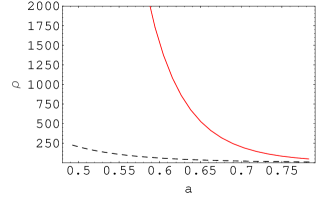
Figure 1: Plot of the effective brane density $\rho_{eff}$ as a function of the scale factor of the universe $a$. The red solid line represents the density when the tachyon is on the brane while the dark dashed line at the bottom shows the density when the tachyon is absent (stable D$3$-brane). The initial conditions used for both cases are $r=2,\frac{\partial{r}}{\partial{t}}=0.2,T=0,\frac{\partial{T}}{\partial{t}}=1.0$, regarding the radial and tachyonic equations of motions respectively at $t=0.1$.

V Conclusions

In this paper we have extended the mirage cosmological models to the case of tachyon matter living on the moving D$3$-brane which is coupled to $U(1)$ gauge field. Under the approximations that the gauge field is very weak and that the complex tachyon field is restrained on the top of the potential we derived the explicit form of the equations of motion for both dynamical fields. In fact, due to both the spherical symmetry of the $S^{5}$ part of the ambient space and energy conservation, the system is rendered integrable. Expressing the four dimensional induced metric in terms of the constants of motion enabled as to recast the metric in a form that describes a flat four dimensional universe. Eventually, the effective brane density was obtained giving rise to several cosmological interpretations. For instance, it was shown that the presence of the tachyon makes the cosmological expansion much less divergent at the early times of the evolution of the universe as it was pointed out in former works. The coupling between the two fields doesn’t alter this basic feature leading one to the conclusion that tachyon field acts like a regulator of the cosmological expansion in most cases. However, we did actually show, that in some regions of the theory the regulatory effect of the tachyon on the effective brane density is absent since it looks that the tachyon is unable to soften the degree of divergence that the effective energy density exhibits when the size of the universe is very small. Of course, in a more general treatment (which is out of the scope of this paper) where the gauge field becomes strong, one may lead to a different conclusion. Finally through a numerical analysis we show that even if one studies the motion of the tachyonic brane in the absence of gauge degrees of freedom the energy density is still softened for small scale factors given a decaying like tachyon potential. We hope, that future developments in this area will emerge, so that new aspects of tachyon cosmology will shed more light on the mechanisms affecting the very early stages of the universe.

Acknowledgements

The author would like to express his gratitude to Ioannis Bakas for his constant motivation, inspiration, support and for his comments on the manuscript. I would like to thank Elias Kiritsis for correspondence and suggestions, Pran Nath, Tomasz Taylor and Yogi Srivastava, for reading the paper and for their comments. Also, I thank Allan Widom for very useful and stimulating discussions and suggestions during the most crucial stages of this work. This work was supported in part by U.S. National Science Foundation grant NSF-PHY-$0546568$.

References

- (1) A. H. Guth, “The Inflationary Universe: A Possible Solution To The Horizon And Flatness Problems,” Phys. Rev. D 23, 347 (1981).
- (2) S. Alexander, R. H. Brandenberger and D. Easson, “Brane gases in the early universe,” Phys. Rev. D 62, 103509 (2000) [arXiv:hep-th/0005212].
- (3) R. Brandenberger, D. A. Easson and D. Kimberly, “Loitering phase in brane gas cosmology,” Nucl. Phys. B 623, 421 (2002) [arXiv:hep-th/0109165].
- (4) R. H. Brandenberger and C. Vafa, “Superstrings In The Early Universe,” Nucl. Phys. B 316, 391 (1989).
- (5) A. A. Tseytlin and C. Vafa, “Elements of string cosmology,” Nucl. Phys. B 372, 443 (1992) [arXiv:hep-th/9109048].
- (6) M. R. Garousi, Nucl. Phys. B 584, 284 (2000) [arXiv:hep-th/0003122]. E. A. Bergshoeff, M. de Roo, T. C. de Wit, E. Eyras and S. Panda, JHEP 0005, 009 (2000) [arXiv:hep-th/0003221]. A. Mazumdar, S. Panda and A. Perez-Lorenzana, Nucl. Phys. B 614, 101 (2001) [arXiv:hep-ph/0107058]. J. Kluson, Phys. Rev. D 62, 126003 (2000) [arXiv:hep-th/0004106]. D. Choudhury, D. Ghoshal, D. P. Jatkar and S. Panda, Phys. Lett. B 544, 231 (2002) [arXiv:hep-th/0204204].
- (7) A. Sen, “Rolling tachyon,” JHEP 0204, 048 (2002) [arXiv:hep-th/0203211]. A. Sen, “Tachyon matter,” JHEP 0207, 065 (2002) [arXiv:hep-th/0203265]. A. Sen, “Field theory of tachyon matter,” Mod. Phys. Lett. A 17, 1797 (2002) [arXiv:hep-th/0204143].
- (8) D. Kutasov, M. Marino and G. W. Moore, “Some exact results on tachyon condensation in string field theory,” JHEP 0010, 045 (2000) [arXiv:hep-th/0009148].
- (9) D. Kutasov, “D-brane dynamics near NS5-branes,” arXiv:hep-th/0405058.
- (10) A. V. Frolov, L. Kofman and A. A. Starobinsky, “Prospects and problems of tachyon matter cosmology,” Phys. Lett. B 545, 8 (2002) [arXiv:hep-th/0204187].
- (11) L. Kofman and A. Linde, “Problems with tachyon inflation,” JHEP 0207, 004 (2002) [arXiv:hep-th/0205121].
- (12) G. N. Felder, L. Kofman and A. Starobinsky, “Caustics in tachyon matter and other Born-Infeld scalars,” JHEP 0209, 026 (2002) [arXiv:hep-th/0208019].
- (13) G. Shiu and I. Wasserman, “Cosmological constraints on tachyon matter,” Phys. Lett. B 541, 6 (2002) [arXiv:hep-th/0205003].
- (14) G. W. Gibbons, “Cosmological evolution of the rolling tachyon,” Phys. Lett. B 537, 1 (2002) [arXiv:hep-th/0204008].
- (15) A. Feinstein, “Power-law inflation from the rolling tachyon,” Phys. Rev. D 66, 063511 (2002) [arXiv:hep-th/0204140].
- (16) T. Padmanabhan and T. R. Choudhury, “Can the clustered dark matter and the smooth dark energy arise from the same scalar field?,” Phys. Rev. D 66, 081301 (2002) [arXiv:hep-th/0205055].
- (17) C. j. Kim, H. B. Kim and Y. b. Kim, “Rolling tachyons in string cosmology,” Phys. Lett. B 552, 111 (2003) [arXiv:hep-th/0210101].
- (18) G. Shiu, S. H. H. Tye and I. Wasserman, “Rolling tachyon in brane world cosmology from superstring field theory,” Phys. Rev. D 67, 083517 (2003) [arXiv:hep-th/0207119].
- (19) V. Gorini, A. Kamenshchik, U. Moschella and V. Pasquier, “The Chaplygin gas as a model for dark energy,” arXiv:gr-qc/0403062.
- (20) Y. S. Piao and Y. Z. Zhang, “Thermal tachyon inflation,” arXiv:hep-th/0307074.
- (21) K. L. Panigrahi, Phys. Lett. B 601, 64 (2004) [arXiv:hep-th/0407134].
- (22) G. W. Gibbons, “Thoughts on tachyon cosmology,” Class. Quant. Grav. 20, S321 (2003) [arXiv:hep-th/0301117].
- (23) G. W. Gibbons, “Aspects Of Supergravity Theories,” Print-85-0061 (CAMBRIDGE) SPIRES entry Three lectures given at GIFT Seminar on Theoretical Physics, San Feliu de Guixols, Spain, Jun 4-11, 1984
- (24) J. M. Maldacena and C. Nunez, “Towards the large N limit of pure N = 1 super Yang Mills,” Phys. Rev. Lett. 86, 588 (2001) [arXiv:hep-th/0008001]. N. Ohta, “Accelerating cosmologies and inflation from M / superstring theories,” Int. J. Mod. Phys. A 20, 1 (2005) [arXiv:hep-th/0411230]. I. P. Neupane and D. L. Wiltshire, arXiv:hep-th/0504135.
- (25) L. Randall and R. Sundrum, “A large mass hierarchy from a small extra dimension,” Phys. Rev. Lett. 83, 3370 (1999) [arXiv:hep-ph/9905221].
- (26) L. Randall and R. Sundrum, “An alternative to compactification,” Phys. Rev. Lett. 83, 4690 (1999) [arXiv:hep-th/9906064].
- (27) P. Horava and E. Witten, “Eleven-Dimensional Supergravity on a Manifold with Boundary,” Nucl. Phys. B 475, 94 (1996) [arXiv:hep-th/9603142].
- (28) N. Arkani-Hamed, S. Dimopoulos and G. R. Dvali, “The hierarchy problem and new dimensions at a millimeter,” Phys. Lett. B 429, 263 (1998) [arXiv:hep-ph/9803315].
- (29) I. Antoniadis, N. Arkani-Hamed, S. Dimopoulos and G. R. Dvali, “New dimensions at a millimeter to a Fermi and superstrings at a TeV,” Phys. Lett. B 436, 257 (1998) [arXiv:hep-ph/9804398].
- (30) D. Cremades, L. E. Ibanez and F. Marchesano, Nucl. Phys. B 643, 93 (2002) [arXiv:hep-th/0205074]. C. Kokorelis, Nucl. Phys. B 677, 115 (2004) [arXiv:hep-th/0207234].
- (31) J. M. Maldacena, “The large N limit of superconformal field theories and supergravity,” Adv. Theor. Math. Phys. 2, 231 (1998) [Int. J. Theor. Phys. 38, 1113 (1999)] [arXiv:hep-th/9711200].
- (32) A. Kehagias and E. Kiritsis, “Mirage cosmology,” JHEP 9911, 022 (1999) [arXiv:hep-th/9910174].
- (33) E. Papantonopoulos, “Brane inflation from mirage cosmology,” arXiv:hep-th/0011051.
- (34) D. Youm, “Brane inflation in the background of D-brane with NS B field,” Phys. Rev. D 63, 125019 (2001) [arXiv:hep-th/0011024].
- (35) D. Youm, “Closed universe in mirage cosmology,” Phys. Rev. D 63, 085010 (2001) [Erratum-ibid. D 63, 129902 (2001)] [arXiv:hep-th/0011290].
- (36) P. Brax and D. A. Steer, “Non-BPS brane cosmology,” JHEP 0205, 016 (2002) [arXiv:hep-th/0204120].
- (37) P. Bozhilov, “Probe branes dynamics in nonconstant background fields,” arXiv:hep-th/0206253.
- (38) J. Y. Kim, “Mirage cosmology in M-theory,” Phys. Lett. B 548, 1 (2002) [arXiv:hep-th/0203084].
- (39) Y. S. Piao, R. G. Cai, X. m. Zhang and Y. Z. Zhang, Phys. Rev. D 66, 121301 (2002) [arXiv:hep-ph/0207143].
- (40) T. Boehm and D. A. Steer, “Perturbations on a moving D3-brane and mirage cosmology,” Phys. Rev. D 66, 063510 (2002) [arXiv:hep-th/0206147].
- (41) E. Papantonopoulos and V. Zamarias, “AdS/CFT correspondence and the reheating of the brane-universe,” JHEP 0410, 051 (2004) [arXiv:hep-th/0408227].
- (42) Y. Iwashita, T. Shiromizu, K. Takahashi and S. Fujii, Phys. Rev. D 71, 083518 (2005) [arXiv:hep-th/0503036].
- (43) J. Y. Kim, “Brane inflation in tachyonic and non-tachyonic type 0B string theories,” Phys. Rev. D 63, 045014 (2001) [arXiv:hep-th/0009175].
- (44) E. Papantonopoulos and I. Pappa, “Cosmological evolution of a brane universe in a type 0 string Phys. Rev. D 63, 103506 (2001) [arXiv:hep-th/0010014].
- (45) G. A. Diamandis, B. C. Georgalas, N. E. Mavromatos and E. Papantonopoulos, “Acceleration of the universe in type-0 non-critical strings,” Int. J. Mod. Phys. A 17, 4567 (2002) [arXiv:hep-th/0203241].
- (46) D. H. Jeong and J. Y. Kim, “Mirage cosmology with an unstable probe D3-brane,” Phys. Rev. D 72, 087503 (2005) [arXiv:hep-th/0502130].
- (47) M. Berkooz, Z. Komargodski, D. Reichmann and V. Shpitalnik, arXiv:hep-th/0507067.
- (48) A. Sen, “Dirac-Born-Infeld action on the tachyon kink and vortex,” Phys. Rev. D 68, 066008 (2003) [arXiv:hep-th/0303057].
- (49) N. Barnaby and J. M. Cline, “Creating the universe from brane-antibrane annihilation,” Phys. Rev. D 70, 023506 (2004) [arXiv:hep-th/0403223].
- (50) J. M. Cline, “Inflation from string theory,” arXiv:hep-th/0501179.
- (51) S. Hellerman, N. Kaloper and L. Susskind, “String theory and quintessence,” JHEP 0106, 003 (2001) [arXiv:hep-th/0104180].
- (52) W. Fischler, A. Kashani-Poor, R. McNees and S. Paban, “The acceleration of the universe, a challenge for string theory,” JHEP 0107, 003 (2001) [arXiv:hep-th/0104181].