Introduction and Summary

The domain wall is one of the important solitons in many areas of physics, such as particle physics, cosmology and condensed matter physics. Recently, the 1/2 BPS domain walls in the ${\cal N}=2$ supersymmetric (SUSY) non-Abelian $U(N_{\rm C})$ gauge theories were intensively studied and their moduli space was found to be the complex Grassmann manifold [1, 2]. When several non-parallel 1/2 BPS domain walls coexist, a 1/4 of SUSY is preserved by the configuration, which is called a 1/4 BPS state [3]. In the previous paper [4] we have found that multiple walls in the Abelian-Higgs system develop a web as a 1/4 BPS state similarly to $(p,q)$-string/5-brane webs in superstring theory. The junction charge, called the $Y$-charge, has been found to be always negative in the Abelian gauge theory [4, 5] as well as in generalized Wess-Zumino models [6], which can be understood as binding energy of the constituent domain walls. We also have found that the total moduli space of the webs, defined by all topological sectors patched together, to be the complex Grassmann manifold for the $U(N_{\rm C})$ gauge theory.

The purpose of this paper is to study 1/4 BPS webs of walls in the non-Abelian gauge theories by extending the previous analysis [4] to the ${\cal N}=2$ SUSY $U(N_{\rm C})$ gauge theories coupled with $N_{\rm F}(>N_{\rm C})$ Higgs fields (hypermultiplets) in the fundamental representation. There exist two kinds of nontrivial domain wall junctions. One is the Abelian junction characterized by a negative $Y$-charge. The other is the non-Abelian junction with a positive $Y$-charge. We find that opposite sign of the $Y$-charge can be attributed to quite a different internal structures of the Abelian and non-Abelian junctions. The non-Abelian $Y$-charge can be identified with the charge of the Hitchin system [7] which is positive. Besides these two kinds of junctions, there exist trivial intersections of penetrable walls [1] with vanishing $Y$-charge. Generally, walls in the non-Abelian gauge theories constitute very rich variety of webs of the Abelian and non-Abelian junctions and the intersections of penetrable walls. We find rules of the construction of the webs. Qualitative properties of the webs can be easily understood in terms of the grid diagram capturing the most relevant informations of the complex Grassmann manifold. On the other hand, their quantitative properties are clarified by moduli parameters corresponding to web configurations. Especially, difference between the Abelian junctions and the non-Abelian junctions can be understood by an embedding relation of the complex Grassmann manifold into a complex projective space which is called Plücker embedding. We explicitly identify normalizable modes of the webs with loops, which gives a $1+1$ dimensional ${\cal N}=(2,0)$ SUSY sigma model as the effective theory on the web.

This paper is organized by two parts. We devote the first part to clarify the qualitative properties of the webs. In the second part we concentrate on their quantitative properties.

Webs of walls in the SUSY Yang-Mills theory

Let us start with the 1+3 dimensional ${\cal N}=2$ SUSY $U(N_{\rm C})$ gauge theory coupled to the $N_{\rm F}(>N_{\rm C})$ hypermultiplets in the fundamental representation. The physical bosonic fields are a gauge field $W_{\mu}$ and a complex scalar $\Sigma=\Sigma_{1}+i\Sigma_{2}$, in the vector multiplet and complex scalars $H^{irA}$ $(r=1,2,\cdots,N_{\rm C},\ A=1,2,\cdots,N_{\rm F},\ i=1,2)$ in the hypermultiplets. We turn on completely non-degenerate complex masses for the hypermultiplets, which can be expressed as a diagonal mass matrix $M={\rm diag}(\mu_{1},\cdots,\mu_{N_{\rm F}})$ with $\mu_{A}\in{\bf C}$. In the following we will use both the complex notation $\mu_{A}=m_{A}+in_{A}\ (M=M_{1}+iM_{2})$ and the two-vector notation $\vec{\mu}_{A}=(m_{A},n_{A})$ for masses. We also turn on the Fayet-Iliopoulos (FI) parameter $c>0$ in the third direction of $SU(2)_{R}$ triplet. We consider minimal kinetic terms for all the fields. The scalar potential is

$$V={\rm Tr}\left[\frac{1}{g^{2}}\sum_{a=1}^{3}\left(Y^{a}\right)^{2}+\sum_{\alpha=1}^{2}\left(H^{i}M_{\alpha}-\Sigma_{\alpha}H^{i}\right)\left(H^{i}M_{\alpha}-\Sigma_{\alpha}H^{i}\right)^{\dagger}-\frac{1}{g^{2}}\left[\Sigma_{1},\Sigma_{2}\right]^{2}\right],$$ (1)

with $Y^{a}\equiv\frac{g^{2}}{2}\left(c^{a}{\bf 1}_{N_{\rm C}}-(\sigma^{a})^{j}{{}_{i}}H^{i}(H^{j})^{\dagger}\right)$. There exist ${}_{N_{\rm F}}C_{N_{\rm C}}=N_{\rm F}!/N_{\rm C}!(N_{\rm F}-N_{\rm C})!$ discrete vacua where gauge symmetry is fully broken [8]. Each vacuum is characterized by a set of $N_{\rm C}$ different flavor indices $\langle A_{1}A_{2}\cdots A_{N_{\rm C}}\rangle$ out of $N_{\rm F}$ flavors. In the rest of this article we may use a notation $\langle A_{r}\rangle$ short for $\langle A_{1}A_{2}\cdots A_{N_{\rm C}}\rangle$. In the vacuum $\langle A_{r}\rangle$, the vacuum expectation values (VEVs) of the hypermultiplets are $H^{1rA}=\sqrt{c}\delta^{A_{r}}{{}_{A}},\ H^{2rA}=0$ and the VEV of the adjoint scalar is $\Sigma={\rm diag}(\mu_{A_{1}},\cdots,\mu_{A_{N_{\rm C}}}).$ We express $N_{\rm C}\times N_{\rm F}$ matrix of the hypermultiplets by $H^{i}$ and set $H^{2}=0$ with $H\equiv H^{1}$ when we consider domain wall solutions in the following.

Single 1/2 BPS walls interpolate between two vacua $\left<\ \underline{\cdots}\ A\right>$ and $\left<\ \underline{\cdots}\ B\right>$ with only one different label. Here the underlines denote the same set of integers (ordering of integers does not affect anything). These walls are characterized by a complex central charge in the SUSY algebra

$$Z=c(\mu_{A}-\mu_{B})=c\left[(m_{A}-m_{B})+i(n_{A}-n_{B})\right].$$ (2)

By reexpressing this charge as $Z=Te^{i\theta}$, we can read the tension $T$ and the angle $\theta$ of normal vector $\vec{n}_{\theta}=(\cos\theta,\sin\theta)$ to the wall in the spatial $x^{1}$-$x^{2}$ plane.

Domain walls in the Abelian gauge theory were known to have the following internal structures [9]. There are two cases according to the value of the dimensionless parameter $g\sqrt{c}/|\Delta m+i\Delta n|$. Walls have a three-layer structure shown in Fig. 1(a), in the case of $g\sqrt{c}\ll|\Delta m+i\Delta n|$ (at weak gauge coupling). The outer two thin layers have the same width of order $L_{\rm o}=1/g\sqrt{c}$ and the internal fat layer has width of order $L_{\rm i}=|\Delta m+i\Delta n|/g^{2}c$. In the Fig. 1(a) the wall interpolates between the vacuum $\langle 1\rangle\ \left(H=\sqrt{c}(1,0),\ \Sigma=m_{1}\right)$ at $x^{1}\to-\infty$ and the vacuum $\langle 2\rangle\ \left(H=\sqrt{c}(0,1),\ \Sigma=m_{2}\right)$ at $x^{1}\to+\infty$. The first (second) flavor component of the Higgs field exponentially decreases in the left (right) outer layer so that the entire $U(1)$ gauge symmetry is restored in the inner core.

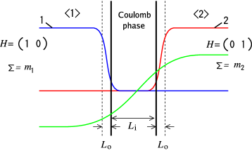
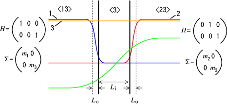
(a) Abelian gauge theory		(b) non-Abelian gauge theory

Figure 1: Internal structures of the domain walls with $g\sqrt{c}\ll|\Delta m+i\Delta n|$.

On the other hand, in the case of the walls in the non-Abelian gauge theories, the internal structure is a little bit different from that in the Abelian gauge theory. For simplicity, let us explain it in the $U(2)$ gauge theory with three flavors. A wall interpolating between the vacuum $\langle 13\rangle\ \big{(}H=\sqrt{c}\left(\begin{smallmatrix}1&0&0\\ 0&0&1\end{smallmatrix}\right),\ \Sigma=\left(\begin{smallmatrix}m_{1}&0\\ 0&m_{3}\end{smallmatrix}\right)\big{)}$ at $x^{1}\to-\infty$ and the vacuum $\langle 23\rangle\ \big{(}H=\sqrt{c}\left(\begin{smallmatrix}0&1&0\\ 0&0&1\end{smallmatrix}\right),\ \Sigma=\left(\begin{smallmatrix}m_{2}&0\\ 0&m_{3}\end{smallmatrix}\right)\big{)}$ at $x^{1}\to+\infty$ has the three-layer structure in the limit $g\sqrt{c}\ll|\Delta m+i\Delta n|$ (at weak gauge coupling). The first and the second components of the Higgs fields exponentially decrease in the two outer layers and almost vanish in the middle layer, whereas the third flavor component gets non-vanishing values over the whole region. Hence only the Abelian subgroup acting on the first color component is recovered in the middle layer of the wall, while the overall $U(1)$ is broken. We denote this phase in the middle layer by the flavor with a constant VEV like $\langle 3\rangle$ as shown in Fig. 1(b). In the opposite limit $g\sqrt{c}\gg|\Delta m+i\Delta n|$ (at strong gauge coupling), the internal structure becomes simpler for both Abelian and non-Abelian cases. There the middle layer disappears while two outer layers of the Higgs phase grow. The width of the wall is of order $1/|\Delta m+i\Delta n|$.

A web of walls contains several constituent walls with different slopes in the $x^{1}$-$x^{2}$ space. Each of them preserves different 1/2 SUSY and their webs preserve the 1/4 SUSY. The corresponding 1/4 BPS equations for the webs of walls are obtained [4] as

$$\left[\mathcal{D}_{1}+\Sigma_{1},\mathcal{D}_{2}+\Sigma_{2}\right]=0,\quad\mathcal{D}_{\alpha}H=HM_{\alpha}-\Sigma_{\alpha}H,\quad\sum_{\alpha}\mathcal{D}_{\alpha}\Sigma_{\alpha}=\frac{g^{2}}{2}\left(c{\bf 1}_{N_{\rm C}}-HH^{\dagger}\right),$$ (3)

with $\alpha=1,2$. The 1/4 BPS condition assures the equilibrium for tensions of walls, and the conservation of central charges ($\sum_{l}Z_{l}=0$) at every junction point. Here index $l$ labels the walls extending from that junction point. Configurations of wall junctions are characterized by another central charge ($Y$-charge) in the SUSY algebra

$$Y=-\frac{2}{g^{2}}\int dx^{1}dx^{2}\ \partial_{\alpha}{\rm Tr}\left(\epsilon^{\alpha\beta}\Sigma_{1}\mathcal{D}_{\beta}\Sigma_{2}\right).$$ (4)

In our theory elementary wall junctions are 3-pronged junctions where three constituent walls meet. In the non-Abelian gauge theory there exist two kinds of nontrivial junctions of domain walls according to sets of three vacua divided by three walls in the junctions:

• Abelian junction: Abelian junctions divide a set of three vacua $\left<\ \underline{\cdots}\ A\right>$, $\left<\ \underline{\cdots}\ B\right>$ and $\left<\ \underline{\cdots}\ C\right>$ with different labels in only one color component. This junction exists both in Abelian and non-Abelian gauge theories.

• Non-Abelian junction: Non-Abelian junctions divide a set of three vacua $\left<\ \underline{\cdots}\ AB\right>$, $\left<\ \underline{\cdots}\ AC\right>$ and $\left<\ \underline{\cdots}\ BC\right>$ with different labels in two color components. Since differences of labels between any pairs of these three vacua are in only one color component, each constituent wall of the junction is a single wall. This set of vacua can exist only in the non-Abelian gauge theory. Therefore we call this type of the 3-pronged junction the non-Abelian junction.

Let us consider the simplest case of $N_{\rm C}=2$ and $N_{\rm F}=4$ to explain the difference between the Abelian and the non-Abelian wall junctions. The model has ${}_{4}C_{2}=6$ discrete vacua $\langle 12\rangle$, $\langle 23\rangle$, $\langle 13\rangle$, $\langle 14\rangle$, $\langle 24\rangle$ and $\langle 34\rangle$. The 1/4 BPS wall junction interpolating the three vacua $\langle 14\rangle$, $\langle 24\rangle$ and $\langle 34\rangle$ is an Abelian junction while that interpolating $\langle 12\rangle$, $\langle 23\rangle$ and $\langle 13\rangle$ is a non-Abelian junction. Internal structures of these junctions are schematically shown in Fig. 2.

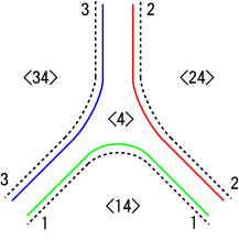
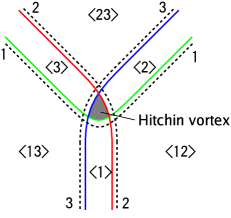
(a) Abelian junction		(b) non-Abelian junction

Figure 2: Internal structures of the junctions with $g\sqrt{c}\ll|\Delta m+i\Delta n|$

The Abelian junction shown in Fig. 2(a) separates the three different Higgs vacua $\langle 14\rangle$, $\langle 24\rangle$ and $\langle 34\rangle$. In the limit with $g\sqrt{c}\ll|\Delta m+i\Delta n|$, each component domain wall of the junction has internal structure (three-layer structure) as explained in Fig. 1(a). The same $U(1)$ subgroup is recovered in all three middle layers, as denoted by $\langle 4\rangle$. They are connected at the junction point so that the middle layer of the wall junction is also in the same phase $\langle 4\rangle$ as can be seen in Fig. 2(a). The Abelian junction charge $Y$ given in Eq.(4) gives always a negative contribution to the energy density [4], which can be understood as binding energy of the walls.

On the other hand, the non-Abelian junction has a complicated internal structure as shown in Fig. 2(b). Although it also separates three different vacua $\langle 12\rangle$, $\langle 23\rangle$ and $\langle 13\rangle$, their middle layers preserve different $U(1)$ subgroups, $\langle 1\rangle$, $\langle 2\rangle$ and $\langle 3\rangle$ as in Fig. 2(b). However, all the Higgs fields (hypermultiplets) vanish when all three middle layers overlap near the junction point so that only the $U(2)$ vector multiplet scalar $\Sigma$ is nonvanishing there. The $SU(2)$ part of this $\Sigma$ is responsible for the “positive” $Y$-charge which might be somewhat surprising because $Y$-charges were negative in all the junctions that have been constructed so far [6, 4]. Since such a positive contribution cannot be interpreted as binding energy, we wish to give another understanding. The key observation is that the 1/4 BPS equations given in Eq.(3) include the 1/2 BPS Hitchin equations

$$F_{12}=i\left[\Sigma_{1},\Sigma_{2}\right],\quad\mathcal{D}_{1}\Sigma_{2}-\mathcal{D}_{2}\Sigma_{1}=0,\quad\mathcal{D}_{1}\Sigma_{1}+\mathcal{D}_{2}\Sigma_{2}=0$$ (5)

of the Hitchin system, if we take the traceless part of Eq.(3) and ignore the hypermultiplet (Higgs) scalars. This reduction occurs at the core of the non-Abelian junction, since hypermultiplet scalars vanish and hence $U(1)$ and $SU(2)$ part of $U(2)$ decouple. Therefore the system reduces to the Hitchin system of $SU(2)$ subgroup in the middle of the non-Abelian junction. Furthermore, the $Y$-charge in Eq.(4) completely agrees with the charge the Hitchin system [7]. Now we can realize that the positive $Y$-charges of the non-Abelian junctions are the charges of the Hitchin system. One might suspect that such solution is not regular because the adjoint scalars of Eq.(5) grow exponentially and their charges diverge [12]. However, as we show below, the $Y$-charge for the non-Abelian junctions is finite because the adjoint scalar is out of the vacuum value only in a finite region around the junction point.

Let us next explicitly show that the Abelian junction has negative $Y$-charge whereas the non-Abelian junction has positive $Y$-charge. We found that domain walls and their junctions in the Abelian gauge theory are naturally described in the complex $\Sigma$ plane [4]. In that plane the SUSY vacuum $\langle A\rangle$ is expressed by a point $\mu_{A}$ and a wall interpolating between vacua $\langle A\rangle$ and $\langle B\rangle$ is by a segment between two points $\mu_{A}$ and $\mu_{B}$. A diagram made of these points and segments is called the grid diagram. Furthermore, the 3-pronged junction which divides three vacua $\langle A\rangle$, $\langle B\rangle$ and $\langle C\rangle$ corresponds to a triangle $\triangle ABC$ in that plane. In the previous paper [4] we showed that the $Y$-charge of the Abelian junction is negative and its magnitude is proportional to the area of the triangle. Here we again show this fact by a little bit different way. To this end, first we rewrite the $Y$-charge in Eq.(4) by using the Stokes theorem as

$$Y=-\frac{2}{g^{2}}\oint dx^{\alpha}\ {\rm Tr}\left(\Sigma_{1}\overset{\leftrightarrow}{\mathcal{D}}_{\alpha}\Sigma_{2}\right).$$ (6)

We consider the model with $N_{\rm F}=3$ and name three vacua $\langle 1\rangle$, $\langle 2\rangle$ and $\langle 3\rangle$ counterclockwisely as in Fig. 3(a).

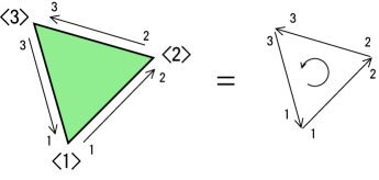
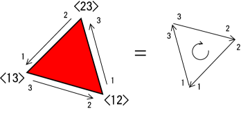
(a) Abelian junction		(b) non-Abelian junction

Figure 3: grid diagram and their orientation

The 1/4 BPS junction consists of three 1/2 BPS domain walls, so it can be dealt with as a collection of the 1/2 BPS walls in the contour integral (6) at three spatial infinities. Therefore the contour integral becomes the sum of the three line integrals

$$\oint dx^{\alpha}\ \Sigma_{1}\overset{\leftrightarrow}{\partial}_{\alpha}\Sigma_{2}=\sum_{A=1}^{3}T_{\left<A\right>\to\left<A+1\right>},\qquad T_{\left<A\right>\to\left<A+1\right>}\equiv\int_{\left<A\right>}^{\left<A+1\right>}\!\!dx^{\alpha}\ \Sigma_{1}\overset{\leftrightarrow}{\partial}_{\alpha}\Sigma_{2},$$ (7)

with identifying $\left<4\right>=\left<1\right>$. Here the integral $\int_{\left<A\right>}^{\left<A+1\right>}$ symbolically expresses the line integral on the line parallel to the vector $\vec{n}=(m_{A+1}-m_{A},n_{A+1}-n_{A})$. Although we cannot exactly solve the 1/2 BPS equation for the finite gauge coupling, it is enough to recall that 1/2 BPS solutions are mapped into segments between vacua $\mu_{A}$ and $\mu_{A+1}$ in the complex $\Sigma$ plane. Then the 1/2 BPS wall solution interpolating between vacua $\langle A\rangle$ and $\langle A+1\rangle$ can be written as

$$\Sigma_{\langle A\rangle\to\langle A+1\rangle}^{U(1)}=(\mu_{A+1}-\mu_{A})\rho(x^{\alpha})+\mu_{A},\quad W_{\alpha}=0.$$ (8)

with a real function $\rho(x^{\alpha})$ tending to $\rho(x^{\alpha})=0$ as $x^{\alpha}\to\langle A\rangle$ and $\rho(x^{\alpha})=1$ as $x^{\alpha}\to\langle A+1\rangle$. Plugging this into $T_{\left<A\right>\to\left<A+1\right>}$ in Eq.(7), we find $T_{\left<A\right>\to\left<A+1\right>}=\frac{1}{2}\vec{\mu}_{A}\times\vec{\mu}_{A+1}$, which is expressed as an exterior product of 2-vectors giving a scalar. Summing $T_{\left<A\right>\to\left<A+1\right>}$ over index $A$, we can verify that the $Y$-charge is negative and proportional to the area of the grid diagram

$$Y=-\frac{1}{g^{2}}\left(\vec{\mu}_{1}-\vec{\mu}_{3}\right)\times\left(\vec{\mu}_{2}-\vec{\mu}_{3}\right)=-\frac{2}{g^{2}}\times\left(\text{Area of grid diagram}\right).$$ (9)

Next let us focus on the non-Abelian junction. We consider $U(2)$ gauge theory with $N_{\rm F}=3$ flavors whose masses are the same with those in the Abelian gauge theory. There exist the three vacua $\langle 12\rangle$, $\langle 23\rangle$ and $\langle 31\rangle$ in this model. The grid diagrams in the complex $\Sigma$ plane for the Abelian gauge theory are naturally extended to diagrams in the ${\rm Tr}\Sigma$ plane for the non-Abelian gauge theories. In the ${\rm Tr}\Sigma$ plane the vacua $\langle\widetilde{A}\rangle=\langle BC\rangle$ $(\widetilde{A}\neq B\neq C)$ is a point at $\mu_{\widetilde{A}}=\mu_{B}+\mu_{C}$ and the 1/2 BPS walls correspond to segments between the two vertices. The non-Abelian junction corresponds to the triangle $\triangle{\widetilde{A}}{\widetilde{B}}{\widetilde{C}}$ in the plane. Notice that the triangle $\triangle{\widetilde{A}}{\widetilde{B}}{\widetilde{C}}$ for the non-Abelian junction and the triangle $\triangle ABC$ for the Abelian junction are congruent to each other and coincide when one of them is rotated by the angle $\pi$ [see Fig. 3(b)]. Furthermore, the orientation for the non-Abelian junction is opposite to the Abelian junction, namely it is clockwise. Similarly to the Abelian junction, we divide the contour integral in Eq.(6) into three line integrals as

$$\oint dx^{\alpha}\ {\rm Tr}\left(\Sigma_{1}\overset{\leftrightarrow}{\mathcal{D}}_{\alpha}\Sigma_{2}\right)=\sum_{\widetilde{A}=1}^{3}T_{\langle\widetilde{A}\rangle\to\langle\widetilde{A+1}\rangle},\quad T_{\langle\widetilde{A}\rangle\to\langle\widetilde{A+1}\rangle}\equiv\int^{\langle\widetilde{A+1}\rangle}_{\langle\widetilde{A}\rangle}\!\!dx^{\alpha}\ {\rm Tr}\left[\Sigma_{1}\overset{\leftrightarrow}{\mathcal{D}}_{\alpha}\Sigma_{2}\right],$$ (10)

with identifying $\langle\widetilde{4}\rangle=\langle\widetilde{1}\rangle$. In the each line integral the junction can be regarded as a 1/2 BPS single wall. The single wall interpolating between $\langle AB\rangle$ and $\langle BC\rangle$ can be obtained by embedding the solution of a single wall interpolating between $\langle A\rangle$ and $\langle C\rangle$ in the Abelian model [1] as

$$\Sigma_{\langle AB\rangle\to\langle BC\rangle}=\left(\begin{array}[]{cc}\Sigma^{U(1)}_{\langle A\rangle\to\langle C\rangle}&\\ &\mu_{B}\end{array}\right),\quad W_{\alpha}=0,$$ (13)

where $\Sigma^{U(1)}_{\langle A\rangle\to\langle C\rangle}$ is the solution of the single wall given in Eq.(8). Substituting this solution into Eq.(10), we find that $T_{\langle\widetilde{A}\rangle\to\langle\widetilde{A+1}\rangle}$ has a sign opposite to $T_{\langle A\rangle\to\langle{A+1}\rangle}$, because of the opposite orientation: $T_{\langle\widetilde{A}\rangle\to\langle\widetilde{A+1}\rangle}=T_{\langle A+1\rangle\to\langle A\rangle}=-T_{\langle A\rangle\to\langle{A+1}\rangle}$. Therefore we conclude that the $Y$-charge for the non-Abelian junction is positive and its magnitude agrees with the area of the grid diagram

$$Y=-\frac{2}{g^{2}}\sum_{\widetilde{A}=1}^{3}T_{\langle\widetilde{A}\rangle\to\langle\widetilde{A+1}\rangle}=\frac{2}{g^{2}}\times\left(\text{Area of grid diagram}\right).$$ (14)

For general $N_{\rm F}$ and $N_{\rm C}(<N_{\rm F})$ the webs of walls are constructed by the Abelian 3-pronged junction, the non-Abelian 3-pronged junction, and the intersection of penetrable walls (with vanishing $Y$-charge) as their building blocks. The rules for the grid diagrams in the $U(N_{\rm C})$ gauge theory are given as follows:

1. Determine mass arrangement $\mu_{A}$ and plot ${}_{N_{\rm F}}C_{N_{\rm C}}$ vacuum points $\langle A_{r}\rangle$ at $\sum_{r=1}^{N_{\rm C}}\mu_{A_{r}}$ in the complex ${\rm Tr}\Sigma$ plane.

2. Draw a convex polygon by choosing a set of vacuum points, which determines the boundary condition of a BPS solution. Here each edge of the convex polygon must be a 1/2 BPS single wall between pairs of the vacuum points $\langle\ \underline{\cdots}\ A\rangle$ and $\langle\ \underline{\cdots}\ B\rangle$.

3. Draw all possible internal segments within the convex polygon describing 1/2 BPS single walls forbidding any segments to cross.

4. Identify Abelian triangles with vertices $\langle\ \underline{\cdots}\ A\rangle$, $\langle\ \underline{\cdots}\ B\rangle$ and $\langle\ \underline{\cdots}\ C\rangle$ to Abelian 3-pronged junctions. Identify non-Abelian triangles with vertices $\langle\ \underline{\cdots}\ AB\rangle$, $\langle\ \underline{\cdots}\ BC\rangle$ and $\langle\ \underline{\cdots}\ CA\rangle$ to non-Abelian 3-pronged junctions. Identify parallelograms with vertices $\langle\ \underline{\cdots}\ AB\rangle$, $\langle\ \underline{\cdots}\ BC\rangle$, $\langle\ \underline{\cdots}\ CD\rangle$ and $\langle\ \underline{\cdots}\ DA\rangle$ to intersections of two penetrable walls with vanishing $Y$-charges.

Each grid diagram determines the topology of the web configuration and represents a subspace of the moduli space. The moduli of the web configurations are finally specified by drawing dual diagrams of the grid diagram, as illustrated by an example in Fig.4(a2) where the dashed line represents a dual diagram. Configurations with different topologies can be obtained by changing structure of internal segments and/or choosing other convex polygons. Thus the total moduli space of the web is obtained by gathering all possible grid diagrams.

The $U(2)$ gauge theory with four flavors gives the simplest example of wall webs containing both Abelian and non-Abelian junctions. According to mass arrangements for the hypermultiplets, the webs can be classified to two classes. Let us first consider a mass arrangement such as in the left figure of Fig. 4(a1).

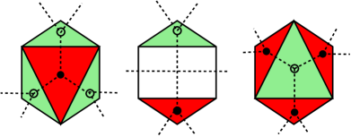
(a1) mass arrangement and vacua		(a2) grid diagrams and web configurations
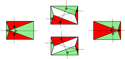
(b1) mass arrangement and vacua		(b2) grid diagrams and web configurations

Figure 4: (a1) and (a2) for the hexagon-type and (b1) and (b2) for the parallelogram-type web.

According to the rule i), vacuum points can be plotted in the ${\rm Tr}\Sigma$ plane as in the right figure of Fig. 4(a1). Moreover, we connect pairs of vertices corresponding to single walls under the rule iii), then we obtain the grid diagram for the web of walls. In Fig. 4(a2) we show three examples of the grid diagrams. Here light shaded (green) triangles are Abelian junctions and dark shaded (red) triangles are non-Abelian junctions while white parallelograms are intersections of penetrable walls (rule iv)). The dual diagrams in the configuration spaces are shown as the broken lines in Fig. 4(a2). These diagrams are transformed to each other by changing the moduli parameters of the solution as we show in the next section. The other class of the web configurations is obtained by the mass arrangement given in the left of Fig. 4(b1). According to the rule i), the vacuum points are plotted in the ${\rm Tr}\Sigma$ plane as in the right figure of Fig. 4(b1). By connecting the line between several pairs under the rule iii) and painting triangles two colors for Abelian and non-Abelian junctions, we get the grid diagrams. We show several examples in Fig. 4(b2). Unlike the above case, the grid diagram has 4 edges, so the web diagrams (shown by broken lines) has 4 external legs. These webs have a loop therein.

More complicated webs can easily be understood in terms of the grid diagrams in the complex ${\rm Tr}\Sigma$ plane. A web in the model of $(N_{\rm F},N_{\rm C})=(6,2)$ with ${}_{6}C_{2}=15$ vacua is shown in Fig. 5. The grid diagram has 6 edges, 9 Abelian triangles, 7 non-Abelian triangles and 3 parallelograms.

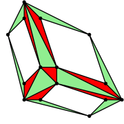
(a) mass arrangement and vacua		(b) grid diagram		(c) web diagram

Figure 5: The web of walls in the $U(2)$ gauge theory with 6 flavors.

Moduli and Configurations

Generic configurations of the 1/4 BPS webs are made of several Abelian and non-Abelian junctions. In order to investigate such generic webs more closely, we shall clarify the structure of the moduli parameters in generic solutions to Eq.(3). All the solutions of the 1/4 BPS equations can be expressed by matrices $S(x^{1},x^{2})$ and $H_{0}$, which is called the moduli matrix. The invertible $N_{\rm C}\times N_{\rm C}$ matrix $S$ is a function of $x^{1}$ and $x^{2}$, and $H_{0}$ is an $N_{\rm C}\times N_{\rm F}$ complex constant matrix with rank $N_{\rm C}$. Generic solutions to the first two equations in Eq. (3) are given in [4] by

$$H=S^{-1}H_{0}e^{M_{1}x^{1}+M_{2}x^{2}},\quad W_{\alpha}-i\Sigma_{\alpha}=-iS^{-1}\partial_{\alpha}S,\quad\left(\alpha=1,2\right).$$ (15)

The last equation of Eq.(3) can be rewritten into a gauge invariant equation, which is called the master equation [4] and determines $S$ for a given $H_{0}$ up to a gauge transformation. All the elements of the moduli matrix $H_{0}$ are integration constants, and can be moduli parameters in the solutions. However $(H_{0},S)\sim V(H_{0},S)$ with $V\in GL(N_{\rm C},{\bf C})$ gives the same physical fields in Eq.(15), and defines an equivalence relation which we call $V$-equivalence relation in what follows. Therefore we obtain the moduli space of the 1/4 BPS equations (3) to be the complex Grassmann manifold ${\cal M}_{\rm tot}\simeq G_{N_{\rm F},N_{\rm C}}=\{H_{0}\ |\ H_{0}\sim VH_{0},\ V\in GL(N_{\rm C},{\bf C})\}$. We call ${\cal M}_{\rm tot}$ the total moduli space because it contains all possible topological sectors of 1/2 and 1/4 BPS states and vacua (1/1 BPS) [4].

When a point in the moduli space $G_{N_{\rm F},N_{\rm C}}$ is given, we can figure out the configuration of the corresponding 1/4 BPS web as follows. The energy density of the web is approximately given in terms of the moduli matrix $H_{0}$ as

$${\cal E}\simeq\frac{c}{2}\left(\partial_{1}^{2}+\partial_{2}^{2}\right)\log\det\left(H_{0}e^{2(M_{1}x^{1}+M_{2}x^{2})}H_{0}^{\dagger}\right).$$ (16)

Notice that this expression is strictly correct for the strong coupling limit where we can exactly solve the 1/4 BPS equations (3) [4]. We can rewrite this expression in a more useful form

$${\cal E}=\frac{c}{2}\left(\partial_{1}^{2}+\partial_{2}^{2}\right)\log\sum_{\langle A_{r}\rangle}e^{2{\cal W}^{\langle A_{r}\rangle}},$$ (17)

where we define a linear function ${\cal W}^{\langle A_{r}\rangle}$ for each vacuum $\langle A_{r}\rangle$ as

$${\cal W}^{\langle A_{r}\rangle}(x^{1},x^{2})\equiv\sum_{r=1}^{N_{\rm C}}\left(m_{A_{r}}x^{1}+n_{A_{r}}x^{2}\right)+a^{\langle A_{r}\rangle}.$$ (18)

Here $e^{a^{\langle A_{r}\rangle}}$ gives the real part of the Plücker coordinates of $G_{N_{\rm F},N_{\rm C}}$, given by $\det H_{0}^{\langle A_{r}\rangle}$, where $H_{0}^{\langle A_{r}\rangle}$ is $N_{\rm C}\times N_{\rm C}$ matrix whose elements are given by $(H_{0}^{\langle A_{r}\rangle})^{s}{{}_{t}}=(H_{0})^{s}{{}_{A_{t}}}$:

$$a^{\langle A_{r}\rangle}+ib^{\langle A_{r}\rangle}\equiv\log\det H_{0}^{\langle A_{r}\rangle}.$$ (19)

We call $e^{{\cal W}^{\langle A_{r}\rangle}}$ in the logarithm in Eq.(17) the weight of the vacuum $\langle A_{r}\rangle$. For the vacuum configuration $\langle A_{r}\rangle$, all the weights of vacua except for the vacuum $\langle A_{r}\rangle$ vanishes. Therefore we find $\log\left(\sum e^{2{\cal W}}\right)=2{\cal W}^{\langle A_{r}\rangle}$ and then the energy density, of course, vanishes. When there are several domains of the vacua, domain walls appear as transition lines between the domains. At the vacuum domain $\langle A_{r}\rangle$ the weight $e^{{\cal W}^{\langle A_{r}\rangle}}$ is dominant compared to other weights. There $\log\left(\sum e^{2{\cal W}}\right)$ in Eq.(17) is an almost linear function $\log\left(\sum e^{2{\cal W}^{\langle A_{r}\rangle}}\right)\sim\max\left[\cdots,2{\cal W}^{\langle A_{r}\rangle},\cdots\right],$ so the energy density vanishes there. Only around transition lines between different domains, the energy density can have nonzero values. Thus positions of the single walls can be estimated by the condition of equating weights of the vacua. For example, the position of a single wall separating the two vacua $\langle\ \underline{\cdots}\ A\rangle$ and $\langle\ \underline{\cdots}\ B\rangle$ is given by the condition ${\cal W}^{\langle\underline{\cdots}A\rangle}={\cal W}^{\langle\underline{\cdots}B\rangle}$:

$$(m_{A}-m_{B})x^{1}+(n_{A}-n_{B})x^{2}+a^{\langle\underline{\cdots}A\rangle}-a^{\langle\underline{\cdots}B\rangle}=0.$$ (20)

The position of a 3-pronged junction can be estimated as an intersecting point of three lines (20) for the three constituent single walls of that junction. In other word, it can be estimated by equating three weights of vacua, like ${\cal W}^{\langle\underline{\cdots}A\rangle}={\cal W}^{\langle\underline{\cdots}B\rangle}={\cal W}^{\langle\underline{\cdots}C\rangle}$ for Abelian junctions or ${\cal W}^{\langle\underline{\cdots}AB\rangle}={\cal W}^{\langle\underline{\cdots}BC\rangle}={\cal W}^{\langle\underline{\cdots}AC\rangle}$ for non-Abelian junctions. Eq.(20) means that slopes of single walls are determined by mass differences between adjacent vacua, which agrees with the previous result of the central charge in Eq.(2). Besides slopes of walls, Eq.(20) contains additional data about positions of the single walls described by moduli $a^{\langle A_{r}\rangle}$. Thus we can attribute the deformation of the shape of the web to the change of the moduli parameters. To do this, however, one has to note that all the parameters $a^{\langle A_{r}\rangle}$ are not independent since the Plücker coordinates $\det H_{0}^{\langle A_{r}\rangle}$ must satisfy $2(_{N_{\rm F}}C_{N_{\rm C}}-1-N_{\rm C}(N_{\rm F}-N_{\rm C}))$ identities called the Plücker relations.

Examples: As a concrete example we examine the wall webs in the $N_{\rm F}=4,N_{\rm C}=2$ model in the rest of this paper. The $G_{4,2}$ can be embedded into ${\bf C}P^{5}$ with one Plücker relation and can be parameterized by six complex parameters $a^{\langle AB\rangle}+ib^{\langle AB\rangle}$ of homogeneous coordinates for ${\bf C}P^{5}$. Due to the $V$-equivalence relation and the Plücker relation, only four complex moduli parameters are independent. Notice that three out of eight real parameters are Nambu-Goldstone (NG) modes associated with the broken global $U(1)^{3}_{\rm F}$ symmetry. The remaining five parameters can change the shape of the web, but these three parameters do not.

First, let us examine the hexagon-type web of the walls with the mass parameters $M={\rm diag}(-\sqrt{3}-i,\sqrt{3}-i,2i,0)$ like webs given in Fig. 4(a), followed by the other type in Fig. 4(b). We start with the configuration given in Fig. 6(a) and denote the complex positions of the three outer Abelian junctions by $A_{1},A_{2},A_{3}$ and that of the center non-Abelian junction by $N_{0}$. The positions of the Abelian junctions are $A_{1}=\left(\frac{-a^{\langle 13\rangle}+3a^{\langle 14\rangle}-2a^{\langle 12\rangle}}{2\sqrt{3}},\frac{-a^{\langle 13\rangle}+a^{\langle 14\rangle}}{2}\right)$, $A_{2}=\left(\frac{a^{\langle 23\rangle}-3a^{\langle 24\rangle}+2a^{\langle 12\rangle}}{2\sqrt{3}},\frac{-a^{\langle 23\rangle}+a^{\langle 24\rangle}}{2}\right)$, $A_{3}=\left(\frac{-a^{\langle 23\rangle}+a^{\langle 13\rangle}}{2\sqrt{3}},\frac{a^{\langle 23\rangle}+a^{\langle 13\rangle}-2a^{\langle 34\rangle}}{2}\right)$ and that of the non-Abelian junctions is $N_{0}=\left(\frac{-a^{\langle 23\rangle}+a^{\langle 13\rangle}}{2\sqrt{3}},\frac{-a^{\langle 23\rangle}-a^{\langle 13\rangle}+2a^{\langle 12\rangle}}{6}\right)$. For simplicity, we fix the non-Abelian junction point $N_{0}$ at the origin, namely we fix $a^{\langle 12\rangle}=a^{\langle 23\rangle}=a^{\langle 13\rangle}$. By using the real part of the $GL(N_{\rm C},{\bf C})$ transformations for the $V$-equivalence relation, we can set these to zero. As a result we get $A_{1}=-a^{\langle 14\rangle}\left(-\frac{\sqrt{3}}{2},-\frac{1}{2}\right)$, $A_{2}=-a^{\langle 24\rangle}\left(\frac{\sqrt{3}}{2},-\frac{1}{2}\right)$, $A_{3}=-a^{\langle 34\rangle}\left(0,1\right)$ and $N_{0}=(0,0)$.

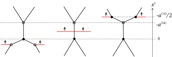
(a) A web configuration		(b) Changing moduli of the web

Figure 6: The web of walls for the hexagon-type mass arrangement.

Therefore $L_{*}\equiv-a^{\langle*4\rangle}$ gives the length of the arm $N_{0}A_{*}$, with “$*$” denoting $1,2,3$. These parameters have to satisfy the Plücker relation

$$e^{a^{\langle 34\rangle}+ib^{\langle 34\rangle}}-e^{a^{\langle 24\rangle}+ib^{\langle 24\rangle}}+e^{a^{\langle 14\rangle}+ib^{\langle 14\rangle}}=0,$$ (21)

where we fix NG mode coming from broken $U(1)_{\rm F}^{3}$ as $b^{\langle 12\rangle}=b^{\langle 23\rangle}=b^{\langle 13\rangle}=0$. Notice that the overall phase of the Plücker relation can be absorbed by the imaginary part of the $GL(N_{\rm C},{\bf C})$ transformations for the $V$-equivalence relation. At this stage the five parameters (position $N_{0}$ and $U(1)^{3}_{\rm F}$) have been fixed, and there still remain two constraints of the Plücker relation and possibility of the imaginary part of the $GL(N_{\rm C},{\bf C})$ transformations for the $V$-equivalence relation. As a result, we obtain three independent parameters out of six parameters $a^{\langle*4\rangle}$ and $b^{\langle*4\rangle}$. The physical meaning of the Plücker relation can be understood as follows. When the arms have comparable length $L_{1}\simeq L_{2}\simeq L_{3}>0$, the Plücker relation determines phases $b^{\langle 14\rangle},b^{\langle 24\rangle}$ and $b^{\langle 34\rangle}$ up to $V$-equivalence relation. In this case, as we expected before, the shape of the web can be freely changed by changing the parameters $a^{\langle*4\rangle}$. However, when one of the arms becomes extremely short, the situation drastically changes. For example, consider the situation where $L_{2}=0$ and $L_{1}\simeq L_{3}\gg 0$. Clearly such situation is forbidden by the Plücker relation since the left hand side of Eq.(21) is order one. The Plücker relation only allows that two out of three arms are simultaneously short, for example $L_{1}\simeq L_{2}\simeq 0$ while $L_{3}\gg 0$. This is a very big difference between the webs of $G_{4,2}$ and the webs of ${\bf C}P^{5}$ (with the same positions of vertices in its web diagram). In the case of the webs of ${\bf C}P^{5}$ the lengths of all arms are completely independent because no Plücker relations exist. Furthermore, one can connect two anti-podal vertices as shown by a dashed line in Fig. 7. Contrary to this ${\bf C}P^{5}$ case, this kind of configuration is forbidden in the case of the webs of $G_{4,2}$, because such segment is not a single domain wall anymore (compare Fig. 4(a) with Fig. 7). This is precisely a physical consequence of the Plücker relation.

Figure 7: A web configuration in ${\bf C}P^{5}$ model. This is forbidden for $G_{4,2}$ model.

Now we can easily show that there exist the deformation of the webs given in Fig. 4(a2). For simplicity, we set $a^{\langle 14\rangle}=a^{\langle 24\rangle}$ and fix $-a^{\langle 34\rangle}>0$ in the following. Depending on the value of $a^{\langle 14\rangle}$ there are three cases with completely different shapes of the webs as shown in Fig. 6(b): $a^{\langle 14\rangle}/2<0$, $0<a^{\langle 14\rangle}/2<-a^{\langle 34\rangle}$ and $-a^{\langle 34\rangle}<a^{\langle 14\rangle}/2$, respectively. There exist three outer Abelian and one non-Abelian junctions in the first case, one Abelian and one non-Abelian junctions and one intersection in the second case, and three outer non-Abelian and one Abelian junctions in the third case.

Next let us examine the parallelogram-type web with the mass parameters $M={\rm diag}(1/2-i,3/2,1/2+i,-3/2)$, like Fig. 4(b). The web graphs have four external legs as shown in Fig. 8. A characteristic feature of these diagrams have loops unlike the hexagon-type web. Here we concentrate on variation of shape of the web like Fig. 4(b2). The shapes of the loops are controlled by the weights $e^{{\cal W}^{\langle 13\rangle}}$ and $e^{{\cal W}^{\langle 24\rangle}}$ for the internal vacua $\langle 13\rangle$ and $\langle 24\rangle$. We start with the diagram in Fig. 8(a). To avoid inessential complications, we fix four external legs. This can be done by setting $a^{\langle 12\rangle}=a^{\langle 34\rangle}$, $a^{\langle 14\rangle}=a^{\langle 23\rangle}$ and fixing $L\equiv a^{\langle 12\rangle}+a^{\langle 34\rangle}-a^{\langle 14\rangle}-a^{\langle 23\rangle}$.

(a) A configuration		(b) Deformation of the loop in the web

Figure 8: The web diagrams in the parallelogram-type mass arrangement. Positions of the Abelian junction $A_{*}$ and the non-Abelian junction $N_{*}$ are given by $A_{1}=(s-1,-1),A_{2}=(\frac{2}{3},\frac{4}{3}+s),A_{3}=(\frac{1-s}{2},1),A_{4}=(-\frac{2}{3},-\frac{2}{3}-s),N_{1}=(1+s,1),N_{2}=(-\frac{2}{3},s-\frac{4}{3}),N_{3}=(-\frac{1+s}{2},-1),N_{4}=(\frac{2}{3},\frac{2}{3}-s)$ in unit of $\frac{L}{4}$.

The parameter $L$ determines the size of the loop. By using real part of the $GL(N_{\rm C},{\bf C})$ transformations for the $V$-equivalence relation, we can set $a^{\langle 12\rangle}=L/4$. Then positions of the four external legs are given by $x^{1}=\pm L/6$ and $x^{2}=\pm L/4$ as seen in Fig. 8. We also fix parameters $b^{\langle 12\rangle},b^{\langle 34\rangle},b^{\langle 14\rangle}$ and $b^{\langle 23\rangle}$. Note that $U(1)_{\rm F}^{3}$ act as $\delta b^{\langle AB\rangle}=\theta_{A}+\theta_{B}$ with $\sum_{A=1}^{4}\theta_{A}=0$. Then the imaginary part of the the $GL(N_{\rm C},{\bf C})$ transformations for the $V$-equivalence relation and two out of $U(1)^{3}_{\rm F}$ are fixed. Only one $U(1)_{\rm F}$ transformation defined by $\varphi/4\equiv\theta_{1}=-\theta_{2}=\theta_{3}=-\theta_{4}$ remains under the above fixing. The remaining moduli parameters are $a^{\langle 13\rangle}+ib^{\langle 13\rangle}=(u+v)L/4$ and $a^{\langle 24\rangle}+ib^{\langle 24\rangle}=(u-v)L/4$ $(u,v\in{\bf C})$ which control the shape of the loop. Notice that $u$ is invariant under the $\varphi$ transformation while $v$ transforms as $(L/2)\delta_{\varphi}v=i\varphi$. The imaginary part of $v$ is then the NG mode for the broken $U(1)_{\rm F}$ symmetry. The Plücker relation determines the parameter $u$ as

$$e^{\frac{L}{2}+i(b^{\langle 12\rangle}+b^{\langle 34\rangle})}-e^{\frac{L}{2}u}+e^{-\frac{L}{2}+i(b^{\langle 14\rangle}+b^{\langle 23\rangle})}=0.$$ (22)

In the following we consider that the size of the loop is sufficiently large, namely $L\gg 1$. This implies that $u\simeq 1$ holds ($u\simeq-1$ holds for $L\ll-1$). At this stage the web given in Fig. 8(b) is controlled by one moduli parameter $s\equiv{\rm Re}(v)$. In the parameter region $s<-1/3$, only the vacuum $\langle 24\rangle$ arises in the loop as in the left figure. The web has two Abelian junctions $A_{1}$ and $A_{3}$ and two non-Abelian junctions $N_{2}$ and $N_{4}$. When $s=-1/3$ holds, the Abelian junction $A_{3}$ and the non-Abelian junction $N_{4}$ get together, and they pass through each other when $s$ becomes larger than $-1/3$. In the parameter region where $-1/3<s<1/3$, both the vacua $\langle 24\rangle$ and $\langle 13\rangle$ appear in the loop as in the second figure. Here the web has two Abelian junctions $A_{1}$ and $A_{2}$ and two non-Abelian junctions $N_{1}$ and $N_{2}$. When $s=1/3$ holds, the Abelian junction $A_{1}$ and the non-Abelian junction $N_{2}$ get together. When $s$ is larger than $1/3$, the vacuum $\langle 24\rangle$ disappears in the loop. In the parameter region $s>1/3$ the web has two Abelian junctions $A_{2}$ and $A_{4}$ and two non-Abelian junctions $N_{1}$ and $N_{3}$ as in the third figure.

Notice that the value of the complex moduli parameter $v$ does not change the boundary condition of the web. Then we can consider the effective theory on the world volume of the web by promoting $v$ to a field $v(t,x^{3})$ whose real part deforms the loop and imaginary part is the NG mode for the broken $U(1)_{\rm F}$. Such effective theory is a 1+1 dimensional ${\cal N}=(2,0)$ SUSY sigma model [4, 7].

References

- [1] Y. Isozumi, M. Nitta, K. Ohashi and N. Sakai, Phys. Rev. Lett. 93, 161601 (2004) [arXiv:hep-th/0404198]; Phys. Rev. D 70, 125014 (2004) [arXiv:hep-th/0405194]; Phys. Rev. D 71, 065018 (2005) [arXiv:hep-th/0405129].
- [2] M. Eto, Y. Isozumi, M. Nitta, K. Ohashi, K. Ohta and N. Sakai, Phys. Rev. D 71, 125006 (2005) [arXiv:hep-th/0412024].
- [3] G. W. Gibbons and P. K. Townsend, Phys. Rev. Lett. 83, 1727 (1999) [arXiv:hep-th/9905196]; S. M. Carroll, S. Hellerman and M. Trodden, Phys. Rev. D 61, 065001 (2000) [arXiv:hep-th/9905217].
- [4] M. Eto, Y. Isozumi, M. Nitta, K. Ohashi and N. Sakai, “Webs of Walls,” arXiv:hep-th/0506135.
- [5] K. Kakimoto and N. Sakai, Phys. Rev. D 68, 065005 (2003) [arXiv:hep-th/0306077].
- [6] H. Oda, K. Ito, M. Naganuma and N. Sakai, Phys. Lett. B 471, 140 (1999) [arXiv:hep-th/9910095]; K. Ito, M. Naganuma, H. Oda and N. Sakai, Nucl. Phys. B 586, 231 (2000) [arXiv:hep-th/0004188]; Nucl. Phys. Proc. Suppl. 101, 304 (2001) [arXiv:hep-th/0012182]; M. A. Shifman and T. ter Veldhuis, Phys. Rev. D 62, 065004 (2000) [arXiv:hep-th/9912162]; M. Naganuma, M. Nitta and N. Sakai, Phys. Rev. D 65, 045016 (2002) [arXiv:hep-th/0108179].
- [7] M. Eto, Y. Isozumi, M. Nitta and K. Ohashi, “1/2, 1/4 and 1/8 BPS equations in SUSY Yang-Mills-Higgs systems: Field theoretical brane configurations,” arXiv:hep-th/0506257.
- [8] M. Arai, M. Nitta and N. Sakai, Prog. Theor. Phys. 113, 657 (2005) [arXiv:hep-th/0307274].
- [9] M. Shifman and A. Yung, Phys. Rev. D 67, 125007 (2003) [arXiv:hep-th/0212293].
- [10] A. Gorsky and M. A. Shifman, Phys. Rev. D 61, 085001 (2000) [arXiv:hep-th/9909015].
- [11] B. Chibisov and M. A. Shifman, Phys. Rev. D 56, 7990 (1997) [Erratum-ibid. D 58, 109901 (1998)] [arXiv:hep-th/9706141].
- [12] S. A. Cherkis and A. Kapustin, Commun. Math. Phys. 218, 333 (2001) [arXiv:hep-th/0006050].