Regular and chaotic interactions of two BPS dyons at low energy

Abstract

We identify and analyze quasiperiodic and chaotic motion patterns in the time evolution of a classical, non-Abelian Bogomol’nyi-Prasad-Sommerfield (BPS) dyon pair at low energies. This system is amenable to the geodesic approximation which restricts the underlying SU($2$) Yang-Mills-Higgs dynamics to an eight-dimensional phase space. We numerically calculate a representative set of long-time solutions to the corresponding Hamilton equations and analyze quasiperiodic and chaotic phase space regions by means of Poincaré surfaces of section, high-resolution power spectra and Lyapunov exponents. Our results provide clear evidence for both quasiperiodic and chaotic behavior and characterize it quantitatively. Indications for intermittency are also discussed.

I Introduction

The classical dynamics of non-Abelian gauge theories is known to be chaotic in a large part of its phase space bir94 . By itself this is not unexpected since chaos is far more the rule than the exception in nonlinear dynamical systems. Perhaps more surprising, however, is the mounting evidence for this chaotic behavior, which is strictly speaking a classical phenomenon, to be of relevance for physical quantum gauge theories as well.

Part of the existing indications for the chaoticity of non-Abelian gauge theories stem from “homogeneous approximations” which neglect all spatial variations of the fields. Although these drastic reductions of the dynamics access only a tiny and not generally physical fraction of the full phase space, the few remaining degrees of freedom proved sufficient to establish chaotic regimes first in SU$\left(2\right)$ Yang-Mills theory bas79 and later in Yang-Mills-Higgs theory mat81 and Chern-Simons gauge theory gia88 . Extensive lattice calculations of the time evolution under the full hyperbolic Yang-Mills equations subsequently showed that spatially inhomogeneous gauge fields not only evolve chaotically, too, but reveal even more complex and qualitatively new phenomena which are of direct physical relevance, for example, in nonequilibrium processes .

Between the above two computational extremes, i.e. either ad hoc truncations to only constant fields or the full solution of the classical field equations on the lattice, there exist physically interesting subsystems of the gauge dynamics whose spatially varying fields—typically soliton configurations—and time evolution can be studied without invoking uncontrolled approximations or requiring the solution of partial differential equations. In the following, we will focus on a prototypical such system, consisting of two electrically charged magnetic Bogomol’nyi-Prasad-Sommerfield (BPS) monopoles pra75 ; bog76 ; sut97 , i.e. dyons, whose nontrivial spatial extension gives rise to crucial properties including the magnetic charge. Nevertheless, the low-energy time evolution of the dyon pair is accurately described by the geodesic approximation which involves just a few collective degrees of freedom, governed by ordinary differential equations. This geodesic dynamics is one of the best understood examples for classical (and quantum) interactions between extended solutions of physically interesting 3+1 dimensional field theories and can be formulated at a rare level of explicitness GM:86 ; AH:88 . Beyond being fascinating in its own right (exhibiting e.g. the celebrated scattering angle $\pi/2$ for head-on collisions), it therefore serves as a paradigm for the interactions among many other physically important solitons . The purpose of the present paper is to examine regular and chaotic motion patterns of this system in a representative set of phase space regions.

Besides appearing in the electroweak sector of standard model extensions, monopoles and their potentially chaotic interactions may have a crucial function in the context of quark confinement by the strong interactions. This becomes most explicit in the central role which BPS monopoles play in the confinement mechanism of $N=2$ supersymmetric Yang-Mills theory in 3+1 dimensions sei94 . By condensing in the vacuum, they realize the classic ’t Hooft-Mandelstam dual superconductivity scenario tho76 in which color magnetic charges get screened while color electric charges are confined by the dual Meißner effect. Similar scenarios, in which the condensation of monopole-like objects plays a key role, are expected to unfold in more physical gauge theories as well . In 3+1 dimensional Yang-Mills theories, for example, there is lattice evidence for the condensation of Abelian-projected monopoles to generate the bulk of the string tension che97 . (According to an interesting recent suggestion, the “active” monopoles might actually be BPS dyon constituents of caloron solutions with nontrivial holonomy dia05 .) Hence monopoles may be instrumental in resolving the most profound remaining mystery of QCD, i.e. the quark confinement mechanism mil .

From a seemingly different but actually related perspective, quark confinement is expected to be linked to the chaotic behavior of classical chromodynamics as well. In fact, it has long been conjectured that the vacuum of non-Abelian gauge theories, when undergoing a transition from weakly to strongly coupled fields, also undergoes an order-disorder transition and that the strongly coupled QCD vacuum is populated by highly irregular color field configurations bir94 . In the limit of a large number of colors, in particular, a vacuum made of random Yang-Mills fields has been shown to be a necessary and sufficient condition for quark confinement ole82 . From the outset, one of the motivations for investigating chaos in non-Abelian gauge theories was therefore to shed light on its potential role in the confinement mechanism bas79 . Moreover, the instability of constant color-magnetic vacuum fields sav77 made it natural to conjecture that both gauge invariance and stability of the physical vacuum may be restored by disordering the color-magnetic background fields. Under the gluonic structures envisioned to carry the bulk of this disorder are random domains as well as populations of randomly distributed center vortices or monopoles.

The last of these scenarios may be related to the subject of our investigation. Indeed, it is tempting to speculate that a disordered ensemble of monopoles (and antimonopoles) in a semiclassical vacuum may be generated by chaotic low-energy interactions among the monopoles. In the following we are going to investigate precisely this type of interaction in the simplest possible setting, i.e. between just two BPS monopoles. One may then hope that the quantitative understanding of its chaotic regime will lead to new insights into the disorder of interacting monopole ensembles as well. For sufficiently dilute systems, expansions in the monopole density and more sophisticated many-body techniques might even provide a starting point for the quantitative treatment of chaotic multimonopole ensembles. Alternatively, one could contemplate the technically challenging extension of the geodesic approximation to approximate BPS multimonopole-multiantimonopole solutions which incorporate multimonopole interactions .

Based on the above motivations, our main objective in the following will be to deepen the qualitative and quantitative understanding of quasiperiodicity and chaos in the geodesic motion of two BPS dyons. The pioneering numerical studies of this motion in Refs. TR:88a ; TR:89 ; TRA:93 already provided several indications for its nonintegrability. (Evidence for chaotic fluctuations around single monopoles in SU$\left(2\right)$ Yang-Mills-Higgs theory exists as well joy92 , although not too large, minimally spherically symmetric excitations remain regular for04 .) After a brief recollection of the classical two-dyon dynamics at low energies, we will first extend previous studies by examining Poincaré sections for a set of numerically generated long-time trajectories of the dyon pair. In the subsequent sections we break new ground by invoking high-resolution power spectra and maximal Lyapunov exponents to analyze the dyon orbits further. This analysis will go beyond the mere identification of standard motion patterns and provide the first quantitative characterizations of quasiperiodic and chaotic two-dyon trajectories.

II Classical low-energy dynamics of the two-dyon system

In order to set the stage for our investigation, we first recapitulate some pertinent aspects of the dynamics of a classical BPS dyon pair at low energies and discuss its known constants of the motion. Readers interested in more detail are referred to the lucid discussion by Gibbons and Manton GM:86 .

We consider Yang-Mills-Higgs (YMH) theory in 3+1 dimensions with gauge group SU($2$) and the Higgs field in the adjoint representation, i.e. the Georgi-Glashow model. The classical field equations admit topological soliton solutions which are magnetic monopoles with integer magnetic charge $k$ tho74 . In the following we will be interested in these monopole solutions in the BPS limit of vanishing Higgs potential pra75 ; bog76 ; sut97 , which solve the more restrictive Bogomol’nyi equation bog76

$$B_{i}^{a}=\frac{1}{2}\varepsilon_{ijk}F_{jk}^{a}=\pm\left(\delta^{ac}\partial_{i}+g\varepsilon^{abc}A_{i}^{b}\right)\Phi^{c}$$ (1)

(where $F_{\mu\nu}^{a}$ is the field strength tensor of the gauge field $A_{\mu}^{a}$ and $\Phi^{a}$ is the (adjoint) Higgs field). The solutions of Eq. (1) are the absolute minima of the YMH energy in their topological charge sector and form a submanifold $M_{k}$ in the space of gauge-inequivalent finite-energy fields. Static multimonopole solutions (with $\left|k\right|>1$) of Eq. (1) are possible because the repulsive magnetic forces between the individual monopoles are counterbalanced by the attractive forces which the massless Higgs field mediates mon77 .

Although the underlying YMH dynamics is not directly embedded in the standard model, it appears naturally in grand-unified theories. Monopole solutions similar to the BPS prototype might therefore be physical. Their mass would probably be large enough to explain why they have so far escaped discovery in earthbound laboratories.

The monopole solutions come in families whose members are characterized by continuous collective coordinates or “moduli” $x^{\alpha}$. (For the one-monopole solution, for example, these are the three position coordinates of the center and an overall phase angle.) Hence the moduli space spanned by the collective coordinates is just the (generally curved) manifold $M_{k}$. Its metric $g_{\alpha\beta}\!\left(x\right)$ is induced by the metric on the more comprehensive space of all finite-energy field configurations which the kinetic terms in the YMH Lagrangian define.

The time evolution of a nonstatic and therefore in general electrically charged BPS monopole system is governed by the hyperbolic partial differential YMH equations whose quantitative analysis and solution poses rather formidable problems. Reassuringly, however, the low-energy dynamics of BPS dyons reduces to a much more tractable problem as long as Manton’s geodesic approximation NM:82 can be invoked. The latter rests on the observation that energy conservation forces the low-energy motion of the $k$-dyon system (with sufficiently small initial velocities of the collective coordinates, tangent to $M_{k}$) to remain close to one of the static BPS solutions on $M_{k}$ at all times. This is simply because $M_{k}$ contains all absolute YMH energy minima with magnetic charge $k$, so that moving out of it would cost both kinetic and potential energy. Hence the low-energy motion of a $k$-dyon system approximately corresponds to low-energy motion of an associated point on the moduli space $M_{k}$. Since the energy of all static $k$-monopole solutions is degenerate, i.e. at the same (minimal) potential, furthermore, the low-energy motion is approximately determined by the kinetic energy alone. Hence it corresponds to geodesic motion on the moduli space $M_{k}$, which is governed by the purely kinetic Lagrangian

$$L_{geod}=\frac{m}{2}g_{\alpha\beta}\!\left(x\right)\dot{x}^{\alpha}\dot{x}^{\beta},$$ (2)

where $m$ is the reduced mass of the dyons. Physically, this just means that at small velocities (compared to the velocity of light) internal excitations (vibrations) and deexcitations (radiation) can be neglected, i.e. the dyons adapt adiabatically to their interactions by deforming reversibly and scattering elastically. (Corrections to the geodesic approximation were analyzed in an effective field theory framework in Ref. bak98 .)

In the following, we will focus on the two-dyon system. Because of the product structure of the moduli space, its center of mass momentum and an overall phase (whose time dependence is associated with the total electric charge) are individually conserved, and their metric is flat. Hence those degrees of freedom decouple from the internal motion and can be separated out. The remaining dynamics simplifies to the geodesic motion in the four-dimensional internal part $M_{2}^{\left(0\right)}$ of the moduli space and can be studied independently. A physically intuitive coordinate system on $M_{2}^{\left(0\right)}$ consists of the Euler angles $\vartheta$, $\varphi$ and $\psi$, which determine the orientation of the two-dyon system , and the distance variable $\varrho$ which measures the separation between the two dyon centers (at large $\varrho$).

Although the metric on $M_{2}^{\left(0\right)}$ is induced by the SU$\left(2\right)$ YMH dynamics, its direct derivation from the kinetic terms of the YMH Lagrangian seems out of reach. Instead, it has been constructed on the basis of ingenious symmetry arguments by Atiyah and Hitchin (AH) AH:85 , as summarized in Appendix A. Specialization of Eq. (2) to the AH metric then determines the geodesic dynamics of the dyon pair explicitly. The resulting Lagrangian

$$L_{AH}=\frac{1}{2}\left[f^{2}\!\left(\varrho\right)\dot{\varrho}^{2}+a^{2}\!\left(\varrho\right)\omega_{x}^{2}+b^{2}\!\left(\varrho\right)\omega_{y}^{2}+c^{2}\!\left(\varrho\right)\omega_{z}^{2}\right]$$ (3)

turns out to be nonlinear since the AH metric is curved. The functions $a$, $b$, $c$ and $f$ of the separation $\varrho$ are given in Appendix A and the $\omega_{i}\!\left(\vartheta,\varphi,\psi\right)$ are angular velocities of the monopole (or dyon) pair around the axes of the body-fixed frame,

$$\omega_{x} =-\dot{\vartheta}\sin{\psi}\,+\dot{\varphi}\sin{\vartheta}\cos{\psi}\,,$$ (4)

$$\omega_{y} =\dot{\vartheta}\cos{\psi}\,+\dot{\varphi}\sin{\vartheta}\sin{\psi}\,,$$ (5)

$$\omega_{z} =\dot{\psi}+\dot{\varphi}\cos{\vartheta}\,.$$ (6)

The form of the Lagrangian (3) is analogous to that of a nonrigid body with distance-dependent “moments of inertia” $a^{2},b^{2}$ and $c^{2}$ around the body-fixed axes. Following Gibbons and Manton, we define the radial coordinate $\varrho$ by choosing $f=-b/\varrho$ which leads to convenient expressions for $a,b$ and $c$ GM:86 . In Appendix B, the four Euler-Lagrange equations of the geodesic motion are derived by variation of Eq. (3).

For the question of integrability versus chaos, the number of integrals of the motion plays a decisive role. In fact, a motion is (Liouville) integrable only if the number of independent conserved quantities (whose mutual Poisson brackets vanish) at least matches the number of degrees of freedom. For the geodesic dynamics (3), three constants of the motion are known explicitly (cf. Appendix B.2), namely, the total angular momentum

$$\mathcal{M}^{2}=p_{\vartheta}^{2}-2p_{\varphi}p_{\psi}\cot{\vartheta}\csc{\vartheta}+\left(p_{\varphi}^{2}+p_{\psi}^{2}\right)\csc^{2}{\!\vartheta}$$ (7)

(where the $p_{\alpha}$ are generalized momenta canonically conjugate to the coordinates $\alpha$, as defined in Eq. (40) of Appendix B), the energy (54) which, for geodesic motion, equals the Lagrangian since the potential on $M_{2}^{\left(0\right)}$ vanishes,

$$E_{AH}=\frac{1}{2}\left(\frac{p_{\varrho}^{2}}{f^{2}}+a^{2}\omega_{x}^{2}+b^{2}\omega_{y}^{2}+c^{2}\omega_{z}^{2}\right)$$ (8)

and, finally, the generalized momentum $p_{\varphi}$ conjugate to the coordinate $\varphi$ which is cyclic, i.e. does not appear explicitly in Eq. (3).

At least one additional, independent constant of the motion is therefore required for the two-dyon motion to become integrable. Such a fourth conserved quantity indeed exists (to arbitrarily good approximation) in at least one region of phase space, namely, where the two dyons remain infinitely separated. Since they cannot exchange electric charge then , the time evolution of each of their phases or, equivalently, their individual electric charge is conserved. Hence the motion of two far separated dyons must be integrable, as intuitively expected, and cannot exhibit chaos. (At asymptotic distances the AH metric reduces to the Euclidean Taub-NUT metric whose geodesic motion is indeed known to be integrable GM:86 ; vam96 .)

This situation changes, however, if the two dyons begin to approach each other. Only their total charge, but not their charge ratio, remains conserved since the dyons are then able to exchange charge through the Higgs field. (Even when starting asymptotically with two uncharged monopoles, one will therefore generally end up with two dyons of opposite but nonvanishing charge.) If the integral of the motion associated with the relative phase ceases to exist, chaotic motion becomes possible . It is this region of the phase space in which we will be particularly interested below.

The above observations raise the question for which orbits the violation of individual charge conservation can typically be considered as a small perturbation away from the integrable Taub-NUT limit. In our context, this question is of relevance because for such orbits the transition from integrable to chaotic motion will be delayed and potentially obscured by the implications of KAM theory. Indeed, the KAM theorem kam states that almost all invariant tori of the unperturbed Taub-NUT motion will remain intact during sufficiently small deviations from the $\varrho\rightarrow\infty$ limit . Under weakly nonintegrable perturbations the motion should therefore stay quasiperiodic for almost all initial conditions. Chaotic motion will then be restricted to the small set of trajectories which lie on the descendants of invariant tori with commensurate frequencies.

Although we have argued above that it is unlikely for the geodesic AH motion to be integrable outside of the asymptotic region, the existence of additional but so far undiscovered constants of the motion cannot be excluded a priori since no general method for finding all conserved quantities of a nonlinear dynamical system is available. Hence it was an important step by Temple-Raston and Alexander to gather the first numerical evidence for the existence of chaotic regions in the two-dyon phase space TR:88a ; TR:89 ; TRA:93 . In the next section, we will elaborate on part of these results by extending the Poincaré section analysis of Ref. TR:89 and by looking for orbits which bear the insignia of chaos.

III Poincaré sections

We begin our search for chaotic regions in the phase space of the dyon pair by analyzing the Poincaré sections of several typical trajectories. A Poincaré section draws a selective portrait of a given phase space orbit (over a finite time interval) which achieves an enormous data reduction by mapping the whole trajectory into a discrete set of points. This set transparently exhibits characteristic global aspects of the orbit and allows, in particular, a direct visual distinction between orbits which arise from integrable (or weakly nonintegrable, in the KAM sense) and fully nonintegrable dynamics.

Poincaré section analyses are most powerful for conservative systems with two degrees of freedom where a transparent graphical interpretation becomes possible. At first glance one might therefore doubt their utility in the eight-dimensional phase space of the two-dyon problem. However, in Ref. TR:89 it was recognized that a particular canonical transformation turns a second constant of the dyon pair motion (besides the generalized momentum $p_{\varphi}$), namely, the total angular momentum squared $\mathcal{M}^{2}$, into a canonical momentum. As a consequence, the transformed Hamiltonian becomes independent of the associated canonical variables while $p_{\varphi}$ and $\mathcal{M}^{2}$ act as fixed “external” parameters. This Hamiltonian actually defines a reduced, four-dimensional (and still symplectic) phase space in which $p_{\varphi}$ and $\mathcal{M}^{2}$ are automatically conserved at every point. Energy conservation further constrains all orbits to a three-dimensional hypersurface inside this reduced phase space and thus makes a graphical Poincaré section analysis feasible.

The Poincaré section of any given orbit is the set of its intersection points, in a fixed direction, with a suitable two-dimensional plane in phase space. In our case, a useful choice TR:89 is the $\left(\varrho,p_{\varrho}\right)$ plane located at the position $\mathcal{M}_{1}=0$ which we will adopt throughout. Hence we define the elements of an orbit’s Poincaré section as those points in which it pierces through this plane while $\mathcal{M}_{1}$ changes from positive to negative sign.

One can easily convince oneself that integrable and chaotic motions generate qualitatively different Poincaré sections. Indeed, the existence of an additional, fourth constant of the motion $C_{4}$ (as provided e.g. by $p_{\psi}$ for far separated dyons, cf. Appendix B.2) would restrict all orbits to a generally two-dimensional submanifold in phase space, namely, the intersection of the two three-dimensional hypersurfaces on which either the energy or $C_{4}$ have fixed values. The dyon-pair motion then becomes (Liouville) integrable, the submanifold becomes an invariant torus and the orbit’s intersection points with the $\left(\varrho,p_{\varrho}\right)$ plane sweep out a (maximally) one-dimensional curve. If the system is nonintegrable, on the other hand, no fourth constant of the motion exists and the orbit is only bound to the three-dimensional constant-energy surface (for strong enough nonintegrability in the KAM sense). Its intersection points with the $\left(\varrho,p_{\varrho}\right)$ plane can therefore be more broadly distributed and eventually fill a two-dimensional area, which provides a clear signature for a chaotic dynamical regime .

In order to prepare for the Poincaré section analysis, we have generated twelve representative orbits by numerically integrating the equations of motion (49)–(52) under suitable initial conditions . The latter are provided by specifying initial values for the four coordinates and their time derivatives. In order to facilitate the comparison with the results of Ref. TR:89 , we adopt the following five initial conditions, and the form of a sixth, at the initial time $t_{0}$:

$$\vartheta=\frac{\pi}{2},\hskip 14.22636pt\varphi=\psi=0,\hskip 14.22636pt\dot{\varrho}=\dot{\vartheta}=0\hskip 14.22636pt\text{and}\hskip 14.22636pt\dot{\varphi}=\frac{h_{2}}{a^{2}}.$$ (9)

As a consequence of Eqs. (40), the corresponding initial values of the conjugate momenta are

$$p_{\varrho}=0,\hskip 14.22636ptp_{\vartheta}=\mathcal{M}_{2}=0,\hskip 14.22636ptp_{\varphi}=\mathcal{M}_{1}=h_{2}\hskip 14.22636pt\text{and}\hskip 14.22636ptp_{\psi}=\mathcal{M}_{3}=c^{2}\dot{\psi},$$ (10)

which implies

$$\mathcal{M}^{2}\equiv\mathcal{M}_{1}^{2}+\mathcal{M}_{2}^{2}+\mathcal{M}_{3}^{2}=p_{\varphi}^{2}+p_{\vartheta}^{2}+p_{\psi}^{2}=h_{2}^{2}+c^{4}\dot{\psi}^{2}.$$ (11)

Here $h_{2}$ is the parameter in the reduced Hamiltonian which fixes the value of the conserved momentum $p_{\varphi}$. Hence only the initial values for $\dot{\psi}$ and $\varrho$ remain to be determined. If $h_{2}$ is given, Eq. (11) implies that the initial condition for $\dot{\psi}$ can be specified by fixing the value of another conserved quantity, namely, the total angular momentum squared $\mathcal{M}^{2}$. Finally, instead of prescribing the initial condition for $\varrho$ directly, it is more convenient to use the reparametrization

$$\varrho=2K\!\left(\sin{\!\frac{\beta}{2}}\right)$$ (12)

($K$ is an elliptic integral, cf. Eq. (37)), which maps infinite dyon separation ($\varrho\rightarrow\infty$) into $\beta=\pi$, and to specify the initial value of $\beta$. Under the above conditions (9), each orbit is therefore uniquely characterized by the values of $\beta$ and two integrals of the motion, $h_{2}$ and $\mathcal{M}^{2}$. For the interpretation of the results below it will be helpful to keep in mind that (at fixed $h_{2}$) the initial relative electric charge $p_{\psi}\!\left(t_{0}\right)$ of the two dyons, and therefore their initial Coulomb interaction, grows with $\mathcal{M}^{2}$ (cf. Eq. (11)).

A fourth-order Runge-Kutta algorithm GG:89 was used for the numerical integration of the equations of motion. The Eqs. (35) are solved along the way to obtain the values of the AH functions $a$, $b$ and $c$ at each $\varrho$. The length of an integration step was typically $10^{-4}$ and the longest runs contained $2^{27}$ steps. The accuracy of the generated orbits was monitored after each time step by calculating the three conserved quantities (i.e. $E$, $\mathcal{M}^{2}$ and $p_{\varphi}$). The maximal deviations from their fixed values were of the order $10^{-12}$. The Poincaré section of a given orbit is then constructed from those of its points at which $\mathcal{M}_{1}$ vanishes and $\mathcal{\dot{M}}_{1}<0$ . Since the numerical integration routine generates the orbits only at discrete time steps, the exact intersection points were determined by polynomial (Lagrange) interpolation between the two adjacent points on the orbit with opposite signs of $\mathcal{M}_{1}$.

We will now discuss the Poincaré sections for twelve orbits which all share the same $h_{2}$ value, $h_{2}=37.596$. We arrange them into three plots, each containing the sections of four orbits with a common value of $\mathcal{M}^{2}$ and initial values $\beta=\left(3.11,3.12,3.13,3.14\right)$ of the radial coordinate. The corresponding initial values for $\left(\varrho,p_{\varrho}\right)$ are indicated by a small circle although $\mathcal{M}_{1}=h_{2}\neq 0$ implies that they do not lie in the $\mathcal{M}_{1}=0$ plane. Each of the twelve selected orbits describes charged monopole, i.e. dyon interactions since $\mathcal{M}^{2}>h_{2}^{2}=\allowbreak 1413.5$ and Eq. (11) imply that the initial value of their momenta $p_{\psi}=c^{2}\dot{\psi}$, associated with the relative electric charge, is nonzero. The above initial conditions were chosen to yield a rather representative set of Poincaré sections similar to those considered in Ref. TR:89 , in order to both qualitatively confirm the results obtained there and to extend them into neighboring phase space regions.

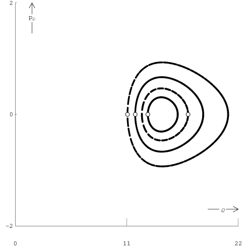
Figure 1: Poincaré sections, in the $(\varrho,p_{\varrho})$ plane located at the position $\mathcal{M}_{1}=0$, of four orbits from the Hamiltonian flow of Eq. (54) with $\mathcal{M}^{2}=1906.71$.

The first plot, Fig. 1, contains the four Poincaré sections with the smallest value $\mathcal{M}^{2}=1906.71$, i.e. with the weakest initial Coulomb attraction between the dyons. This explains why each of the orbits covers a rather large range of $\varrho$ values while the variation of the radial velocities, i.e. the $p_{\varrho}$ range, is relatively moderate. In three of the sections, furthermore, the two dyons never come closer than their initial distance, and in all four their separation $\varrho\gtrsim 11$ seems to stay well inside the asymptotic region where the relative charge of the dyons becomes (almost) time-independent and the motion (approximately or KAM-) integrable. This is confirmed by the Poincaré sections whose points indeed trace a one-dimensional closed curve which, within plot resolution, appears mostly continuous. Poincaré sections of this type are generated by superpositions of periodic motions with incommensurate frequencies, i.e. by quasiperiodic orbits. As discussed above, quasiperiodic behavior indicates that the dynamics is either integrable or at most weakly nonintegrable in the KAM sense.

In the next plot, Fig. 2, we display the analogous Poincaré sections with a larger value of $\mathcal{M}^{2}=2152.95$ and therefore with a stronger initial Coulomb attraction. Comparison with the sections of Fig. 1 shows that the variations in dyon distance are now smaller (tighter orbits) while their relative momenta vary more strongly over each of the orbits. The increased attraction also brings the dyons closer together, their maximal separation now being the initial one for all four orbits. Nevertheless, their minimal separation $\varrho_{\min}\sim 8$ seems to stay large enough for the motions to remain approximately integrable since all four Poincaré sections still form one-dimensional, closed curves.

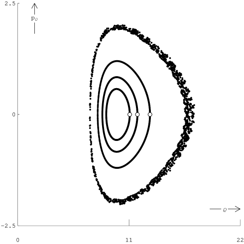
Figure 3: Same as Fig. 1 with $\mathcal{M}^{2}=2237.7$. (The outermost section contains about 13500 points.)

We therefore increase $\mathcal{M}^{2}$ further, to $\mathcal{M}^{2}=2237.70$, and plot the corresponding Poincaré sections in Fig. 3. Clearly, the character of the outermost section differs qualitatively from all those encountered previously. Instead of remaining constrained to a curve, it visibly spreads out into a two-dimensional area of the $\left(\varrho,p_{\varrho}\right)$ plane. Hence it corresponds to an aperiodic orbit and strongly suggests that the dynamics has become chaotic. This interpretation is consistent with the fact that the two dyons approach each other the most in this orbit. Their minimal distance $\varrho_{\min}\sim 2\pi$, which is about twice the distance of the bolt singularity at $\varrho=\pi$, apparently suffices for electric charge exchange by the Higgs field to become efficient and hence for $p_{\psi}$ to cease being even an approximate integral of the motion . This confirms earlier indications for the chaoticity of the geodesic two-dyon dynamics TR:88a which were supported by the analysis of similar Poincaré sections TR:89 , Julia sets TR:88b and escape plots of two-monopole scattering trajectories TRA:93 . An additional chaotic orbit, with a still larger value of $\mathcal{M}^{2}$, will be generated and analyzed in the following sections.

IV Power spectra

Numerical studies of a single chaos indicator are generally not sufficient to establish chaotic behavior with certainty. Inevitable numerical roundoff errors as well as specific features of a system under consideration (e.g. particular regions of instability) make it often desirable to probe the character of the motion by several complementary techniques. Typical pitfalls, like the premature misinterpretation of a seemingly irregular but perfectly integrable quasiperiodic motion pattern as chaos, can thereby be avoided.

Power spectral analysis has proven particularly useful for the distinction between (quasi-) periodic and chaotic time evolution GS:75;CFPS:80;LPC:81;BJ:87 . This is because the power spectra of ordered motion (either periodic or quasiperiodic) consist of sharp resonance lines which appear at simple harmonics of the base frequency in the periodic case and at any linear combination of all integer multiples of the base frequencies in the quasiperiodic case. Aperiodic systems, in contrast, are generally chaotic and have continuous and noisy power spectra.

In order to sharpen and extend the interpretation of the Poincaré section analysis of Sec. III, we have submitted the underlying orbit data to a spectral analysis. These data are four-dimensional, discrete time series of specific orbit solutions on $M_{2}^{\left(0\right)}$ whose coordinates $\left\{x^{\alpha}\!\left(t_{k}\right)\right\}=\left\{\vartheta,\varphi,\psi,\varrho\right\}$ are recorded numerically at equally spaced times $t_{k}:=k\Delta t$. Based on these solutions, one can calculate the time evolution of any dynamical variable $f\!\left(\left\{x^{\alpha}\!\left(t_{k}\right)\right\}\right)$ of interest as well as its discrete Fourier transform. We found it useful to choose the generalized momentum $p_{\varrho}\!\left(t_{k}\right)=f^{2}\!\left(\varrho\!\left(t_{k}\right)\right)\dot{\varrho}\!\left(t_{k}\right)$ conjugate to $\varrho$ as the dynamical variable. It has the power spectrum

$$P_{p_{\varrho}}\!\left(\nu\right)=\left|\frac{1}{\sqrt{N}}\sum_{k=0}^{N-1}p_{\varrho}\!\left(k\Delta t\right)e^{-2\pi ik\nu/N}\right|^{2}$$ (13)

which is a function of the mode frequencies $\nu$. (The Wiener-Khinchin theorem asserts that the alternative definition of $P\!\left(\nu\right)$ as the Fourier transform of the time series’ autocorrelation function is equivalent if the correlations decay sufficiently fast.) In order to assess a potential bias due to the choice of $p_{\varrho}$ as the dynamical variable, we have also calculated the power spectra associated with the time evolution of $\varrho$ and obtained essentially analogous results.

We numerically compute the power spectra by means of the Fast Fourier Transform algorithm. Appropriate windowing is used to suppress artificial oscillations due to the discrete data set and the finite time interval (see Ref. DK:00 and references therein). Since the impact of these artifacts decreases with the length of the time interval over which data for $p_{\varrho}\!\left(t_{k}\right)$ are available, we sample the orbits after each of $2^{25}$ time steps of length $\Delta t=10^{-4}$ which ensures sufficient accuracy for our purposes. We have calculated power spectra for the three orbits associated with the outermost Poincaré sections in each of the Figs. 1–3, specified by the initial conditions given in Sec. III, and for an additional orbit to be discussed below.

The $p_{\varrho}\!\left(t_{k}\right)$ time series based on the orbit associated with the outermost Poincaré section of Fig. 1 is depicted in Fig. 4a over $4\times 10^{6}$ time steps. The corresponding power spectrum (obtained from all data on $p_{\varrho}$, i.e. from the full orbit with $2^{25}$ time steps over a total time of $3.35\times 10^{3}$) is shown in a relatively small but representative frequency interval in Fig. 4e. On the basis of its Poincaré section, the underlying orbit was interpreted as quasiperiodic in Sec. III. The power spectrum confirms this interpretation but contains much more quantitative information. Indeed, while the underlying time series in Fig. 4a is in many ways indistinguishable from a periodic one, its power spectrum exhibits sharp peaks of varying strength which are located at odd integer linear combinations of two rationally independent (or incommensurate) base frequencies $\nu_{1}\simeq 0.0653$ and $\nu_{2}\simeq 0.0978$. Hence this orbit is two-mode quasiperiodic .

We now turn to the orbit whose Poincaré section is the outermost in Fig. 2. Again, its time series (cf. Fig. 4b) is visually difficult to distinguish from periodic motion while its power spectrum in Fig. 4f reveals a quasiperiodic motion with the two incommensurate base frequencies $\nu_{1}\simeq 0.1234$ and $\nu_{2}\simeq 0.1848$. In contrast to the previous power spectrum, however, the peaks at frequencies corresponding to more complex linear combinations of $\nu_{1}$ and $\nu_{2}$ are practically undetectable here. This seems to be a consequence of the larger initial coupling between the two dyons and is a rather frequent occurrence among sufficiently strongly interacting quasiperiodic systems. Although experimentally confirmed in many situations, a rigorous theoretical explanation for this type of behavior appears still to be missing ER:85 .

As foreshadowed by the results of the Poincaré section analysis, a strikingly different power spectrum is obtained from the orbit associated with the outermost section of Fig. 3. Indeed, this is the orbit whose Poincaré section indicated the chaoticity of the geodesic dynamics. Although the time dependence of its $p_{\varrho}$ in Fig. 4c remains, apart from small and irregular modulations, similar to the previous cases, the corresponding power spectrum in Fig. 4g has a qualitatively different character. Instead of sharp and isolated peaks, it now contains equally spaced, broadened peaks on top of a smooth and (within our frequency resolution) continuous background power distribution , covering all recorded frequencies and signalling the onset of aperiodicity .

The obvious departure from quasiperiodic behavior strengthens the evidence for the chaoticity of this orbit. Our discussion in Sec. II indicates, furthermore, that even the quasiperiodic behavior of the previous spectra, especially that of Fig. 4f, may have been generated by orbits which lie outside of the strictly integrable phase space region corresponding to asymptotically far separated dyons. Indeed, a discrete power spectrum still results if the nonintegrability is caused by weak perturbations and if the orbit remains on a KAM torus, i.e. continues to behave quasiperiodically . Our results imply that such a “delayed” onset of chaos might persist down to minimal distances $\varrho_{\min}\gtrsim 8$ between the two dyons.

In any case, the above findings suggest that the faster and closer the two dyons approach, the more unpredictable, i.e. chaotic their motion becomes. In order to test and extend this conclusion, we have calculated a further orbit with a still larger total angular momentum squared (and consequently stronger initial Coulomb interaction), $\mathcal{M}^{2}=2359.46$, and a somewhat smaller initial distance $\beta=3.13$ between the dyons than in the previous chaotic orbit. Its power spectrum, displayed in Fig. 4h, has a dense background and confirms the expectation that the new orbit is aperiodic as well. Comparison with the power spectrum of the first chaotic orbit shows, furthermore, that the background in Fig. 4h is less noisy and that more sharp frequencies remain clearly discernible than in Fig. 4g. The faster time dependence of the associated $p_{\varrho}\!\left(t\right)$ in Fig. 4d, on the other hand, exhibits more pronounced amplitude modulations. In the following section we will continue the analysis of the two chaotic orbits by calculating their maximal Lyapunov exponents.

One might perhaps wonder why we have encountered no quasiperiodic behavior with more than two fundamental modes. This is not particularly surprising, however, since two-mode quasiperiodicity is the rule rather than the exception among sufficiently strongly coupled, nonlinear dynamical systems. Indeed, the nonlinear couplings between an increasing number of modes tend to replace quasiperiodicity by chaos rue71 . It is quite plausible that this happens in the two-dyon system as well and explains the predominance of quasiperiodic orbits with the minimal number of two base frequencies.

In summary, our spectral analysis has uncovered that those parts of the two-dyon phase space which remain close enough to the asymptotic $\varrho\rightarrow\infty$ region are characterized by two-frequency quasiperiodic motion. In addition, we have determined the base frequencies of two typical quasiperiodic orbits quantitatively. Perhaps most importantly, the power spectra have also accomplished their main task to separate quasiperiodic from irregular behavior. In particular, they strongly support the identification of two orbits, the last one from Sec. III and an additional one with a still larger initial Coulomb force between the dyons, as chaotic. Our findings therefore substantially increase previous evidence that, apart from the asymptotic $\varrho\rightarrow\infty$ region, the relative low-energy motion of two BPS dyons admits only three independent conserved quantities and turns out to be genuinely nonintegrable.

While the distinction between (quasi-) periodic and chaotic motion is a particular strength of the spectral analysis, it does relatively little to further characterize chaotic behavior . Hence we consider it useful to subject our orbits to yet another classic analysis tool from the arsenal of chaos indicators, by calculating their characteristic or Lyapunov exponents. These exponents complement our previous analyses particularly well since they are specifically designed to quantify the chaoticity of irregular motion patterns.

V Lyapunov exponents

While the high-resolution spectral analysis of the last section has very clearly distinguished quasiperiodic from irregular orbits and determined the type of quasiperiodic behavior and its base frequencies quantitatively, it is much less specific about the properties of the aperiodic motion. It cannot, for example, unambiguously distinguish chaotic from (quasi-) random behavior (potentially due to roundoff errors).

Although previous work and our results of the last two sections have produced strong evidence for the chaoticity of two-dyon orbits in specific regions of the (finite $\varrho$) phase space, it therefore remains desirable to carry the investigation a step further and to obtain a quantitative characterization of the chaotic behavior. The most fundamental such characterization is provided by the values of positive Lyapunov exponents BGS:76 . After a brief and informal introduction to the underlying concepts, we will therefore evaluate the largest of these characteristic exponents for selected dyon pair orbits.

The primary function of Lyapunov exponents is to quantify the logarithmic rate of convergence or divergence between two orbits which started at an initial time $t_{0}$ at neighboring positions ${\mathbf{x}}_{0}$ and ${\mathbf{x}}_{0}+\delta{\mathbf{x}}_{0}$ (with $\lVert\delta{\mathbf{x}}_{0}\rVert\ll 1$ where $\lVert\cdot\rVert$ denotes the norm with respect to a Riemannian metric). Their relevance is obvious: exponentially divergent orbits, corresponding to positive Lyapunov exponents and signalling an exponential sensitivity of the time evolution to the initial conditions, are the prototypical signature of chaos. More specifically, under dynamical evolution for a sufficiently long time $t$ the deviation between the position of both orbits becomes $\delta{\mathbf{x}}_{t}$ and the maximal Lyapunov exponent $\mathsf{L}_{\text{max}}$ is defined by relating the deviation norms as $\lVert\delta{\mathbf{x}}_{t}\rVert\approx\exp\!\left(\mathsf{L}_{\text{max}}t\right)\lVert\delta{\mathbf{x}}_{0}\rVert$, i.e.

$$\mathsf{L}_{\text{max}}=\lim_{t\rightarrow\infty}\lim_{\lVert\delta{\mathbf{x}}_{0}\rVert\rightarrow 0}\frac{1}{t}\ln\!\frac{\lVert\delta{\mathbf{x}}_{t}\rVert}{\lVert\delta{\mathbf{x}}_{0}\rVert}.$$ (14)

For a detailed and rigorous treatment of Lyapunov exponents we refer to original work by Oseledec VIO:68 and Ruelle DR:79 , as well as to the review ER:85 .

Although the definition (14) of $\mathsf{L}_{\text{max}}$ is conceptually transparent, it does not lend itself to direct numerical implementation since in chaotic systems any initial deviation $\lVert\delta{\mathbf{x}}_{0}\rVert$, no matter how small, will eventually evolve into a number $\lVert\delta{\mathbf{x}}_{t}\rVert$ which far exceeds the (floating point) representation capabilities of computers. Hence more indirect numerical approaches are called for, and several different ones have been developed over the last decades JF:83;WSSV:85;SS:85;GK:87 . In the following, we will adopt the Jacobian method which integrates the equation for the time evolution of the deviation between two initially neighboring orbits, linearizing it anew at each time along the orbits and therefore having to manipulate only the relatively small deviations produced by one time step. A generalization of this method to the calculation of the whole non-negative Lyapunov spectrum was developed in Refs. BGGS:80 ; SN:79 . Our discussion and implementation follows Ref. MH:03 .

The Jacobian method is most transparently formulated by rewriting our system (49)–(52) of four second-order differential equations into a system of eight autonomous first-order equations

$$\dot{{\mathbf{x}}}\!\left(t\right)={\mathbf{F}}\!\left({\mathbf{x}}\!\left(t\right)\right),$$ (15)

where ${\mathbf{x}}$ comprises the four coordinates and their time derivatives, i.e. ${\mathbf{x}}$ and ${\mathbf{F}}$ are eight-dimensional column vectors. Under the initial conditions ${\mathbf{x}}\!\left(t_{0}=0\right)={\mathbf{x}}_{0}$, the unique solution of Eq. (15) is the orbit ${\mathbf{x}}\!\left(t\right)={\mathbf{\Phi}}\!\left(t,{\mathbf{x}}_{0}\right)$ with ${\mathbf{x}}_{0}={\mathbf{\Phi}}\!\left(0,{\mathbf{x}}_{0}\right)$. We now linearize the above system in the small deviation $\delta{\mathbf{x}}\!\left(t\right)$ at any point ${\mathbf{x}}\!\left(t\right)$ of the trajectory by substituting ${\mathbf{x}}\!\left(t\right)={\mathbf{x}}\!\left(t\right)+\delta{\mathbf{x}}\!\left(t\right)$ into Eq. (15) and neglecting terms of second-order in $\delta{\mathbf{x}}\!\left(t\right)$. The result is a linear system of first-order equations

$$\delta{\dot{\mathbf{x}}}\!\left(t\right)={\mathbf{J}}\!\left({\mathbf{x}}\!\left(t\right)\right)\!\cdot\mspace{1.0mu}\!\delta{\mathbf{x}}\!\left(t\right)$$ (16)

for the deviation $\delta{\mathbf{x}}$ which contains the Jacobi matrix ${\mathbf{J}}\!\left({\mathbf{x}}\!\left(t\right)\right)=\left[\partial{{\mathbf{F}}\!\left({\mathbf{x}}\right)}/\partial{{\mathbf{x}}}\right]\!|_{{\mathbf{x}}={\mathbf{x}\left(t\right)}}$. In terms of the tangent vector ${\boldsymbol{\xi}}\!\left(t\right)=\lim_{\lVert\delta{\mathbf{x}}\left(0\right)\rVert\rightarrow 0}\delta{\mathbf{x}}\!\left(t\right)\!/\lVert\delta{\mathbf{x}}\!\left(0\right)\mspace{1.82mu}\!\rVert$ on the orbit at ${\mathbf{x}}\!\left(t\right)$, Eq. (16) turns into the so-called variational system for ${\boldsymbol{\xi}}\!\left(t\right)$ under the initial data ${\mathbf{x}}_{0}$,

$${\dot{\boldsymbol{\xi}}}\!\left(t\right)={\mathbf{J}}\!\left({\mathbf{\Phi}}\!\left(t,{\mathbf{x}}_{0}\right)\right)\!\cdot\mspace{1.0mu}\!{\boldsymbol{\xi}}\!\left(t\right).$$ (17)

It propagates small variations tangent to the orbit at time $t_{0}$ to small variations tangent to the orbit at time $t$. In terms of the ${{\boldsymbol{\xi}}}$, Eq.${~{}\eqref{eqn:lcemax-def}}$ for ${\mathsf{L}_{\text{max}}}$ becomes

$$\mathsf{L}_{\text{max}}\!\left({\mathbf{x}}_{0},{\boldsymbol{\xi}}_{0}\right)=\lim_{t\rightarrow\infty}\chi\!\left(t\right)\text{ \ \ \ where \ \ \ \ }\chi\!\left(t\right):=\frac{\ln{\lVert{\boldsymbol{\xi}}\!\left(t\right)\mspace{1.82mu}\!\rVert}}{t}.$$ (18)

Hence, one can calculate $\mathsf{L}_{\text{max}}$ by numerically integrating the variational Eqs. (17) up to sufficiently large times. In order to supply the necessary input, i.e. the Jacobian ${\mathbf{J}}\!\left({\mathbf{\Phi}}\!\left(t,{\mathbf{x}}_{0}\right)\right)$ at each time step, one has to solve the equations of motion (15) for the orbit ${\mathbf{x}}\!\left(t\right)={\mathbf{\Phi}}\!\left(t,{\mathbf{x}}_{0}\right)$ in parallel. A biased choice for the initial tangent vector ${\boldsymbol{\xi}}_{0}$ is avoided by selecting its orientation randomly. The long-term time evolution of the orbits and ${{\boldsymbol{\xi}}\!}\left(t\right)$ will then be dominated by the largest Lyapunov exponent .

The numerical evaluation of Eq. (18) requires some additional precaution, however, since for chaotic orbits the norm ${\lVert{\boldsymbol{\xi}}\!}\left(t\right){\mspace{1.82mu}\!\!\rVert}$ will grow large enough to generate floating point overflows on computers. To circumvent these, we directly calculate the value of the required logarithmic norm after $n$ time steps ($t_{n}=n\Delta t$) as the sum

$$\ln{\lVert{\boldsymbol{\xi}}\!}\left(t_{n}\right){\mspace{1.82mu}\!\!\rVert}=\sum_{i=1}^{n}\ln\frac{{\lVert{\boldsymbol{\xi}}\!}\left(t_{i}\right){\mspace{1.82mu}\!\!\rVert}}{{\lVert{\boldsymbol{\xi}}\!}\left(t_{i-1}\right){\mspace{1.82mu}\!\!\rVert}}$$ (19)

(with ${\lVert{\boldsymbol{\xi}}\!}\left(t_{0}\right){\mspace{1.82mu}\!\!\rVert}=\lVert{\boldsymbol{\xi}}_{0}\mspace{1.82mu}\!\rVert=1$) of logarithmic length increments after each time step ras90 . The incremental norm changes ${\lVert{\boldsymbol{\xi}}\!}\left(t_{i}\right){\mspace{1.82mu}\!\!\rVert/\lVert{\boldsymbol{\xi}}\!}\left(t_{i-1}\right){\mspace{1.82mu}\!\!\rVert}$ remain small enough to be representable by floating point numbers and are obtained by renormalizing $\boldsymbol{\xi}$ to unit length after each evaluation. (Of course, the renormalized $\boldsymbol{\xi}$ remain solutions of the linear variational system (17).)

We now calculate, by means of the Jacobian technique, the maximal Lyapunov exponents of the four dyon-pair orbits whose power spectra were obtained in the last section and plotted in Figs. 4 e-h. The Poincaré sections of the first three of these orbits are the outermost in Figs. 1–3. The integration range consists of $n=2\times 10^{8}$ time steps which corresponds to approximately $650$ periods for the outermost quasiperiodic orbit of Fig. 1. In order to monitor the time evolution of $\chi$ during its approach to the limiting value $\mathsf{L}_{\text{max}}$ according to Eq. (18), we plot $\chi\!\left(t\right)$ for each of the four orbits in Fig. 5. Obviously, there is a striking qualitative difference between the plots for the two orbits which we had identified as (two-frequency) quasiperiodic in Sec. IV (with power spectra in Figs. 4e and 4f) and the irregular ones whose power spectra are shown in Figs. 4g and 4h. For the quasiperiodic orbits one infers within numerical uncertainties that $\mathsf{L}_{\text{max}}=\lim_{\,t\rightarrow\infty}\mspace{1.82mu}\!\chi\!\left(t\right)=0$ while $\chi\!\left(t\right)$ approaches the finite and positive values

$$\mathsf{L}_{\text{max,1}}\sim 0.02,\text{ \ \ \ \ \ \ }\mathsf{L}_{\text{max,2}}\sim 0.008$$ (20)

for the two aperiodic orbits. Around these orbits the motion is therefore exponentially sensitive to small variations of the initial conditions in at least one phase-space direction. This is the prototypical hallmark of chaos. We have thus achieved two of our main objectives, namely, the unequivocal confirmation of the chaoticity of the two-dyon system and a (semi-) quantitative determination of its primary characteristic scales.

The maximal Lyapunov exponent $\mathsf{L}_{\text{max,1}}$ of the first chaotic orbit (with the power spectrum in Fig. 4g) is more than twice as large as that of the second chaotic orbit (with the power spectrum in Fig. 4h), $\mathsf{L}_{\text{max,2}}$, although the differences in the initial conditions ($\mathcal{M}^{2}=2237.70$ and $\beta=3.14$ for the first and $\mathcal{M}^{2}=2359.46$ and $\beta=3.13$ for the second orbit) seem comparatively small. Closer inspection of these two orbits reveals that the minimal and maximal dyon distances in the first one are $\varrho_{\min,1}=6.99$ and $\varrho_{\max,1}=17.98$ while the corresponding momenta $p_{\varrho}$ vary inbetween $p_{\varrho,1\min/\max}=\pm 2.09$. For the second chaotic orbit one has a smaller variation between minimal and maximal $\varrho$ values, $\varrho_{\min,2}=6.73$ and $\varrho_{\max,2}=14.23$, and a somewhat smaller range of momenta, bounded by $p_{\varrho,2\min/\max}=\pm 1.94$. Although the initial Coulomb attraction between the dyons is stronger in the second orbit (since its total angular momentum squared $\mathcal{M}^{2}$ is 5% larger) and the dyons therefore come closer to each other and depart farther from the integrable asymptotic domain, its chaoticity—as measured by the maximal Lyapunov exponent—is still considerably smaller. This might be a consequence of the generally smaller momenta of the second orbit.

The behavior of $\chi$ also reveals a conspicuous qualitative difference between the two chaotic orbits. While the $\chi\!\left(t\right)$ of the first one (dot-dashed curve with filled triangles in Fig. 5) clearly stays above those of the quasiperiodic orbits for all $t$, the $\chi\!\left(t\right)$ of the second one (dashed curve with filled squares in Fig. 5) follows its quasiperiodic counterparts for a long time rather closely and then suddenly rises in a “burstlike” onset of chaos. This intriguing behavior may be a first vestige of intermittency in the geodesic dyon-pair motion. It also seems to explain the more regular and approximately quasiperiodic power spectrum of the second orbit [Fig. 4h]. Stronger evidence for the potentially intermittent behavior could be established by identifying complete intermittency intervals of $\chi\!\left(t\right)$ but would require much longer orbits. The power spectra of Sec. IV provide further testing grounds for intermittency which could be exploited, e.g., by subjecting them to a moment analysis or by searching for a power-law behavior in their low-frequency tails (i.e. $1/f$ noise) ben85 .

Although the large-time limit of $\chi\!\left(t\right)$ (i.e. the maximal Lyapunov exponent) vanishes for quasiperiodic orbits, its characteristic time dependence may contain useful information as well. In order to examine the behavior of $\chi\!\left(t\right)$ for quasiperiodic motion more closely, we select a new sample of three quasiperiodic orbits, namely, those whose Poincaré sections are the innermost in each of the Figs. 1–3, and display the corresponding $\chi\!\left(t\right)$ in Fig. 6. (The full (dotted, dash-dotted) line corresponds to the orbit with the innermost Poincaré section in Fig. 1 (2, 3).) At sufficiently large $t$ all curves seem to approach straight lines, which indicates a power-law behavior

$$\chi\!\left(t\right)\sim at^{-b}\text{ \ \ \ \ \ \ (}a,b>0\text{).}$$ (21)

This type of scaling behavior is frequently encountered in quasiperiodic systems and supports the visual impression that all curves have indeed the expected $\mathsf{L}_{\text{max}}=\lim_{\,t\rightarrow\infty}\mspace{1.82mu}\!\chi\!\left(t\right)=0$.

We close this section by recalling that (positive) maximal Lyapunov exponents contain crucial information about the physical behavior even of quantum systems. A notable example is their partial characterization of nonequilibrium processes in semiclassical systems (e.g. at high temperature) where they typically set the scale of relaxation times and thermalization rates hei97 . One might expect that our Lyapunov exponents play a similar role in determining, e.g., the equilibration rate of a nonequilibrium dyon system.

VI Summary and conclusions

We have analyzed several representative motion patterns of two interacting BPS dyons in the geodesic approximation. The main emphasis was put on discerning regular and chaotic orbits and on characterizing them both qualitatively and quantitatively by means of suitable chaos indicators.

Our study is based on a sample of thirteen long-time phase space trajectories for which four-dimensional time series were generated by numerically integrating the equations of motion with high accuracy over typically $2^{25}$ time steps. The initial data sets were chosen to cover a representative range of motion patterns and to explore the low-energy dyon interactions at different strengths. Hence the orbit set includes sequences of trajectories whose decreasing minimal dyon separations interpolate between asymptotic dyon distances, where charge exchange becomes ineffective and the geodesic dynamics integrable, and relatively small minimal separations for which the interactions are expected to become nonintegrable.

A second motive for our initial-data selection was to include orbits in the vicinity of those for which Poincaré sections were already available. This allows for a direct comparison with previous results and served as a useful benchmark and starting point for our work. We constructed Poincaré sections in the radial coordinate-momentum plane for twelve orbits. They qualitatively confirm the earlier results and extend them to trajectories in neighboring phase space regions. Moreover, they contain useful graphical information on the shape of the constant-energy surfaces and on the qualitative behavior of the two-dyon system as a function of the initial conditions. The dimensionality of the Poincaré sections, in particular, provides clear indications for the underlying trajectories to be either quasiperiodic or chaotic.

In order to complement the results of the Poincaré section analysis, we have additionally calculated high-resolution power spectra of selected orbits. The spectral analysis of the momentum conjugate to the dyon separation has provided particularly clean distinctions between quasiperiodic and aperiodic orbits which strengthen and extend the interpretation of the Poincaré sections. In addition, the power spectra produced the first quantitative characterization of quasiperiodic dyon-pair orbits by establishing the number of their fundamental modes (two), determining their frequencies and yielding the strength distribution over the various harmonics. The emergence of just the minimal, i.e. two-mode quasiperiodicity is rather widespread among sufficiently strongly coupled, nonlinear dynamical systems. The common expectation that nonlinear couplings between more than two fundamental modes increasingly turn quasiperiodicity into chaos might therefore apply to the two-dyon system as well and explain why we have only found two-mode-quasiperiodic and chaotic trajectories.

In contrast to their almost complete characterization of quasiperiodic motion patterns, power spectra do extract relatively little pertinent and quantitative information from irregular orbits. Hence we have additionally calculated the primary characteristic scales of chaotic motion, i.e. the maximal Lyapunov exponents, for a suitable subset of orbits. As expected, the Lyapunov exponents of orbits previously identified as quasiperiodic were found to vanish. The two orbits with an irregular broadband power spectrum, on the other hand, have finite and positive maximal Lyapunov exponents whose values were approximately determined as $\mathsf{L}_{\text{max,1}}\sim 0.02$ and $\mathsf{L}_{\text{max,2}}\sim 0.008$. Those provide our most unequivocal and quantitative evidence for the chaoticity of the dyon-dyon interactions. The orbit with the smaller Lyapunov exponent shows in addition signs of intermittent behavior.

Reassuringly, the results of all three employed analysis methods, i.e. Poincaré sections, power spectra and maximal Lyapunov exponents, are fully consistent with each other. Taken together, they provide convincing evidence for and a quantitative description of both quasiperiodic and chaotic regions in the low-energy phase space of two BPS dyons. Moreover, the integrability of noninteracting dyon systems allows to trace the origin of the chaotic behavior to the interactions between the dyons. These interactions may therefore help to disorder monopole ensembles similar to those which are expected to populate the vacuum of the strong interactions. In any case, our results imply that no more than the three explicitly known integrals of the motion are conserved by the geodesic forces between the dyons.

Appendix A Atiyah-Hitchin metric

In this appendix we establish our notation and briefly summarize pertinent features of the Atiyah-Hitchin (AH) metric and its Christoffel connection on the internal moduli space $M_{2}^{\left(0\right)}$ of the Bogomol’nyi-Prasad-Sommerfield (BPS) monopole pair. Full details can be found in the book AH:88 .

BPS magnetic monopoles are regular classical soliton solutions of the SU$\left(2\right)$ Yang-Mills-Higgs equations in the limit of vanishing Higgs self-coupling pra75 ; bog76 . The static two-monopole solutions define, as explained in Sec. II, the coollective-coordinate or moduli manifold $M_{2}^{\left(0\right)}$. Its metric was first written down explicitly by Atiyah and Hitchin AH:85 and determines the geodesic dynamics of two interacting BPS dyons at small velocities. The AH construction exploits the facts that the two-monopole moduli space is a hyper-Kähler (or Hamiltonian) manifold AH:88 ; JG:94 , that it admits SO($3$) as a group of isometries and that the orbits under the action of SO($3$) are with one exception three-dimensional. One can then show that the metric on $M_{2}^{\left(0\right)}$ must be of the form

$$ds^{2}=f^{2}d\varrho^{2}+\left(a^{2}l_{\alpha}l_{\beta}+b^{2}m_{\alpha}m_{\beta}+c^{2}n_{\alpha}n_{\beta}\right)dx^{\alpha}dx^{\beta},$$ (22)

where $a$, $b$, $c$ and $f$ are functions of the “radial” variable $\varrho$ only and $l_{\alpha}dx^{\alpha}$, $m_{\alpha}dx^{\alpha}$ and $n_{\alpha}dx^{\alpha}$ are differential forms on the three-sphere $S^{3}$ which can be taken as

$$\sigma_{1}:=l_{\alpha}dx^{\alpha}=-\sin{\psi}\,d\vartheta+\sin{\vartheta}\cos{\psi}\,d\varphi,$$

$$\sigma_{2}:=m_{\alpha}dx^{\alpha}=\cos{\psi}\,d\vartheta+\sin{\vartheta}\sin{\psi}\,d\varphi,$$

$$\sigma_{3}:=n_{\alpha}dx^{\alpha}=d\psi+\cos{\vartheta}\,d\varphi,$$ (23)

in terms of three Euler angles $\vartheta$, $\varphi$ and $\psi$ in the intervals $0\leq\vartheta\leq\pi$, $0\leq\varphi\leq 2\pi$, $0\leq\psi\leq 2\pi$. Accordingly, the two-monopole moduli space is parameterized by a coordinate $\varrho$ which describes the separation between the monopoles, two angular coordinates $\vartheta$ and $\varphi$ which determine the orientation of the axis that joins the monopoles, and the angle $\psi$ which fixes the position of the (generally axially asymmetric) two-monopole system with respect to rotations around this axis.

By casting the line element (22) into the Riemannian form $g_{\alpha\beta}\,dx^{\alpha}dx^{\beta}$, one can straightforwardly verify that the fundamental metric tensor $g_{\alpha\beta}$ is symmetric, i.e., $g_{\alpha\beta}=g_{\beta\alpha}$, and that the contravariant tensor $g^{\alpha\beta}$ is its inverse, $g_{\alpha\beta}\,g^{\beta\gamma}=\delta_{\alpha}{}^{\gamma}$, as it should be. Explicitly, the diagonal elements of $g_{\alpha\beta}$ read

$$g_{00} =f^{2},\text{ \ \ \ \ }g_{33}=c^{2},$$

$$g_{11} =a^{2}\sin^{2}{\!\psi}+b^{2}\cos^{2}{\!\psi},$$

$$g_{22} =a^{2}\sin^{2}{\!\vartheta}\cos^{2}{\!\psi}+b^{2}\sin^{2}{\!\vartheta}\sin^{2}{\!\psi}+c^{2}\cos^{2}{\!\vartheta},$$ (24)

while the nondiagonal ones are

$$g_{01} =g_{02}=g_{03}=g_{13}=0,$$

$$g_{12} =\left(b^{2}-a^{2}\right)\sin{\vartheta}\sin{\psi}\cos{\psi},$$

$$g_{23} =c^{2}\cos{\vartheta}.$$ (25)

Similarly, for the elements of the contravariant tensor $g^{\alpha\beta}$ one has

$$g^{00} =\frac{1}{f^{2}},\text{ \ \ \ \ }g^{33}=\frac{1}{c^{2}}+\left(\frac{\cos^{2}{\!\psi}}{a^{2}}+\frac{\sin^{2}{\!\psi}}{b^{2}}\right)\cot^{2}{\!\vartheta},$$

$$g^{11} =\frac{\cos^{2}{\!\psi}}{b^{2}}+\frac{\sin^{2}{\!\psi}}{a^{2}},$$

$$g^{22} =\left(\frac{\cos^{2}{\!\psi}}{a^{2}}+\frac{\sin^{2}{\!\psi}}{b^{2}}\right)\csc^{2}{\!\vartheta},$$ (26)

and

$$g^{01} =g^{02}=g^{03}=0,$$

$$g^{12} =\frac{\left(a^{2}-b^{2}\right)\csc{\vartheta}\sin{\psi}\cos{\psi}}{a^{2}b^{2}},$$

$$g^{13} =\frac{\left(b^{2}-a^{2}\right)\cot{\vartheta}\sin{\psi}\cos{\psi}}{a^{2}b^{2}},$$

$$g^{23} =-\left(\frac{\cos^{2}{\!\psi}}{a^{2}}+\frac{\sin^{2}{\!\psi}}{b^{2}}\right)\csc{\vartheta}\cot{\vartheta}.$$ (27)

With these expressions at hand, one can obtain explicit relations for the functions $a,$ $b,$ $c$ and $f$ by means of the equation

$$R_{\lambda\sigma}=\frac{\partial\Gamma^{\alpha}{}_{\lambda\sigma}}{\partial x^{\alpha}}-\frac{\partial\Gamma^{\alpha}{}_{\lambda\alpha}}{\partial x^{\sigma}}+\Gamma^{\alpha}{}_{\nu\alpha}\Gamma^{\nu}{}_{\lambda\sigma}-\Gamma^{\alpha}{}_{\nu\sigma}\Gamma^{\nu}{}_{\lambda\alpha}=0$$ (28)

for the symmetric second-rank tensor $R_{\lambda\sigma}$ which represents the fact that $M_{2}^{\left(0\right)}$ is hyper-Kähler. The $\Gamma^{\alpha}{}_{\lambda\sigma}$ are the components of the Christoffel connection, i.e. the Christoffel symbols of the second kind, which are related to the metric tensor by

$$\Gamma^{\alpha}{}_{\lambda\sigma}=\frac{1}{2}\,g^{\alpha\mu}\left(\frac{\partial g_{\sigma\mu}}{\partial x^{\lambda}}+\frac{\partial g_{\lambda\mu}}{\partial x^{\sigma}}-\frac{\partial g_{\lambda\sigma}}{\partial x^{\mu}}\right).$$ (29)

(Obviously, they are symmetric under exchange of the lower indices.) After inserting the expressions (24)–(27) for the elements of the metric into Eq. (28), one obtains the components of $R_{\lambda\sigma}$ as functions of $a,$ $b,$ $c$ and $f$:

$$R_{00}=\left(\frac{a^{\prime}}{a}+\frac{b^{\prime}}{b}+\frac{c^{\prime}}{c}\right)\frac{f^{\prime}}{f}-\frac{a^{\prime\prime}}{a}-\frac{b^{\prime\prime}}{b}-\frac{c^{\prime\prime}}{c}$$ (30)

(the prime denotes differentiation with respect to the coordinate $\varrho$) and

$$R_{11} =\Pi_{1}\sin^{2}{\!\psi}+\Pi_{2}\cos^{2}{\!\psi},$$

$$R_{12} =\left(\Pi_{2}-\Pi_{1}\right)\sin{\vartheta}\sin{\psi}\cos{\psi},$$

$$R_{22} =\left(\Pi_{1}\cos^{2}{\!\psi}+\Pi_{2}\sin^{2}{\!\psi}\right)\sin^{2}{\!\vartheta}+\Pi_{3}\cos^{2}{\!\vartheta},$$

$$R_{23} =\Pi_{3}\cos{\vartheta},\hskip 14.22636ptR_{33}=\Pi_{3},$$ (31)

where

$$\Pi_{1} =\frac{a^{4}-\left(b^{2}-c^{2}\right)^{2}}{2b^{2}c^{2}}+\left[\left(\frac{f^{\prime}}{f}-\frac{b^{\prime}}{b}-\frac{c^{\prime}}{c}\right)a^{\prime}-a^{\prime\prime}\right]\frac{a}{f^{2}},$$

$$\Pi_{2} =\frac{b^{4}-\left(a^{2}-c^{2}\right)^{2}}{2a^{2}c^{2}}+\left[\left(\frac{f^{\prime}}{f}-\frac{a^{\prime}}{a}-\frac{c^{\prime}}{c}\right)b^{\prime}-b^{\prime\prime}\right]\frac{b}{f^{2}},$$

$$\Pi_{3} =\frac{c^{4}-\left(a^{2}-b^{2}\right)^{2}}{2a^{2}b^{2}}+\left[\left(\frac{f^{\prime}}{f}-\frac{a^{\prime}}{a}-\frac{b^{\prime}}{b}\right)c^{\prime}-c^{\prime\prime}\right]\frac{c}{f^{2}}.$$ (32)

All other components of $R$ (with the exception of those which differ from the above by exchanging the indices) vanish. The equations (28) therefore reduce to

$$\Pi_{1}=0,\hskip 14.22636pt\Pi_{2}=0,\hskip 14.22636pt\Pi_{3}=0,$$ (33)

together with

$$\frac{a^{\prime}}{a}\frac{b^{\prime}}{b}+\frac{b^{\prime}}{b}\frac{c^{\prime}}{c}+\frac{c^{\prime}}{c}\frac{a^{\prime}}{a}=\frac{1}{2}\left(\frac{1}{a^{2}}+\frac{1}{b^{2}}+\frac{1}{c^{2}}-\frac{a^{4}+b^{4}+c^{4}}{2a^{2}b^{2}c^{2}}\right)f^{2}.$$ (34)

The last equation, however, is just a first integral of Eqs. (33) and may be regarded as a constraint imposed on the initial values of $a$, $b$, $c$ and its derivatives. The second-order equations, which of course conserve this constraint, can be obtained from each other by cyclic permutation of $\left(a,b,c\right)$. All four equations (33) and (34) together constitute the vacuum Einstein equations of the AH metric.

A particular set of first integrals of the second-order equations (33) are the first-order equation

$$\frac{2bc}{f}\frac{da}{d\varrho}=\left(b-c\right)^{2}-a^{2}$$ (35)

and the two others which are obtained from it by cyclical permutation of $\left(a,b,c\right)$. These differential equations for the functions $a$, $b$, $c$ and $f$ were first derived in Ref. BGPP:78 . They have been linearized and solved in terms of Legendre’s complete elliptic integrals of the first and second kind in Ref. AH:85 for $f=abc$ and in Ref. GM:86 for $f=-b/\varrho$. Below we will adopt the second choice, $f=-b/\varrho$, since it leads to expressions which are more convenient for our purposes. The explicit solution to Eq. (35) and its permutations is then GM:86

$$a^{2} =4K(K-E)(E-\bar{q}^{2}K)/E,$$

$$b^{2} =4KE(K-E)/(E-\bar{q}^{2}K),$$

$$c^{2} =4KE(E-\bar{q}^{2}K)/(K-E),$$ (36)

where

$$K\!\left(q\right)=\int_{0}^{\pi/2}d\tau\,(1-q^{2}\sin^{2}{\!\tau})^{-1/2},\hskip 14.22636ptE\!\left(q\right)=\int_{0}^{\pi/2}d\tau\,(1-q^{2}\sin^{2}{\!\tau})^{1/2}$$ (37)

are the complete elliptic integrals of the first and second kind, $q$ is related to $\varrho$ by $\varrho=2K(q)$ for $\pi\leq\varrho<\infty$ and $\bar{q}=\sqrt{1-q^{2}}$ is the conjugate modulus. At the value $\varrho=\pi$ (which implies $q=0$) the metric has a coordinate singularity, the so-called “bolt”, since $a(\pi)=0$ implies that the line element (22) becomes independent of $\sigma_{1}$.

Appendix B Equations and integrals of motion

B.1 Lagrange equations of motion

The geodesic low-energy dynamics of the two-dyon system is governed by the Lagrangian

$$L=\frac{m}{2}g_{\alpha\beta}\dot{x}^{\alpha}\dot{x}^{\beta}=\frac{1}{2}\left(f^{2}\dot{\varrho}^{2}+a^{2}\omega_{x}^{2}+b^{2}\omega_{y}^{2}+c^{2}\omega_{z}^{2}\right),$$ (38)

where the reduced mass $m$ of the dyon-pair has been set to $m=1$ (instead of $m=2\pi$ in Ref. GM:86 ). The first equation in (38) describes generic geodesic motion while the second one is specialized to the Atiyah-Hitchin metric on the internal collective coordinate manifold $M_{2}^{\left(0\right)}$ in terms of the functions $a$, $b$, $c$ and $f$. The components $\omega_{x}$, $\omega_{y}$ and $\omega_{z}$ of the instantaneous (or “body-fixed”) angular velocity $\vec{\omega}$ along the axes $x$, $y$ and $z$ may be expressed in terms of the rates of change of the Euler angles as

$$\omega_{x}\equiv\sigma_{1}/dt,\hskip 14.22636pt\omega_{y}\equiv\sigma_{2}/dt,\hskip 14.22636pt\omega_{z}\equiv\sigma_{3}/dt$$ (39)

(cf. Eq. (23)). The canonically conjugate momenta associated with the four relative coordinates $\varrho$, $\vartheta$, $\varphi$ and $\psi$ are

$$p_{\varrho} =f^{2}\dot{\varrho},\hskip 14.22636ptp_{\psi}=c^{2}\omega_{z},$$

$$p_{\vartheta} =b^{2}\omega_{y}\cos{\psi}-a^{2}\omega_{x}\sin{\psi},$$

$$p_{\varphi} =a^{2}\omega_{x}\sin{\vartheta}\cos{\psi}+b^{2}\omega_{y}\sin{\vartheta}\sin{\psi}+c^{2}\omega_{z}\cos{\vartheta}.$$ (40)

The Euler-Lagrange equations for the time evolution of the collective coordinates are obtained by varying the action based on the Lagrangian (38). Variation with respect to the radial coordinate $\varrho\!\left(t\right)$ leads to

$$f^{2}\ddot{\varrho}+ff^{\prime}\dot{\varrho}^{2}-a\,a^{\prime}\omega_{x}^{2}-b\,b^{\prime}\omega_{y}^{2}-c\,c^{\prime}\omega_{z}^{2}=0,$$ (41)

while the equation of motion for the coordinate $\psi\!\left(t\right)$ becomes

$$2\mspace{1.5mu}c\,c^{\prime}\omega_{z}\dot{\varrho}+c^{2}\dot{\omega}_{z}=\left(a^{-2}-b^{-2}\right)a^{2}b^{2}\omega_{x}\omega_{y}.$$ (42)

The remaining two equations of motion for $\varphi\!\left(t\right)$ and $\vartheta\!\left(t\right)$ are

$$2\mspace{1.5mu}b\,b^{\prime}\omega_{y}\dot{\varrho}\cos\psi-2\mspace{1.5mu}a\,a^{\prime}\omega_{x}\dot{\varrho}\sin\psi+c^{2}\omega_{z}\dot{\varphi}\sin\vartheta$$ (43)

$$= \left(\dot{\omega}_{x}\sin{\psi}+\omega_{x}\omega_{z}\cos{\psi}\right)a^{2}-\left(\dot{\omega}_{y}\cos{\psi}-\omega_{y}\omega_{z}\sin{\psi}\right)b^{2}$$

and

$$2\mspace{1.5mu}a\,a^{\prime}\omega_{x}\dot{\varrho}\sin\vartheta\cos\psi+2\mspace{1.5mu}b\,b^{\prime}\omega_{y}\dot{\varrho}\sin\vartheta\sin\psi+2\mspace{1.5mu}c\,c^{\prime}\omega_{z}\dot{\varrho}\cos\vartheta$$ (44)

$$= \bigl{[}\bigl{(}\dot{\psi}\sin{\vartheta}\sin{\psi}-\dot{\vartheta}\cos{\vartheta}\cos{\psi}\bigr{)}\mspace{1.5mu}\omega_{x}-\dot{\omega}_{x}\sin{\vartheta}\cos{\psi}\bigr{]}a^{2}$$

$$-\mspace{4.75mu}\bigl{[}\bigl{(}\dot{\psi}\sin{\vartheta}\cos{\psi}+\dot{\vartheta}\cos{\vartheta}\sin{\psi}\bigr{)}\mspace{1.5mu}\omega_{y}+\dot{\omega}_{y}\sin{\vartheta}\sin{\psi}\bigr{]}b^{2}$$

$$+\mspace{5.85mu}\bigl{(}\omega_{z}\dot{\vartheta}\sin{\vartheta}-\dot{\omega}_{z}\cos{\vartheta}\bigr{)}\mspace{1.25mu}c^{2}.$$

A pair of equations which are algebraic consequences of Eqs. (43) and (44),

$$2\mspace{1.5mu}b\,b^{\prime}\omega_{y}\dot{\varrho}+b^{2}\dot{\omega}_{y} =\left(c^{-2}-a^{-2}\right)a^{2}c^{2}\omega_{x}\omega_{z},$$ (45)

$$2\mspace{1.5mu}a\,a^{\prime}\omega_{x}\dot{\varrho}+a^{2}\dot{\omega}_{x} =\left(b^{-2}-c^{-2}\right)b^{2}c^{2}\omega_{y}\omega_{z},$$ (46)

will be helpful in arriving at a more efficient formulation. Indeed, with $\dot{\varrho}=p_{\varrho}/f^{2}$ one also has

$$\ddot{\varrho}=\frac{\dot{p}_{\varrho}f-2\mspace{1.5mu}p_{\varrho}\dot{\varrho}\mspace{1.5mu}f^{\prime}}{f^{3}}=\frac{\dot{p}_{\varrho}}{f^{2}}-\frac{2\mspace{1.5mu}p_{\varrho}^{2}\mspace{1.5mu}f^{\prime}}{f^{5}}$$ (47)

and, introducing the ($\varrho$-dependently) rescaled angular velocities (in the body-fixed frame)

$$\mathcal{M}_{1}=a^{2}\omega_{x},\hskip 21.33955pt\mathcal{M}_{2}=b^{2}\omega_{y},\hskip 21.33955pt\mathcal{M}_{3}=c^{2}\omega_{z},$$ (48)

one can rewrite the four equations of (relative) motion concisely as

$$\dot{\mathcal{M}}_{1} =\left(\frac{1}{b^{2}}-\frac{1}{c^{2}}\right)\mathcal{M}_{2}\,\mathcal{M}_{3},$$ (49)

$$\dot{\mathcal{M}}_{2} =\left(\frac{1}{c^{2}}-\frac{1}{a^{2}}\right)\mathcal{M}_{3}\,\mathcal{M}_{1},$$ (50)

$$\dot{\mathcal{M}}_{3} =\left(\frac{1}{a^{2}}-\frac{1}{b^{2}}\right)\mathcal{M}_{1}\,\mathcal{M}_{2},$$ (51)

$$\dot{p}_{\varrho} =\frac{p_{\varrho}^{2}\mspace{1.5mu}f^{\prime}}{f^{3}}+\mathcal{M}_{1}^{2}\,\frac{a^{\prime}}{a^{3}}+\mathcal{M}_{2}^{2}\,\frac{b^{\prime}}{b^{3}}+\mathcal{M}_{3}^{2}\,\frac{c^{\prime}}{c^{3}}.$$ (52)

In this form, the equations of motion were first obtained in Refs. GM:86 ; BM:88 .

B.2 Integrals of the motion

Three independent constants of the geodesic Atiyah-Hitchin motion are known explicitly. The first one can be immediately identified by noting that $\varphi$ is a cyclic coordinate, i.e. that it does not appear explicitly in the Lagrangian (38). The corresponding generalized momentum $p_{\varphi}$ is therefore an integral of the motion, i.e. $\dot{p}_{\varphi}=0$.

The Hamiltonian $H$ is obtained by the standard Legendre transformation

$$H=p_{\varrho}\dot{\varrho}+p_{\vartheta}\dot{\vartheta}+p_{\varphi}\dot{\varphi}+p_{\psi}\dot{\psi}-L$$ (53)

of the Lagrangian (38). Using Eqs. (40) to express velocities in terms of coordinates and their conjugate generalized momenta, the Hamiltonian becomes

$$H = \frac{1}{2}\left[\frac{p_{\varrho}^{2}}{f^{2}}+\frac{p_{\psi}^{2}}{c^{2}}+\left(\frac{\cos^{2}{\!}\psi}{a^{2}}+\frac{\sin^{2}{\!}\psi}{b^{2}}\right)\left(p_{\varphi}\csc\vartheta-p_{\psi}\cot\vartheta\right)^{2}\right]$$ (54)

$$+\frac{p_{\vartheta}}{2}\left[\left(\frac{\sin^{2}{\!}\psi}{a^{2}}+\frac{\cos^{2}{\!}\psi}{b^{2}}\right)p_{\vartheta}+\frac{a^{2}-b^{2}}{a^{2}b^{2}}\left(p_{\varphi}\csc\vartheta-p_{\psi}\cot\vartheta\right)\sin\left(2\psi\right)\right],$$

which assumes the same values as the Lagrangian since both are of purely kinetic origin. Neither in $L$ nor, as a consequence, in $H$ does the time coordinate $t$ appear explicitly. The corresponding Hamilton equation, $\dot{H}=\left\{H,H\right\}=0$, therefore trivially implies that the total relative energy $H$ of the two-dyon system is conserved and furnishes a second integral of the motion.

The third constant of the motion is the square of the (both frame- and body-fixed) total angular momentum, $\mathcal{M}^{2}$, which can be expressed as the sum of the squares of the rescaled body-fixed angular velocities, i.e. $\mathcal{M}^{2}=\mathcal{M}_{1}^{2}+\mathcal{M}_{2}^{2}+\mathcal{M}_{3}^{2}$. One may check that $\mathcal{M}^{2}$ is conserved by adding up the equations obtained from multiplying Eq. (49) by $2\mathcal{M}_{1}$, Eq. (50) by $2\mathcal{M}_{2}$ and Eq. (51) by $2\mathcal{M}_{3}$. The result is

$$2\mathcal{M}_{1}\dot{\mathcal{M}}_{1}+2\mathcal{M}_{2}\dot{\mathcal{M}}_{2}+2\mathcal{M}_{3}\dot{\mathcal{M}}_{3}=0$$ (55)

and therefore

$$\frac{d}{dt}\mathcal{M}^{2}=0.$$ (56)

By using the explicit expressions

$$\mathcal{M}_{1}=\frac{p_{\varphi}\cos{\psi}-p_{\psi}\cos{\vartheta}\cos{\psi}-p_{\vartheta}\sin{\vartheta}\sin{\psi}}{\sin{\vartheta}},$$ (57)

$$\mathcal{M}_{2}=\frac{p_{\varphi}\sin{\psi}-p_{\psi}\cos{\vartheta}\sin{\psi}+p_{\vartheta}\sin{\vartheta}\cos{\psi}}{\sin{\vartheta}},$$ (58)

and

$$\mathcal{M}_{3}=p_{\psi}$$ (59)

for the rescaled angular velocities, one can re-express the total angular momentum squared in terms of the Euler angles and their canonically conjugate momenta as

$$\mathcal{M}^{2}=\sum_{j=1}^{3}\mathcal{M}_{j}^{2}=p_{\vartheta}^{2}-2p_{\varphi}p_{\psi}\cot{\vartheta}\csc{\vartheta}+\left(p_{\varphi}^{2}+p_{\psi}^{2}\right)\csc^{2}{\!\vartheta}.$$ (60)

For the investigation of chaos in the two-dyon system it is important to note that a fourth integral of the motion appears in the $\varrho\rightarrow\infty$ limit, i.e. if the dyons are far separated. Indeed, in this case the Atiyah-Hitchin metric simplifies to the Euclidean Taub-NUT metric GM:86 and the electric charge density, associated with the canonical momentum $p_{\psi}=c^{2}\omega_{z}$, becomes a fourth constant of the motion, i.e. $\dot{p}_{\psi}=0$.

The simple physical explanation of this result is that infinitely separated dyons cannot exchange electric charge, so that in addition to their overall charge also their individual charges become time-independent. In this case there exist at least four independently conserved quantities in the eight-dimensional phase space, enough to render the geodesic dynamics in Euclidean Taub-NUT space (Liouville-) integrable GM:86 . As a consequence, the asymptotic motion of two BPS dyons cannot be chaotic. Moreover, the potential transition from regular motion at $\varrho\rightarrow\infty$ to chaotic motion for finite, decreasing $\varrho$ may be “delayed” according to KAM theory kam by a stepwise dissolution of the invariant tori.

Figure 2: Same as Fig. 1 with $\mathcal{M}^{2}=2152.95$.

Figure 4: Panel a (b, c) shows the time dependence of $p_{\varrho}$ and panel e (f, g) the logarithm of the corresponding power spectrum for the dyon-pair orbit whose Poincaré section is plotted in Fig. 1 (2, 3). The panels d and h show $p_{\varrho}(t)$ and the corresponding logarithmic power spectrum for the additional chaotic orbit described in the text.

Figure 5: The full (dotted, dash-dotted, dashed) curve depicts $\chi(t)$ for the dyon-pair orbit whose power spectrum is plotted in Fig. 4 e (f, g, h).

Figure 6: The function $\chi(t)$ for three quasiperiodic dyon-pair orbits. The full (dotted, dash-dotted) curve corresponds to the orbit with the innermost Poincaré section in Fig. 1 (2, 3).

References

- (1) T.S. Biró, S.G. Matinyan, and B. Müller, Chaos and Gauge Field Theory (World Scientific, Singapore, 1994).
- (2) G.Z. Baseyan, S.G. Matinyan, and G.K. Savvidy, Zh. Eksp. Teor. Fiz. 29, 276 (1979) [Sov. Phys. JETP 53, 247 (1979)]; S.G. Matinyan, G.K. Savvidy, and N.G. Ter-Arutyunyan-Savvidy, ibid, 80, 830 (1981) [Sov. Phys. JETP 29, 421 (1981)]; G.K. Savvidy, Nucl. Phys. B246, 302 (1984); G. Matinyan, Sov. J. Part. Nuclei 16, 226 (1985); S.G. Matinyan, E.B. Prokhorenko, and G.K. Savvidy, JETP Lett. 44, 139 (1986); W.H. Steeb, J.A. Louw, and C.M. Viallet, Phys. Rev. D 33, 1174 (1986).
- (3) S.G. Matinyan, G.K. Savvidy, and N.G. Ter-Arutyunyan-Savvidy, Pis’ma Zh. Eksp. Teor. Fiz. 34, 613 (1981) [JETP Lett. 34, 590 (1981)]; G.P. Berman, Yu. I. Man’kov, and A.F. Sadreev, Zh. Eksp. Teor. Fiz. 88, 705 (1985) [Sov. Phys. JETP 61, 415 (1985)].
- (4) A. Giansanti and P.D. Simic, Phys. Rev. D 38, 1352 (1988).
- (5) B. Müller and A. Trayanov, Phys. Rev. Lett. 68, 3387 (1992); C. Gong, Phys. Lett. 298, 257 (1993); T.S. Biró, C. Gong, B. Müller, and A. Trayanov, Int. J. Mod. Phys. C 5, 113 (1994).
- (6) C. Gong, Phys. Rev. D 49, 2642 (1994); A. Fülöp and T.S. Biró, Phys. Rev. C 64, 064902 (2001); T.S. Biró, H. Markum, and R. Pullirsch, hep-lat/0402014.
- (7) J. Bolte, B. Müller, and A. Schäfer, Phys. Rev. D 61, 054506 (2000).
- (8) H.B. Nielsen, H.H. Rugh, and S.E. Rugh, in 28th International Conference on High-energy Physics (ICHEP 96), Warsaw, Poland, 1996, (World Scientific, Singapore, 1996).
- (9) M.A. Halasz and J.J.M. Verbaarschot, Phys. Rev. Lett. 74, 3920 (1995); M.A. Halasz, T. Kalkreuter, and J.J.M. Verbaarschot, Nucl. Phys. B, Proc. Suppl. 53, 266 (1997); R. Pullirsch, K. Rabitsch, T. Wettig, and H. Markum, Phys. Lett. B 427, 119 (1998).
- (10) O. Bohigas, M.-J. Giannoni, and C. Schmit, Phys. Rev. Lett. 52, 1 (1984); O. Bohigas and M.-J. Giannoni, Lect. Notes Phys. 209, 1 (1984).
- (11) U. Heinz, C. R. Hu, S. Leupold, S. G. Matinyan, and B. Müller, Phys. Rev. D 55, 2464 (1997).
- (12) M.K. Prasad and C.M. Sommerfield, Phys. Rev. Lett. 35, 760 (1975).
- (13) E.B. Bogomol’nyi, Yad. Fiz. 24, 861 (1976) [Sov. J. Nucl. Phys. 24, 449 (1976)].
- (14) P.M. Sutcliffe, Int. J. Mod. Phys. A 12, 4663 (1997).
- (15) G.W. Gibbons and N.S. Manton, Nucl. Phys. B274, 183 (1986).
- (16) M.F. Atiyah and N.J. Hitchin, The Geometry and Dynamics of Magnetic Monopoles (Princeton University Press, Princeton, 1988).
- (17) N. Seiberg and E. Witten, Nucl. Phys. B426, 19 (1994); B430, 485(E) (1994).
- (18) G. ’t Hooft, in High Energy Physics, edited by A. Zichichi (Editrice Compositori, Bologna, 1976); S. Mandelstam, Phys. Rep. 23 C, 245 (1976); G. ’t Hooft, Nucl. Phys. B190, 455 (1981); A. Kronfeld, G. Schierholz and U. J. Wiese, Nucl. Phys. B293, 461 (1987); G. Ripka, Lecture Notes in Physics 639 (Springer, Berlin, 2004).
- (19) A.M. Polyakov, Nucl. Phys. B120, 429 (1977).
- (20) M.N. Chernodub and M.I. Polikarpov, hep-th/9710205; G. Bali, hep-ph/9809351; R. Haymaker, Phys. Rep. 315, 153 (1999).
- (21) D. Diakonov and N. Gromov, Phys. Rev. D 72, 025003 (2005); E.-M. Ilgenfritz, B.V. Martemyanov, M. Müller-Preussker, and A.I. Veselov, Phys. At. Nucl. 68, 870 (2005).
- (22) A. Jaffe and E. Witten, Quantum Yang-Mills Theory, available at http://www.claymath.org/millennium/Yang-Mills_Theory/.
- (23) P. Olesen, Nucl. Phys. B200, 381 (1982).
- (24) G.K. Savvidy, Phys. Lett. 71B, 133 (1977).
- (25) K. Lee and C. Lu, Phys. Rev. D 58, 025011 (1998); T.C. Kraan and P. van Baal, Nucl. Phys. B533, 627 (1998); E.-M. Ilgenfritz, M. Müller-Preussker, and D. Peschka, Phys. Rev. D 71, 116003 (2005).
- (26) M. Temple-Raston, Phys. Lett. B 206, 503 (1988).
- (27) M. Temple-Raston, Nucl. Phys. B313, 447 (1989).
- (28) M. Temple-Raston and D. Alexander, Nucl. Phys. B397, 195 (1993).
- (29) M.P. Joy and M. Sabir, J. Phys. A 25, 3721 (1992).
- (30) Gy. Fodor and I. Racz, Phys. Rev. Lett. 92, 151801 (2004); P. Forgács and M.S. Volkov, Phys. Rev. Lett. 92, 151802 (2004).
- (31) G. ’t Hooft, Nucl. Phys. B79, 276 (1974); A.M. Polyakov, JETP Lett. 20, 194 (1974); R.S. Ward, Commun. Math. Phys. 79, 317 (1981); E. Corrigan and P. Goddard, Commun. Math. Phys. 80, 575 (1981).
- (32) N. Manton, Nucl. Phys. B126, 525 (1977); C. Montonen and D. Olive, Phys. Lett. 72B, 117 (1977).
- (33) N.S. Manton, Phys. Lett. 110B, 54 (1982); D. Stuart, Commun. Math. Phys. 166, 149 (1994).
- (34) D. Bak, C. Lee, and K. Lee, Phys. Rev. D 57, 5239 (1998); C. Lee and K. Lee, Phys. Rev. D 63, 025001 (2001).
- (35) M.F. Atiyah and N.J. Hitchin, Phys. Lett. 107A, 21 (1985); Phil. Trans. R. Soc. London A 315, 459 (1985).
- (36) D. Vaman and M. Visinescu, Phys. Rev. D 54, 1398 (1996).
- (37) A.N. Kolmogorov, Dokl. Akad. Nauk. SSSR 98, 525 (1954) [Lect. Notes Phys. 93, 51 (1979)]; V.I.Arnold, Usp. Mat. Nauk. 18, 13 (1963) [Russian Math. Surveys 18, 9 (1963)]; J. Moser, Nachr. Akad. Wiss. Gottingen, Math.-Phys. Kl.II 1, 1 (1962); H.W. Broer, Bull. Am. Math. Soc. 41, 507 (2004).
- (38) M.P. Wojtkowski, Bull. Amer. Math. Soc. 18, 179 (1988).
- (39) G. Birkhoff and G.-C. Rota, Ordinary Differential Equations (Wiley, New York, 1989), th edition.
- (40) M. Temple-Raston, Phys. Lett. B 213, 168 (1988).
- (41) J.P. Gollub and H.L. Swinney, Phys. Rev. Lett. 35, 927 (1975); J. Crutchfield, D. Farmer, N. Packard, and R. Shaw, Phys. Lett. 76A, 1 (1980); V.S. L’vov, A.A. Prdetechenskiĭ, and A.I. Chernykh, Sov. Phys. JETP 53, 562 (1981); P. Bryant and C. Jeffries, Physica D (Amsterdam) 25, 196 (1987).
- (42) D.W. Kammler, A First Course in Fourier Analysis (Prentice Hall, Upper Saddle River, 2000).
- (43) J.-P. Eckmann and D. Ruelle, Rev. Mod. Phys. 57, 617 (1985).
- (44) M.A. Sepúlveda, R. Badii, and E. Pollak, Phys. Rev. Lett. 63, 1226 (1989).
- (45) P. Grassberger, R. Badii, and A. Politi, J. Stat. Phys. 51, 135 (1988).
- (46) D. Ruelle and F. Takens, Commun. Math. Phys. 20, 167 (1971); 21, 21 (1971).
- (47) G. Benettin, L. Galgani, and J.-M. Strelcyn, Phys. Rev. A 14, 2338 (1976).
- (48) V.I. Oseledec, Trans. Moscow Math. Soc. 19, 197 (1968).
- (49) D. Ruelle, Publ. Math. IHES 50, 275 (1979).
- (50) J. Frøyland, Phys. Lett. A97, 8 (1983); A. Wolf, J.B. Swift, H.L. Swinney, and J.A. Vastano, Physica D (Amsterdam) 16, 285 (1985); M. Sano and Y. Sawada, Phys. Rev. Lett. 55, 1082 (1985); J.M. Greene and J.-S. Kim, Physica D (Amsterdam) 24, 213 (1987).
- (51) G. Benettin, L. Galgani, A. Giorgilli, and J.-M. Strelcyn, Meccanica 15, 9 (1980).
- (52) I. Shimada and T. Nagashima, Prog. Theor. Phys. 61, 1605 (1979).
- (53) M.D. Hartl, Phys. Rev. D 67, 024005 (2003).
- (54) For details see e.g. S.N. Rasband, Chaotic Dynamics of Nonlinear Systems (John Wiley & Sons, New York, 1990).
- (55) A. Ben-Mizrachi et al., Phys. Rev. A 31, 1830 (1985).
- (56) J.P. Gauntlett, Nucl. Phys. B411, 443 (1994).
- (57) V.A. Belinskii, G.W. Gibbons, D.N. Page, and C.N. Pope, Phys. Lett. 76B, 433 (1978).
- (58) L. Bates and R. Montgomery, Commun. Math. Phys. 118, 635 (1988).
- (59) L.Gy. Fehér and P.A. Horváthy, Phys. Lett. B 183, 182 (1987); 188, 512(E) (1987).
- (60) G.W. Gibbons and P. Ruback, Phys. Lett. B 188, 226 (1987).