MAD-TH-05-5

SISSA-62/2005/EP

hep-th/0508229

Abstract

We investigate in some quantitative details the viability of reheating in multi-throat brane inflationary scenarios by estimating and comparing the time scales for the various processes involved. We also calculate within perturbative string theory the decay rate of excited closed strings into KK modes and compare with that of their decay into gravitons; we find that in the inflationary throat the former is preferred. We also find that over a small but reasonable range of parameters of the background geometry, these KK modes will preferably tunnel to another throat (possibly containing the Standard Model) instead of decaying to gravitons due largely to their suppressed coupling to the bulk gravitons. Once tunneled, the same suppressed coupling to the gravitons again allows them to reheat the Standard Model efficiently. We also consider the effects of adding more throats to the system and find that for extra throats with small warping, reheating still seems viable.

Email addresses: chialva@sissa.it, shiu@physics.wisc.edu, bjunderwood@wisc.edu.

1 Introduction

Inflationary models from string theory have become more refined in the last few years [1, 2, 3, 4, 5, 7], due largely to the observation that branes and fluxes can play an important role in early universe cosmology. A key element in many of these explicit constructions is the idea of brane inflation [1], where the interaction between branes provides a microscopic origin of the inflaton potential. To embed this idea in a full-fledged string theoretical model, however, there are more hurdles to clear; the most important of which is the problem of moduli stabilization. Moreover, the mechanism which stabilizes moduli may add new constraints to this scenario and could a priori ruin the successes of brane inflation. This and related issues were addressed in a concrete Type IIB string theory setting in [5], utilizing the fact that all geometric moduli can be stabilized by background fluxes [8, 9, 10, 11, 12, 13, 14, 15] and non-perturbative effects [6]. Thus, a rather rich framework for inflation has emerged from our current, albeit still limited, understanding of flux compactification in string theory.

A by-product of stabilizing moduli by fluxes is that the background geometry comes naturally equipped with a warp factor. In particular, strongly warped regions, or “warped throats”, with exponential warp factors can arise when there are fluxes supported on cycles localized in small regions of the compactified space. A prototypical example of such a strongly warped throat is the warped deformed conifold solution of Klebanov and Strassler [16, 17]. Indeed, warping is ubiquitous in many string inflationary models, e.g., $D\overline{D}$ inflation [5], tachyonic inflation [7], and DBI inflation [4]. The reason is that in addition to generating the hierarchy between the weak scale and the Planck scale as in the Randall-Sundrum scenario [18], warping can also help in flattening the inflaton potential and/or slowing down the D-branes in order to obtain a sufficient number of e-foldings of inflation. Even with warping, however, it appears that general contributions from stabilizing the Kähler moduli generate a large mass for the inflaton, the $\eta$-problem, although some investigations of this issue have already begun [32, 33, 34].

Given that we now have a wide variety of string inflationary models with warped throats, a natural next step in this program is to investigate the viability of reheating in these models (see [35] for a review of reheating). However, to examine the reheating problem in a concrete setting, we need to understand better how the Standard Model can arise in flux compactification. Fortunately, much progress has been made in the past year in constructing Standard Model-like flux vacua [19, 20, 21, 22]. Thus, the time is ripe to visit, in more quantitative terms, the issue of warped reheating in the brane inflationary scenario [23, 24, 25].

A detailed study of reheating in single throat brane inflation has recently been undertaken in [24]. While reheating seems viable in models with a single throat, there are several challenges that one needs to overcome in building fully realistic models: (i) First of all, there is not much room in generating more than one hierarchy with a single throat. Unless additional mechanisms of generating hierarchies (e.g., dynamical effects such as supersymmetry breaking) are invoked, it seems difficult to generate simultaneously the weak scale hierarchy and a correct level of density perturbation $\frac{\delta\rho}{\rho}\sim\frac{H}{M_{Pl}}\sim 10^{-5}$, at least within the context of single field inflation. (ii) In a generic KKLT-type model, at least its simplest version, the scale of supersymmetry breaking is intimately tied to the inflationary scale [27]. Although there are ways out of this conundrum [27], such considerations impose rather strong constraints on model building. (iii) On a technical side, since the Standard Model branes and the $D\overline{D}$ pair which drives inflation reside in the same throat, the energy resulting from the annihilation can partition among both the open and closed string degrees of freedom. Unlike $D\overline{D}$ annihilation, the process of tachyon condensation in the presence of leftover D-branes, though considered [40] is certainly less understood.

In view of these challenges, multi-throat brane inflation seems more appealing as one can generate several hierarchies of energy scales by the warp factors associated with different throats. There is also no need for additional branes to reside in the throat where the tachyon condenses. Hence the aforementioned problems with single throat inflation can be solved in one stroke. However, one should be cautious in applying this “modular” approach in model building, i.e., by introducing separate throats to generate widely different scales. As recently pointed out in [25], if the warping differs significantly between throats, string and Kaluza-Klein (KK) effects can dramatically alter the usual 4D effective field theory description of inflation and reheating. Nonetheless, irrespective of the warped scales they generate during inflation, having more throats can certainly give us more leeway in building realistic models. Most importantly, since the cosmic strings formed at the end of brane inflation are spatially separated from the Standard Model branes in multi-throat scenarios, they are not susceptible to breakage [29] and could survive cosmologically as a network of cosmic F- and D-strings and give rise to interesting signatures of string theory [28, 29, 30, 31]. Thus, there are strong theoretical reasons to evaluate the viability of this scenario.

At the face of it, multi-throat brane inflation appears to fail on the front of reheating because there are no direct couplings between the inflationary and Standard Model branes. The two throats communicate only weakly through gravity and given the energy barrier produced by the warping of the bulk separating the throats, it seems to be a major challenge to successfully channel the energy from the $D\overline{D}$ annihillation into standard model degrees of freedom. Some preliminary studies of reheating in such multi-throat systems have been initiated in [23, 24, 25]. In particular, it has been suggested in [23] that the KK modes of the graviton can efficiently reheat the Standard Model, since the wavefunctions of the KK modes are sharply peaked at the tip of the throats. However, reheating is a dynamical process with several time scales involved. It is not a priori obvious if this interesting observation will be enough to guarantee efficient reheating when the full dynamics are taken into account. In particular, the issue of tunneling seems to be the most serious obstacle [23] for multi-throat reheating because the KK modes could instead decay to gravitons in the inflationary throat. Therefore, whether the Standard Model is reheated in a conventional way [23, 24] or via more exotic stringy phenomena [25], we need to first establish that the post-inflation energy can be effectively channeled to the Standard Model throat.

The purpose of this paper is to investigate in some quantitative details the viability of reheating in multi-throat brane inflationary scenarios, building on some observations made in Refs [23, 24, 25]. In particular, we investigate the decay of the excited closed string end products of $D\overline{D}$ annihilation into KK modes and gravitons; we find that in flat space, the decay to gravitons is favored: the decaying closed strings prefer to change their oscillator level by a small amount, and since the KK modes have non-zero momentum in the radial direction of the throat, they have a suppression factor due to their reduced phase space. However, in a warped throat the couplings of KK modes to closed strings is enhanced by two powers of the warp factor, and even for small warping this enhancement is enough that the KK modes are favored decay products. These KK modes can then either tunnel from one throat to the other or decay into gravitons; surprisingly, we find that over a small but reasonable range of parameters of the background geometry the KK modes prefer to tunnel into another throat. This is largely due to the suppressed coupling between the KK modes and the graviton deep in the throat. These modes, now localized in the Standard Model throat, will then decay to Standard Model degrees of freedom, reheating the Universe, and we find that the reheating temperature can be in an acceptable range. It was suggested in [24] that adding additional throats may ruin reheating in this scenario, due mainly to the late-time decay of KK modes in the other throats; we find, however, that for mildly warped throats the decay from the KK modes in other throats reheats the Standard Model at an acceptable temperature. We should emphasize that while our analysis of warped reheating has KKLMMT-like constructions in mind, the results are applicable to various other warped inflationary models such as the scenarios of [4] and [7].

This paper is organized as follows. For completeness and to set up our notation, we review in Section 2 the setup of throat geometry in Calabi-Yau compactifications. In Section 3 we discuss the chain process in which the $D\overline{D}$ annihilate, decay into KK modes and gravitons within the throat, and tunnel out of the inflationary throat. In Section 4 we examine the decay of KK modes localized in the Standard Model throat into gravitons or Standard Model degrees of freedom, and estimate the reheating temperature. In Section 5 we discuss how additional throats will change our analysis. We conclude in Section 6. Some details are relegated to the appendix.

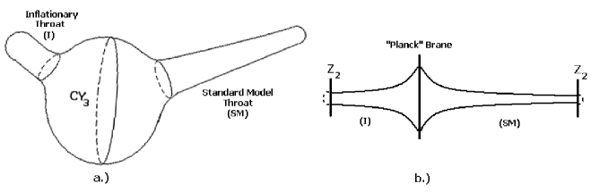
Figure 1: We will consider a KKLMMT setup with two throats, as in a.); as a simplification, we will consider the throats to be $AdS_{5}$, and glue the two throats together at a “Planck” brane, as in b.).

2 Setup

The setup is a Type IIB compactification on a Calabi-Yau (CY) 3-fold with NS-NS and R-R fluxes turned on along the internal compact dimensions. As in [16, 17], by turning on fluxes on the cycles associated with a conifold one can generate a strongly warped “throat” which is glued to the bulk CY compact space. The fluxes are quantized by:

$$\frac{1}{2\pi\alpha^{\prime}}\int_{A}F_{(3)} = 2\pi M$$

$$\frac{1}{2\pi\alpha^{\prime}}\int_{B}H_{(3)} = 2\pi K,$$ (2.1)

where $A$ and $B$ are the cycles on which the fluxes are supported. The throat is a warped deformed conifold where the deformation replaces the conifold singularity with an $S^{3}$ “cap”. Far from the tip of the throat the geometry looks like an exact conifold with 6-dimensional metric $ds^{2}_{6}=dr^{2}+r^{2}ds^{2}_{X_{5}}$. The 5-dimensional space $X_{5}$ is some Einstein-Sasaki manifold (e.g., $T^{1,1}$) whose details we will not be concerned with here.

Far from the deformation the throat can be described by the metric [24]:

$$ds^{2}=H^{-1/2}(r)g_{\mu\nu}dx^{\mu}dx^{\nu}+H^{1/2}(r)(dr^{2}+r^{2}ds^{2}_{X_{5}}),$$ (2.2)

where the warping is,

$$H(r)=\frac{1}{r^{4}}(R_{+}^{4}+R_{-}^{4}\log(\frac{r}{R_{+}})^{4}).$$ (2.3)

$R_{+}$ and $R_{-}$ are the radii of the $X_{5}$ at the top and bottom of the throat, respectively, and are given in terms of the flux quantizations as:

$$R_{+}^{4} = \frac{27\pi}{4}\ell_{s}^{4}g_{s}MK$$

$$R_{-}^{4} = \frac{3}{8\pi}\frac{27\pi}{4}\ell_{s}^{4}g_{s}^{2}M^{2}.$$ (2.4)

The throat geometry can be further simplified as $AdS_{5}\times X^{5}$ where $R_{+}\approx R$ is the $AdS$ curvature scale and the hierarchy between $R_{+}$ and $R_{-}$ sets the amount of warping in the throat $\frac{y_{0}}{R}\sim\frac{1}{4}\left(\frac{R_{+}}{R_{-}}\right)^{4}$, where the warp factor is approximately

$$h\equiv H^{-1/4}(r_{0})\approx\frac{r_{0}}{R_{+}}=e^{-y_{0}/R}=e^{-2\pi K/3Mg_{s}}.$$ (2.5)

Using the coordinate transformation $r/R=e^{-ky}$ ($k\equiv R^{-1}$) one can put the equation of motion for the metric flucuation $g_{\mu\nu}=\eta_{\mu\nu}+h^{(n)}_{\mu\nu}(x,y,\rho_{i})$ (where $\rho_{i}$ are the coordinates associated with the $X_{5}$) in the form [24] ($h^{(n)}_{\mu\nu}(x,y,\rho_{i})=e^{ip\cdot x}\chi^{(n)}(y)\Omega_{L}(\rho_{i})\epsilon_{\mu\nu}$, where $\epsilon_{\mu\nu}$ is the polarization):

$$(e^{4ky}\partial_{y}e^{-4ky}\partial_{y}+m^{2}e^{2ky}-k^{2}L^{2})\chi^{(n)}(y)=0,$$ (2.6)

where $m^{2}=p^{2}$ is the 4-D mass of the KK mode and $L^{2}$ is the quantized angular momentum on the $X_{5}$ whose structure we will leave unspecified. The solution of this equation is given by combinations of Bessel functions times an exponential:

$$\chi^{(n)}(y)=Ne^{2ky}[J_{\nu}(m_{n}Re^{ky})+BY_{\nu}(m_{n}Re^{ky})],$$ (2.7)

where $\nu^{2}=4+L^{2}$. (The bulk graviton zero mode is given as the limit as $m_{n}\rightarrow 0$). The quantization of the KK masses can be seen by imposing orbifold boundary conditions at the tip of the throat: $\partial_{y}\chi^{(n)}|_{y=y_{0}}=0$ implies that $J_{\nu-1}(m_{n}Re^{ky_{0}})=0$, so we find that the masses are quantized in units of the zeros of the Bessel function, $m_{n}\sim\frac{ne^{-ky_{0}}}{R}$ for mode numbers $n\gg\nu-1$ (more precisely, [24] find that KK modes localized near the bottom of the throat are quantized in units of the radius of the $S^{3}$ cap $m_{n}\sim\frac{ne^{-ky_{0}}}{R_{-}}$). Imposing continuity and jump boundary conditions across the Planck brane as in [41], we find $B\approx\frac{\pi}{8}\left(\frac{m_{n}}{k}\right)^{2}$.

The string scale is related to the 4-D Planck mass by $M_{Pl}^{2}=M_{s}^{8}V_{6}g_{s}^{-2}\epsilon^{2}$, where $V_{6}$ is the volume of the Calabi-Yau compactification, which we take to be slightly larger than $R_{+}^{6}$, and $\epsilon=\left(\frac{2}{(2\pi)^{7}}\right)^{1/2}$. Because $V_{6}\approx\beta R_{+}^{6}$ where $\beta$ is various factors of $2\pi$ from integrating out the extra dimensions in the conifold, we will take $V_{6}\epsilon^{2}\approx R_{+}^{6}$. In the paper we will be interested in staying within the SUGRA description where we can ignore trans-stringy excitations, thus we wish to have $R_{-}^{-1}<M_{s}$. We will parameterize the excess as $R_{-}M_{s}\approx R_{+}M_{s}/(\ln h_{i}^{-1})^{1/4}\approx\lambda(g_{s})^{1/4}/(\ln h_{i}^{-1})^{1/4}$, where $\lambda=(\frac{27\pi}{4}MK)^{1/4}$ and we wish to keep track of the explicit dependence on $g_{s}$. For deep enough throats almost all of the flux in the quantization conditions in Eq.(2.1) lies in the throats so one can have independent $AdS$ curvature scales for different throats, but for simplicity we will consider both throats to have the same $AdS$ scale, so the product $MK$ must be the same in both throats. (One can see that allowing the $AdS$ scales to differ gives us extra parameters to vary). We then have three parameters: $\lambda$ explained above, $h_{i}$ the warp factor of the I throat, and $h_{sm}$ the warp factor of the SM throat (we will take $g_{s}$ as fixed by requiring that $g_{s}\sim g_{YM}^{2}\sim\alpha$). These parameters can be further related by noting that the warp factor $h\equiv\frac{M}{M_{s}}$ gives the local string scale $M$ in the throat; because $M_{s}$ is related to $\lambda$ through the definintion of the Planck scale, $h_{i}$ and $h_{sm}$ have implicit $\lambda$ dependence as well. Making this dependence explicit,

$$h_{i} = \frac{M_{i}}{M_{Pl}}\frac{\lambda^{3}}{g_{s}^{1/4}}$$

$$h_{sm} = \frac{M_{sm}}{M_{Pl}}\frac{\lambda^{3}}{g_{s}^{1/4}}.$$ (2.8)

We will fix $M_{i}$ by requiring that the correct level of density perturbations $\frac{\delta\rho}{\rho}\sim\frac{H}{\epsilon M_{Pl}}$ is generated by the brane-antibrane potential (which is set by the local string scale in the inflationary throat). However, we will not commit ourselves to fixing the local string scale $M_{sm}$ at the tip of the Standard Model throat to be TeV scale during inflation. This will gives us more flexibility in satisfying the phenomenology of reheating and presumably other mechanisms can be used in conjunction with warping to generate the required hierarchy. Another possibility is that the Standard Model throat relaxes to its ground state after inflation [25] because generic arguments suggest that stringy corrections will tend to set $M_{sm}\sim H$ during the inflationary era, so a throat with a local string scale less than $H$ will generically become shorter during inflation after these corrections are taken into account.

3 Chain Processes

The reheating of the Standard Model is the last step of a sequence of processes that starts in the inflationary throat through $D\overline{D}$ annihilation and, through a chain of decays and tunneling, ends when the inflaton energy is transferred to the Standard Model degrees of freedom. The steps in the chain decay are:

• the transfer of energy from the tachyon to closed strings at the end of inflation (Section 3.1),

• the subsequent decay of closed strings into massless string states (Kaluza-Klein modes and gravitons) (Section 3.2),

• the interactions among these lower energy degrees of freedom (Section 3.3),

• the transfer of energy into the other throat(s) (via tunneling) (Section 3.4),

• the decay of these modes into Standard Model degrees of freedom and gravitons (Section 4).

Throughout these chain processes, one must consider various cosmological constraints in order to determine if a viable model of reheating can be constructed in a self-consistent way. For example, an overproduction of gravitons or the presence of relics could interfere with nucleosynthesis or overclose the universe and must be avoided. In the following we will analyze these issues systematically.

3.1 $D\overline{D}$ annihilation

The multi-throat scenario allows us to have a simple $D\overline{D}$ inflationary system in one throat and the Standard Model in a separate throat, sidestepping the problems of single throat inflation discussed in the introduction. Thus, the process of reheating is then more clearcut than a $DD\overline{D}$ system (single-throat model). The end of inflation is triggered by the condensation of the open string tachyon which develop when the distance between the brane-antibrane pair is sub-stringy, leading to what is known as the tachyon matter [37]. The latter can be thought of as a coarse-grained description of the actual physical state, a distribution of closed strings [36, 37, 38, 39]. By contrast, in the $DD\overline{D}$ case, the tachyon can couple directly to the open strings on the remaining (Standard Model) D-branes instead of the usual process of decaying into closed strings. The reheating process is then be more complicated and less understood (see, however, [24] for comments about the suppression of the coupling to the open string sector).

The properties of the annihilation process into closed strings (the spectrum, the energy density and its distribution) can presumably be captured by the decay of unstable D-branes: the tachyon matter is an (asymptotically) pressureless gas with energy momentum components only in the directions orthogonal to the D-branes [36, 37, 38, 39].

The total average number density and the total average energy density emitted were found in [38]:

$$\frac{\overline{N}}{V}=\sum_{s}\frac{1}{2E_{s}}|A_{s}|^{2}~{},\qquad\frac{\overline{E}}{V}=\sum_{s}\frac{1}{2}|A_{s}|^{2},$$ (3.1)

where $V$ is the volume of the branes, $A_{s}$ is the amplitude for producing a state $s$, $E_{s}=\sqrt{k^{2}+N}$ is its energy and $N$ is the oscillator level (note that we are taking $\alpha^{\prime}=4$).

For large $N$, $|A_{s}|^{2}\sim e^{-2\pi E_{s}}$ and the probability for every single state to be produced is

$$p_{s}=\frac{1}{2E_{s}}|A_{s}|^{2}\sim\frac{1}{\sqrt{k^{2}+N}}e^{-2\pi\sqrt{k^{2}+N}}.$$ (3.2)

Notice that it depends only on the level number $N$ and not on the partition of $N$ among the various oscillators forming the state, so every state at a given level $N$ is equally produced. Moreover, for fixed $N$ the probability is peaked on the states that have $\frac{k^{2}}{N}\sim 0$, i.e. the closed strings produced will predominately have no Kaluza-Klein modes or winding modes in the Calabi-Yau space.

Furthermore, for the energy density,

$$\frac{\overline{E}}{V}=\sum_{s}\frac{1}{2}|A_{s}|^{2}=\sum_{N}\int d^{d-3}k\ D(N)e^{-2\pi\sqrt{k^{2}+N}}\sim\sum_{N}\epsilon,$$ (3.3)

where $D(N)$ is the degeneracy of states at level $N$ and $\epsilon$ is independent of $N$, we see that the set of states at every level number $N$ receives the same amount of energy density. In other words, energy is equipartitioned among the oscillator levels labeled by $N$. If the maximum energy available for a single state is $\sim\frac{1}{g_{s}}$, then the maximum allowed level number is $N\sim\frac{1}{g_{s}^{2}}\sim 100$ if $g_{s}\sim.1$.

3.2 Decay of Closed Strings into KK modes

The next step in the energy conversion process is the decay of the closed strings into lighter degrees of freedom, namely the massless graviton and KK modes (see [24] for additional discussion). The Kaluza-Klein modes are localized deep inside the throat due to the warp factor, whereas the graviton has a non-zero wavefunction all over the Calabi-Yau. After proper normalization one finds that the KK mode wavefunctions are peaked deep in the throat by a factor of $h_{i}^{-1}$ relative to the graviton, so decay to the former is enhanced by a factor $h_{i}^{-2}$. However, decay to KK modes will be suppressed by phase space since the KK mass can be comparable to the local string scale, so it is not immediately clear whether KK modes or gravitons are preferred decay products.

We can estimate the decay rates into graviton and into Kaluza-Klein modes by an explicit (flat space) worldsheet computation. For a flat space computation to be valid the geometry must vary sufficiently slowly with respect to the string scale, i.e. for an AdS throat the AdS length must be less than the string length. However, since we require $R_{-}>\ell_{s}$ in order to use a SUGRA approximation, $R_{+}>R_{-}>\ell_{s}$, where $R_{+}$ is the AdS length, this condition is satisfied. The geometry induces a potential that localizes the string, and so the string effectively lives inside a box [30]. It must be stressed that since our calculation is for flat space it will not capture all of the features of decay in curved space; however, as an estimate we can compute the decay rates in flat space and convolve the results with the wavefunction square of the corresponding decay products, i.e., graviton and KK modes respectively, in order to take into account the enhancement of the KK mode wavefunction in the AdS space.

Let us compute the average decay rate for closed strings fixing: (i) the mass of the initial state ($M^{2}=N$), (ii) one of the final states (the graviton or the Kaluza-Klein mode), and (iii) the mass of the other final states ($M^{\prime 2}=N^{\prime}+p^{2}+k^{2}$). We do not fix, however, the specific initial state (over which we average) or final state, other than specifiying its mass level.

The decay is given by

$$\Gamma=g_{s}^{2}\int dP\sigma_{R}\ \sigma_{L}$$

where $d$ is the number of spatial dimensions, $\sigma_{R}$ is defined as

$$\sigma_{R}=\frac{1}{\mathcal{N}_{N_{R}}}\sum_{\Phi_{N}}\sum_{\Phi_{N^{\prime}}}\langle\Phi_{N}|V_{R}(k,1)^{\dagger}|\Phi_{N^{\prime}}\rangle\langle\Phi_{N^{\prime}}|V_{R}(k,1)|\Phi_{N}\rangle,$$

the vertex operator we need is $V=V_{R}V_{L}$, with

$$V_{R}(p,z)=c(z)e^{ip\cdot X_{R}(z)}(i\xi\cdot\partial X(z)+\frac{\alpha^{\prime}}{2}p\cdot\psi\xi\cdot\psi),$$

$\int dP$ is the integral over the phase-space and $\mathcal{N}_{N_{R}}$ is the number of states at level $N=N_{R}=N_{L}$.

In particular, as we saw in Section (3.1), the closed strings produced when the $D\overline{D}$ system decays have preferably momentum, Kaluza-Klein and winding charges equal to zero. The result of the computation (see, e.g., [42]) can be written in terms of $N$ and $N_{0}=N-N^{\prime}=2E\sqrt{N}$:

$$\cases{\Gamma_{g}\sim g_{s}^{2}\pi\Omega_{3}\left(\frac{N_{0}}{2\sqrt{N}}\right)^{3}{\frac{e^{-2a(\sqrt{N}-\sqrt{N-N_{0}})}}{\left(1-e^{-\frac{aN_{0}}{2\sqrt{N-N_{0}}}}\right)^{2}}}&for graviton\cr\Gamma_{KK}\sim g_{s}^{2}\pi\Omega_{3}\left(\frac{N_{0}}{2\sqrt{N}}\right)^{2}\frac{e^{-2a(\sqrt{N}-\sqrt{N-N_{0}})}}{\left(1-e^{-\frac{aN_{0}}{2\sqrt{N-N_{0}}}}\right)^{2}}\sum_{n=1}^{n_{max}}\sqrt{\frac{N_{0}^{2}}{4N}-k_{KK}^{(n)}}&for KK modes,\cr}$$ (3.4)

where $a=2\sqrt{2}\pi$, $\Omega_{3}$ is the angular integral in three dimensions, and $k_{KK}^{(n)}$ is the Kaluza-Klein momentum of the $n$-th KK mode. We have implicitly assumed that the KK mode has momentum only in the radial direction of the throat, although it is straightforward to include momenta in other directions of the Calabi-Yau as well. Note that in order to get these results we have approximated the distribution of states $D(N)$ by its limit for large $N$, but actually this approximation is already very good for moderate values of $N$.

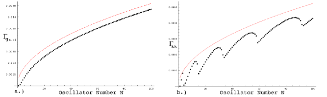
Figure 2: The numerical value of the decay rate (in units of the local string scale) of a closed string into an a.) graviton and b.) KK mode, for all allowed processes, is plotted for finite oscillator level $N$ (black dotted line), which is relevant for the decay of the closed string end products from $D\overline{D}$ annihilation, and in the limit $N\rightarrow\infty$ (red solid line), which corresponds to the field theory limit of [42], where $\Gamma\propto\sqrt{N}$ (note that we have not included any warp factor enhancement yet). The jumps in b.) are from threshold effects for the production of KK modes; see the discussion below Eq.(3.5).

To obtain the total decay rate into gravitons (or similarly KK modes) for any given initial state $N$, we sum over all the allowed processes labeled by $N_{0}$ where $N_{0}=1$ to $N$. Unlike [42], we have not taken $N\rightarrow\infty$ so the total decay rate into gravitons $\Gamma_{g}$ is valid for an initial state of finite mass. Recall that in the $N\rightarrow\infty$ limit, we can turn the sum over $N_{0}$ into an integral through the Jacobian $dN_{0}=2\sqrt{N}d\omega$, where $\omega=N_{0}/(2\sqrt{N})$,

$$\Gamma_{g,tot}\sim g_{s}^{2}\pi\Omega_{3}2\sqrt{N}\int_{0}^{\infty}d\omega\ \omega^{3}\frac{e^{-2a\omega}}{\left(1-e^{-a\omega}\right)^{2}}=c_{g}\sqrt{N},$$ (3.5)

where $c_{g}\approx 0.0018$. This corresponds to the field theory limit since as $N\rightarrow\infty$, the mass of the initial state $M\rightarrow\infty$ or equivalently $\alpha^{\prime}\rightarrow 0$. As can be seen from Figure 2, taking finite $N$ gives a smaller value for $\Gamma_{g,total}$ than would be expected from field theory, however the parametric dependence of $\Gamma_{g}(N)\propto\sqrt{N}$ as discussed in [42] is unchanged. The difference between the two curves in Figure 2 is due to the stringy corrections to the decay rate, namely that decays must occur in discrete steps of energy. One can obtain similar looking expressions for the KK modes, where once again the parametric dependence on $N$ is $\Gamma_{KK}(N)\approx c_{KK}\sqrt{N}$, where $c_{KK}\approx 0.0002$ without the warp factor. The finite $N$ solution shows some qualitatively different features than the limiting case: the jumps are produced when, for fixed $N_{0}$, $N$ becomes large enough that a KK mode cannot be produced, i.e. $n_{max}<1$. In particular, the jump at $N=15$ is for $N_{0}=2$ (where $\lambda\sim 5$ and $g_{s}\sim.1$, which as we will see below are reasonable values): above $N=15$ one cannot produce a KK mode with $N_{0}=2$, so we drop below threshold. There are multiple jumps because we are summing over all $N_{0}$, so we pick up multiple threshold effects. Notice how this is different from the $N\rightarrow\infty$ limit, where we only obtain the enveloping behavior.

The sum over the mode number $n$ of the KK modes of the square root in Eq.(3.4) is the phase space available to the decay when the KK mode has a non-zero 4D mass, and the sum is over all kinematically allowed KK modes. Notice that for small $N_{0}$ the energy released by the decay is also small so it is difficult to produce KK modes, and the phase space factor reduces the rate of decay into KK modes. For large $N_{0}$, i.e. $N_{0}\sim N$, more KK modes can be produced, however the decay rate then depends exponentially on $\sqrt{N}$ and is highly suppressed. The phase space factor and the exponential suppression of decay with large $N_{0}$ compete to maximize the decay rate into KK modes for fixed $N$ for $N_{0,max}^{KK}\sim a_{KK}\sqrt{N}$, where one can numerically determine $a_{KK}\sim.65$, so we see that only low lying KK modes ($n_{max}\sim\frac{.65\lambda g_{s}^{1/4}}{(\ln h_{i}^{-1})}$) are produced. Similarly, one can determine that gravitons are produced most often for $N_{0,max}^{g}\sim a_{g}\sqrt{N}$, $a_{g}\approx\frac{3}{2a}$.

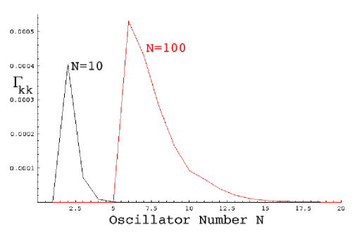
Figure 3: The numerical value of the decay rate of a $N=100$ (red) and $N=10$ (black) closed string into a KK mode for different decay processes $N_{0}=N-N^{\prime}$. Notice that the decay rate is peaked at small $N_{0}$ and falls off quickly, but increasing $N$ increases the $N_{0}$ at which the rate is maximum. The large initial jump when $N_{0}\approx N_{0,max}$ is due to the decay process crossing the threshold for production of a KK mode. One can show that $N_{0,max}\sim.65\sqrt{N}$.

Without any enhancement from the warp factor we find that $\Gamma_{g}(N)/\Gamma_{KK}(N)\sim c_{g}/c_{KK}\sim.1$ over $N=1$ to $100$, and so we see that a warp factor enhancement may help in making KK modes a preferred decay product; however, the order of magnitude of the KK decay rate is strongly dependent on the size of the $S^{3}$ cap $R_{-}$ because this determines how easily a KK mode can be produced. Changing the value by a small amount leads to large variations in the decay rate, e.g. changing $R_{-}$ by a factor of 5 can modify the KK decay rate by $\sim 7$ orders of magnitude ($c_{KK}\rightarrow 10^{-11}$)!

What we are really interested in, however, is the ratio of the total amount of energy deposited into KK modes versus gravitons. This can be estimated through the following argument. The typical time for an initial state $N_{in}$ to decay into either a graviton or KK mode is:

$$\Delta t_{N_{in}}\sim\frac{\Delta N}{\sum_{N_{0}=1}^{N_{in}}\Gamma_{g}(N_{in},N_{0})N_{0}+\Gamma_{KK}(N_{in},N_{0})N_{0}},$$ (3.6)

where $\Delta N\sim a_{p}\sqrt{N}$ is the typical step size. We will take $a_{p}\sim a_{KK}$ if the KK modes have a larger decay rate and $a_{p}\sim a_{g}$ otherwise. The total number of species $i=\{\mbox{graviton, KK}\}$ produced by a closed string $N_{in}$ is then,

$${\cal N}_{N_{in}}^{i}=\sum_{N=1}^{N_{in}}\left(\sum_{N_{0}}\Gamma_{i}(N,N_{0})\right)\Delta t_{N}\sim\sum_{N=1}^{N_{in}}\frac{a_{p}c_{i}}{a_{g}c_{g}+a_{KK}c_{KK}},$$ (3.7)

where we have approximated $\sum_{N_{0}}\Gamma_{i}(N,N_{0})\sim c_{i}\sqrt{N}$ and $N_{0,max}^{i}\sim a_{i}\sqrt{N}$. The total number of species produced by the closed strings is then the weighted sum over all oscillator levels:

$${\cal N}_{tot}^{i}=\sum_{N_{in}=1}^{g_{s}^{-2}}\sum_{s}p_{s}(N_{in}){\cal N}_{N_{in}}^{i}=\sum_{N_{in}=1}^{g_{s}^{-2}}\sum_{N=1}^{N_{in}}\frac{a_{p}c_{i}}{(a_{g}c_{g}+a_{KK}c_{KK})\sqrt{N}};$$ (3.8)

similarly, the fraction of energy carried by species $i$ is

$$E_{i}\sim\sum_{N_{in}=1}^{g_{s}^{-2}}\sum_{s}p_{s}(N_{in}){\cal N}_{N_{in}}^{i}\frac{N_{0,max}}{2\sqrt{N}}\sim\sum_{N_{in}=1}^{g_{s}^{-2}}\sum_{N=1}^{N_{in}}\frac{a_{p}a_{i}c_{i}}{(a_{g}c_{g}+a_{KK}c_{KK})2\sqrt{N}}.$$ (3.9)

We see then that the fraction of energy carried by KK modes versus gravitons is $E_{KK}/E_{g}\sim a_{KK}c_{KK}/(a_{g}c_{g})\approx 0.2h_{i}^{-2}$, so even for mildly warped throats $h_{i}\sim 10^{-2}$ we see that the KK modes appear to be preferred decay products.

One can estimate the total time for the decay of the closed strings into KK modes and gravitons by considering the decay time for the most massive closed string. In this case, the total time for decay is the sum of each of the steps,

$$\Delta t_{tot}\sim\sum_{N=1}^{g_{s}^{-2}}\Delta t_{N}=\sum_{N=1}^{g_{s}^{-2}}\frac{a_{p}}{(a_{g}c_{g}+a_{KK}c_{KK})\sqrt{N}}.$$ (3.10)

For the case where gravitons dominate, $a_{g}c_{g}\gg a_{KK}c_{KK}$, we have $\Delta t_{tot}\sim\frac{1}{c_{g}}\sum_{N=1}^{g_{s}^{-2}}\frac{1}{\sqrt{N}}$ $\sim 5\times 10^{3}\sqrt{\alpha_{i}^{\prime}}$, while for the case where the KK modes are dominant decay products due to the warp factor enhancement, $\Delta t_{tot}\sim\frac{1}{c_{KK}}\sum_{N=1}^{g_{s}^{-2}}\frac{1}{\sqrt{N}}=5\times 10^{4}\sqrt{\alpha_{i}^{\prime}}$.

3.3 KK mode interactions

Because the KK modes carry conserved quantum numbers they cannot decay into lighter degrees of freedom unless they collide with another KK mode with opposite quantum number in the throat. The time scale of such collisions is found by estimating when the average number of collisions (the number density of the particle times the column depth times the cross-section of interaction) is approximately one, i.e. $\tau\sim(n\sigma v)^{-1}$, where $n$ is the particle number density, $\sigma$ is the cross-section, and $v$ is the velocity. The KK modes as initial decay products of excited closed strings are relativistic. This can be seen as follows. The average energy per KK mode is approximated by the average energy per closed string

$$\bar{E}_{KK}\sim M_{s}h_{i}=M_{i}$$ (3.11)

and their mass is

$$m_{KK}\sim\frac{h_{i}}{R_{-}}$$ (3.12)

therefore $\frac{\bar{E}_{KK}}{m_{KK}}\sim\frac{R_{-}}{\sqrt{\alpha^{\prime}}}$ and so we can assume $v\sim 1$ (taking $v<1$ will only increase the annihilation time). Moreover, as we will see, the KK modes thermalize quickly so it is reasonable to take $v\sim 1$ in estimating the time scales for the processes involved in the inflationary throat. The KK states can annihilate and pair produce gravitons or other (kinematically allowed) KK modes. The cross-section for KK modes to annhilate into bulk gravitons is set by the Planck scale $\sigma\sim M_{Pl}^{-2}$. We will approximate the number density after inflation by the total energy density after inflation divided by the average energy per KK mode; the energy density after inflation is,

$$\epsilon_{I}=2T_{3}h_{i}^{4}\sim\frac{(M_{s}h_{i})^{4}}{g_{s}}=\frac{M_{i}^{4}}{g_{s}},$$ (3.13)

where $T_{3}$ is the tension of a $D3$. The average energy per KK mode is, as we said above, (3.11). The number density after inflation then is given by $n_{I}\sim\frac{M_{i}^{3}}{g_{s}}$. Plugging these values in we can obtain a rough estimate for the timescale for KK modes to decay to gravitons:

$$\tau_{g_{\mu\nu}}\sim g_{s}\left(\frac{M_{Pl}}{M_{i}}\right)^{2}\frac{1}{M_{i}}.$$ (3.14)

As mentioned above, KK modes can interact among themselves and thermalize, coming to a thermal temperature $T_{KK}$ (see also [24]). The timescale for thermalization is similar to the timescale for KK modes to interact and decay to gravitons, except that the cross-section is now set by the local scale, $\sigma\sim g_{s}^{2}(M_{s}h_{i})^{-2}=g_{s}^{2}M_{i}^{-2}$. We immediately see, then, that the timescale for thermalization of the KK modes is much smaller than the timescale for KK modes to decay into gravitons:

$$\tau_{thermal}\sim\frac{1}{g_{s}M_{i}}.$$ (3.15)

We can estimate the thermal temperature of the relativistic KK modes by setting the thermal energy density equal to the initial energy density of the $D\overline{D}$ system:

$$\epsilon_{therm}=g_{KK}T^{4}_{KK}=\epsilon_{I}\sim\frac{(M_{i})^{4}}{g_{s}}.$$ (3.16)

The number of KK degrees of freedom $g_{KK}$ is approximately equal to the number of relativistic KK modes, as we will argue below. The temperature of the KK modes, then, is:

$$T_{KK}\sim\frac{M_{i}}{(g_{KK}g_{s})^{1/4}}.$$ (3.17)

Since only KK states with $m_{n}<T_{KK}$ are relativistic, we see that only states with mode numbers $i\leq i_{rel}\sim(\frac{\lambda}{(\ln h_{i}^{-1})^{1/4}})^{4/5}$ are relativistic; since the number density of non-relativistic modes has an $e^{-m/T}$ suppression, most KK modes will occupy relativistic degrees of freedom, thus $g_{KK}\approx i_{rel}$. Note that the actual low-lying zeros of the Bessel functions of order 2 do not follow the simple relation $m_{n}\sim n\frac{h_{i}}{R}$, but instead are at a higher mass level than this relation would suggest. As we will see below we expect $\lambda$ to be small, thus $i_{rel}$ will also be small, so only the very lowest lying KK states will be excited. Since angular states, as discussed in [24], are zeros of Bessel functions of a larger order $\nu^{2}=4+L^{2}$ where $L$ is a conserved quantum number of the internal space, the lowest lying angular KK modes will be above the small thermal temperature and thus we do not expect that they will be present in significant numbers after thermalization.

3.4 KK tunneling

We would now like to estimate the time required for modes localized in the I throat to tunnel into the SM throat. One can consider a toy model of the two throat system by gluing two finite RS spaces together at the Planck brane as in [41, 23] (see Figure 4). Under the coordinate transformation $z+R=Re^{ky}$, the metric can also be written in the form,

$$ds^{2}=\frac{R^{2}}{(|z|+R)^{2}}(\eta_{\mu\nu}dx^{\mu}dx^{\nu}+dz^{2}),$$ (3.18)

where $R=R_{+}$ as before is the $AdS$ curvature scale. We will place the IR brane for the inflationary throat at $z=-z_{i}\approx-Rh_{i}^{-1}$ and the IR brane for the SM throat at $z=z_{sm}\approx Rh_{sm}^{-1}$. The utility of expressing the metric in these coordinates is that the equation of motion for the KK modes of the graviton,

$$h_{\mu\nu}(x,z)=\sqrt{\frac{R}{|z|+R}}e^{ip\cdot x}\psi_{\mu\nu}(z),$$ (3.19)

becomes a simple Schrödinger equation for $\psi$ (suppressing the indicies):

$$\partial_{z}^{2}\psi(z)+(m^{2}-\frac{15}{4(|z|+R)^{2}})\psi(z)=0,$$ (3.20)

where the potential felt by the KK mode $V(z)=\frac{15}{4(|z|+R)^{2}}$ is proportional to the square of the warp factor (we have ignored the extra part of the potential felt by the angular states).

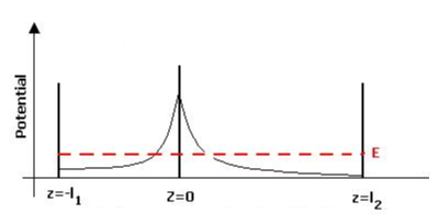
Figure 4: The warping creates a potential barrier for Kaluza-Klein states of the graviton in the Schrödinger coordinate system. States initially localized in the inflationary (left) throat must tunnel through this barrier to communicate with the Standard Model (right) throat. The Schrödinger energy of a state is $E=m^{2}$.

The general solution to this equation of motion can be expressed in terms of Bessel functions,

$$\psi(z)=\sqrt{m(|z|+R)}[AJ_{2}(m(|z|+R))+BY_{2}(m(|z|+R))].$$ (3.21)

We impose $\mathbb{Z}_{2}$ boundary conditions at the IR branes (which gives us our mass gap as discussed in Section 2) and the appropriate Israel jump conditions at the Planck brane. We would like to consider tunneling of an incoming state from the left hand throat into a state on the right hand throat for which [41] finds a tunneling probability for $m_{n}R\ll 1$ (certainly the case after thermalization for mode number $n\lesssim h_{i}^{-1}\sim 10^{4}$) of

$$P\sim(m_{n}R)^{4}.$$ (3.22)

In the calculation of [41] the reflection of the KK mode at the wall of the finite SM throat was not included, and one may worry that this reflection may significantly alter the tunneling results. However, one can see that the $\mathbb{Z}_{2}$ reflection will only increase the amplitude in the SM throat by a factor of 2 (i.e. constructive interference), and when it tunnels back through the barrier will contribute a vanishingly small amount to the I throat. Performing the calculation explicitly by including the reflected wave confirms this conclusion (see Appendix A), namely that the probability Eq.(3.22) is effectively unchanged.

The tunneling rate from throat I to throat SM is found by multiplying the tunneling probability Eq.(3.22) by the flux, the inverse of the potential wall length $\frac{1}{|z_{i}|}$, so the tunneling rate from throat I to throat SM is:

$$\Gamma_{tunn}\sim(mR)^{4}\frac{1}{|z_{i}|}.$$ (3.23)

Note that when a KK mode tunnels from throat I to throat SM the mass $m$ of the mode stays (approximately) the same, and since the $AdS$ lengths are the same, the tunneling probability back to the I throat is the same (making the $AdS$ lengths different will make the tunneling probability more asymetrical, suppressing the tunneling more in one direction than the other). The tunneling rate, however, is inversely proportional to the (conformal) length of the throat, thus modes in a long throat take longer to tunnel out. Note that the depth of the two wells is approximately the same and does not cause much difference in the tunneling rates. This can be understood semi-classically as follows. The average time required for a particle to escape a potential well is the average number of collisions required to escape multiplied by the time between collisions. The average number of collisions required is the inverse of the tunneling probability, $P^{-1}$. The time required is twice the length of the well divided by the speed of the particle. In conformal coordinates, Eq.(3.18), the KK modes behave like massless Klein-Gordon particles, and the length of the potential well is measured in terms of the conformal length, thus the average time required for a KK mode to escape is $\tau_{tunn}\sim P^{-1}2|z_{i}|$, which gives the tunneling rate Eq.(3.23) (up to a factor of two).

The tunneling rate can also be represented as the mixing between two weakly coupled potential wells, as in [24]:

$$\Gamma=|\langle SM|e^{-iH\Delta t}|I\rangle|^{2}\cdot\mbox{Flux},$$ (3.24)

where

$$H=\left(\begin{array}[]{cc}m&\epsilon\\ \epsilon&m^{\prime}\end{array}\right)$$ (3.25)

is the Hamiltonian for the coupled system, $\Delta m=|m-m^{\prime}|$, and $\epsilon$ is the coupling of the systems. Note that $\Delta m$ is the difference in mass between states in the two throats, not the mass gap within the throats. To leading order in $\epsilon$ one finds,

$$\Gamma\approx\frac{\epsilon^{2}}{\Delta m^{2}}\cdot\mbox{Flux}.$$ (3.26)

The coupling of the two systems $\epsilon$ should be proportional to some power of the tunneling probability; [24] suggests that $\epsilon\sim m(mR_{-})^{2}$, which seems to imply $\Gamma\sim\frac{m^{2}}{\Delta m^{2}}(mR_{-})^{4}\cdot\mbox{Flux}$; in order to get Eq.(3.23) we must have $m\sim\Delta m$. But this says that the difference in mass between the states in different wells is proportional to the mass level, which seems unlikely in a general setup. Instead, one can show that for a symmetric double well, the expression for $\epsilon$ should be $\epsilon\sim\Delta m(mR_{-})^{2}$ (note that the flux is still $z_{i}^{-1}$). This makes sense, since the coupling between two weakly coupled potential wells should be proportional to the splitting of their adjacent masses.

A crucial aspect (as noted in [23]) of the viability of warped reheating is the ability to channel energy into Standard Model degrees of freedom and not to lose energy to bulk gravitons, which can ruin BBN and other cosmological observations. Naively one would expect the perturbative decay of KK modes to gravitons to dominate over the non-perturbative tunneling effects, thus reheating would fail to channel energy onto the Standard Model branes effectively. However, several effects seem to render this intuition invalid. First, as noted above, the warping induces small couplings between the gravitons and KK modes. Second, KK to graviton decay must occur via pair annihilation in order to conserve extra dimensional quantum numbers, so the decay can only happen when a KK mode finds its partner with opposite quantum numbers. Because of these effects, it is possible that there exists a range of parameters for the model for with $\frac{\tau_{tunn}}{\tau_{g_{\mu\nu}}}\lesssim 1$. Since thermalization drops the KK states down to the lowest mass levels, we will take $m\sim h_{i}/R_{-}$, which is the longest timescale for tunneling. We find,

$$\frac{\tau_{tunnel}}{\tau_{g_{\mu\nu}}}\sim\frac{g_{s}^{1/4}}{\lambda^{11}}\left(\frac{M_{Pl}}{M_{i}}\right)^{2}.$$ (3.27)

We find that for,

$$\lambda\geq\left(\left(\frac{M_{Pl}}{M_{i}}\right)^{2}g_{s}^{1/4}\right)^{1/11},$$ (3.28)

one can suppress the decay to gravitons. For $M_{i}/M_{Pl}\sim 10^{-4}$ and $g_{s}\sim.1$ this gives a lower limit $\lambda\geq 5$, and keeps $R_{-}>\ell_{s}$, which is what we wanted in order to trust the SUGRA approximation anyway. However, this sets $h_{i}\sim 10^{-2}$, so the “throat” is not very strongly warped, which also helps the modes tunnel through.

An important question is whether the tunneling takes place within the Hubble time after inflation, for otherwise the tunneling does not take place until the Hubble rate falls below the tunneling rate (which has implications for KK interactions in the SM throat). The Hubble time after inflation is found from $H_{I}^{2}=\frac{1}{M_{Pl}^{2}}\epsilon_{0}$, and so the ratio of the tunneling time to the Hubble time is,

$$\frac{\tau_{tunnel}}{H_{I}^{-1}}\sim\frac{g_{s}^{3/4}}{\lambda^{11}}\left(\frac{M_{Pl}}{M_{i}}\right)^{3}.$$ (3.29)

Thus, for $\lambda\lesssim\left(\left(\frac{M_{Pl}}{M_{i}}\right)^{3}g_{s}^{3/4}\right)^{1/11}\sim 10$ we must consider Hubble expansion for tunneling. Note that while this gives us a small range of $\lambda$, this small range already implicitly existed since $h_{i}\propto\lambda^{3}$ and we want $h_{i}<e^{-1}$ for a warped throat, thus too large of $\lambda$ ruins the warping of the throat. One can also check that the KK modes thermalize within a Hubble time for $g_{s}\geq(M_{Pl}/M_{i})^{2}\sim 10^{-8}$ and so for $\lambda$ within the values $\left(\left(\frac{M_{Pl}}{M_{i}}\right)^{2}g_{s}^{1/4}\right)^{1/11}\lesssim\lambda\lesssim\left(\left(\frac{M_{Pl}}{M_{i}}\right)^{3}g_{s}^{3/4}\right)^{1/11}$ ($5\lesssim\lambda\lesssim 10$), corresponding to $1.9~{}\ell_{s}\lesssim R_{-}\lesssim 4.5~{}\ell_{s}$ (which are within our approximation $R_{-}>\ell_{s}$), we have the hierarchy of timescales: $\tau_{therm}\ll H_{I}^{-1}\lesssim\tau_{tunnel}\lesssim\tau_{g_{\mu\nu}}$.

4 Standard Model Throat

After the KK modes from the I throat tunnel into KK modes in the SM throat these KK modes can do several things in the SM throat, each with its own timescale: 1) decay to gravitons $\Delta t_{g_{\mu\nu}}$, 2) decay to Standard Model degrees of freedom $\Delta t_{SM}$, 3) tunnel out of the SM throat $\Delta t_{tunnel}$ and 4) thermalize and drop down to relativistic degrees of freedom at the bottom of the throat $\Delta t_{therm}$, all of which can happen relative to 5) the Hubble timescale $H_{tunn}^{-1}$.

Before we determine any of these timescales, we must determine the approximate number density of the KK modes after tunneling, which will be important in our calculation of the thermalization and graviton decay timescales. Since the number density falls off as $a(t)^{-3}$, where $a(t)$ is the scale factor, the number density after tunneling is,

$$n_{tunn}\sim n_{I}\left(\frac{a_{I}}{a_{tunn}}\right)^{3},$$ (4.1)

We will estimate the energy density for the modes to be non-relativistic, which falls off as $a^{-3}$, and since the tunneling will happen after the Hubble rate drops below the tunneling rate, i.e. $H^{2}_{tunn}\sim\frac{1}{\tau_{tunn}^{2}}\sim\frac{1}{M_{Pl}^{2}}\epsilon_{tunn}$ we have:

$$\epsilon_{tunn}\sim\frac{M_{Pl}^{2}}{\tau_{tunn}^{2}}\sim\epsilon_{I}\left(\frac{a_{I}}{a_{tunn}}\right)^{3}.$$ (4.2)

Putting Eqs.(4.1)(4.2) together we find

$$n_{tunn}\sim n_{I}\left(\frac{H_{I}^{-1}}{\tau_{tunn}}\right)^{2}\sim\frac{M_{i}^{3}}{g_{s}}\left(\frac{H_{I}^{-1}}{\tau_{tunn}}\right)^{2}.$$ (4.3)

We can now use this to estimate the thermalization and graviton decay time scales for the KK modes in the SM throat as in Section 3.

4.1 KK graviton decay

We again estimate the decay of KK modes to gravitons as $\Delta t_{g_{\mu\nu}}\sim(n\sigma v)^{-1}$, where we will take $v\sim 1$ and $\sigma\sim M_{Pl}^{-2}$ as before. For the number density we will use the estimate Eq.(4.3) after tunneling, and our estimate for the graviton decay timescale is then

$$\Delta t_{g_{\mu\nu}}\sim\left(\frac{M_{Pl}}{M_{i}}\right)^{2}\left(\frac{\tau_{tunn}}{H_{I}^{-1}}\right)^{2}\frac{g_{s}}{M_{i}}.$$ (4.4)

Similarly, we estimate the timescale for thermalization $\Delta t_{therm}$ of the KK modes where we note that now the cross-section is suppressed only by the local string scale in the SM throat, $\sigma\sim g_{s}^{2}(M_{s}h_{sm})^{-2}=g_{s}^{2}M_{sm}^{-2}$, so that the thermalization time scale is again much faster than the decay to gravitons, and is given by:

$$\Delta t_{therm}\sim\left(\frac{M_{sm}}{M_{i}}\right)^{2}\left(\frac{\tau_{tunn}}{H_{I}^{-1}}\right)^{2}\frac{1}{g_{s}M_{i}}.$$ (4.5)

4.2 Decay to Standard Model degrees of freedom

The decay rate of KK particles to Standard model degrees of freedom on a brane located at $y=y_{0}$ in the throat can be estimated by considering the interaction to be of the form [43, 44, 45] (where we are considering only the $AdS_{5}$ part of the throat here):

$${\cal L}_{int}\sim-\frac{1}{M_{Pl,5}^{3/2}}T^{\mu\nu}(x)h_{\mu\nu}(x,y_{0}),$$ (4.6)

where $M_{Pl,5}$ is the 5-D Planck mass, related to the 4-D Planck mass by $M_{Pl}^{2}=M_{Pl,5}^{3}R(1-h_{sm})\approx M_{Pl,5}^{3}R$, and $T^{\mu\nu}(x)$ is the energy-momentum tensor of the Standard Model fields. The metric flucuation $h_{\mu\nu}(x,y)$ can be expanded as:

$$h_{\mu\nu}(x,y)=\sum_{n=0}^{\infty}h_{\mu\nu}^{(n)}(x)\frac{\psi^{(n)}(y)}{\sqrt{R}}.$$ (4.7)

The 5-D part of the wavefunction $\psi^{(n)}(y)$ is given by the general formula Eq.(3.21) and is normalized as $\int dye^{y/R}\psi^{(m)}(y)\psi^{(n)}(y)=\delta_{nm}$. Using the normalization, the expansion of the KK modes Eq.(4.7), and the definition of the 5-D Planck mass we have then,

$${\cal L}_{int}=-\frac{1}{M_{Pl}}T^{\mu\nu}(x)h^{(0)}_{\mu\nu}(x)-\frac{1}{h_{sm}M_{Pl}}T^{\mu\nu}(x)\sum_{n=1}^{\infty}h^{(n)}_{\mu\nu}(x),$$ (4.8)

where $h_{sm}$ is set by the local string scale $M_{sm}$ at the tip of the Standard Model throat.

The decay rate to Standard Model fields is then approximately [44]:

$$\Gamma_{SM}\sim m_{KK}^{3}\frac{1}{M_{sm}^{2}}.$$ (4.9)

A more precise determination of the decay rate, including loop corrections, can be found in [43, 44, 45, 46], where we have ignored the extra contributions which depend on the ratio of the mass of the Standard Model particles and the mass of the KK modes, $m_{sm}/m_{KK}\ll 1$. Note that this estimate is similar to that of [24], where they consider decay of KK modes into the scalar transverse excitations of the brane [46] which then quickly decay into Standard Model degrees of freedom:

$$\Gamma_{KK}\sim m_{KK}^{3}\frac{\sqrt{1-\frac{4\mu^{2}}{m_{KK}^{2}}}}{M_{sm}^{2}}.$$ (4.10)

Here $\mu$ is the effective mass of the $\overline{D3}$ ($D3$) induced by the background fluxes (SUSY breaking). We see that for $\mu\ll m_{KK}$ we can neglect the square root in Eq.(4.10) and this decay rate is similar to the decay to Standard Model particles. However, since $m_{KK}\sim h_{sm}R_{-}^{-1}$ and a $\overline{D3}$ will have $\mu\sim h_{sm}/R_{-}$ from the fluxes, the decay rate to the transverse fluctuations becomes effectively zero. Decays directly to Standard Model degrees of freedom thus have more phase space and we will use Eq.(4.9) to determine the decay time to Standard Model degrees of freedom. Using $m\sim h_{sm}R_{-}^{-1}$ we find,

$$\Delta t_{SM}\sim\frac{\lambda^{3}g_{s}^{3/4}}{M_{sm}(\ln h_{sm}^{-1})^{3/4}}$$ (4.11)

4.3 Reheating

We would like the decay of KK modes into Standard Model particles Eq.(4.11) to be quicker than the decay into gravitons Eq.(4.4),

$$\frac{\Delta t_{sm}}{\Delta t_{g_{\mu\nu}}}\sim\lambda^{25}\left(\frac{M_{i}}{M_{Pl}}\right)^{8}\frac{M_{i}}{M_{sm}}\frac{(\ln h_{i}^{-1})^{1/2}}{g_{s}^{7/4}(\ln h_{sm}^{-1})^{3/4}}.$$ (4.12)

We find that for $M_{sm}\sim M_{i}$, this ratio is less than one for the range of $\lambda$ quoted at the end of Section 3, thus the decay to Standard Model degrees of freedom is favored. However, for $M_{sm}/M_{i}\sim 10^{-11}$ (i.e. $M_{sm}\sim$ Tev if one wants to generate the weak scale hierarchy during inflation) we must bring $\lambda$ down to such small values in order to have this process be favored that it does not appear we can simultaneously ensure that the KK modes in the inflationary throat tunnel and the KK modes in the SM throat reheat the Standard Model degrees of freedom. This can be seen by noting that less massive modes couple weaker to Standard Model degrees of freedom, Eq.(4.9). A deeper throat means that the lightest KK modes in the throat are less massive, thus couple weaker to the Standard Model. Meanwhile $\Delta t_{g_{\mu\nu}}$ is insensitive to the details of the throat construction, so eventually KK to graviton decay is favored.

The ratio of the time to decay to Standard Model particles and the Hubble time is,

$$\frac{\Delta t_{SM}}{H_{tunn}^{-1}}\frac{M_{i}}{M_{sm}}\left(\frac{M_{i}}{M_{Pl}}\right)^{4}\frac{1}{(\ln h_{sm}^{-1})^{1/4}}\frac{\lambda^{14}}{g_{s}^{1/2}}$$ (4.13)

This ratio is less than one for $M_{i}\sim M_{sm}$ as we took above and for all $\lambda$ in the range quoted above at the end of Section 3. Thus, we expect that the reheating of the Standard Model from KK modes decaying in the Standard Model throat will take place immediately after those modes tunnel. Also note that $\Delta t_{sm}<H_{I}^{-1}\approx\tau_{tunn}\leq\Delta t_{tunn}$, with the last inequality saturated for $M_{i}\sim M_{sm}$, so the modes will not tunnel back out before decaying to the Standard Model. One can also check that the ratio of the thermal time to the Hubble scale after tunneling is,

$$\frac{\Delta t_{therm}}{H_{tunn}^{-1}}\approx\left(\frac{M_{sm}}{M_{i}}\right)^{2}\left(\frac{M_{Pl}}{M_{i}}\right)^{2}\frac{1}{\lambda^{7}g_{s}^{3/4}},$$ (4.14)

which is greater than one for $M_{sm}\sim M_{i}$ and the appropriate ranges of $\lambda$. Thus, the KK modes are no longer thermal once they tunnel into the Standard Model throat.

Because the decay of the KK modes in the Standard Model throat is very quick, reheating happens when the Hubble rate drops below the tunneling rate, Eq.(3.23); when this happens the Standard Model brane is reheated and the energy density is

$$\epsilon_{RH}\sim g_{*}T_{RH}^{4}\sim M_{Pl}^{2}H_{tunn}^{2}\sim\frac{M_{Pl}^{2}}{\tau_{tunn}^{2}}.$$ (4.15)

Here $g_{*}\sim 100$ is the number of Standard Model degrees of freedom, and solving for the reheating temperature we obtain:

$$T_{RH}\sim\frac{M_{i}}{g_{*}^{1/4}}\left(\frac{M_{i}}{M_{Pl}}\right)^{3/2}\left[\frac{\lambda^{11}}{g_{s}^{5/4}}\right]^{1/2}.$$ (4.16)

For $M_{i}\sim M_{sm}$ and the range of values of $\lambda$ for which the reheating process seems to efficiently channel energy onto the Standard Model brane, i.e. for the tunneling out of the I throat to be quicker than decay into gravitons and for the decay to Standard Model particles to be faster than the decay to gravitons in the SM throat we have the range of reheating temperatures $10^{13}GeV\leq T_{RH}\leq 10^{14}GeV$. Notice that this range of values is smaller than $M_{sm}\sim 10^{15}GeV$, which implies that the KK modes do not excite stringy degrees of freedom, and we can trust this field-theory description of reheating. Note also that larger values of $\lambda$ could push the reheat temperature above $M_{i}$, but then we would have little to no warping for the inflationary throat (see Eq.(2.8)).

5 Adding More Throats

In a scenario with multiple (more than two) throats there are additional concerns that must be addressed: How are the tunneling KK modes from the I throat partitioned between the throats? Will KK modes from other throats decay to gravitons or decay to Standard Model particles at late times, ruining BBN?

To address the first question, notice that Eq.(3.23) for the tunneling rate of KK modes from the I throat does not depend at all on the details of the SM throat. One can make this more explicit by writing the mass as $m_{n}\sim\frac{nh_{i}}{R_{-}}$ and $z_{i}\sim R_{+}h_{i}^{-1}$: $\Gamma_{tunn}\sim n^{4}h_{i}^{5}/R_{+}$. Thus we expect that each throat will receive equal amounts of KK modes from the tunneling process. A similar conclusion was found in [24] by modifying the earlier discussion of the tunneling rate in Section 3, using the Hamiltonian. However, the 4-D mass of the KK modes is conserved (actually, it may be broken by the gluing of the throat to the CY 3-fold bulk or the presence of D-branes, but this breaking should be further suppressed) so a KK mode of mass $m_{n}\sim\frac{nh_{i}}{R_{-}}$ in the I throat can only decay into a mode with mass $m_{n}\approx m_{n^{\prime}}\sim\frac{n^{\prime}h_{X}}{R_{-}}$ in another throat with warp factor $h_{X}$. For a long throat like the SM throat the mass spacing $\Delta m\sim\frac{h_{sm}}{R_{-}}$ is small so it is more likely for a tunneling mode to find a (nearly) equal mass in this throat than in less-warped throats (this is also true for modes tunneling from a throat other than I). However, it has been suggested that stringy corrections will shorten a long throat to be approximately the same length as the inflationary throat (more precisely, the length is set by the Hubble scale during inflation) [25]; in this case the lengths of all throats will be approximately the same, and the KK modes will again be able to find equal mass states to tunnel into.

If there are other throats with the same length as the I throat (modified in the same way due to string corrections as the SM throat) then one would expect these throats to also receive a significant amount of energy from the $D\overline{D}$ decay. However, since after tunneling, $H<\Gamma_{tunn}$, the KK modes in these other throats will quickly decay out of these throats, finding their way into the SM throat, as long as there are no branes at the tips of the other throats for the KK modes to decay onto. If the length of these throats is changing, however (as may happen in the relaxation of the deformation modulus after inflation), they could trap the KK modes as the potential well deepens. However, in this case one should also be concerned with the particle production from the relaxation of the deformation modulus to its ground state [25], which deserves further study.

If we can somehow sidestep the issues raised in [25] and build multi-throat inflationary models with widely different warping in a stable and consistent way, then we should be concerned about the tunneling of KK modes from these other “X” throats into the SM throat, leading to late-time reheating. We should require that any such reheating must occur (roughly) above $\sim 10\ MeV$, where it can conflict with BBN. Again, the reheating from the other throats will happen when the tunneling rate drops below the Hubble rate, which will lead to a reheating temperature (assuming a significant fraction of energy was transfered to the “X” throat from the tunneling from the inflationary throat):

$$T_{RH}=\frac{M_{X}}{g_{*}^{1/4}}\left(\frac{M_{X}}{M_{Pl}}\right)^{3/2}\left[\frac{\lambda^{11}}{g_{s}^{5/4}}\right]^{1/2}.$$ (5.1)

Keeping this reheating temperature above $10\ MeV$ requires for $\lambda\sim 5$ ($\lambda\sim 10$) that the local string scale in the other throat is $M_{X}\geq 10^{9}\ GeV$ ($M_{X}\geq 10^{8}\ GeV$), which corresponds to a warp factor of $h_{X}\geq 10^{-8}$ ($h_{X}\geq 10^{-7}$).

6 Conclusion

In this paper, we discuss the issue of warped reheating in multi-throat brane inflation. There are several added appealing features in brane inflationary models with more than one throat, the most exciting of which is perhaps the prospect of producing long-lived cosmic superstrings as a window to see stringy physics [28, 29, 30, 31]. For this scenario to hold up, however, it is essential to establish that the Standard Model can be successfully reheated. In particular, irrespective of how energy is ultimately deposited to the Standard Model, whether via a conventional approach [23, 24] or more stringy effects such as open string decay [25], one needs to first demonstrate that the energy in the inflationary throat can be effectively channeled to the throat where the Standard Model lives. At first sight, this seems to pose a challenge since the KK modes will naively decay predominantly into gravitons. However, we found that over a modest range of parameters of the background geometry, the KK modes will preferably tunnel out of the inflationary throat instead. This can be understood as the result of several combined effects: (i) First of all, the coupling of the KK modes to gravitons are suppressed by warping since the graviton wavefunction is exponentially suppressed at the tip of the throat. (ii) The number density of gravitons is also diluted somewhat by warp factor of the inflationary throat. (iii) The compactification scale can be slightly larger than the string scale (which we assume anyway in order to trust a SUGRA description of flux compactification). Therefore, only a mild warp factor (say $h\sim 10^{-2}$) is needed for the inflationary throat and the potential well from which the KK modes have to tunnel out is not very steep after all. We also investigate the decay of closed strings and find that the decay into KK modes is preferred in a warped throat due to the warp factor enhancement of the wavefunction.

Note that for simplicity, we consider throats with the same AdS curvature scale in our analysis. This is not a requirement in the underlying flux compactification of string theory, and we expect that the constraints presented here can be more easily satisfied by allowing the different throats to have different AdS curvature. One could also consider relaxing the constraints on the local string scale at the inflationary throat if the smallness of the observed density perturbation comes from other sources, such as features of the inflaton potential and/or other mechanisms of generating fluctuations. We leave this and other straightforward extensions for future work.

Clearly, this and the earlier works [23, 24, 25] are some initial forays into the problem of reheating in brane inflation. More work is needed to substantiate this picture, including a better understanding of the decay of long open strings in [25] and the issue of long-lived angular KK modes [24]. The latter for instance impose non-trivial constraints on the isometries of the throats. Turning the problems around, such considerations may provide, in addition to [47, 48, 49, 50, 51, 52, 53, 54, 55, 56], yet other powerful ways of probing string scale physics.

7 Acknowledgements

We would like to thank Cliff Burgess, Xin-gang Chen, Daniel Chung, Hooman Davoudiasl, Min-xin Huang, Lev Kofman, Peter Langfelder, Rob Myers, and Piljin Yi for discussions. GS and BU would also like to thank the Perimeter Institute for Theoretical Physics for hospitality while part of this work was done. The work of GS and BU was supported in part by NSF CAREER Award No. PHY-0348093, DOE grant DE-FG-02-95ER40896, a Research Innovation Award and a Cottrell Scholar Award from Research Corporation. DC acknowledges partial support by the EC-TRN network MRTN-CT-2004-005104 and also by the Italian MIUR program “Teoria dei Campi, Superstringhe e Gravita” and by INFN sezione M12.

Appendix A Tunneling with reflection

Consider a background with two Randall-Sundrum (RS) throats glued together at the Planck brane, where the two throats have different warp factors, with metric,

$$ds^{2}=\frac{R^{2}}{(|z|+R)^{2}}(\eta_{\mu\nu}dx^{\mu}dx^{\nu}+dz^{2}),$$ (A.1)

where $R$ is the AdS length, and $-l_{1}\leq z\leq l_{2}$. The utility of expressing the metric in these coordinates is that the equation of motion for the KK modes of the graviton,

$$h_{\mu\nu}(x,z)=\sqrt{\frac{R}{|z|+R}}e^{ipx}\psi_{\mu\nu}(z),$$ (A.2)

becomes a simple Schrödinger equation for $\psi$ (suppressing the indicies):

$$\partial_{z}^{2}\psi(z)+(m^{2}-\frac{15}{4(|z|+R)^{2}})\psi(z)=0,$$ (A.3)

where the potential felt by the KK mode is proportional to the square of the warp factor, see Figure 4; here $p^{2}=m^{2}$ is the mass of the KK mode.

The general solution to this equation of motion can be expressed in terms of Bessel functions,

$$\psi(z)=\sqrt{m(|z|+R)}[AJ_{2}(m(|z|+R))+BY_{2}(m(|z|+R))].$$ (A.4)

We would like to consider tunneling of an incoming state from the left hand throat into a state on the right hand throat as in [41], however, one might be concerned that [41] have neglected the termination of the right hand throat by not including a “reflected” term in the SM throat. Let us consider this case more carefully by considering wavefunctions,

$$\psi_{1}(z) = \sqrt{m(|z|+R)}A[H_{2}^{(1)}(m(|z|+R))+BH_{2}^{(2)}(m(|z|+R))]$$

$$\psi_{1}(z) = \sqrt{m(|z|+R)}C[H_{2}^{(1)}(m(|z|+R))+DH_{2}^{(2)}(m(|z|+R))].$$ (A.5)

The matching and jump conditions at the Planck brane are

$$\psi_{1}(0) = \psi_{2}(0)~{},$$

$$\partial_{z}\psi_{2}|_{z=0}-\partial_{z}\psi_{1}|_{z=0} = -\frac{3}{R}\psi_{1}(0),$$ (A.6)

which give (the suppressed argument is $mR$):

$$A(H_{2}^{(1)}+BH_{2}^{(2)}) = C(H_{2}^{(2)}+DH_{2}^{(2)})~{},$$

$$A(H_{1}^{(1)}+BH_{1}^{(2)}) = -C(H_{1}^{(2)}+DH_{1}^{(2)}).$$ (A.7)

The boundary conditions at $z=-l_{1}$ and $z=l_{2}$ are

$$\partial_{z}\psi_{1}|_{z=-l_{1}}=\frac{3}{2(l_{1}+R)}\psi_{1}(-l_{1})~{},$$

$$\partial_{z}\psi_{2}|_{z=l_{2}}=-\frac{3}{2(l_{2}+R)}\psi_{2}(l_{2}).$$ (A.8)

Notice that these boundary conditions translate into,

$$\chi_{i}(0) = \chi_{sm}(0)$$

$$\frac{d}{dy}\chi_{i}(y)|_{y=0} = -\frac{d}{dy}\chi_{sm}(y)|_{y=0}$$

$$\frac{d}{dy}\chi_{i}(y)|_{y=-y_{i}} = 0$$

$$\frac{d}{dy}\chi_{sm}(y)|_{y=y_{sm}} = 0$$ (A.9)

where $|z|+R=Re^{k|y|}$, ${\cal Z}$ represents a linear combination of Bessel functions, and $\chi(y)=e^{2k|y|}{\cal Z}$ is the wavefunction for the KK modes in Eq.(2.7).

We recognize $C$ as the amplitude of the outgoing wave in the SM throat, while $AB$ is the incoming wave in I throat, $A$ is the reflected wave in the I throat, and $CD$ is the reflected wave in the SM throat. The SM reflected wave looks like an incoming source for the scattering problem, thus the probability of tunneling is given by,

$$P=\left|\frac{C}{AB+CD}\right|^{2}=\left|\frac{1}{\frac{AB}{C}+D}\right|^{2},$$ (A.10)

and the probability of reflection is,

$$R=\left|\frac{A}{AB+CD}\right|^{2}=\left|\frac{1}{B+\frac{C}{A}D}\right|^{2}.$$ (A.11)

The I throat boundary condition Eq.(A.8) again sets the mass gap for the problem, $mR\sim na_{i}$, so for low modes $mR\ll 1$ (with $ml_{2}\gg 1$ i.e. $1\ll n\ll h_{i}^{-1}$) we have,

$$P \approx \frac{16}{\pi^{2}(mR)^{2}}\left|\frac{1}{\frac{-16}{\pi^{2}(mR)^{3}}+\frac{-16}{\pi^{2}(mR)^{3}}}\right|^{2}=\frac{\pi^{2}}{64}(mR)^{4}$$

$$R \approx 1$$ (A.12)

Notice that Eqs.(3.22)(A.12) give nearly identical tunneling and reflection probabilities. We can understand this by noticing that adding a SM boundary condition reflects the transmitted wave back (giving a slightly larger “incoming” flux from the right), but when this reflection tunnels through the barrier it is suppressed again by $\sim(mR)^{4}$, thus its effect on the original incoming wave in the I throat is negligible, so the scattering problem is not changed much.

References

- [1] G. Dvali, S.H.H. Tye, Phys. Lett. B. 450, 72 (1999), [arXiv:hep-th/9812483].
- [2] C.P. Burgess, M. Majumdar, D. Nolte, F. Quevedo, G. Rajesh, R.J. Zhang, JHEP 0107, 047 (2001), [arXiv:hep-th/0105204]; G. R. Dvali, Q. Shafi and S. Solganik, arXiv:hep-th/0105203; G. Shiu and S. H. H. Tye, Phys. Lett. B 516, 421 (2001) [arXiv:hep-th/0106274]; J. Garcia-Bellido, R. Rabadan, R. Zamora, JHEP 0201, 036 (2002), [arXiv:hep-th/0112147]; N. Jones, H. Stoica, S.H.H. Tye, JHEP 0207, 051 (2002), [arXiv:hep-th/0203163]; S. Buchan, B. Shaler, H. Stoica, S.H.H. Tye, JCAP 0402, 013 (2004), [arXiv:hep-th/0311207].
- [3] F. Quevedo, Class. Quant. Grav 19, 5721-5779C (2002) [arXiv:hep-th/0210292]; C.P. Burgess, P. Martineau, F. Quevedo, G. Rajesh and R. J. Zhang, JHEP 0203, 052 (2002) [arXiv:hep-th/0111025]; R. Blumenhagen, B. Kors, D. Lust and T. Ott, Nucl. Phys. B 641, 235 (2002) [arXiv:hep-th/0202124]; K. Dasgupta, C. Herdeiro, S. Hirano and R. Kallosh, Phys. Rev. D 65, 126002 (2002) [arXiv:hep-th/0203019]; G. Shiu and I. Wasserman, Phys. Lett. B 541, 6 (2002) [arXiv:hep-th/0205003]; G. Shiu, S. H. H. Tye and I. Wasserman, Phys. Rev. D 67, 083517 (2003) [arXiv:hep-th/0207119]; O. DeWolfe, S. Kachru and H. L. Verlinde, JHEP 0405, 017 (2004) [arXiv:hep-th/0403123]; J. J. Blanco-Pillado et al., JHEP 0411, 063 (2004) [arXiv:hep-th/0406230]; C. P. Burgess, J. M. Cline, H. Stoica and F. Quevedo, JHEP 0409, 033 (2004) [arXiv:hep-th/0403119]; H. Firouzjahi and S. H. H. Tye, Phys. Lett. B 584, 147 (2004) [arXiv:hep-th/0312020]; H. Firouzjahi and S. H. Tye, JCAP 0503, 009 (2005) [arXiv:hep-th/0501099]; K. Becker, M. Becker and A. Krause, Nucl. Phys. B 715, 349 (2005) [arXiv:hep-th/0501130]; N. Iizuka, S.P. Trivedi, Phys.Rev. D70 (2004) 043519 [arXiv:hep-th/0403203].
- [4] M. Alishahiha, E. Silverstein, D. Tong, hep-th/0404084; E. Silverstein, D. Tong, [arXiv:hep-th/0301221]; X. Chen, [arXiv:hep-th/0408084]; [arXiv:hep-th/0501184].
- [5] S. Kachru, R. Kallosh, A. Linde, J. Maldacena, L. McAllister, S. Trivedi, [arXiv:hep-th/0308055].
- [6] S. Kachru, R. Kallosh, A. Linde, S.P. Trivedi, Phys. Rev. D, 68, 046005 (2003), [arXiv:hep-th/0301240].
- [7] D. Cremades, F. Quevedo and A. Sinha, [arXiv:hep-th/0505252].
- [8] S. Gukov, C. Vafa and E. Witten, Nucl. Phys. B 584, 69 (2000) [Erratum-ibid. B 608, 477 (2001)] [arXiv:hep-th/9906070].
- [9] K. Dasgupta, G. Rajesh and S. Sethi, JHEP 9908, 023 (1999) [arXiv:hep-th/9908088].
- [10] T. R. Taylor and C. Vafa, Phys. Lett. B 474, 130 (2000) [arXiv:hep-th/9912152].
- [11] B. R. Greene, K. Schalm and G. Shiu, Nucl. Phys. B 584, 480 (2000) [arXiv:hep-th/0004103].
- [12] G. Curio, A. Klemm, D. Lust and S. Theisen, Nucl. Phys. B 609, 3 (2001) [arXiv:hep-th/0012213].
- [13] S. B. Giddings, S. Kachru and J. Polchinski, Phys. Rev. D 66, 106006 (2002) [arXiv:hep-th/0105097].
- [14] K. Becker and M. Becker, JHEP 0107, 038 (2001) [arXiv:hep-th/0107044].
- [15] S. Kachru, M. B. Schulz and S. Trivedi, JHEP 0310, 007 (2003) [arXiv:hep-th/0201028].
- [16] I. R. Klebanov and M. J. Strassler, JHEP 0008, 052 (2000) [arXiv:hep-th/0007191].
- [17] I. R. Klebanov and A. A. Tseytlin, Nucl. Phys. B 578, 123 (2000) [arXiv:hep-th/0002159].
- [18] L. Randall and R. Sundrum, Phys. Rev. Lett. 83, 3370 (1999) [arXiv:hep-ph/9905221].
- [19] J. F. G. Cascales, M. P. Garcia del Moral, F. Quevedo and A. M. Uranga, JHEP 0402, 031 (2004) [arXiv:hep-th/0312051].
- [20] F. Marchesano and G. Shiu, Phys. Rev. D 71, 011701 (2005) [arXiv:hep-th/0408059].
- [21] F. Marchesano and G. Shiu, JHEP 0411, 041 (2004) [arXiv:hep-th/0409132].
- [22] R. Blumenhagen, M. Cvetic, P. Langacker and G. Shiu, [arXiv:hep-th/0502005].
- [23] N. Barnaby, C.P. Burgess, J.M. Cline, JCAP 0504, 007 (2005)[arXiv:hep-th/0412040].
- [24] L. Kofman, P. Yi, [arXiv:hep-th/0507257].
- [25] A. R. Frey, A. Mazumdar and R. Myers, [arXiv:hep-th/0508139].
- [26] J. F. G. Cascales, F. Saad and A. M. Uranga, [arXiv:hep-th/0503079].
- [27] R. Kallosh and A. Linde, JHEP 0412, 004 (2004) [arXiv:hep-th/0411011].
- [28] S. Sarangi and S. H. H. Tye, Phys. Lett. B 536, 185 (2002) [arXiv:hep-th/0204074]; G. Shiu, [arXiv:hep-th/0210313]; N. T. Jones, H. Stoica and S. H. H. Tye, Phys. Lett. B 563, 6 (2003) [arXiv:hep-th/0303269]; L. Pogosian, S. H. H. Tye, I. Wasserman and M. Wyman, Phys. Rev. D 68, 023506 (2003) [arXiv:hep-th/0304188]; T. Damour and A. Vilenkin, Phys. Rev. D 71, 063510 (2005) [arXiv:hep-th/0410222]; N. Barnaby, A. Berndsen, J. M. Cline and H. Stoica, JHEP 0506, 075 (2005) [arXiv:hep-th/0412095]; G. Dvali, R. Kallosh and A. Van Proeyen, JHEP 0401 (2004) 035 [hep-th/0312005]; G. Dvali and A. Vilenkin, JCAP 0403 (2004) 010 [hep-th/0312007]; K. Dasgupta, J. P. Hsu, R. Kallosh, A. Linde and M. Zagermann, [hep-th/0405247]; B. Chen, M. Li, J. She, JHEP 0506 (2005) 009, [arXiv:hep-th/0504040].
- [29] E. J. Copeland, R. C. Myers and J. Polchinski, JHEP 0406, 013 (2004) [arXiv:hep-th/0312067].
- [30] M. G. Jackson, N. T. Jones and J. Polchinski, arXiv:hep-th/0405229.
- [31] For some recent reviews, see, e.g., J. Polchinski, [arXiv:hep-th/0412244]; T. W. B. Kibble, [arXiv:astro-ph/0410073]; A. Vilenkin, [arXiv:hep-th/0508135].
- [32] S.H.H. Tye et. al., [arXiv:hep-th/0501099].
- [33] S. Shandera, [arXiv:hep-th/0412077].
- [34] J. Cline, H. Stoica, [arXiv:hep-th/0508029].
- [35] L. Kofman, A. Linde, A.A. Starobinsky, Phys. Rev. Lett. 73, 3195 (1994), [arXiv:hep-th/9405187].
- [36] P. Yi, Nucl. Phys. B 550, 214 (1999) [arXiv:hep-th/9901159]; O. Bergman, K. Hori and P. Yi, Nucl. Phys. B 580, 289 (2000) [arXiv:hep-th/0002223]; G. W. Gibbons, K. Hori and P. Yi, Nucl. Phys. B 596, 136 (2001) [arXiv:hep-th/0009061]; A. Sen, J. Math. Phys. 42, 2844 (2001) [arXiv:hep-th/0010240]; G. Gibbons, K. Hashimoto and P. Yi, JHEP 0209, 061 (2002) [arXiv:hep-th/0209034]; B. Chen, M. Li and F. L. Lin, JHEP 0211, 050 (2002) [arXiv:hep-th/0209222]; P. Mukhopadhyay and A. Sen, JHEP 0211, 047 (2002) [arXiv:hep-th/0208142]; S. J. Rey and S. Sugimoto, Phys. Rev. D 67, 086008 (2003) [arXiv:hep-th/0301049].
- [37] A. Sen, JHEP 0204, 048 (2002) [arXiv:hep-th/0203211]; JHEP 0207, 065 (2002) [arXiv:hep-th/0203265]; Mod. Phys. Lett. A 17, 1797 (2002) [arXiv:hep-th/0204143]; Phys. Rev. Lett. 91, 181601 (2003) [arXiv:hep-th/0306137]; [arXiv:hep-th/0410103].
- [38] N. Lambert, J. Liu, J. Maldacena, [arXiv:hep-th/0303139]; M. Gutperle and P. Yi, JHEP 0501, 015 (2005) [arXiv:hep-th/0409050].
- [39] J. Shelton, [arXiv:hep-th/0411040].
- [40] N.T. Jones, L. Leblond, H. Tye, Adding a Brane to the Brane-Anti-Brane Action in BSFT, JHEP 0310 (2003) 002, [arXiv:hep-th/0307086].
- [41] S. Dimopoulos, S. Kachru, N. Kaloper, A. Lawrence, E. Silverstein, [arXiv:hep-th/0106128].
- [42] D. Chialva, R. Iengo and J. G. Russo, JHEP 0501, 001 (2005) [arXiv:hep-th/0410152]
- [43] S. Chang, M Yamaguchi, [arXiv:hep-ph/9909523].
- [44] T. Han, J. Lykken, R. Zhang, Phys Rev D 59 (1999) 105006, [arXiv:hep-ph/9811350].
- [45] H. Davoudiasl, J.L. Hewett, T. G. Rizzo, [arXiv:hep-ph/9909255].
- [46] K.M Cheung, Phys. Rev. D 63, 056007 (2001), [arXiv:hep-ph/0009232].
- [47] J. Martin and R. H. Brandenberger, [arXiv:astro-ph/0012031]; R. H. Brandenberger and J. Martin, Int. J. Mod. Phys. A 17, 3663 (2002) [arXiv:hep-th/0202142]; J. Martin and R. Brandenberger, Phys. Rev. D 68, 063513 (2003) [arXiv:hep-th/0305161].
- [48] R. Easther, B. R. Greene, W. H. Kinney and G. Shiu, Phys. Rev. D 64, 103502 (2001) [arXiv:hep-th/0104102]; R. Easther, B. R. Greene, W. H. Kinney and G. Shiu, [arXiv:hep-th/0110226]; R. Easther, B. R. Greene, W. H. Kinney and G. Shiu, Phys. Rev. D 66, 023518 (2002) [arXiv:hep-th/0204129]; C. S. Chu, B. R. Greene and G. Shiu, Mod. Phys. Lett. A 16, 2231 (2001) [arXiv:hep-th/0011241]; G. Shiu and I. Wasserman, Phys. Lett. B 536, 1 (2002) [arXiv:hep-th/0203113].
- [49] U. H. Danielsson, Phys. Rev. D 66, 023511 (2002) [arXiv:hep-th/0203198]; JHEP 0207, 040 (2002) [arXiv:hep-th/0205227].
- [50] A. Kempf, Phys. Rev. D 63, 083514 (2001) [arXiv:astro-ph/0009209]; J. C. Niemeyer and R. Parentani, Phys. Rev. D 64, 101301 (2001) [arXiv:astro-ph/0101451]; A. Kempf and J. C. Niemeyer, Phys. Rev. D 64, 103501 (2001) [arXiv:astro-ph/0103225]; J. C. Niemeyer, R. Parentani and D. Campo, Phys. Rev. D 66, 083510 (2002) [arXiv:hep-th/0206149].
- [51] N. Kaloper, M. Kleban, A. E. Lawrence and S. Shenker, Phys. Rev. D 66, 123510 (2002) [arXiv:hep-th/0201158]; N. Kaloper, M. Kleban, A. Lawrence, S. Shenker and L. Susskind, [arXiv:hep-th/0209231].
- [52] C. P. Burgess, J. M. Cline, F. Lemieux and R. Holman, JHEP 0302, 048 (2003) [arXiv:hep-th/0210233]; C. P. Burgess, J. M. Cline and R. Holman, JCAP 0310, 004 (2003) [arXiv:hep-th/0306079].
- [53] K. Schalm, G. Shiu and J. P. van der Schaar, JHEP 0404, 076 (2004) [arXiv:hep-th/0401164]; B. R. Greene, K. Schalm, G. Shiu and J. P. van der Schaar, JCAP 0502 (2005) 001 [arXiv:hep-th/0411217]; K. Schalm, G. Shiu and J. P. van der Schaar, AIP Conf. Proc. 743, 362 (2005) [arXiv:hep-th/0412288]; B. Greene, K. Schalm, J. P. van der Schaar and G. Shiu, eConf C041213, 0001 (2004) [arXiv:astro-ph/0503458].
- [54] M. Porrati, [arXiv:hep-th/0402038]; [arXiv:hep-th/0409210].
- [55] H. Collins and R. Holman, Phys. Rev. D 71, 085009 (2005), [arXiv:hep-th/0501158]; [arXiv:hep-th/0507081].
- [56] P. R. Anderson, C. Molina-Paris and E. Mottola, Phys. Rev. D 72, 043515 (2005) [arXiv:hep-th/0504134].