Higgsing and Superpotential Deformations of

ADE Superconformal Theories

Takuya Okuda¹  and  Yutaka Ookouchi²

¹ California Institute of Technology, Pasadena , CA 91125, USA

²Department of Physics, University of Tokyo, Tokyo 113-0033, Japan

takuya@theory.caltech.edu,   ookouchi@hep-th.phys.s.u-tokyo.ac.jp

Abstract

We study large classes of renormalization group flows, driven by scalar expectation values or mesonic superpotential terms, away from the conformal fixed points of the $4d$ supersymmetric gauge theories with $ADE$-type superpotentials. The $a$-maximization procedure allows us to compute the $R$ charges and to check the $a$-theorem conjecture. For a theory obtained by Higgsing the $D_{k+2}$ theory, we use the magnetic dual description proposed by Brodie to determine the parameter region where the resulting theory is at a non-trivial conformal fixed point.

1 Introduction

The $a$-maximization procedure, as shown by Intriligator and Wecht in [1], determines the scaling dimensions of chiral primary operators and allows one to study superconformal fixed points in four dimensional supersymmetric gauge theories. When the superconformal theory admits flavor symmetries (the global symmetries that commute with supercharges), the $R$ symmetry can mix with such symmetries and is not unique as far as the supersymmetry algebra is concerned. However, the $R$ symmetry that appears in the superconformal algebra $SU(2|2,1)$ is unique. The unique superconformal $R$ symmetry is the one that maximizes the “trial $a$-function” among all the possible $R$ symmetries. Recently other criterions to fix the ambiguities were proposed in [2, 3, 4, 5]. The superconformal $R$ charge of a chiral primary operator determined in this way is proportional to its scaling dimension. The knowledge of the superconformal $R$ charges also allows one to check the conjectural “$a$-theorem”[6], which states that the value of $a$ decreases under any renormalizaton group flow. If the theory contains accidental symmetries that are not apparent from the underlying Lagrangian, $a$-maximization does not always allow one to determine the superconformal $R$ symmetry. One exception is the case where some operators violate the unitarity bound in [7]. According to their proposal, when the naive $a$-maximization predicts the scaling dimension a chiral operator to be below the minimum value allowed by unitarity, the operator becomes free and is decoupled from the rest of the interacting theory. The decoupling of the operator gives rise to an accidental $U(1)$ symmetry acting on the free field. By assuming that the theory possesses no other accidental symmetries, the validity of the conjectured $a$-theorem was confirmed in [1, 7, 8, 9, 10] in such a situation.

By assuming that a theory has no accidental symmetries other than those associated with the operators that hit the unitarity bound, it is possible to explore a variety of RG flows among superconformal gauge theories, testing the $a$-theorem conjecture for each flow. In [8], Intriligator and Wecht studied the RG fixed points obtained from the two-adjoint SQCD, that is, the supersymmetric $SU(N)$ gauge theory with $N_{f}$ pairs of fundamental and anti-fundamental chiral fields $(Q^{i},\widetilde{Q}_{i})$ and two adjoint chiral fields $X$ and $Y$. They found that, under the assumption that the superpotential is the sum of single trace operators made from adjoint fields, the fixed points fall into the $ADE$ classification, just like the classification of simple singularities [11]. To date, the reason why these fixed points are classified by the $ADE$ Dynkin diagrams remains mysterious. The symbols for the fixed points and the corresponding superpotentials are the following:

$$\widehat{O}:W=0,~{}~{}~{}\widehat{A}:W=\mbox{Tr}Y^{2},~{}~{}~{}\widehat{D}:W=\mbox{Tr}XY^{2},~{}~{}~{}\widehat{E}:W=\mbox{Tr}Y^{3},$$

$$A_{k}:W=\mbox{Tr}(X^{k+1}+Y^{2}),~{}~{}~{}D_{k+2}:W=\mbox{Tr}(X^{k+1}+XY^{2}),$$ (1.1)

$$E_{6}:W=\mbox{Tr}(Y^{3}+X^{4}),~{}~{}~{}E_{7}:W=\mbox{Tr}(Y^{3}+YX^{3}),~{}~{}~{}E_{8}:W=\mbox{Tr}(Y^{3}+X^{5}).$$

The hatted symbols represent the parent theories from which the indexed theories are obtained by single-trace superpotential deformations. The $A$-type theories ($\widehat{A}$ and $A_{k+1}$) can be considered as one-adjoint SQCD since $Y$ is massive and gets integrated out in the IR. In eq.(1.1), as we will throughout the paper, we omitted the coefficients in front of operators in the superpotential.

The aim of this paper is to extend the class of conformal fixed points of the two-adjoint theory obtained through the RG flows driven by scalar expectation values (Higgsing), as well as deformations by multi-trace and mesonic superpotential terms. We now explain motivations for this investigation.

$a$-maximization itself is closely related to the $a$-theorem conjecture [1]. Since the introduction of a new interaction generically eliminates some of the flavor symmetries, the maximum value of $a$ tends to be smaller at the IR fixed point than at the UV fixed point. This is not a proof because of two loopholes: i) There can be accidental symmetries, at the IR fixed point, which enlarge the parameter space where $a$ is to be maximized . ii) The value of $a$ obtained by $a$-maximization is only a local maximum. The second loophole was closed by Kutasov in [10], who provided a way to understand the $a$-theorem for RG flows caused by a deformation of the superpotential or a gauge interaction. His idea was to extend $a$ to a function of certain parameters (Lagrange multipliers enforcing the vanishing of the beta functions) interpolating fixed points. The Lagrange multipliers were then identified with the coupling constants [10, 12]. While the RG flows driven by a superpotential deformation or a gauge interaction are expected to obey the $a$-theorem as reviewed above, Higgsing RG flows are still to be better understood. In this paper we will consider several classes of Higgsing RG flows and check the validity of the $a$-theorem.

Although the Lagrange multiplier method is expected to work for RG flows triggered by superpotential deformations, there is no general proof that the $a$-theorem is satisfied even in these cases. This provides us with the first motivation for studying deformations of the $ADE$ conformal theories by mesonic superpotential terms, which supply us with many examples of RG flows where we can test the $a$-theorem. The second motivation is that two of the mesonic terms, namely $\widetilde{Q}_{i}XQ^{i}$ and $\widetilde{Q}_{i}YQ^{i}$, naturally arise when one attempts to construct the gauge theories with the $ADE$ superpotentials via D-branes in a non-trivial geometry. Unfortunately, our results will show that the $ADE$ conformal theories do not possess mesonic operators that are relevant. Thus the theories realized by D-branes are not connected to the $ADE$ conformal theories by RG flows.

The inclusion of multi-trace operators gives rise to a manifold of fixed points. This can be seen as follows. A conformal fixed point is where the beta functions for all the couplings simultaneously vanish. For a generic theory, since there are as many equations as the variables, a conformal fixed point occurs at an isolated point in the space of couplings. As discussed in [14], a manifold of fixed points is realized when not all the beta functions are functionally independent. This is clearly the case when the superpotential has more than one operator consisting of the same number of elementary chiral fields. For example, $\mbox{Tr}X^{5}$, which gives rise to the $A_{4}$ theory, and $\mbox{Tr}X^{2}\mbox{Tr}X^{3}$ have identical beta functions because they depend on the couplings only through the anomalous dimension of the chiral field $X$. This implies that each of the $A_{k}$, $D_{k+2}$ and $E_{6,7,8}$ theories is part of a continuous manifold of fixed points. Similarly, more complicated operators containing mesons, such as $(\widetilde{Q}_{j}X^{m}Y^{n}Q^{i})(\widetilde{Q}_{i}Y^{s}Q^{j})$ and $(\widetilde{Q}_{j}X^{m}Y^{n}Q^{j})(\widetilde{Q}_{i}Y^{s}Q^{i})$ with differently contracted indices, also give rise to a manifold of fixed points.

Finding new conformal fixed points is by itself a worthwhile objective. Because we encounter so many RG flows that we can study, we usually focus on new interacting conformal field theories. For example, when we find that an RG flow leads to a product of known conformal theories without any interaction between them, we do not always proceed further though it is certainly possible to compare the values of the central charges and check the $a$-theorem conjecture.

Throughout the paper, we will work in the large $N$ limit

$$N_{i}\rightarrow\infty,\quad N_{f}\rightarrow\infty,\quad{N\over N_{f}}{~{}\rm and}~{}{N_{i=1,2}\over N_{f}}\quad{\rm fixed},$$ (1.2)

as in [8] and related papers. All the calculations can in principle be done exactly, but the expressions simplify considerably in the large $N$ approximation. It is usually convenient to define the central charge $a$ in terms of the ’t Hooft anomalies as $3\mbox{Tr}R^{3}-\mbox{Tr}R$. This convention differs from the earlier literature by the overall normalization that is irrelevant for our purposes. In fact throughout our paper we use the definition

$$a\equiv{1\over N_{f}^{2}}\left(3\mbox{Tr}R^{3}-\mbox{Tr}R\right),$$ (1.3)

which is even more convenient when we take the large $N$ limit.

The outline of this paper is as follows: Sections 2 and 3 are devoted to the study of Higgsing RG flows from $D$- and $E$-type theories, respectively. We will mainly consider the breaking pattern $SU(N)\to SU(N_{1})\times SU(N_{2})$. The authors of [7] studied the Higgsing RG flows of the $A$-type conformal theories, where the bifundamental fields are necessarily massive and get integrated out, leaving two copies of theories without interactions between them. Here we will consider Higgsing the theories with the $D_{k+2}$ and $E_{7}$ superpotentials. We will see that by tuning the vacuum expectation values, it is possible to maintain an interaction between the two sectors associated with $SU(N_{1})$ and $SU(N_{2})$. Each of $D$ and $E$ theories also admits several Higgsing RG flows depending on the choice of vacuum expectation values. In section 2, we will focus on one flow of the ${D_{k+2}}$ theory, which was discussed by Brodie [18]. By utilizing the electric-magnetic duality, we will explicitly compute the parameter range (i.e., the conformal window) where the theory is at a non-trivial fixed point. In section 3 we will consider Higgsing of the two-adjoint $SU(N)$ gauge theories with the $E_{7}$ superpotential. We will study the non-Abelian Coulomb phase of the resulting $SU(N_{1})\times SU(N_{2})$ theory that has adjoints, fundamentals for each group and bifundamental fields together with a superpotential constructed from bifundamentals. In all cases, we will be able to verify the validity of the $a$-theorem conjecture.

Sections 4-7 can be read independently of sections 2 and 3. In section 4 we will study deformations of $\widehat{O}$. In addition to the quark mass term $\widetilde{Q}_{i}Q^{i}$, we have one mesonic relevant operator $\widetilde{Q}_{i}XQ^{i}$. It drives the theory to a new fixed point that we call $\widehat{M}$. In this flow no gauge invariant operator hits the unitarity bound. Mass deformation drives the theory to a two-adjoint gauge theory without $Q_{i}$. It is also an asymptotically free theory, and we expect that it flows to an interacting IR fixed point. We call this new fixed point $M^{\widehat{M}}_{(0,0)}$. We also consider further RG flows driven by terms like $\mbox{Tr}X^{m}Y^{n}$ and mesonic terms away from these new fixed points. The list of the new fixed points that will appear in section 4 is the following:

$$\widehat{M}\quad\qquad\qquad W\!\!\! = \!\!\!\widetilde{Q}_{i}XQ^{i}$$

$${M}_{(0,0)}^{\widehat{M}}\qquad\qquad W\!\!\! = \!\!\!\widetilde{Q}_{i}Q^{i}$$

$${M}^{\widehat{A}}_{(4,0)}\qquad\qquad W\!\!\! = \!\!\!\widetilde{Q}_{i}XQ^{i}+\mbox{Tr}X^{2}$$

$${M}^{\widehat{D}}_{(0,1)}\qquad\qquad W\!\!\! = \!\!\!\widetilde{Q}_{i}XQ^{i}+\mbox{Tr}X^{2}Y$$ (1.4)

$${M}^{\widehat{E}}_{(1,0)}\qquad\qquad W\!\!\! = \!\!\!\widetilde{Q}_{i}XQ^{i}+\mbox{Tr}Y^{3}$$

$${M}^{\widehat{E}}_{(0,1)}\qquad\qquad W\!\!\! = \!\!\!\widetilde{Q}_{i}XQ^{i}+\mbox{Tr}X^{3}$$

In sections 5, 6, and 7, we will consider deformations of the $\widehat{E},\widehat{A}$, and $\widehat{D}$ theories, respectively. We begin with $\widehat{E}$ in section 5 since it has only a finite number of interacting RG fixed points and is relatively easy to treat. The new interacting fixed points to be found in section 5 are the following:

$${M}^{\widehat{E}}_{(k,0)}\qquad\qquad W\!\!\! = \!\!\!\widetilde{Q}_{i}X^{k}Q^{i}+\mbox{Tr}Y^{3},\qquad k=0,1,2,3$$

$${M}^{\widehat{E}}_{(l,1)}\qquad\qquad W\!\!\! = \!\!\!\widetilde{Q}_{i}X^{l}YQ^{i}+\mbox{Tr}Y^{3},\qquad l=0,1$$ (1.5)

$${M}^{\widehat{E}}_{(4,0,0)}\!\!\!\!\qquad\qquad W\!\!\! = \!\!\!\widetilde{Q}_{i}Q^{i}\widetilde{Q}_{j}Q^{j}+\mbox{Tr}Y^{3}$$

In section 6 we will consider the mesonic term deformations of $\widehat{A}$ and obtain an infinite series of manifold of fixed points. The RG flows to these fixed points are all driven by mesonic operators that include more than two quark superfields:

$${M}^{\widehat{A}}_{(4,k)}\qquad W\!\!\! = \!\!\!(\widetilde{Q}_{i}X^{a}Q^{i})\widetilde{Q}_{j}X^{b}Q^{j}+(\widetilde{Q}_{j}X^{a}Q^{i})\widetilde{Q}_{i}X^{b}Q^{j}+\mbox{Tr}Y^{2},$$ (1.6)

where $a+b=k$, and $k=0,1,2\cdots$. The different contractions of flavor indices give rise to manifolds of fixed points. In section 7 we will move on to meson deformations of $\widehat{D}$ and $D_{k+2}$. The $D$-series provide the largest class of CFT’s though the basic features are the same as in the $A$-series. There are four types of fixed points:

$${M}^{\widehat{D}}_{(0,k,2)}\qquad\qquad W\!\!\! = \!\!\!\sum(\mbox{Tr}X^{a}Y)\widetilde{Q}_{j}X^{b}YQ^{j}+\mbox{Tr}XY^{2},$$

$${M}^{\widehat{D}}_{(0,k,1)}\qquad\qquad W\!\!\! = \!\!\!\sum(\mbox{Tr}X^{a})\widetilde{Q}_{j}X^{b}YQ^{j}+\mbox{Tr}XY^{2}.$$ (1.7)

$${M}^{\widehat{D}}_{(1,k,0)}\qquad\qquad W\!\!\! = \!\!\!\sum(\widetilde{Q}_{i}X^{a}Q^{i})\widetilde{Q}_{j}X^{b}Q^{j}+\mbox{Tr}XY^{2},$$

$${M}^{\widehat{D}}_{(1,k,1)}\qquad\qquad W\!\!\! = \!\!\!\sum(\widetilde{Q}_{i}X^{a}Q^{i})\widetilde{Q}_{j}X^{b}YQ^{j}+\mbox{Tr}XY^{2},$$

where the sums are over $a$ and $b$ with $a+b=k$.

In appendix B, we will see why Higgsing the A-type theories does not lead to new interacting fixed points.

In appendix C we will consider one subtle case in which it is not possible to determine which of the two possible flows actually occurs by a deformation.

Generalities of ${\mathcal{N}}=1$ RG flows

We make use of a version of non-renormalization theorem: In the presence of sufficient massless matter, the form of the superpotential is maintained throughout the RG flow. The only renormalization comes from renormalization of the D-terms, including the wave function renormalization. In our examples where we have one or two adjoints, the inequality is always satisfied.

Also, as in the discussion of two-dimensional ${\mathcal{N}}=2$ Landau-Ginzburg models, we assume that a fixed point is characterized by the superpotential and that the D-terms are automatically adjusted at a fixed point.

The equations of motion for matter fields imply that partial derivatives of the superpotential can be written as $\overline{D}^{2}(...)$. The chiral ring is the ring of operators where partial derivatives of the superpotential are considered trivial. Any term in the superpotential that is trivial in the chiral ring can be then written as a D-term. The assumption of the previous paragraph implies that we can use the chiral ring relations to classify relevant operators.

Classification of relevant operators can be further simplified by considering field redefinitions.

In the case the superpotential has only cubic terms, the existence of fixed points we find can be confirmed for large values of $N/N_{f}$ (or $N_{i}/N_{f}$) by perturbation theory. We assume that for lower values of $N/N_{f}$, these fixed points remain to exist.

In sections 4-7 we will study deformations by a product of gauge invariant chiral operators ${\cal O}_{1},{\cal O}_{2},\cdots$. The unitarity bound requires that each chiral primary has dimension no more than one. Since a chiral operator is relevant if and only if it has dimension less than three, we see that a relevant chiral operator is a product of at most two gauge invariant operators.

2 Higgsing of $D$-type Fixed Points

In this section, we consider Higgsing the $D$-type theories. Allowed patterns of gauge symmetry breaking are determined by $D$- and $F$-term conditions. For simplicity we focus on the breaking pattern $U(N)\to U(N_{1})\times U(N_{2})$ though more complicated patterns can be analyzed similarly. Since we are interested in a region where both gauge groups are asymptotically free, $x\equiv N_{1}/N$ and $y\equiv N_{2}/N$ must satisfy the inequalities $2x-1\geq y\geq{x+1\over 2}$. The theory is invariant under $N_{1}\leftrightarrow N_{2}$ and we restrict ourselves to the region $y\leq x$.

As discussed in [18], there are two kinds of Higgsing of the $D_{k+2}$ theory. In one case we have $\langle X\rangle=0$ and $\langle Y\rangle\neq 0$, where the theory is driven in the IR to the CFT studied by Intriligator, Leigh, and Strassler in [20]. This CFT has a superpotential $\mbox{Tr}(F\widetilde{F})^{k+1}$ constructed from bifundamentals $F$ and $\widetilde{F}$, and does not contain adjoint fields. The non-Abelian Coulomb phase of this model was studied in detail in [15] with the help of $a$-maximization. They showed that the RG running of the multiple couplings can affect each other and found several interacting RG-fixed points and non-empty superconformal windows by using the electric and magnetic descriptions. We do not touch upon this model any further.

On the other hand the expectation values $\langle Y\rangle=0$ and $\langle X\rangle\neq 0$ drive the theory to the model studied by Brodie, who also proposed a dual description [18]. We are interested in finding the conformal window of his model, and for this purpose it is useful to start with Higgsing of $\widehat{D}$ theory and then to look for a region where $\mbox{Tr}X_{1}^{k+1}$ and $\mbox{Tr}X_{2}^{k+1}$ are relevant. Thus we will show breaking pattern of $\widehat{D}$ theory. In order to break the original gauge group $U(N)$ into two parts we consider the vev

$$\langle X\rangle={\rm diag}(\stackrel{{\scriptstyle N_{1}}}{{\overbrace{a,\cdots,a}}},\stackrel{{\scriptstyle N_{2}}}{{\overbrace{b,\cdots,b}}}),\qquad N_{1}+N_{2}=N.$$ (2.8)

Bifundamental fields coming from the fluctuations of $X$ become massive through $D$-terms and are integrated out although the adjoints $X_{i}$ of $U(N_{i})$, coming from the block diagonal parts of X, remain massless. Since $\langle Y\rangle=0$, the $D$-terms do not give mass to the bifundamentals $F$ and $\widetilde{F}$ coming from the fluctuations of $Y$. The superpotential $\mbox{Tr}XY^{2}$, however, gives rise to the terms $\mbox{Tr}a{\bf 1}_{N_{1}}F\widetilde{F}+\mbox{Tr}b{\bf 1}_{N_{2}}\widetilde{F}F=(a+b)\mbox{Tr}F\widetilde{F}$ that can make the bifundamentals massive. We let $b=-a$ to keep $F$ and $\widetilde{F}$ massless, maintaining an interaction between the two gauge groups in the IR. We finally obtain a $U(N_{1})\times U(N_{2})$ gauge theory with massless fields $X_{1},X_{2}$, $F,\widetilde{F}$ and $N_{f}$ quark, anti-quark superfields $(\widetilde{Q}_{1},Q_{1})$ and $(\widetilde{Q}_{2},Q_{2})$ for both gauge groups, together with the superpotential

$$W=\mbox{Tr}X_{1}F\widetilde{F}+\mbox{Tr}X_{2}\widetilde{F}F.$$ (2.9)

We now study the non-Abelian Coulomb phase of this theory and then deform it by $\mbox{Tr}X_{1}^{k+1}+\mbox{Tr}X_{2}^{k+1}$. Brodie’s theory has a dual description, and we propose that the theory is conformal only in the parameter region where, when we consider a theory without the superpotentials, the superpotentials we just removed are relevant deformations. This criterion is allows us to determine the conformal window of Brodie’s theory. In particular we will explicitly show the conformal window for the model with $k=4$ and large $k$. Also we will check the $a$-theorem under the Higgsing RG flows.

2.1 Electric description

First we study the electric description, which has the superpotential (2.9). Taking into account the marginality of the superpotential terms $R(X_{1})=R(X_{2})=2-2R(F)$ and the vanishing of the ABJ anomaly

$$(R(Q_{1})-1)+xR(X_{1})+y(R(F)-1)=(R(Q_{2})-1)+yR(X_{2})+x(R(F)-1)=0,$$ (2.10)

we are left with one undetermined variable corresponding one flavor $U(1)$ symmetry that mixes with the $R$ symmetry in the IR.

The trial $a$-function, in the convention eq.(1.3), is

$$a^{(0)}=\!\!\!\! 2x^{2}+2y^{2}+x^{2}[3(R(X_{1})-1)^{3}-(R(X_{1})-1)]+y^{2}[3(R(X_{2})-1)^{3}-(R(X_{2})-1)]$$ (2.11)

$$+2xy[3(R(F)-1)^{3}-(R(F)-1)]+2x[3(R(Q_{1})-1)^{3}-(R(Q_{1})-1)]$$

$$+2y[3(R(Q_{2})-1)^{3}-(R(Q_{2})-1)].$$

By maximizing this function we determine the $R$ charges of the fields and the value of the central charge $a$. $R(X_{1})$ is

$$R(X_{1})=\frac{20x^{2}-2yx+20y^{2}}{3\left(6x^{2}+6y^{2}+\sqrt{F[x,y]+F[y,x]}\right)},$$

$${\rm where} F[x,y]\equiv\frac{x^{2}}{2}\left(160x^{4}-276yx^{3}+426y^{2}x^{2}-8x^{2}-272y^{3}x+28yx-9y^{2}\right).$$

Other $R$ charges are obtained from this through the relations above and are displayed in figure 1.

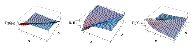
Figure 1: $R$ charges of $Q_{2}$, $F$ and $X_{1}$ without taking into account the operators hitting the unitarity bound.

Depending on the values of $x$ and $y$, some operators turn out to have $R$ charges below the free field value $2/3$. These operators should have been decoupled at lower values of $x$ and $y$. We propose a prescription, generalizing the one in [7], for decoupling these operators. Consider straight lines on the $xy$ plane starting from the point $(x,y)=(1,1)$ at various angles. Moving to the right and up along such a line from the point $(1,1)$, $\widetilde{Q}_{1}Q_{1}$ hits the unitarity bound first. Beyond this point along the line, we need to modify the trial $a$-function by subtracting the contribution of the decoupled operator and adding the contribution from a free field. As we proceed further on the line, more and more operators hit the unitarity bound and get decoupled, and each time this happens, we modify the trial $a$-function (see eq.(2.13)).

We can qualitatively see which operators hit the unitarity bound and get decoupled from the results in figure 1, by ignoring the modifications to the trial $a$-function. Our theory has several types of mesonic operators defined by $P_{l,1}=\widetilde{Q}_{1}X_{1}^{l-1}Q_{1}$, $M_{l,1}=\widetilde{Q}_{2}X_{2}^{l-1}{Q}_{2}$, $P_{l,2}=\widetilde{Q}_{1}X_{1}^{l-1}F{Q}_{2}$, $M_{l,2}=\widetilde{Q}_{2}X_{2}^{l-1}\widetilde{F}{Q}_{1}$, $P_{l,3}=\widetilde{Q}_{1}X_{1}^{l-1}F\widetilde{F}{Q}_{1}$, and $M_{l,3}=\widetilde{Q}_{2}\widetilde{F}FX_{2}^{l-1}{Q}_{2}$. Using the results above we see that the $R$ charges of the bifundamentals are greater than ${2\over 3}$ everywhere. The $R$ charges of the other chiral fields are positive, except that the $R$ charges of $Q_{1}$ and $Q_{2}$ become only slightly negative at large values of $x$ and $y$. Thus the mesonic operators that contain bifundamentals do not cross the unitarity bound, and only $P_{l,1}$ and $M_{l,1}$ can reach the bound. The region where the operators hit the bound is qualitatively depicted in figure 2.

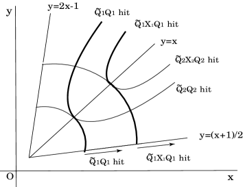
Figure 2: Qualitative picture of operators hitting the unitarity bound. Only $P_{l,1}=\widetilde{Q}_{1}X^{l-1}_{1}Q_{1}$ and $M_{l,1}=\widetilde{Q}_{2}X^{l-1}_{2}Q_{1}$ can saturate the bound.

We now follow the precise procedure described above and compute the $R$ charges exactly, including the back-reaction of the decoupled operators. We subtract from the trial $a$-function the contributions of the first $m$ $P_{l,1}$ and $n$ $M_{l,1}$ that hit the bound, and then add the corresponding contributions from as many free fields with the relation:

$$a^{(m,n)}\equiv a^{(0)}+{1\over 9}\sum_{l=1}^{m}[2-3R(P_{l,1})]^{2}[5-3R(P_{l,1})]+{1\over 9}\sum_{l=1}^{n}[2-3R(M_{l,1})]^{2}[5-3R(M_{l,1})],$$ (2.13)

where the $R$ charge of each operator can be expressed in terms of $R(Q_{1})$,

$$R(P_{l,1})=2R(Q_{1})+(l-1){2-2R(Q_{1})\over 2x-y},$$

$$R(M_{l,1})=2\left({x-2y\over y-2x}(R(Q_{1})-1)+1\right)+(l-1){2-2R(Q_{1})\over 2x-y}.$$ (2.14)

We also used the fact that

$$-[3(R-1)^{3}-(R-1)]+[3(\frac{2}{3}-1)^{3}-(\frac{2}{3}-1)]=\frac{1}{9}(2-3R)^{2}(5-3R)$$

in writing eq.(2.13).

$a^{(0)}$ can be evaluated at large values of $x$ and $y$:

$$a^{(0)}\simeq\!\!\!\!\!\! {1\over(2x-y)^{3}}\left[2(z-1)\left(8\left(3z^{2}-6z-2\right)x^{4}+\left(-39yz^{2}+78yz+5y\right)x^{3}\right.\right.$$ (2.15)

$$\left.\left.+18y\left(2yz^{2}-4yz+z-y\right)x^{2}+y^{2}\left(-39yz^{2}+78yz+2y\right)x\right.\right.$$

$$\left.\left.+2y^{3}\left(12yz^{2}-24yz+7y\right)\right)\right],$$

where $z\equiv R(Q_{1})$.

As we see from figure 2, a large number of $P_{l,1}$ hit the unitarity bound at large values of $x$ and $y$. In this limit, as in [7], we can approximate the first sum in eq.(2.13) by an integral:

$${1\over 9}\sum_{l=1}^{m}[2-3R(P_{l,1})]^{2}[5-3R(P_{l,1})]\simeq{1\over 27\beta}\int_{0}^{2-3\alpha}u^{2}(3+u)du={2\over 9}(2x-y)(1-3R(Q_{1}))^{3},$$ (2.16)

where $u\equiv 2-3R(P_{l,1})$, $\alpha\equiv 2R(Q_{1})$ and $\beta\equiv{2-2R(Q_{1})\over 2x-y}$. The situation is a little different for $M_{l,1}$. As seen from figure 2, not for all ratios of $x$ and $y$ do the operators $M_{l,1}$ hit the unitarity bound, making it difficult to calculate the second sum in eq.(2.13) in general. For this reason we will consider two limiting cases where the number of $M_{l,1}$ hitting the unitarity bound is either zero or very large.

The asymptotic forms of the $R$ charges and the central charge in the region near the line $y=(x+1)/2$, where only $P_{l,1}$ hit the unitarity bound, can be explicitly computed. The expressions right on the line $y={x+1\over 2}$ are simple to write and are given as as $R(Q_{1})\simeq-0.057$, $R(X_{1})\simeq 1.409x^{-1}$, and $a^{y=(x+1)/2}\simeq 10.36x$. Using these asymptotic values we see that $\mbox{Tr}X^{k}$ becomes relevant in the region $x>x_{k}=0.704k$. This provides one end of the conformal window on $y=(x+1)/2$. (The other is to be found from the analysis of the magnetic dual.)

Finally we will show that baryonic operators do not violate the unitarity bound on the line $y={x+1\over 2}$. To construct a baryonic operator we need enough number different quark superfields including dressed quark $(Q_{(I_{1}\cdots I_{n})})_{i}\equiv(X_{I_{1}}\cdots X_{I_{n}}Q)_{i}$. At a point $x=[x]$ we need $N=[x]N_{f}$ number of quarks to contract with indices of epsilon tensor. Therefore at least $([x]-1)N_{f}$ number of $X_{i}$ are included in baryonic operators. It is enough to consider the operator $B_{\rm small}\equiv\prod_{i=0}^{[x]-1}(X_{1}^{i}Q_{1})^{N_{f}}$ because this gives the smallest $R$ charge possessed by the baryonic operators. Since the order of the $R(B_{\rm small})$ is ${\cal O}(N)$, either $R(Q_{1})$ or $R(X_{1})$ have to be zero or negative to hit the bound. This can happen in the large $x$ region. Representing the $R(X_{1})$ in terms of $R(Q_{1})$ we have $R(B_{\rm small})\simeq N(R(Q_{1})+[x](1-R(Q_{1})))$. If we have a unitarity violation the condition, $R(Q_{1})+[x](1-R(Q_{1}))\simeq 0$ have to be satisfied. Since $R(Q_{1})$ varies within $-0.057\leq R(Q_{1})\leq 1$, however, it never hold. Therefore we conclude that there is no baryonic operator that hits the unitarity bound.

Next let us study the asymptotic behavior of the $R$ charges on the line $y=x$. If we restrict ourselves to the line $y={x}$ and large values of $x$, a large number of $M_{l,1}$ hit the bound. We obtain by the same approximation

$${1\over 9}\sum_{l=1}^{m}[2-3R(M_{l,1})]^{2}[5-3R(M_{l,1})]\Big{|}_{y=x}\simeq{2\over 9}x(1-3R(Q_{1}))^{3}.$$ (2.17)

Taking into account eqs. (2.13)-(2.17), we obtain the asymptotic values of the $R$ charges $R(Q_{1})\simeq-{1\over 8}$, $R(X_{1})={9\over 4x}$, and the central charge $a^{y=x}\simeq 26.81x$. One might worry again that baryonic operators may hit the unitarity bound. Proceeding in the same way as in the previous case, however, one can see that there is no baryonic operator hitting the bound. We conclude that the operator $\mbox{Tr}X_{1}^{k+1}$ becomes relevant in the region $x>x_{k}\equiv{9k\over 8}$.

Now that we have obtained the asymptotic behavior of the central charge $a$, we would like to test the $a$-theorem conjecture under the RG flow from $\widehat{D}$. In so doing we have to be careful about the arguments of functions. In [8], the central charge $a$ of the $\widehat{D}$ theory was expressed in terms of the variable $\widehat{x}\equiv{N\over N_{f}}$ while we are using $x={N_{1}\over N_{f}}$ and $y={N_{2}\over N_{f}}$ that satisfy the relation $\widehat{x}=x+y$. Thus comparing these results we have to use the variable $\widehat{x}$. Taking this point into account, we obtain

$$a^{y=(x+1)/2}(x)\Big{|}_{x={2\over 3}(\widehat{x}-{1\over 2})}\simeq 6.906\widehat{x},\qquad a^{y=x}(x)\Big{|}_{x=\widehat{x}/2}\simeq 13.40\widehat{x}.$$ (2.18)

The central charge of the $\widehat{D}$ theory was given in [8] as $a_{\widehat{D}}(\widehat{x})\simeq 13.40\widehat{x}$. By comparing these central charges we see that the $a$-theorem is satisfied under the RG flow:

$$a_{\widehat{D}}=a^{y=x}>a^{y=(x+1)/2}.$$ (2.19)

We see that the central charge on the line $y=x$ is equal to that of $\widehat{D}$ when $x$ is large. This is explained as follows. Let us assume that $N_{1}=N_{2}$, without assuming that $x=y$ is large. By comparing the superpotential eq.(2.9) with $\mbox{Tr}XY^{2}$ of $\widehat{D}$, we see that $X_{1}$ and $X_{2}$ play the role of $X$ in $\widehat{D}$, while $F$ and $\widetilde{F}$ play the role of $Y$, as far as the calculation of the trial $a$-function is concerned. Therefore central charge $a_{Higgsing}$ of the theory after Higgsing can be written as $a_{Higgsing}(N_{1},N_{2}=N_{1})=2a_{\widehat{D}}(N=N_{1})$ even before $a$-maximization. This relation translates to the relation $a_{Higgsing}(x,y=x)=2a_{\widehat{D}}(\widehat{x}=x)$, which holds even for finite values of $x$. Since in [8] the central charge $a_{\widehat{D}}$ of the $\widehat{D}$ theory was computed for finite values $x$, we can translate the result there to the central charge $a_{Higgsing}(x,y=x)$ of the theory after Higgsing with $x=y$. In the above we saw that $a_{Higgsing}(x,y=x)$ is linear in $x$ when $x$ is large. In this limit, we then have $a_{Higgsing}(x,y=x)\simeq 2^{-1}a_{Higgsing}(2x,y=2x)=a_{\widehat{D}}(\widehat{x}=2x)$ as we saw above.

As for the line $y={x+1\over 2}$ we have to calculate the central charge in detail, by following the procedure proposed early in this subsection. On this line only $P_{l,1}$ can hit the unitarity bound. For $x\gtrsim 1$, we take $a^{(0)}$ and maximize it. The obtained $R$ charges are correct up to $x\simeq 2.54$, where $P_{l=1,1}$ hits the unitarity bound. Above this value of $x$ we switch to $a^{(1,0)}$ and maximize it. Repeating the process in this way we see, for example, that the operators $P_{l,1}$ from $l=2$ to $6$ hit the bound at $x\simeq\ 4.29,\ 6.08,\ 7.88,\ 9.68$ and $13.38$. Patching the results together, we obtain the $R$ charges and the central charge up to ${N/N_{f}}=13.38$. The central charge of the $\widehat{D}$ theory, as well as those of the theories after Higgsing with $y=x$ and $y=(x+1)/2$ are depicted in figure 3. Clearly the results indicate the validity of the $a$-theorem conjecture in these Higgsing RG flows.

Figure 3: The figure on the left displays the $R$ charges $R(Q_{1})$ (top), $R(Q_{2})$ (middle), and $R(X_{1})$ (bottom) on the line $y={x+1\over 2}$. The figure on the right depicts the central charge of the $\widehat{D}$ theory (top) as well as those of the theories after Higgsing on the lines $y=x$ (middle) and $y={x+1\over 2}$ (bottom).

For later reference we calculate the value of $x$ at which $\mbox{Tr}X^{4}_{1}$ and $\mbox{Tr}X^{4}_{2}$ become relevant on the line $y={x+1\over 2}$. It turns out to be $x=1.879$, where no operator has decoupled by hitting the unitarity bound.

2.2 Analysis of the magnetic dual description

The magnetic dual description of the present model was proposed by Brodie in [18]. The dual gauge group is $U(3kN_{f}-N_{1})\times U(3kN_{f}-N_{2})$. The matter contents include $\overline{X}_{1},\overline{X}_{2},\overline{F}$, and $\widetilde{\overline{F}}$ that correspond to $X_{1},X_{2},F$, and $\widetilde{F}$ in the electric description, respectively. In addition, there are dual quarks $q_{1}$ and $q_{2}$, and the gauge singlets $P_{l,m}$ and $M_{l,m}$ ($m=1,2,3$) to be identified with the mesonic operators which have appeared in the electric description. The superpotential is [18]

$$W= \!\!\!\!\!\!\mbox{Tr}\overline{X}_{1}^{k+1}+\mbox{Tr}\overline{X}_{2}^{k+1}+\mbox{Tr}\overline{X}_{1}\widetilde{\overline{F}}{\overline{F}}+\mbox{Tr}\overline{X}_{2}\widetilde{\overline{F}}\overline{F}+\sum_{l=1}^{k}\left[M_{l,1}\widetilde{q}_{2}\overline{X}_{2}^{k-l}\overline{F}\widetilde{\overline{F}}q_{2}+P_{l,1}\widetilde{q}_{1}\overline{X}_{1}^{k-l}\widetilde{\overline{F}}\overline{F}q_{1}\right.$$ (2.20)

$$\left.+P_{l,2}\widetilde{q}_{2}\overline{X}_{2}^{k-l}\overline{F}q_{1}+M_{l,2}\widetilde{q}_{1}\overline{X}_{1}^{k-l}\widetilde{\overline{F}}q_{2}+M_{l,3}\widetilde{q}_{2}\overline{X}_{2}^{k-l}q_{2}+P_{l,3}\widetilde{q}_{1}\overline{X}_{1}^{k-l}q_{1}\right].$$

We define a new notation $\overline{N}_{1}\equiv 3kN_{f}-N_{1}$, $\overline{N}_{2}\equiv 3kN_{f}-N_{2}$, $\overline{x}\equiv{\overline{N}_{1}\over N_{f}}$ and $\overline{y}\equiv{\overline{N}_{2}\over N_{f}}$. Since we are interested in the parameter region where both factors of the gauge group in the magnetic theory are asymptotically free, we consider the following region;

$$2\overline{x}-1\geq\overline{y}\geq{(\overline{x}+1)\over 2}\iff{x+3k-1\over 2}\geq y\geq 2x-3k+1.$$ (2.21)

However since it is difficult to study the whole region, we will mostly focus on the lines $y=x$ and $y=2x-3k+1$. (See figure 4.)

Let us begin by studying the line $y=2x-3k+1$. We start from the point $\overline{x}=\overline{y}=1$ where both factors of the magnetic theory cease to be asymptotically free and become free in the IR. Thus all matter content have $R$ charge ${2\over 3}$ so only cubic terms in the superpotential can be marginal near the point,

$$W=\overline{X}_{1}\overline{F}\widetilde{\overline{F}}+\overline{X}_{2}\overline{F}\widetilde{\overline{F}}+M_{k,3}\widetilde{q}_{2}q_{2}+P_{k,3}\widetilde{q}_{1}q_{1}.$$ (2.22)

Taking into account the vanishing of the anomaly, we evaluate the $R$ charges away from the point, $(\overline{x},\overline{y})=(1,1)$. Trial $a$-function can be written as

$$a = 2\overline{x}^{2}+2\overline{y}^{2}+\overline{x}^{2}G[R(X_{1})]+2\overline{x}G[R(q_{1})]+2\overline{x}\overline{y}G[R(F)]+2\overline{y}G[R(q_{2})]$$ (2.23)

$$+\overline{y}^{2}G[R(X_{2})]+G[R(M_{k,3})]+G[R(P_{k,3})]+{2\over 9}(6k-2)$$

where we defined $G[x]\equiv 3(x-1)^{3}-(x-1)$. The last term comes from the free singlets. Among the all singlets only two are interacting, thus we have $6k-2$ free singlets. Away from the origin the $R$ charges of operators vary and some of the terms in the superpotential become relevant. As for the $k=3$ case, by using $a$-maximization, we can see that the operator $\mbox{Tr}\overline{X}_{1}^{4}$ and $\mbox{Tr}\overline{X}_{2}^{4}$ becomes marginal at $\overline{x}=1.422$. On the other hand, looking at $R$ charges of the fields we see that $M_{k-1,3}\widetilde{q}_{2}\overline{X}_{2}q_{2}$ becomes marginal next at $\overline{x}=1.452$. Thus before this term becomes relevant $\mbox{Tr}\overline{X}_{1}^{4}$ and $\mbox{Tr}\overline{X}_{2}^{4}$ become relevant and thus the conformal window starts from $\overline{x}=1.422$ . Combining the results we can roughly draw the conformal window as in figure 4.

Next let us study the asymptotic behaviors on this line, $y=2x-3k+1$. At $(\overline{x},\overline{y})=(1,1)$ the $R$ charges of all fields are ${2\over 3}$. First since only cubic superpotential can be marginal, we maximize $a$-function while imposing the marginality of the superpotential (2.22) and the ABJ anomaly cancellation. To see the behavior we calculated several values of $k$ and found that $R(q_{1})$ and $R(F)$ are monotonically increasing functions and take values greater than ${2\over 3}$. On the other hand $R(q_{2})$ and $R(\overline{X}_{1})=R(\overline{X}_{2})$ are monotonically decreasing functions. Also all the $R$ charges are positive. Thus among the superpotential terms (2.20) including more than two of $q_{1}$ and $F$ can not be relevant. Only $M_{l,3}\widetilde{q}_{2}\overline{X}_{2}^{k-1}q_{2}$ become relevant and the point where it becomes marginal is given by the solution to the equation,

$$2R(q_{2})+(p-1)R(\overline{X}_{2})={4\over 3}.$$ (2.24)

where $p$ is the number of superpotential terms which are marginal. In other words we assume that first $k-p$ singlets $M_{1,3},\cdots M_{k-p,3}$ are free.

First let us calculate asymptotic behavior of the contribution coming from interacting $M_{l,3}$. Using the marginality of superpotential we can rewrite the summation of $l=k-p+1,\cdots k$ by $j=1,\cdots p$ as follows:

$$\sum_{l=k-p+1}^{k}G[R(M_{l,3})] = \sum_{j=1}^{p}G[2-R(\widetilde{q}_{2}\overline{X}_{2}^{k-l}q_{2})]$$ (2.25)

$$= {1\over 9}\sum_{l=1}^{p}\left(2-3R(N_{l,3})\right)^{2}\left(5-3R(N_{l,3})\right)-{2\over 9}p$$

where we defined $N_{j,3}\equiv\widetilde{q}_{2}\overline{X}_{2}^{p-j}q_{2}$ and the relation noted just above $(2.13)$. From the vanishing of the anomaly and the marginality of the superpotential $\overline{X}_{2}\overline{F}\widetilde{\overline{F}}$, the $R$ charge of $\overline{X}_{2}$ is written in terms of $R(q_{2})$ as $R(\overline{X}_{2})={2-2R(q_{2})\over 3\overline{x}-2}$. At large $\overline{x}$ variable $u$ defined by

$$u\equiv 2-3R(N_{j,3})=2-3\left(2R(q_{2})+(p-j){2-2R(q_{2})\over 3\overline{x}-2}\right)$$ (2.26)

becomes continuous. Therefore we can approximate the contributions of $M_{l,3}$ by an integral. Using (2.24) we see that $u$ vary within $[-2,2-6R(q_{2})]$. Thus contribution of the interacting $M_{l,3}$ (2.25) can be written by an integral as follows:

$$\sum_{l=k-p+1}^{k}G[R(M_{l,3})] \simeq {\overline{x}\over 18(1-R(q_{2}))}\int_{-2}^{2-6R(q_{2})}du\,u^{2}(3+u)-{2\over 9}p$$ (2.27)

$$= {2\overline{x}\over 3}(1-3R(q_{2}))^{3}+{2\overline{x}\over 9(1-R(q_{2}))}-{2\over 9}p.$$

Note that using (2.25) we can represent the $p$ in terms of $R(q_{2})$ as $p\simeq{2-3R(q_{2})\over 1-R(q_{2})}\overline{x}$. Another contributions to the trial $a$-function can be written as

$$a = 2\overline{x}^{2}+2\overline{y}^{2}+\overline{x}^{2}G[R(X_{1})]+2\overline{x}G[R(q_{1})]+2\overline{x}\overline{y}G[R(F)]+2\overline{y}G[R(q_{2})]$$ (2.28)

$$+\overline{y}^{2}G[R(X_{2})]+G[R(P_{k,3})]+{2\over 9}(6k-1-p)$$

$$\simeq 12R(q_{2})^{3}-36R(q_{2})^{2}+4R(q_{2})+20+{2\over 9}(6k-p)$$

Adding (2.27) and (2.28) we obtain the trial $a$-function at large values of $\overline{x}$. By maximizing it we obtain $R(q_{2})\simeq-0.0391$. Using this result we see that $\mbox{Tr}X_{1}^{k}$ becomes relevant at $\overline{x}\simeq 0.346k$ equivalently $x\simeq 2.65k$. Plugging these $R$ charges back into the central charge gives $a^{mag}\simeq 20.02\overline{x}+{4k\over 3}$.

Let us now turn to the magnetic description on the line $y=x$. By the same argument as in the previous subsection, the central charge on this line is related to that of $D_{k+2}$ by $a^{mag}_{Higgsing}(\overline{N}_{1},\overline{N}_{2}=\overline{N}_{1})=2a_{{D}_{k+2}}^{mag}(\overline{N}=\overline{N}_{1})$ if we identify $\overline{N}=3kN_{f}-N$ in [8] with $\overline{N}_{1}$ in our model. To rewrite the central charge $a^{mag}_{Higgsing}$ in terms of $\widehat{\overline{x}}\equiv{\overline{N}\over N_{f}}$ we use the relation $\widehat{\overline{x}}=2\overline{x}-3k$. Therefore by using the results for the dual of $D_{k+2}$, we obtain the central charge of our magnetic dual as $a^{mag}_{Higgsing}(\overline{x}=(\widehat{\overline{x}}+3k)/2,\overline{y}=\overline{x})=2a_{D_{k+2}}^{mag}(\widehat{\overline{x}})$. To begin with let us consider the large $\overline{x}$ behavior of the central charge and look for a point where the operators $\mbox{Tr}\overline{X}_{1}^{k+1}$ and $\mbox{Tr}\overline{X}_{2}^{k+1}$ become marginal. Using the result $a^{mag}_{D_{k+2}}(\widehat{\overline{x}})\simeq 13.1186\widehat{\overline{x}}+{6k\over 9}$ given in [8], we obtain $a_{Higgsing}^{mag}(\overline{x}=(\widehat{\overline{x}}+3k)/2,\overline{y}=\overline{x})\simeq 13.1186\widehat{\overline{x}}+40.68k$. The point where $\mbox{Tr}\overline{X}_{1}^{k+1}$ becomes relevant is ${\overline{N}_{1}\over N_{f}}\simeq 1.1038k$. To compute the conformal window of the $D_{5}$ theory, let us see where $\mbox{Tr}X^{4}_{1}$ becomes marginal. From [8] $\overline{x}_{5}^{min}\simeq 2.09$ thus the conformal window starts at $3k-1-\overline{x}_{5}^{min}\simeq 7.14$.

Combining the analysis of the electric and magnetic descriptions, we obtain the conformal window in the large $k$ case.

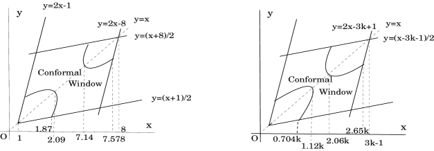
Figure 4: Conformal windows of the theories with $k=3$ and $k\gg 1$. In each graph, we computed the numerical values of $x$ at the corners of the conformal window and interpolated between the corners by hand.

3 Higgsing of the E-type Fixed Points

In this section we study Higgsing of the $E$-type theories. In all the $E$-type models the $F$-term condition demands that the vev of $Y$ be zero.

3.1 Higgsing $\widehat{E}$

We consider Higgsing $U(N)\rightarrow U(N_{1})\times U(N_{2})$ of the $\widehat{E}$ theory by the vev eq.(2.8) of the adjoint $X$, which is allowed by the $F$- and $D$-term conditions. For the notation for the fields that arise, see section 2. Bifundamentals coming from the fluctuations of $X$ become massive while $X_{1},X_{2},Y_{1},Y_{2},F,\widetilde{F}$, $Q_{1},Q_{2},\widetilde{Q}_{1}$, and $\widetilde{Q}_{2}$ remain massless. In this case, however, at least one of the gauge group factors is asymptotically non-free and becomes non-interacting in the IR. When just one factor is asymptotically free, the analysis of the model proceeds in exactly the same way as in the $\widehat{A}$ case for the reasons we now explain. After Higgsing we have the superpotential

$$W=\mbox{Tr}Y_{1}^{3}+\mbox{Tr}Y_{2}^{3}+\mbox{Tr}Y_{1}F\widetilde{F}+\mbox{Tr}Y_{2}\widetilde{F}F.$$ (3.29)

Assuming that $N_{1}-N_{2}>N_{f}$, only $SU(N_{1})$ is asymptotically free and has $N_{f}+N_{2}$ quarks, two kinds of singlets $Y_{2},X_{2}$ and two adjoints $X_{1}$ and $Y_{1}$. Since the superpotential has $R$ charge two all the fields that appear in the superpotential have $R={2\over 3}$. Thus the gauge singlets can be regarded as free fields as far as the computation of the trial $a$-function is concerned. Also we have to consider the anomaly cancellation condition

$$N_{1}R(X_{1})+N_{f}R(Q_{1})-N_{f}-{N_{1}+N_{2}\over 3}=0.$$ (3.30)

The trial $a$-function can be written as

$$a=a_{\rm int}(X_{1},Q_{1})+a(X_{2})+a(Y_{1})+a(Y_{2})+a(Q_{1}^{\prime}).$$ (3.31)

The last four contributions are computed by regarding the singlets as free fields. Thus the only difference from $\widehat{A}$ is the constant term ${-N/3}$ in the anomaly cancellation condition eq.(3.30). Maximizing the trial $a$-function with respect to $R(Q_{1})$ yields

$$R(Q_{1})=\frac{6x^{2}+2x-y-\sqrt{10x^{4}-8yx^{3}+2y^{2}x^{2}-x^{2}}-3}{3\left(2x^{2}-1\right)}.$$ (3.32)

Because $R(Q_{1})$ and $R(X_{1})$ are monotonically decreasing function of $x,y$ and satisfy $R(Q_{1})>{2\over 3}$ and $R(X_{1})>{2\over 3}$ for all region $y<x-1$. Therer is thus no reason to doubt the validity of the above experssions. With the central charge of $\widehat{E}$ shown in [8] we verified $a-$theorem conjecture.

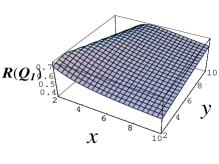
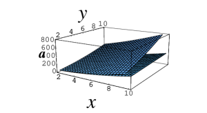
Figure 5: The first figure displays $R$ charge $R(Q_{1})$ as a function of $x$ and $y$. The second figure shows the central charge of $\widehat{E}$ theory and Higgssed theory.

3.2 Higgsing $E_{7}$

Let us turn to Higgsing of the $E_{k},~{}k=6,7,8$ theories. In the $E_{6}$ and $E_{8}$ theories, their superpotentials do not admit non-zero vevs of $X$ or $Y$, and there is no Higgsing RG flow allowed. he superpotential $\mbox{Tr}(XY^{2}+Y^{3})$ of $E_{7}$ does allow us to give a vev to $X$ and admits several breaking patterns: If we take eq.(2.8) with generic values of $a$ and $b$, the bifundamentals coming from the fluctuations of $X$ and $Y$, as well as $Y_{1}$ and $Y_{2}$, are massive and get integrated out. Thus the theory flows to a $SU(N_{1})\times SU(N_{2})$ theory with massless fields $X_{1},X_{2}$, $Q_{1}$, and $Q_{2}$ and a vanishing superpotential. This is a product of two copies of $\widehat{A}$. Using the data for $E_{7}$ [8] and $\widehat{A}$ [7], we verified that the $a$-theorem is satisfied under the RG flow. If we take one of vev’s in $(\ref{VEVX})$ to be zero, say $a=0$, $Y_{1}$ remains massless and there exists a superpotential $\mbox{Tr}Y_{1}^{3}$. However this model is still not interesting because it is just a product of $\widehat{E}$ and $\widehat{A}$ without any interactions between them. Again by using the results in [8] we explicitly checked the $a$-theorem prediction.

The most interesting possibility is the $a=-b\neq 0$ case. In this case the mass terms for bifundamentals $F$ and $\widetilde{F}$ coming from $Y$ cancel out. Therefore the bifundamentals $F$ and $\widetilde{F}$ as well as the adjoint fields $X_{1}$ and $X_{2}$ and the fundamentals $Q_{1},Q_{2}$ remain massless. Also there are superpotential terms constructed from the bifundamentals:

$$W=\mbox{Tr}(F\widetilde{F})^{2}+{\rm higher\ order\ terms}.$$ (3.33)

When we integrated out the massive fields $Y_{1}$ and $Y_{2}$ we used the equation of motion. We drop the higher-order terms, which are irrelevant when the lowest order term is marginal. In the rest of the subsection, we focus on this model.

The requirement that the superpotential has $R$ charge two yields $R(\widetilde{F})=R(F)={1\over 2}$. The anomaly cancellation conditions are

$$xR(X_{1})+R(Q_{1})-{y\over 2}=1,\qquad yR(X_{2})+R(Q_{2})-{x\over 2}=1.$$ (3.34)

we are left with two undetermined $R$ charges. To fix them we use $a$-maximization. The trial $a$-function is

$$a^{(0)}=a[R(X_{1}),x,y]+a[R(X_{2}),y,x]+{1\over 8}xy,$$ (3.35)

where the last term comes from the contributions of bifundamentals and we defined the function $a[R,x,y]$ by

$$a[R,x,y]\equiv 2x^{2}+x^{2}\left(3(R-1\right)^{3}-(R-1))+2x\left(3(xR-{y\over 2})^{3}-(xR-{y\over 2})\right).$$ (3.36)

Maximizing the trial $a$-function with respect to $R(X_{1})$ and $R(X_{2})$, we obtain the $R$ charges of the fields. The expression of $R(Q_{1})$ is relatively simple:

$$R(Q_{1})=\frac{12x^{2}+6x-3y-6-x\sqrt{2\left(40x^{2}-36yx+9y^{2}-2\right)}}{12x^{2}-6}.$$ (3.37)

$R(Q_{2})$ can be obtained by replacing $x$ with $y$ in $R(Q_{1})$. Using these results it is easy to see that in the region where both gauge groups are asymptotically free, there are no gauge invariant operators that hit the unitarity bound. Therefore our results do not receive corrections due to operators hitting the unitarity bound.

The central charge $a(x,y)$ is shown in fig 6. With this function we can check the $a$-theorem conjecture under the Higgsing RG flow. For simplicity we check the validity of the conjecture on the lines $y=2x-1$ and $y={x+1\over 2}$, which are the bounds of asymptotic freedom. In so doing, as in the previous section, we need to be careful about the arguments of the $a$-function. For example, when we draw the figure for the central charge on $y=2x-1$, we use $a(x,2x-1)|_{x={\widehat{x}+1\over 3}}$, where $\widehat{x}\equiv N/N_{f}$, to compare with the central charge of the $E_{7}$ theory. As we see from figure 6 the $a$-theorem is satisfied under this Higgsing RG flow.

The region where the Higgsed model is interacting and conformal may be narrower than that determined by asymptotic freedom of the gauge groups above, although we find nothing that suggests this. If there exists a magnetic description of the $E_{7}$ theory, it should be possible to find this region (conformal window) in a way similar to what we did in the $D$-type case.

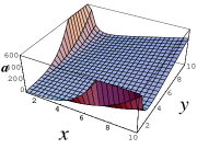
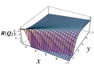
Figure 6: The first two figures display the central charge $a$ and the $R$ charge $R(Q_{2})$ as functions of $x$ and $y$. Near the edges of the figures the functions vary abruptly. These points are all outside of the region where both gauge groups are asymptotically free and are of no significance. The third figure shows the central charges of the $E_{7}$ theory, the Higgsed theories on the $y=2x-1$ slice and the $y={x+1\over 2}$ slice from the top to the bottom. The $a$-theorem is satisfied.

4 Superpotential Deformations of $\widehat{O}$

We start considering mesonic superpotential deformations. This section and the following ones can be read independently of the previous ones.

4.1 Deformations of $\widehat{O}$ by mesonic superpotential terms

The authors of [8] studied the RG fixed point, which was called $\widehat{O}$, of the two-adjoint SQCD with $W=0$ by using $a$-maximization and calculated the superconformal $U(1)$ $R$ charges and central charge $a$. $R(X)=R(Y)$ and $R(Q)$ are monotonically decreasing functions of $x=N/N_{f}$ and take values $0.5\lesssim R(X)<2/3$ and $0.575\lesssim R(Q)<2/3$. Among the operators that preserve the diagonal $SU(N_{f})$, there are two relevant mesonic superpotential deformations $\widetilde{Q}_{i}XQ^{i}\ ({\rm or~{}equivalently}\ \widetilde{Q}_{i}YQ^{i})$ and $\widetilde{Q}_{i}Q^{i}$ for all $x>1$. We see that there is no relevant deformation that includes more than two quark superfields. First let us consider the deformation by $W=\widetilde{Q}_{i}XQ^{i}$, which we expect leads to a new fixed point that we refer to as $\widehat{M}$. At the fixed point the $R$ charge of $W$ has to be two, and the $U(1)_{R}$-$SU(N_{i})$-$SU(N_{i})$ ABJ anomaly has to vanish. Thus we have the following two constraints for three independent charges, leaving one flavor $U(1)$ symmetry at the new fixed point. .

$$2R(Q_{i})+R(X)=2,\qquad\ \ \ R(Q_{i})+xR(X)+xR(Y)-x-1=0.$$ (4.1)

To determine the superconformal $R$ symmetry we use $a$-maximization. Maximizing the trial $a$-function gives

$$R(X)=\frac{24x^{3}-2x{\sqrt{-1-12x+98x^{2}-180x^{3}+144x^{4}}}}{3-18x+30x^{2}}.$$ (4.2)

Using this result one can check if there is a gauge invariant operator that hits the unitarity bound. As discussed in [7], ${\rm Tr}X^{i}$ or ${\rm Tr}Y^{k}$ do not contribute to the central charge in the large $N$ limit (1.2), because the contributions from these operators are ${\cal O}(N_{f}^{0})$ although the central charge $a$ is ${\cal O}(N_{f}^{2})$. Generalized mesons and generalized baryons

$${\cal M}_{I_{1}\cdots I_{n}}=\widetilde{Q}_{i}X_{I_{1}}\cdots X_{I_{n}}Q_{i},\qquad B=Q_{(I_{1}\cdots I_{n_{1}})}^{n_{(I_{1}\cdots I_{n_{1}})}}Q_{(J_{1}\cdots J_{n_{1}})}^{n_{(J_{1}\cdots J_{n_{1}})}}\cdots Q_{(K_{1}\cdots K_{n_{1}})}^{n_{(K_{1}\cdots K_{n_{1}})}}$$ (4.3)

do contribute to the central charge $a$. Here $\left(Q_{(I_{1}\cdots I_{n})}\right)_{i}\equiv(X_{I_{1}}\cdots X_{I_{n}}Q)_{i}$ and $N=n_{(I_{1}\cdots I_{n_{1}})}+\cdots+n_{(K_{1}\cdots K_{n_{1}})}$. The $R$ charges and the central charge $a$ are shown in figure 7. From figure 7 we see that $R(Q_{i})>0.65$ and conclude that in our new fixed point $\widehat{M}$ there is no meson or baryon that hits the unitarity bound. Thus for all $x>1$, our results do not receive corrections due the decoupling of operators hitting the unitarity bound. Also we see that the $a$-theorem conjecture holds under the RG flow. This is as anticipated because we expect that the Lagrange multiplier method of [10] should work in this case. Still, there is no general proof of the $a$-theorem for superpotential deformations, and our results are an addition to the already huge accumulation of evidence supporting the conjecture.

Let us consider generalized baryonic operators hitting the unitarity bound. Since a baryonic operator includes $N$ quark superfields $Q_{i}$, in the large $N$ limit the $R$ charge is of the order ${\mathcal{O}}(N_{f})$. Thus a generalized baryon can hit the unitarity bound only when $R(Q)$ is very small. Namely $R(Q)=0$ indicates baryonic operators hitting the unitarity bound.

Figure 7: The graph on the left displays the $R$ charges $R(Q)$ (top), $R(X)$ (middle), and $R(Y)$ (bottom). The graph on the right shows the central charges $a_{\widehat{O}}$ (top) and $a_{\widehat{M}}$ (bottom). Since the difference is very small the graph is magnified near $x\simeq 10$. There is no violation of the $a$-theorem conjecture anywhere inside or outside of the region shown.

What was found in [8] for their models was that the following consequences of the $a$-theorem are violated outside the conformal window: $a(N,N_{f})>a(N,N_{f}-1)$. The inequality comes from integrating out a quark. In the large $N$ limit (1.2) they can be stated as [8]

$${a(x)\over x^{2}} \qquad{\rm must\ be\ a\ monotonically\ decreasing\ function\ of\ }x.$$ (4.4)

Note our convention of $a$ (1.3). We verified that the conditions in eq.(4.4) are satisfied.

Next let us study the mass deformation $W=\widetilde{Q}_{i}Q^{i}$. Since quarks are decoupled, we have an asymptotically free gauge theory with two adjoints. We thus expect the theory to be at a nontrivial fixed point that we name ${M}^{\widehat{M}}_{(0,0)}$. The ABJ anomaly cancellation condition can be written as $R(X)+R(Y)=1$. After $a$-maximization we obtain $R(X)=R(Y)={1\over 2}$ and $a^{\widehat{M}}_{(0,0)}(x)={9\over 4}x^{2}$. One can see from figure 8 that the $a$-theorem conjecture holds for the flow $\widehat{O}\rightarrow M^{\widehat{M}}_{(0,0)}$. In this model we can construct exactly marginal operators $\mbox{Tr}X^{2}Y^{2}$ and $\mbox{Tr}XYXY$ [14]. Note that with $R$ charges obtained above we see that $\mbox{Tr}X^{4}$ is also a marginal operator. However since it breaks the global symmetry that mix the $X$ and $Y$, $\mbox{Tr}X^{4}$ can not be an exactly margianl operator.

Figure 8: Central charge $a$ at $M^{\widehat{M}}_{(0,0)}$ (bottom) and $\widehat{O}$ (top).

In the ${M}^{\widehat{M}}_{(0,0)}$ theory, since quarks have been integrated out there are no mesons or baryons. As we mentioned in the $\widehat{M}$ case, operators such as $\mbox{Tr}X^{l}$ do not contribute to $a$ in the large $N$ limit. We thus need not consider the effects of operators hitting the unitarity bound. We checked that the conditions in eq.(4.4) are satisfied for the ${M}^{\widehat{M}}_{(0,0)}$ theory, and we find nothing that suggests the existence of a stability bound.

There are several relevant deformations $\mbox{Tr}Y^{2},\ \mbox{Tr}XY^{2}$ for all $x>1$ at $M^{\widehat{M}}_{(0,0)}$. If we assume that these give rise to new fixed points, we are led to unnatural $R$ charge assignments: $R(Y)=1,\ R(X)=0,\ a(x)=0$. We thus rather conclude that these deformations do not lead to non-trivial fixed points. Below, we will meet this type of relevant deformations several times. In such a case we simply ignore them. Finally we comment on two-adjoint models realized by D-branes in some Calabi-Yau geometries [13]. These models have superpotentials, constructed from two adjoints, which can take the forms we study here. As seen above among the generic monomial superpotential of the theories only $\mbox{Tr}Y^{2}$ and $\mbox{Tr}XY^{2}$ can be relevant at UV theories. However ABJ anomaly cancellation condition and marginality of the superpotential give a vanishing central charge $a(x)=0$. Therefore we conclude that such models do not have interacting conformal fixed points.

4.2 Deformations of $\widehat{M}$ by $\mbox{Tr}X^{m}Y^{n}$

In this subsection we consider the deformations of $\widehat{M}$ by $\Delta W=\mbox{Tr}X^{m}Y^{n}$. Using the $R$ charges (4.1) and (4.2) at $\widehat{M}$, we obtain seven relevant operators, $\mbox{Tr}X^{m}Y^{n}$ with $1<m+n\leq 3$ for all range $x>1$. All these operators have no more than three adjoint fields so there is no multi-trace operator which give rise to a manifold of fixed points.

4.2.1 $\widehat{M}\rightarrow M^{\widehat{A}}_{(4,0)}$

We begin with the adjoint mass term $\mbox{Tr}X^{2}$. $X$ becomes massive and gets integrated out. The equation of motion for $X$ is $2X_{\alpha\beta}+(Q^{i}\widetilde{Q}_{i})_{\alpha\beta}=0$. Substituting the result into the original superpotential we obtain a one-adjoint SQCD with $W=-{1\over 2}\widetilde{Q}_{j}Q^{i}\widetilde{Q}_{i}Q^{j}$. We call this new fixed point $M^{\widehat{A}}_{(4,0)}$. Here we see that there exists an operator that consists of the same fields with different contractions of flavor indices $\widetilde{Q}_{i}Q^{i}\widetilde{Q}_{j}Q^{j}$. $\widetilde{Q}_{j}Q^{i}\widetilde{Q}_{i}Q^{j}$ combined with $\widetilde{Q}_{i}Q^{i}\widetilde{Q}_{j}Q^{j}$ produce a line of fixed points.

4.2.2 $\widehat{M}\rightarrow M^{\widehat{D}}_{(0,1)}$

We now turn to the $\mbox{Tr}X^{2}Y$ deformation. Since we have two superpotential terms, there are two possibilities: 1)We keep the $R$ charges of both terms to be two. 2) We only keep the $R$ charge of the deformation $\mbox{Tr}X^{2}Y$ to be two and the other term $\widetilde{Q}_{i}XQ^{i}$ becomes irrelevant under the RG flow. It is worth noting that decreasing of central charge $a$ under the second assumption is not obvious a priori thought it is clear for the first one from the $a$-maximization point of view. We computed the $R$ charge of $\widetilde{Q}_{i}XQ^{i}$ under the assumption 2) and found that it is smaller than two, leading to a contradiction. Thus the first scenario must happen, where we keep both terms. The flavor $U(1)$ symmetry is now broken, and $R$ charges can be determined without using $a$-maximization: $R(Q)={x+1\over 2x+1}$, $R(X)={2x\over 2x+1}$, and $R(Y)={2\over 2x+1}$. We name this new fixed point $M^{\widehat{D}}_{(0,1)}$. We see that $R(Q)>0.5$ and conclude that there is no unitarity bound violation by operators including quarks. The central charge is

$$a^{\widehat{D}}_{(0,1)}(x)=\frac{2x^{2}\left(2+2x+35x^{2}\right)}{{\left(1+2x\right)}^{3}}.$$ (4.5)

From figure 9 we verify that the $a$-theorem holds for the flow $\widehat{M}\rightarrow M^{\widehat{D}}_{(0,1)}$ . We also checked that the conditions in eq.(4.4) hold.

Figure 9: The graph on the left shows the $R$ charges $R(X)$ (top), $R(Q)$ (middle) and $R(Y)$ (bottom) at the $M^{\widehat{D}}_{(0,1)}$ fixed point. The graph on the right depicts the central charges at the fixed points $\widehat{M}$ (top) and $M^{\widehat{D}}_{(0,1)}$ (bottom).

4.2.3 $\widehat{M}\rightarrow M^{\widehat{E}}_{(1,0)}$ and $\widehat{M}\rightarrow M^{\widehat{E}}_{(0,1)}$

Next let us study $\mbox{Tr}Y^{3}$ and $\mbox{Tr}X^{3}$ deformations. Proceeding in the same way as in the previous cases we see that these deformations drive the theory from $\widehat{M}$ to new interacting CFT points that we name $M^{\widehat{E}}_{(1,0)}$ and $M^{\widehat{E}}_{(0,1)}$, respectively. The $R$ charges at $M^{\widehat{E}}_{(1,0)}$ are $R(Q)={5x-3\over 3(2x-1)}$, $R(X)={2x\over 3(2x-1)}$, and $R(Y)={2\over 3}$. At $M^{\widehat{E}}_{(0,1)}$, we have $R(Q)={2\over 3}$, $R(X)={2\over 3}$, and $R(Y)={x+1\over 3x}$. In both cases neither baryons nor mesons hit the unitarity bound. Thus we do not have to consider operators hitting the unitarity bound. The central charge $a$ can be written as follows and satisfy the $a$-theorem (figure 10) and eq.(4.4):

$$a^{\widehat{E}}_{(1,0)}(x)=\frac{2\,x^{2}\,\left(2+18\,x-79\,x^{2}+72\,x^{3}\right)}{9\,{\left(-1+2\,x\right)}^{3}},\quad a^{\widehat{E}}_{(0,1)}(x)=\frac{-6x+1+13x^{2}+18x^{3}}{9x}$$ (4.6)

Figure 10: The solid line on the left graph is $a^{\widehat{E}}_{(1,0)}$ and that on the right graph is $a^{\widehat{E}}_{(0,1)}$. The dashed line is $a_{\widehat{M}}$ in both graphs.

4.2.4 Other deformations

Finally let us study the remaining deformations, which do not drive to interacting CFT points. First we consider the deformation $\Delta W=\mbox{Tr}Y^{2}$ . Since this is a mass term, $Y$ gets decoupled under the flow. Thus the theory becomes a one-adjoint SQCD with the superpotential $\widetilde{Q}_{i}XQ^{i}$. We expect that this theory is not an interacting CFT because $R(X)=0$ and $a(x)=0$ as discussed the previous subsection. As for $\Delta W=\mbox{Tr}XY$, integrating out the $X$ and $Y$ leaves a vanishing superpotential. Therefore we obtain a pure SQCD, for which the region $x>1$ is out of the conformal window. Likewise using the ABJ anomaly cancellation condition and marginality of superpotential $\Delta W=\mbox{Tr}XY^{2}$ we conclude that it does not drive the theory to a new interacting CFT point.

Let us consider further meson deformations of $\widehat{M}$. The chiral ring relations $\widetilde{Q}_{i\alpha}Q^{i\beta}=0$ imply that all the meson operators are trivial at $\widehat{M}$. Thus most mesons can be excluded from relevant operators. The mass deformation $\widetilde{Q}_{i}Q^{i}$ is, however, relevant, corresponding to the constant shift of $X$. See footnote 5. The theory then flows to $M^{\widehat{M}}_{(0,0)}$.

In this section we have considered several flows from the $\widehat{O}$ and obtained new interacting fixed points. These flows and fixed points are summarized in figure 11. As we will see later all these new fixed points also arise by mesonic superpotential deformations of $\widehat{A}$, $\widehat{D}$, and $\widehat{E}$.

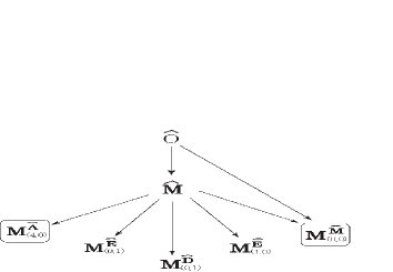
Figure 11: New interacting superconformal fixed points and flows. The squar means that there exists an exactly margianl operator in all region of the RG-fixed point.

5 Superpotential Deformations of $\widehat{E}$

5.1 Deformations of $\widehat{E}$ by mesonic superpotential terms

In this section we study mesonic superpotential deformations of the fixed point $\widehat{E}$, which is characterized by $W=\mbox{Tr}Y^{3}$. The authors of [8] discussed deformations of the form $\Delta W={\rm Tr}X^{m}Y^{n}$. We extend their study to deformations by mesonic terms. From the data for $\widehat{E}$ in table 1, taken from [8], and by taking the chiral ring relation $Y^{2}=0$ into account, we see that there are eight mesonic terms that become relevant for some values of $x$: $\Delta W=\widetilde{Q}_{i}XYQ^{i},\widetilde{Q}_{i}YXQ^{i},\widetilde{Q}_{i}YQ^{i},\widetilde{Q}_{j}Q^{i}\widetilde{Q}_{i}Q^{j}$, and $\widetilde{Q}_{i}X^{l}Q^{i}$ with $0\leq l\leq 3$ . The symbols for these deformations were defined in eq.(1.5). In the regions where these operators are relevant, see table 1. We have to pay attention to the order of $X$ and $Y$. $\widetilde{Q}_{i}XYQ^{i}$ and $\widetilde{Q}_{i}YXQ^{i}$ are distinct operators, and we expect that they give rise to a line of fixed points by the argument given in the introduction. Also $\widetilde{Q}_{j}Q^{j}\widetilde{Q}_{i}Q^{i}$ combines with the fourth operator to yields a line of fixed points. The anomaly cancelation and the marginality of $W={\rm Tr}Y^{3}+\Delta W$ is enough to determine the $R$ charges $R(Q_{i})$, $R(Y)$ and $R(X)$ without using $a$-maximization. From the $R$ charges, one can determine the range of $x$ where $\Delta W$ is relevant. We checked that there is no operator hitting the unitarity bound in this range for the flow from $\widehat{E}$ to each fixed point. These results are summarized in table 1. One can verify from the sample values of $a$ given in the table that all the flows satisfy the conjectural $a$-theorem. To be complete, we list the $a$-functions at the fixed points.

$$a_{(3,0)}^{\widehat{E}}={2x^{2}(8x^{3}-29x^{2}+18x+6)\over(2x-3)^{3}} a_{(2,0)}^{\widehat{E}}={x^{2}(18x^{3}-41x^{2}+18x+4)\over 9(x-1)^{3}},$$ ,

$$a_{(1,0)}^{\widehat{E}}={2x^{2}(72x^{3}-79x^{2}+18x+2)\over 9(2x-1)^{3}} a_{(0,1)}^{\widehat{E}}={18x^{3}+13x^{2}-6x+1\over 9x},$$ ,

$$a_{(1,1)}^{\widehat{E}}={2x^{2}(8x^{3}-5x^{2}-10x+6)\over(2x-1)^{3}} a_{(0,0)}^{\widehat{E}}=2x^{2},$$ , (5.1)

$$a^{\widehat{E}}_{(4,0,0)}(x)=-\frac{3}{2}+\frac{3}{8\,x}+\frac{7\,x}{4}+2\,x^{2}.$$

Note that at $M^{\widehat{E}}_{(0,0)}$ $R(X)$ is independent of $x$. One can check that the beta function for the gauge coupling and the beta functions for $\mbox{Tr}X^{4}Y$ and $\mbox{Tr}X^{6}$ are linearly dependent, giving rise to a line of fixed points.

	$W$	$R(X)$	$R(Q)\equiv y$	relevant	$a(50)$	$a(30)$
$\widehat{E}$	${\rm Tr}Y^{3}$	${1+x-y\over x}-{2\over 3}$	${1+{x(2-\sqrt{10x^{2}-1})\over 3(2x^{2}-1)}}$	$x>1$	$5086.20$	$1851.08$
${M}_{(3,0)}^{\widehat{E}}$	${\rm Tr}Y^{3}+\widetilde{Q}_{i}X^{3}Q^{i}$	${2x\over 3(-3+2x)}$	${x-3\over 2x-3}$	$x\geq 40.8$	$5086.19$	$1851.06$
${M}_{(2,0)}^{\widehat{E}}$	${\rm Tr}Y^{3}+\widetilde{Q}_{i}X^{2}Q^{i}$	${x\over 3(-1+x)}$	${2x-3\over 3(x-1)}$	$x\geq 3.7$	$5072.54$	$1843.63$
${M}_{(1,0)}^{\widehat{E}}$	${\rm Tr}Y^{3}+\widetilde{Q}_{i}XQ^{i}$	${2x\over 3(-1+2x)}$	${5x-3\over 3(2x-1)}$	$x>1$	$5040.49$	$1824.38$
${M}_{(0,1)}^{\widehat{E}}$	${\rm Tr}Y^{3}+\widetilde{Q}_{i}YQ^{i}$	${1+x\over 3x}$	${2\over 3}$	$x>1$	$5071.56$	$1842.67$
${M}_{(1,1)}^{\widehat{E}}$	${\rm Tr}Y^{3}+\widetilde{Q}_{i}XYQ^{i}$	${2(1+x)\over 3(-1+2x)}$	${x-1\over 2x-1}$	$x\geq 21.3$	$5086.09$	$1851.06$
${M}_{(0,0)}^{\widehat{E}}$	${\rm Tr}Y^{3}+\widetilde{Q}_{i}Q^{i}$	${1\over 3}$	Integrated out	$x>1$	$5000.00$	$1800.00$
${M}_{(4,0,0)}^{\widehat{E}}$	${\rm Tr}Y^{3}+(\widetilde{Q}_{i}Q^{i})(\widetilde{Q}_{i}Q^{i})$	${1\over 3}+{1\over 2x}$	${1\over 2}$	$x\geq 11.6$	$5086.01$	$1851.01$

Table 1: Data for mesonic term deformations of $\widehat{E}$. $R(Y)$ is always $2/3$ and is omitted. The range of $x$ where there is a flow from $\widehat{E}$ to each fixed point is indicated. Since drawing graphs of the $a$-function for all the flows is tedious, we list sample values of $a$ to test the $a$-theorem.

5.2 Deformations of $M^{\widehat{E}}_{\ast}$ by mesonic superpotential terms

Next we consider flows between the fixed points found in the previous subsection.

We consider deforming $W_{0}+\Delta W={\rm Tr}Y^{3}+\Delta W$ in the previous subsection further by a relevant operator $\Delta W^{\prime}$. There are a priori four possibilities after the deformation: 1) $W_{0}$ and $\Delta W$ become irrelevant, leaving only $\Delta W^{\prime}$. 2) $\Delta W$ become irrelevant, and $W_{0}$ and $\Delta W^{\prime}$ remain. 3) $W_{0}$ become irrelevant, and $\Delta W$ and $\Delta W^{\prime}$ remain. 4) $W_{0}$ and $\Delta W^{\prime}$ become irrelevant and $\Delta W$ remain. It turns out that 1) never occurs. 4), where the deforming operator becomes irrelevant, seems unlikely and we do not consider this possibility. ( It is of course better to explicitly exclude this possibility by $a$-maximization.) For most deformations, the $R$ charges obtained by assuming 3) is inconsistent with the assumption, and 2) is what actually occurs. There is just one deformation, for which we cannot conclusively exclude 3). This is discussed in appendix C. Even in this case, we argue that 3) is what happens.

5.2.1 $M^{\widehat{E}}_{(3,0)}\rightarrow M^{\widehat{E}}_{(2,0)}$, $M^{\widehat{E}}_{(3,0)}\rightarrow M^{\widehat{E}}_{(1,1)}$, $M^{\widehat{E}}_{(3,0)}\rightarrow M^{\widehat{E}}_{(0,0)}$, $M^{\widehat{E}}_{(3,0)}\rightarrow M^{\widehat{E}}_{(1,0)}$, $M^{\widehat{E}}_{(3,0)}\rightarrow M^{\widehat{E}}_{(0,1)}$, and $M^{\widehat{E}}_{(3,0)}\rightarrow M^{\widehat{E}}_{(4,0,0)}$

Let us begin by considering mesonic deformations of $M^{\widehat{E}}_{(3,0)}$ in the range $x\geq 40.8$, where the fixed point $M^{\widehat{E}}_{(3,0)}$ exists. Using the results in table 1 we obtain the following relevant operators at this fixed point:

$$\widetilde{Q}_{i}X^{2}Q^{i},~{}[\widetilde{Q}_{i}XYQ^{i},\widetilde{Q}_{i}YXQ^{i}],~{}\widetilde{Q}_{i}Q^{i},~{}\widetilde{Q}_{i}XQ^{i},~{}\widetilde{Q}_{i}YQ^{i},~{}{\rm and}~{}~{}[(\widetilde{Q}_{j}Q^{i})(\widetilde{Q}_{i}Q^{j}),(\widetilde{Q}_{i}Q^{i})(\widetilde{Q}_{j}Q^{j})].$$ (5.2)

The paired operators give rise to lines of fixed points as discussed in the introduction.

As an example of the flow from $M^{\widehat{E}}_{(3,0)}$ let us consider the deformation by $\widetilde{Q}XYQ$. In this case one can easily check that 2) occurs. The values of the central charge at the original and final final points, for sample values $50$ and $30$ of $x$, are $(a_{(3,0)}^{\widehat{E}}(50),a_{(3,0)}^{\widehat{E}}(30))=(5086.19,1851.06)$ and $(a_{(1,1)}^{\widehat{E}}(50),a_{(1,1)}^{\widehat{E}}(30))=(5086.09,1851.06)$ respectively. We see that $a$ decreases under the flow. We checked that the $a$-theorem conjecture holds for all values of $x$.

The deformation by $\widetilde{Q}_{j}Q^{i}\widetilde{Q}_{i}Q^{j}$ is subtle and is discussed in detail in appendix C. We argue that 2) is what occurs, yielding a flow $M^{\widehat{E}}_{(3,0)}\rightarrow M^{\widehat{E}}_{(4,0,0)}$.

5.2.2 $M^{\widehat{E}}_{(2,0)}\rightarrow M^{\widehat{E}}_{(1,0)}$, $M^{\widehat{E}}_{(2,0)}\rightarrow M^{\widehat{E}}_{(0,1)}$, $M^{\widehat{E}}_{(2,0)}\rightarrow M^{\widehat{E}}_{(0,0)}$, $M^{\widehat{E}}_{(1,0)}\rightarrow M^{\widehat{E}}_{(0,0)}$, $M^{\widehat{E}}_{(0,1)}\rightarrow M^{\widehat{E}}_{(1,0)}$, and $M^{\widehat{E}}_{(0,1)}\rightarrow M^{\widehat{E}}_{(0,0)}$

In the same way we consider mesonic deformation from $M^{\widehat{E}}_{(2,0)}$, $M^{\widehat{E}}_{(1,0)}$ and $M^{\widehat{E}}_{(0,1)}$. The relevant operators at $M^{\widehat{E}}_{(2,0)}$ are $\widetilde{Q}_{i}XQ^{i},~{}\widetilde{Q}_{i}YQ^{i}$, and $\widetilde{Q}_{i}Q^{i}$. These operators yield RG flows whose end points are $M^{\widehat{E}}_{(1,0)}$, $M^{\widehat{E}}_{(0,1)}$, and $M^{\widehat{E}}_{(0,0)}$, respectively. Using the $R$ charges shown in table 1 we can check that the original operator $\widetilde{Q}_{i}X^{2}Q^{i}$ becomes irrelevant at the end points of the RG flows. At $M^{\widehat{E}}_{(1,0)}$ there is only one relevant operator $\widetilde{Q}_{i}Q^{i}$ that produces a flow from $M^{\widehat{E}}_{(1,0)}$ to $M^{\widehat{E}}_{(0,0)}$. As for $M^{\widehat{E}}_{(0,1)}$ there are two relevant operators $\widetilde{Q}_{i}XQ^{i}$ and $\widetilde{Q}_{i}Q^{i}$. One can check that these operators drive the theory to $M^{\widehat{E}}_{(1,0)}$ and $M^{\widehat{E}}_{(0,0)}$, respectively.

5.2.3 $M^{\widehat{E}}_{(1,1)}\rightarrow M^{\widehat{E}}_{(1,0)}$, $M^{\widehat{E}}_{(1,1)}\rightarrow M^{\widehat{E}}_{(0,1)}$, $M^{\widehat{E}}_{(1,1)}\rightarrow M^{\widehat{E}}_{(2,0)}$, $M^{\widehat{E}}_{(1,1)}\rightarrow M^{\widehat{E}}_{(0,0)}$, and $M^{\widehat{E}}_{(1,1)}\rightarrow M^{\widehat{E}}_{(4,0,0)}$

At $M^{\widehat{E}}_{(1,1)}$, relevant operators are

$$\widetilde{Q}_{i}XQ^{i},~{}\widetilde{Q}_{i}YQ^{i},~{}\widetilde{Q}_{i}X^{2}Q^{i},~{}\widetilde{Q}_{i}Q^{i},~{}{\rm and}~{}[(\widetilde{Q}_{j}Q^{i})(\widetilde{Q}_{i}Q^{j}),(\widetilde{Q}_{i}Q^{i})(\widetilde{Q}_{j}Q^{j})].$$ (5.3)

For the first four among the relevant operators, we can proceed in the same way as previous cases, thus we skip the details. On the other hand last one is quite different from the others. Let us study the deformation by $\widetilde{Q}_{j}Q^{i}\widetilde{Q}_{i}Q^{j}$ operator. If we keep $R(\widetilde{Q}_{i}XYQ^{i})$ to be two, we see that there is no solution compatible to ABJ anomaly condition. On the other hand, if we keep the $R$ charge of $\mbox{Tr}Y^{3}$ to be two we obtain $R(Y)={2\over 3}$, $R(X)=\frac{1}{3}+\frac{1}{2x}$, and $R(Q)=1/2$. This is exactly the same as $M^{\widehat{E}}_{(4,0,0)}$ which are already discussed earlier. Using this $R$ charge we see that $\widetilde{Q}_{i}XYQ^{i}$ is irrelevant under the flow. We explicitly checked $a$-theorem and (4.4) by using (5.1).

5.2.4 $M^{\widehat{E}}_{(4,0,0)}\rightarrow M^{\widehat{E}}_{(2,0)}$, $M^{\widehat{E}}_{(4,0,0)}\rightarrow M^{\widehat{E}}_{(1,0)}$, $M^{\widehat{E}}_{(4,0,0)}\rightarrow M^{\widehat{E}}_{(0,1)}$, and $M^{\widehat{E}}_{(4,0,0)}\rightarrow M^{\widehat{E}}_{(0,0)}$

On the line of fixed points $M^{\widehat{E}}_{(4,0,0)}$, there are four relevant operators that produce flows to $M^{\widehat{E}}_{(2,0)},M^{\widehat{E}}_{(1,0)},M^{\widehat{E}}_{(0,1)}$, and $M^{\widehat{E}}_{(0,0)}$, respectively.

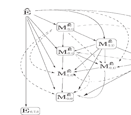
Figure 12: New fixed points obtained from $\widehat{E}$ by RG flows caused by meson operators. The arrows indicate allowed RG flows. Dashed lines are used just to make the relations easier to understand.

In this subsection we have explored flows caused by meson operators, starting from $\widehat{E}$. The new fixed points and the flows between them are summarized in figure 12.

5.3 Deformations of $M^{\widehat{E}}_{\ast}$ by $\mbox{Tr}X^{m}Y^{n}$

Take $M^{\widehat{E}}_{(3,0)}$ as an example. Relevant operators of the form $\Delta W^{\prime}={\rm Tr}X^{m}Y^{n}$ at the fixed point $M^{\widehat{E}}_{(3,0)}$, which has $W_{0}+\Delta W={\rm Tr}Y^{3}+\widetilde{Q}_{i}X^{3}Q^{i}$, are

$$\mbox{Tr}X^{5},\mbox{Tr}X^{3}Y,\mbox{Tr}X^{4},\mbox{Tr}X^{2}Y,\mbox{Tr}XY,\mbox{Tr}X^{2},~{}{\rm and}~{}\mbox{Tr}Y^{2},$$ (5.4)

where we listed only inequivalent deformations, using the chiral ring relation $Y^{2}\sim 0$ and the fact that the deformation by $\mbox{Tr}X^{3}$ is equivalent to the deformation by $\mbox{Tr}X^{2}Y$ by a change of variables. The first four deformations do not lead to an interacting fixed point, since none of the assumptions 1)-3) at the beginning of this subsection is consistent in the range of $x$ where $M^{\widehat{E}}_{(3,0)}$ exists. The remaining deformations $\mbox{Tr}X^{2}$, $\mbox{Tr}Y^{2}$ and $\mbox{Tr}XY$ are mass deformations. The deformation $\mbox{Tr}Y^{2}$ makes $Y$ massive, leading to the one-adjoint SQCD with the superpotential $\widetilde{Q}_{i}X^{3}Q^{i}$. This theory cannot be an interacting CFT because the assumption $R(\widetilde{Q}_{i}X^{3}Q^{i})=2$ is inconsistent with unitarity. The deformation $\mbox{Tr}XY$ makes both $X$ and $Y$ massive and leads to SQCD that does not have a stable vacuum in the range $x>1$. The $\mbox{Tr}X^{2}$ deformation deforms $M^{\widehat{E}}_{(3,0)}$ to the $A_{2}$ fixed point.

Relevant ${\rm Tr}X^{m}Y^{n}$ deformations of other fixed points of the form $M^{\widehat{E}}_{\ast}$ can be studied similarly. Most of them do not lead to an interacting fixed point. The exception is the mass deformation by ${\rm Tr}X^{2}$ of $M^{\widehat{E}}_{(m,0)},~{}m=1,2,3$ that leads to the $A_{2}$ theory.

6 Superpotential Deformations of $\widehat{A}$

Deformations by ${\rm Tr}X^{k+1},~{}k=2,3,...$ of the $\widehat{A}$ fixed point were considered in [7] and lead to the fixed points $A_{k}$. In this section, we consider deformations by other types of superpotential terms.

The $\widehat{A}$ theory is asymptotically free for $x>1/2$. The $R$ charges are obtained by $a$-maximization, taking into account the corrections due to the mesons hitting the unitarity bound. $R(Q)=:y(x)$ and $R(X)=(1-y(x))/x$ are monotonically decreasing functions of $x$ with asymptotics $R(Q)\sim 1-\frac{\sqrt{5}}{3}\simeq 0.244$ and $R(X)\sim\frac{4-\sqrt{3}}{3x}$ as $x\rightarrow\infty$ [7].

We are interested in relevant deformations constructed from mesons ${\mathcal{M}}_{l}\equiv\widetilde{Q}X^{l-1}Q$. Since no meson can have $R$ charge smaller than $2/3$, we consider a single meson or a product of two mesons: $\widetilde{Q}_{i}X^{l-1}Q^{i}$, $(\widetilde{Q}_{i}X^{l_{1}-1}Q^{j})(\widetilde{Q}_{i}X^{l_{2}-1}Q^{j})$ and $(\widetilde{Q}_{i}X^{l_{1}-1}Q^{i})(\widetilde{Q}_{j}X^{l_{2}-1}Q^{j})$. More than two mesons cannot give a relevant operator.

The deformation of $\widehat{A}$ by $\widetilde{Q}_{i}X^{l-1}Q^{i}$ does not lead to an interacting fixed point for $x>1/2$ as we now see. If $R(\widetilde{Q}_{i}X^{l-1}Q^{i})>2/3$ at $\widehat{A}$, the assumption that $R(\widetilde{Q}_{i}X^{l-1}Q^{i})=2$ at the potential new fixed point leads to the $R$ charges $R(X)=0$ and $R(Q)=1$ that are inconsistent with unitarity. If $\widetilde{Q}_{i}X^{l-1}Q^{i}$ hits the unitarity bound at $\widehat{A}$ and is decoupled, the term linear in a free field cannot give an interacting CFT. By the same argument we conclude that an operator of the type $\mbox{Tr}X^{a}(\widetilde{Q}_{i}X^{b}Q^{i})$ does not lead to a new CFT.

We fix $m\geq 0$ and consider deformations by $(\widetilde{Q}_{i}X^{l_{1}-1}Q^{j})(\widetilde{Q}_{i}X^{l_{2}-1}Q^{j})$ and $(\widetilde{Q}_{i}X^{l_{1}-1}Q^{i})(\widetilde{Q}_{j}X^{l_{2}-1}Q^{j})$ with $l_{1}+l_{2}-2=m$ altogether. Also we restrict ourselves to the deformations that do not contain free mesons. These deformations give rise to a manifold of fixed points, which we refer to as $M^{\widehat{A}}_{(4,m)}$, as discussed in the introduction. The $R$ charges at $M^{\widehat{A}}_{(4,m)}$ are $R(X)={2\over 4x-m}$ and $R(Q)={2x-m\over 4x-m}$. Both of them are positive in the range where the deformations are relevant. Some mesons violate the unitarity bound and get decoupled. If we denote by $a_{0}$ the central charge computed without the decoupled operators taken in to account, the correct central charge is modified to

$$a^{\widehat{A}}_{(4,m)}=a_{0}+{1\over 9}\sum_{l=1}^{\infty}\left[2-3R({\cal M}_{l})\right]^{2}\left[5-3R({\cal M}_{l})\right]\theta\left(m-{3\over 2}(l-1)-x\right),$$ (6.5)

where $\theta$ is the Heaviside step function. We checked that the $a$-theorem conjecture is satisfied under the flows $\widehat{A}\rightarrow M^{\widehat{A}}_{(4,m)}$ and $M^{\widehat{A}}_{(4,m)}\rightarrow M^{\widehat{A}}_{(4,m-1)}.$ See figure 13.

Figure 13: Left: The central charges at $\widehat{A}$ (dashed) and $M^{\widehat{A}}_{(4,3)}$ (solid). Right: The central charge at $M^{\widehat{A}}_{(4,m)}$ at $x=50$. It decreases under the flow $M^{\widehat{A}}_{(4,m)}\rightarrow M^{\widehat{A}}_{(4,m-1)}$.

The new fixed points and the flows between them are summarized in figure 14.

Figure 14: Flows from $\widehat{A}$ by mesonic deformations. There is no flow that goes between $A_{k}$ and the theory $M^{\widehat{A}}_{(4,m)}$ obtained by a mesonic deformation of $\widehat{A}$.

7 Superpotential Deformations of $\widehat{D}$

In this section, we consider mesonic deformations of $\widehat{D}$. Procedures we will use is the same as the ones in previous sections. Also the basic features are the similar to $A$-type, so we will simply show the results.

Using the chiral ring relations $\{X,Y\}=Y^{2}=0$ and the $R$ charges shown in [8] we obtain the following relevant mesonic deformations at $\widehat{D}$,

$$\left[\widetilde{Q}_{i}X^{k}Q^{i},~{}(\mbox{Tr}X^{a})\widetilde{Q}_{i}X^{b}Q^{i}\right],~{}\left[(\widetilde{Q}_{i}X^{l_{1}}Q^{i})(\widetilde{Q}_{j}X^{l_{2}}Q^{j}),~{}(\widetilde{Q}_{i}X^{l_{1}}Q^{j})(\widetilde{Q}_{j}X^{l_{2}}Q^{i})\right],$$ (7.6)

$$\left[\widetilde{Q}_{i}X^{l}YQ^{i},~{}(\mbox{Tr}X^{a})\widetilde{Q}_{i}X^{b}YQ^{i},\quad(\mbox{Tr}X^{a}Y)\widetilde{Q}_{i}X^{b}Q^{i}\right],$$ (7.7)

$$\left[(\widetilde{Q}_{i}X^{l_{1}}Q^{i})(\widetilde{Q}_{j}X^{l_{2}}YQ^{j}),~{}(\widetilde{Q}_{i}X^{l_{1}}Q^{j})(\widetilde{Q}_{j}X^{l_{2}}YQ^{i})\right],(\mbox{Tr}X^{a}Y)\widetilde{Q}_{i}X^{b}YQ^{i}.$$ (7.8)

Operators in $[...]$ give a single manifold of fixed points.

The deformation of $\widehat{D}$ by $\widetilde{Q}_{i}X^{l}Q^{i}$ does not lead to a new fixed point. This is because requiring that ${\rm Tr}XY^{2}$ and $\widetilde{Q}_{i}X^{l}Q^{i}$ have $R$ charge 2, we get $R(Q)=1,R(X)=0,R(Y)=1$, which are inconsistent with unitarity.

Deformations of $\widehat{D}$ by $(\widetilde{Q}_{i}X^{l_{1}}Q^{i})(\widetilde{Q}_{j}X^{l_{2}}Q^{j})$ and $(\widetilde{Q}_{i}X^{l_{1}}Q^{j})(\widetilde{Q}_{j}X^{l_{2}}Q^{i})$

The operators $(\widetilde{Q}_{i}X^{l_{1}}Q^{i})(\widetilde{Q}_{j}X^{l_{2}}Q^{j})$ and $(\widetilde{Q}_{i}X^{l_{1}}Q^{j})(\widetilde{Q}_{j}X^{l_{2}}Q^{i})$ with $l_{1}+l_{2}=k$ produce a manifold of fixed points that we call $M^{\widehat{D}}_{(1,m,0)}$. The $R$ charges are $R(Q)=\frac{x-k}{2x-k},R(X)=\frac{2}{2x-k},R(Y)=\frac{2x-k-1}{2x-k}$. We checked for $k\leq 5$ and $k\gg 1$ that $R(X)$ is positive in the region where the operator $(\widetilde{Q}X^{l_{1}}Q)(\widetilde{Q}X^{l_{2}}Q)$ are relevant. There are flows $M^{\widehat{D}}_{(1,k,0)}\rightarrow M^{\widehat{D}}_{(1,k-1,0)}$. We checked that the $a$-theorem is satisfied under this flow. See figure 15.

Figure 15: The central charge at $M^{\widehat{A}}_{(1,k,0)}(40)$.

Deformations of $\widehat{D}$ by $\widetilde{Q}_{i}X^{l}YQ^{i}$

The deformation of $\widehat{D}$ by $\widetilde{Q}_{i}X^{l}YQ^{i}$ leads to a fixed point that we call $M^{\widehat{D}}_{(0,l,1)}$. $X$ has a positive $R$ charge , and there is a flow $M^{\widehat{D}}_{(0,l,1)}\rightarrow M^{\widehat{D}}_{(0,l-1,1)}$. We checked that the $a$-theorem is satisfied here. Since the operators $(\mbox{Tr}X^{a})\widetilde{Q}_{i}X^{b}YQ^{i}$ and $(\mbox{Tr}X^{a}Y)\widetilde{Q}_{i}X^{b}Q^{i}$ with $a+b=k$ give the same beta function we regard these operators as the exactly marginal opetrators.

Deformations of $\widehat{D}$ by $(\widetilde{Q}_{i}X^{l_{1}}Q^{i})(\widetilde{Q}_{j}X^{l_{2}}YQ^{j})$ and $(\widetilde{Q}_{i}X^{l_{1}}Q^{j})(\widetilde{Q}_{j}X^{l_{2}}YQ^{i})$

$(\widetilde{Q}_{i}X^{l_{1}}Q^{i})(\widetilde{Q}_{j}X^{l_{2}}YQ^{j})$ and $(\widetilde{Q}_{i}X^{l_{1}}Q^{j})(\widetilde{Q}_{j}X^{l_{2}}YQ^{i})$ with $l_{1}+l_{2}=k$ for fixed $k$ give rise to a manifold of fixed points that we call $M^{\widehat{A}}_{(1,k,1)}$. The central charge is

$$a^{\widehat{D}}_{(k,1)}(x)=\frac{2\,x^{2}\,\left(2+152\,k^{2}+2\,x+35\,x^{2}-4\,k\,\left(1+38\,x\right)\right)}{{\left(1-4\,k+2\,x\right)}^{3}}.$$ (7.9)

Again we checked the positivity of $R(X)$. Thus there is a flow $M^{\widehat{D}}_{(1,k,1)}\rightarrow M^{\widehat{D}}_{(1,k-1,1)}$. We checked that the $a$-theorem is satisfied here.

Deformations of $\widehat{D}$ by $(\mbox{Tr}X^{a}Y)\widetilde{Q}_{j}X^{b}YQ^{j}$

Likewise $R$ charges are given as $R(X)={2\over x-k+1}$, $R(Y)={x-k\over x-k+1}$ and $R(Q)={1-k\over x-k+1}$. We checked positivity of $R(X)$ for $k\gg 1$ in the region where $(\mbox{Tr}X^{a}Y)\widetilde{Q}_{j}X^{b}YQ^{j}$ is relevant and $M^{\widehat{D}}_{(0,k,2)}$ $\to$ $M^{\widehat{D}}_{(0,k,2)}$. We checked a-theorem for several model with $k\leq 4$.

Finally let us comment on deformations of $M^{\widehat{D}}_{(0,m,1)}$ by ${\rm Tr}X^{m}Y^{n}$. Using the $R$ charges shown above we see there are several relevant operators of this type if we take $x$ to be large enough. However from the chiral ring relation some of operators are equivalent to certain mesonic deformations and only one type of deformations becomes independent, $\mbox{Tr}X^{k}$ with ${4m+3k-1\over 2}>x>{4m+k-1\over 2}$. If the superpotential $QX^{m}YQ$ is irrelevant under the flow, it drive the theory to $D_{k+1}$. Unfortunately in this case there appear infinite number of baryonic operators which hit the unitarity bound. Therefore we could not explicitly check if this flow occurs or not. From the results of $E$ and $A$-type results we expect that there is no flow between $D_{k+2}$ with mesonic type fixed points. All the RG flows driven by mesonic deformation are summarized in figure 16.

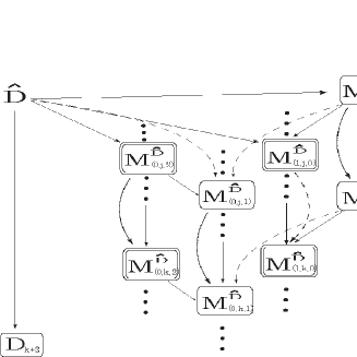
Figure 16: Flows driven by mesonic deformation of $\widehat{D}$.

8 Summary and Discussion

In this paper, we studied large classes of RG flows, triggered by either scalar expectation values or superpotential terms.

Sections 2 and 3 were devoted to Higgsing of the $D$- and $E$-type RG fixed points. As an example of Higgsing of a $D$-type theory, in section 2 we took the flow from $\widehat{D}$ to the model in [18], which breaks the gauge group as $U(N)\to U(N_{1})\times U(N_{2})$ and ends up with a superpotential constructed from bifundamental as well as adjoint fields. By exploiting the existence of a Seiberg duality for this model, we proposed a prescription, generalizing similar ones used in other cases, which determines the two-dimensional conformal window of the model, which is parameterized by $(x,y)=(N_{1}/N_{f},N_{2}/N_{f})$. We focused on the cases $k=3$ and $k\gg 1$, and determined the values of $(x,y)$, in the large $N$ limit eq.(1.2), at the corners of the conformal window. This allowed us do draw a picture of the two-dimensional conformal window in each of the $k=3$ and $k\gg 1$ cases (figure 4). In section 3 we considered Higgsing of $E$-type theories and studied the non-Abelian Coulomb phase of the model after Higgsing and checked the validity of the $a$-theorem. Compared with the RG flows triggered by superpotential deformations or gauge interactions, we still have little understanding of how the $a$-theorem works for Higgsing RG flows. Still, we have added more to the evidence supporting the conjectural $a$-theorem for the Higgsing RG flows.

In sections 4-7, we studied mesonic and monomial superpotential deformations of $ADE$-type fixed points. We explored a large number of new RG-fixed points and the RG-flows between them. All of the new RG-fixed points can be reached from $\widehat{O}$ by some superpotential deformations. We did not see any violation of the $a$-theorem. Also we pointed out that when we classify relevant operators by using the chiral ring relations, we need to consider a constant shift of a field separately though it is an example of a field redefinition.

We extended in many directions the classes of conformal fixed points obtained from a two-adjoint gauge theory with flavors. Our hope was that this would give a clue to understand the appearance of the $ADE$ classification, as explained in the introduction. Unfortunately, the mystery remains unsolved, and we feel that it is an interesting future direction.

Appendix A Perturbative Calculation

In this appendix we will check the existence of the RG fixed points $\widehat{M}$, $M^{\widehat{D}}_{(0,1)}$, $M^{\widehat{E}}_{10}$ and $M^{\widehat{E}}_{(0,1)}$ by perturbative calculations. Since we are interested in the large $N,N_{f}$ limit with fixed $x=N/N_{f}$, the perturbative region can be represented by $x\simeq 1+\epsilon$ with $0\leq\epsilon\ll 1$. The beta functions of gauge coupling and Yukawa interactions are listed in [24] up to two-loop order in perturbation. At one-loop order the superpotential deformations do not affect the gauge coupling beta function and as shown in [8] gauge coupling at the fixed point can be written as

$${g_{\ast}^{2}N_{c}\over 8\pi^{2}}\simeq{\epsilon\over 4}.$$ (A.10)

Below we will use show the beta functions of the RG fixed points $\widehat{M}$, $M^{\widehat{D}}_{(0,1)}$, $M^{\widehat{E}}_{10}$ and $M^{\widehat{E}}_{(0,1)}$ and check the existence.

$W=\lambda\widetilde{Q}XQ$ at the $\widehat{M}$ RG fixed point

From the formula $(2.10)$ in [24] we obtain the anomalous dimensions of the fields $Q$, $\widetilde{Q}$ and $X$ as follows:

$$\gamma(Q) = \gamma(\widetilde{Q})={\lambda^{2}\over 64\pi^{2}}N-{1\over 16\pi^{2}}g^{2}N$$

$$\gamma(X) = {\lambda^{2}N\over 64\pi^{2}}-{1\over 8\pi^{2}}g^{2}N$$ (A.11)

Plugging these into the beta function, we obtain

$$\beta(\lambda)={1\over 2}\lambda\left[\gamma(X)+2\gamma(Q)\right]={1\over 2}\lambda\left[3{\lambda^{2}\over 64\pi^{2}}N-{\epsilon\over 2}\right].$$ (A.12)

At the new RG fixed point, the coupling constant becomes

$$\lambda^{2}_{\ast}={32\pi^{2}\over 3N}\epsilon.$$ (A.13)

$W=\lambda_{1}\widetilde{Q}XQ+{1\over 6}\lambda_{2}\mbox{Tr}X^{3}$ at the $M^{\widehat{E}}_{(0,1)}$ RG fixed point

In the same way we examine $M^{\widehat{E}}_{(0,1)}$. The beta functions for the two coupling constants in the superpotential are

$$\beta(\lambda_{1}) = {1\over 2}\lambda_{1}(\gamma(X)+2\gamma(Q))={\lambda_{1}\over 2}\left[{3\lambda_{1}^{2}N+2\lambda_{2}^{2}d^{2}\over 64\pi^{2}}-{\epsilon\over 2}\right]$$

$$\beta(\lambda_{2}) = {3\over 2}\lambda_{2}\gamma(X)={3\over 2}\lambda_{2}\left[{\lambda_{1}^{2}N+2\lambda_{2}^{2}d^{2}\over 64\pi^{2}}-{\epsilon\over 4}\right].$$ (A.14)

Again the contribution of superpotential is negative and drive the theory to new RG fixed points where the coupling constants have the following values,

$${\lambda_{1}^{2}}_{\ast}={8\pi^{2}\epsilon\over N},\quad{\lambda_{2}^{2}}_{\ast}={4\pi^{2}\epsilon\over d^{2}}.$$ (A.15)

Here $d^{2}$ is defined by

$$d_{abc}d^{ebc}=d^{2}\delta_{a}^{e},\qquad{\rm where}\quad\ d^{abc}=\mbox{Tr}[T^{a}\{T^{b}T^{c}\}].$$ (A.16)

$W=\lambda_{1}\widetilde{Q}XQ+{1\over 6}\lambda_{2}\mbox{Tr}Y^{3}$ at the $M^{\widehat{E}}_{(1,0)}$ RG fixed point

We proceed to the calculation of beta function of $M^{\widehat{E}}_{(1,0)}$. In this case $\gamma(Q)$ and $\gamma(X)$ are the same as the ones for $\widehat{M}$ and althought $\gamma(Y)$ is diffrent.

$$\beta(\lambda_{1})={1\over 2}\lambda_{1}\left[{3\lambda^{2}_{1}\over 64\pi^{2}}N-{\epsilon\over 2}\right],\quad\beta(\lambda_{2})={2\over 3}\lambda_{2}\left[{\lambda_{2}^{2}d^{2}\over 32\pi^{2}}-{g^{2}N\over 8\pi^{2}}\right]$$ (A.17)

$${\lambda^{2}_{1}}_{\ast}={32\pi^{2}\over 3N}\epsilon,\quad{\lambda_{2}^{2}}_{\ast}={8\pi^{2}\over d^{2}}\epsilon.$$ (A.18)

$W=\lambda_{1}\widetilde{Q}XQ+{1\over 2}\lambda_{2}\mbox{Tr}X^{2}Y$ at the $M^{\widehat{D}}_{(0,1)}$ RG fixed point

Last one is $M^{\widehat{D}}_{(0,1)}$. In this case $\gamma(Q)$ is the same as the one for $\widehat{M}$. Plugging it into the formula for the beta function, we obtain

$$\beta(\lambda_{1})={\lambda_{1}\over 2}\left[{3\lambda_{1}^{2}N+4\lambda_{2}^{2}d^{2}\over 64\pi^{2}}-{\epsilon\over 2}\right],\qquad\beta(\lambda_{2})={\lambda_{2}\over 2}\left[{\lambda_{1}^{2}N+5\lambda_{2}^{2}d^{2}\over 32\pi^{2}}-{3\epsilon\over 4}\right].$$ (A.19)

At the new RG fixed point the coupling constants have values

$${\lambda^{2}_{1}}_{\ast}={64\pi^{2}\over 11N}\epsilon,\quad{\lambda_{2}^{2}}_{\ast}={40\pi^{2}\over 11d^{2}}\epsilon.$$ (A.20)

Appendix B Higgsing of $A$-type Fixed Points

We give a brief review of Higgsing of the $\widehat{A}$ theory studied in [7]. When the adjoint field $X$ acquires a vacuum expectation value,

$$\langle X\rangle={\rm diag}(\stackrel{{\scriptstyle N_{0}}}{{\overbrace{0,\cdots,0}}},\stackrel{{\scriptstyle N_{1}}}{{\overbrace{a_{1},\cdots,a_{1}}}},\cdots\stackrel{{\scriptstyle N_{n}}}{{\overbrace{a_{n},\cdots,a_{n}}}}),\qquad\sum_{i=0}^{n}N_{i}=N$$ (B.21)

the gauge group $SU(N)$ breaks into a product group $\prod SU(N_{i})$. Since bifundamental matter fields coming from the fluctuations of the original $X$ are eaten, the $SU(N_{i})$ factors do not interact with each other. Thus the theories become a product of several $\widehat{A}$ theories and do not provide new interacting CFT points.

Adding a mesonic superpotential $W=\widetilde{Q}X^{m}Q$ and considering Higgsing, can we obtain different kinds of non-trivial fixed points? Plugging (B.21) back into the superpotential we obtain the following superpotentials,

$$W=\widetilde{Q}_{0}X_{0}^{m}Q_{0}+\sum_{i=1}^{n}\sum_{k=0}^{m}(a_{i})^{k}\widetilde{Q}_{i}X_{i}^{m-k}Q_{i},$$ (B.22)

where we decomposed the original quark superfields $Q$ into $n+1$ subsectors $Q_{i}$, and $X_{i}$ is an adjoint superfield of $SU(N_{i})$ group. We omitted the flavor index of $Q_{i}$. In the subsectors with a nonzero vev, quark superfields $Q_{i}$ with $i=1,\cdots n$ are massive and thus are integrated out in the IR, although $Q_{0}$, being in the subsector with a vanishing vev, remains massless. The marginality of the first superpotential term gives $2R(Q_{0})+mR(X_{0})=2$ and the ABJ anomaly cancellation condition can be written as $N_{0}R(X_{0})+N_{f}R(Q_{0})=N_{f}$. Combining these two conditions we conclude that $R(X_{0})=0$, $R(Q_{0})=1$ and $a=0$. As in similar cases in the text, we conclude that there is no non-trivial fixed point.

What if we further add $\mbox{Tr}X^{k+1}$, namely Higgsing of the $A_{k+1}$ model? Again we assume the vev (B.21), after Higgsing, the adjoint superfields of $SU(N_{i})$ with $i=1,\cdots n$ have mass terms and are integrated out. Thus those subsectors are driven to the product of several copies of SQCD that does not have any non-trivial fixed point in the range $N/N_{f}>1$. On the other hand a subsector $SU(N_{0})$ has a superpotential term $\mbox{Tr}X_{0}^{k}$ which is the $A_{k+1}$ theory. Thus we conclude that Higgsing of the $A$-type theories (i.e., $\widehat{A}$ and $A_{k+1}$) does not lead to new interacting fixed points. This is in contrast with the $D$-type ($\widehat{D}$ and $D_{k+2}$) and $E$-type ($\widehat{E}$ and $E_{6,7,8}$) theories where there are several breaking patterns which drive the theory to new interacting fixed points.

Appendix C Undetermined Flow: $(\widetilde{Q}Q)^{2}$ deformation of $M_{(3,0)}^{\widehat{E}}$

Among the many RG flows we studied, there was one case where we could not determine which flow actually occurs. That is the deformation of $M^{\widehat{E}}_{(3,0)}$ by $\Delta W^{\prime}=\widetilde{Q}_{j}Q^{i}\widetilde{Q}_{i}Q^{j}$. The operator becomes relevant for $x>{15\over 4}$ although $M^{\widehat{E}}_{(3,0)}$ exists only in $x>40.8$. Hence we focus on the region where both conditions are satisfied.

First we study the case in which $R$ charges of $\mbox{Tr}Y^{3}$ and $\widetilde{Q}_{j}Q^{i}\widetilde{Q}_{i}Q^{j}$ are two, assuming that $\widetilde{Q}_{i}X^{3}Q^{i}$ is irrelevant under the RG-flow. $R$ charge at the fixed point can be given as $R(Y)={2\over 3}$, $R(X)={1\over 3}+{1\over 2x}$, and $R(Q)={1\over 2}$. There is no operator which violates the unitarity bound. With these $R$ charges let us check if operator $\widetilde{Q}_{i}X^{3}Q^{i}$ is irrelevant or not: $R(\widetilde{Q}_{i}X^{3}Q^{i})={2}+{3\over 2x}>2$. Thus there is not contradiction to our assumption. The $a$-theorem also satisfied in this flow.

Let us next consider the another possibility and assume that $\mbox{Tr}Y^{3}$ is irrelevant after the RG flow. In this case $R$ charges are given by $R(X)={1\over 3}$, $R(Y)={2\over 3}+{1\over 2x}$ and $R(Q)={1\over 2}$. We call this new fixed point $M^{(3,0)}_{(4,0,0)}$. $\mbox{Tr}Y^{3}$ is irrelevant after the flow: $R(\mbox{Tr}Y^{3})=2+{3\over 2x}>2$. The central charge $a$ in this fixed point also satisfies the $a$-theorem.

Which is the real flow? We expect that the latter one would actually occurs. As we see in the main text we obtain the RG-flows $M^{\widehat{E}}_{(3,0)}\to M^{\widehat{E}}_{(1,1)}$ and $M^{\widehat{E}}_{(1,1)}\to M^{\widehat{E}}_{(4,0,0)}$. So combining these two flows we can obtain an indirect flow from $M^{\widehat{E}}_{(3,0)}$ to $M^{\widehat{E}}_{(4,0,0)}$. On the other hand we can not reach $M^{(3,0)}_{(4,0,0)}$ from another RG-fixed points obtained in the main text. Therefore it is plausible that the RG flow $M^{\widehat{E}}_{(3,0)}\to M^{\widehat{E}}_{(1,1)}$ occurs.

References

- [1] K. Intriligator and B. Wecht, “The exact superconformal R-symmetry maximizes a,” Nucl. Phys. B 667, 183 (2003) [arXiv:hep-th/0304128].
- [2] D. Martelli, J. Sparks and S. T. Yau, arXiv:hep-th/0503183.
- [3] Y. Tachikawa, “Five-dimensional supergravity dual of a-maximization,” arXiv:hep-th/0507057.
- [4] E. Barnes, E. Gorbatov, K. Intriligator, M. Sudano and J. Wright, “The exact superconformal R-symmetry minimizes tau(RR),” arXiv:hep-th/0507137.
- [5] E. Barnes, E. Gorbatov, K. Intriligator and J. Wright, “Current correlators and AdS/CFT geometry,” arXiv:hep-th/0507146.
- [6] J. L. Cardy, “Is There A C Theorem In Four-Dimensions?” Phys. Lett. B 215, 749 (1988).
- [7] D. Kutasov, A. Parnachev and D. A. Sahakyan, “Central charges and U(1)R symmetries in N = 1 super Yang-Mills,” JHEP 0311, 013 (2003) [arXiv:hep-th/0308071].
- [8] K. Intriligator and B. Wecht, “RG fixed points and flows in SQCD with adjoints,” Nucl. Phys. B 677, 223 (2004) [arXiv:hep-th/0309201].
- [9] E. Barnes, K. Intriligator, B. Wecht and J. Wright, “Evidence for the strongest version of the 4d a-theorem, via a-maximization along RG flows,” arXiv:hep-th/0408156.
- [10] D. Kutasov, “New results on the ’a-theorem’ in four dimensional supersymmetric field theory,” arXiv:hep-th/0312098.
- [11] V.I. Arnold, S.M. Gusein-Zade and A.N. Varchenko, Singularities of Differentiable Maps volumes 1 and 2, Birkhauser (1985), and references therein.
- [12] D. Kutasov and A. Schwimmer, “Lagrange multipliers and couplings in supersymmetric field theory,” arXiv:hep-th/0409029.
- [13] F. Cachazo, S. Katz and C. Vafa, “Geometric transitions and N = 1 quiver theories,” arXiv:hep-th/0108120.
- [14] R. G. Leigh and M. J. Strassler, “Exactly marginal operators and duality in four-dimensional N=1 supersymmetric gauge theory,” Nucl. Phys. B 447, 95 (1995) [arXiv:hep-th/9503121].
- [15] E. Barnes, K. Intriligator, B. Wecht and J. Wright, “N = 1 RG flows, product groups, and a-maximization,” Nucl. Phys. B 716, 33 (2005) [arXiv:hep-th/0502049].
- [16] D. Anselmi, J. Erlich, D. Z. Freedman and A. A. Johansen, “Positivity constraints on anomalies in supersymmetric gauge theories,” Phys. Rev. D 57, 7570 (1998) [arXiv:hep-th/9711035].
- [17] D. Anselmi, D. Z. Freedman, M. T. Grisaru and A. A. Johansen, “Nonperturbative formulas for central functions of supersymmetric gauge theories,” Nucl. Phys. B 526, 543 (1998) [arXiv:hep-th/9708042].
- [18] J. H. Brodie, “Duality in supersymmetric SU(N/c) gauge theory with two adjoint chiral superfields,” Nucl. Phys. B 478, 123 (1996) [arXiv:hep-th/9605232].
- [19] N. Seiberg, “Electric - magnetic duality in supersymmetric nonAbelian gauge theories,”Nucl. Phys. B 435, 129 (1995)[arXiv:hep-th/9411149].
- [20] K. A. Intriligator, R. G. Leigh and M. J. Strassler, “New examples of duality in chiral and nonchiral supersymmetric gauge theories,” Nucl. Phys. B 456, 567 (1995) [arXiv:hep-th/9506148].
- [21] Carina Curto, “Matrix Model Superpotentials and Calabi-Yau Spaces: an ADE Classification,’ [arXiv:math.AG/0505111].
- [22] D. Kutasov, “A Comment on duality in N=1 supersymmetric nonAbelian gauge theories,” Phys. Lett. B 351, 230 (1995) [arXiv:hep-th/9503086].
- [23] D. Kutasov and A. Schwimmer, “On duality in supersymmetric Yang-Mills theory,” Phys. Lett. B 354, 315 (1995) [arXiv:hep-th/9505004].
- [24] S. P. Martin and M. T. Vaughn, “Two loop renormalization group equations for soft supersymmetry breaking couplings,” Phys. Rev. D 50, 2282 (1994) [arXiv:hep-ph/9311340].