Evolution of a Self-interacting Scalar Field in the Spacetime of a Higher Dimensional Black Hole

Abstract

In the spacetime of n-dimensional static charged black hole we examine the mechanism by which the self-interacting scalar hair decay. It is turned out that the intermediate asymptotic behaviour of the self-interacting scalar field is determined by an oscillatory inverse power law. We confirm our results by numerical calculations.

I Introduction

The problem of the late-time behaviour of various fields in the spacetime of a collapsing body is well established (both analytically and numerically). It plays an important role in black hole’s physics. Black hole radiates away everything that it can. This phenomenon happens regardless of details of the collapse or the structure and properties of the collapsing body. The resultant black hole can be described only by few parameters such as mass, charge and angular momentum and due to the Wheeler’s metamorphic dictum black holes have no hair (see for the vast amount of references concerning this problem [2]). Therefore it is interesting to investigate how these hair loss proceed dynamically.

The neutral external perturbations were first studied in Ref.[3]. It was found that the late-time behavior is dominated by the factor $t^{-(2l+3)}$, for each multipole moment $l$. On the other hand, the decay-rate along null infinity and along the future event horizon was governed by the power laws $u^{-(l+2)}$ and $v^{-(l+3)}$, where $u$ and $v$ were the outgoing Eddington-Finkelstein (ED) and ingoing ED coordinates [4]. The scalar perturbations on Reissner-Nordtröm (RN) background for the case when $\mid Q\mid<M$ has the following dependence on time $t^{-(2l+2)}$, while for $\mid Q\mid=M$ the late-time behavior at fixed $r$ is governed by $t^{-(l+2)}$ [5].

It turns out that a charged hair decayed slower than a neutral one [6]-[8], while the late-time tails in gravitational collapse of a self-interacting (SI) fields in the background of Schwarzschild solution was reported by Burko [9] and in RN solution at intermediate late-time was considered in Ref.[10]. At intermediate late-time for small mass $m$ the decay was dominated by the oscillatory inverse power tails $t^{-(l+3/2)}\sin(mt)$. This analytic prediction was verified at intermediate times, where $mM\leq mt\leq 1/(mM)^{2}$. In Ref.[11] the nearly extreme RN spacetime was considered and it was found analytically that the inverse power law behavior of the dominant asymptotic tail is of the form $t^{-5/6}\sin(mt)$, independent of $l$. The asymptotic tail behaviour of SI scalar field was also studied in Schwarzschild spacetime [12]. The oscillatory tail of scalar field has the decay rate of $t^{-5/6}$ at asymptotically late time. The power-law tails in the evolution of a charged massless scalar field around a fixed background of dilaton black hole was studied in Ref.[13], while the case of a self-interacting scalar field was elaborated in [14].

Nowadays it seems that that it is impossible to construct a consistent theory unifying gravity with other forces in Nature in four dimensions. The no-hair theorem for $n$-dimensional static black holes is quite well established [15]. So it will be not amiss to ask about the mechanism of decaying black hole hair in higher dimensional static black hole case. The evolution of massless scalar field in the $n$-dimensional Schwarzshild spacetime was determined in Ref.[16]. It was found that for odd dimensional spacetime the field decay had a power falloff like $t^{-(2l+n-2)}$, where $n$ is the dimension of the spacetime. This tail was independent of the presence of the black hole. For even dimensions the late-time behaviour is also in the power law form but in this case it is due to the presence of black hole $t^{-(2l+3n-8)}$. Gravitational perturbations of maximally symmetric black hole spacetime in higher dimensions were studied by Kodama et al. [17], while gravitational quasi-normal radiation of higher dimensional black holes was elaborated in [18].

In our work we shall consider and discuss the SI scalar field behaviour in the spacetime of $n$-dimensional static charged black hole. In Sec.II we gave the analytic arguments concerning the intermediate behavior of SI scalar field in the background of the considered black hole. Then, in Sec.III we treated the problem numerically and check our analytical considerations. We conclude our investigations in Sec.IV.

II Massive scalar fields in n-dimensional spherically symmetric spacetime

In our paper we shall investigate the evolution of SI (massive) scalar field $\tilde{\psi}$ in a fixed spacetime of a static electrically charged $n$-dimensional black hole. The wave equation for the field is given in the form as follows:

$${}{}^{(n)}\nabla_{\mu}{}{}^{(n)}\nabla^{\mu}\tilde{\psi}-m^{2}\tilde{\psi}^{2}=0.$$ (1)

where $m$ is assumed to be real.

The metric of the external gravitational field will be given by the static, spherically symmetric solution of equations of motion derived from the action written as

$$S=\int d^{n}x\sqrt{-{}{}^{(n)}g}\left[{}{}^{(n)}R-F_{(n-2)}^{2}\right],$$ (2)

where we denoted the generalized $(n-2)$-gauge form $F_{\mu_{1}\dots\mu_{n-2}}$ by the expression $F_{(n-2)}=dA_{(n-3)}$. Further, we assume that we have to do with the only one nontrivial electric component of the $(n-2)$-gauge form as $A_{01\dots n-2}=\phi(x)$. The metric of the spherically symmetric charged static $n$-dimensional black hole implies

$$ds^{2}=-\bigg{(}1-{2M\over r^{n-3}}+{Q^{2}\over r^{2n-6}}\bigg{)}dt^{2}+{dr^{2}\over\bigg{(}1-{2M\over r^{n-3}}+{Q^{2}\over r^{2n-6}}\bigg{)}}+r^{2}d\Omega_{n-2}^{2},$$ (3)

where $d\Omega_{n-2}^{2}$ is the line element of the unit $S^{n-2}$ sphere. Next, we define the tortoise coordinates $y$ as

$$dy={dr\over\bigg{(}1-{2M\over r^{n-3}}+{Q^{2}\over r^{2n-6}}\bigg{)}}.$$ (4)

Thus, the metric (3) can be rewritten in the form as

$$ds^{2}=\bigg{(}1-{2M\over r^{n-3}}+{Q^{2}\over r^{2n-6}}\bigg{)}\bigg{[}-dt^{2}+dy^{2}\bigg{]}+r^{2}d\Omega_{n-2}^{2}.$$ (5)

In the spherical background each of the multipole of perturbation field evolves separetly. Because of the fact that the scalar field is of the form

$$\tilde{\psi}=\sum_{l,m}{1\over r^{{n-2\over 2}}}\psi_{m}^{l}(t,r)Y_{l}^{m}(\theta,\phi),$$ (6)

where $Y_{l}^{m}$ is a scalar spherical harmonics on the unit $(n-2)$-sphere and $m$ denotes a set of $(n-3)$ integers $(m_{1}\dots m_{n-3})$ satisfying $l\geq m_{n-3}\geq\dots\geq m_{2}\geq\mid m_{1}\mid$. In the process of this one has the following equations of motion for each multipole moment

$$\psi_{,tt}-\psi_{,yy}+V\psi=0.$$ (7)

The potential $V$ implies

$$V=f^{2}(r)\bigg{[}\bigg{(}{n-2\over 2}\bigg{)}{1\over r^{{n-2\over 2}}}{d\over dr}\bigg{(}r^{{n\over 2}-2}~{}f^{2}(r)\bigg{)}+{l(l+n-3)\over r^{2}}+m^{2}\bigg{]},$$ (8)

where $f^{2}(r)=1-{2M\over r^{n-3}}+{Q^{2}\over r^{2n-6}}$.

In order to analyze the time evolution of SI scalar field in the background of the considered black hole we shall use the spectral decomposition method [19]. The time evolution of SI scalar field may be written in the following form:

$$\psi(y,t)=\int dy^{\prime}\bigg{[}G(y,y^{\prime};t)\psi_{t}(y^{\prime},0)+G_{t}(y,y^{\prime};t)\psi(y^{\prime},0)\bigg{]},$$ (9)

for $t>0$, where the Green’s function $G(y,y^{\prime};t)$ is given by

$$\bigg{[}{\partial^{2}\over\partial t^{2}}-{\partial^{2}\over\partial y^{2}}+V\bigg{]}G(y,y^{\prime};t)=\delta(t)\delta(y-y^{\prime}).$$ (10)

Our main task will be to find the black hole Green function so in the first step we reduce equation (10) to an ordinary differential equation. To do it one can use the Fourier transform [20] $\tilde{G}(y,y^{\prime};\omega)=\int_{0^{-}}^{\infty}dtG(y,y^{\prime};t)e^{i\omega t}$. This Fourier’s transform is well defined for $Im~{}\omega\geq 0$, while the corresponding inverse transform yields

$$G(y,y^{\prime};t)={1\over 2\pi}\int_{-\infty+i\epsilon}^{\infty+i\epsilon}d\omega~{}\tilde{G}(y,y^{\prime};\omega)e^{-i\omega t},$$ (11)

for some positive number $\epsilon$. The Fourier’s component of the Green’s function $\tilde{G}(y,y^{\prime};\omega)$ can be written in terms of two linearly independent solutions for homogeneous equation as

$$\bigg{(}{d^{2}\over dy^{2}}+\omega^{2}-V\bigg{)}\psi_{i}=0,\qquad i=1,2,$$ (12)

The boundary conditions for $\psi_{i}$ are described by purely ingoing waves crossing the outer horizon $H_{+}$ of the $n$-dimensional static charged black hole $\psi_{1}\simeq e^{-i\omega y}$ as $y\rightarrow-\infty$ while $\psi_{2}$ should be damped expotentially at $i_{+}$, namely $\psi_{2}\simeq e^{-\sqrt{\omega^{2}-m^{2}}y}$ at $y\rightarrow\infty$.

In order to find $\psi_{i}$ we consider the wave Eq.(12) of SI scalar field and introduce an auxiliary variable $\xi$ in such a way that $\xi=f(r)\psi$. So in terms of $\xi$ relation (12) can be written as follows:

$${d^{2}\xi\over dr^{2}}-{f(r)_{,rr}\over f(r)}\xi++{\omega^{2}\xi\over f^{4}(r)}-{\xi\over f^{2}(r)}\bigg{[}\bigg{(}{n-2\over 2}\bigg{)}{1\over r^{{n-2\over 2}}}{d\over dr}\bigg{(}r^{{n\over 2}-2}~{}f^{2}(r)\bigg{)}+{l(l+n-3)\over r^{2}}+m^{2}\bigg{]}.$$ (13)

Further on, we expand Eq.(13) in power series of ${M\over r^{n-3}}$ and ${Q\over r^{n-3}}$, neglecting terms of order ${\cal O}\bigg{(}({\alpha\over r^{n-3}})^{2}\bigg{)}$. Then, we arrive at the following expression:

$${d^{2}\xi\over dr^{2}}+\bigg{[}\omega^{2}-m^{2}+{4M\omega^{2}-2Mm^{2}\over r^{n-3}}-{\nu(\nu+1)\over r^{2}}\bigg{]}\xi=0,$$ (14)

where $\nu=l-2+{n\over 2}$.
If one further assumes that the observer and the initial data are in the region where $r^{n-3}\ll{M\over(Mm)^{2}}$ and one shall be interested in the intermediate asymptotic behavior of SI scalar field $r^{n-3}\ll t\ll{M\over(Mm)^{2}}$, then we get

$${d^{2}\xi\over dr^{2}}+\bigg{[}\omega^{2}-m^{2}-{\nu(\nu+1)\over r^{2}}\bigg{]}\xi=0.$$ (15)

As in four-dimensional case the scalar field perturbations on $n$-dimensional charged static black hole background does not depend on the spacetime parameters such as $M$ and $Q$. The perturbations in question depend on the scalar field parameter (mass of the field).

The same procedure as described in Ref.[10] leads us to the solution of the relation (15) (we refer the readers to this work). Thus, in our case the intermediate asymptotic behaviour of the SI field at fixed radius has the form

$$\psi\sim t^{-(l+{n\over 2}-{1\over 2})},$$ (16)

while the intermediate behaviour of SI fields at the outer horizon $H_{+}$ is dominated by an oscillatory power law tails of the form as follows:

$$\psi\sim v^{-(l+{n\over 2}-{1\over 2})}\sin(mt).$$ (17)

In the next section we check our predictions numerically for various dimensions of the background spacetime.

III NUMERICAL RESULTS

We numerically analyzed Eq. (7) using method described in [4]. We transformed Eq. (7) into $(u,v)$ coordinates

$$4\psi_{,uv}+V\psi=0,$$ (18)

and solved it on uniformly spaced grid using explicit difference scheme. As was pointed out previously the late time evolution of a massive field is independent of the form of the initial data. In order to perform our calculation we start with a Gaussian pulse of the form as follows:

$$\psi(u=0,v)=A\exp\left(-{(v-v_{0})^{2}\over\sigma^{2}}\right)$$ (19)

Because of the linearity of the relation (7) one has freedom in choosing the value of the amplitude $A$. For our purpose we fix it as $A=1$. The rest of the initial field profile parameters we take as $v_{0}=50$ and $\sigma=2$.
We shall set the mass of SI scalar field equal to $m=0.01$ and the mass and charge of the black hole respectively equal to $M=0.5$, $Q=0.45$. First, we shall study the evolution of $\psi$ on the future timelike infinity $i_{+}$. In our calculations we approximate this situation by the field at fixed radius $y=50$. The numerical results for $l=0$ and different spacetime dimensions $n=4,5,6$ are shown in Fig. 1. Initially the evolution is determined by the prompt contribution and quasinormal ringing. However, then with the passage of time a definite oscillatory power-law fall off appears to be manifest. We obtained the power-law exponents $-1.51$, $-2.03$, and $-2.53$ for $n=4,5,6$, respectively. These values are to be compared with the analytically predicted ones equal respectively to $-1.5$, $-2.0$, and $-2.5$. Thus, the agreement between numerical calculations and analytically predicted values is excellent. For the four-dimensional spacetime we get the same result as obtained in Ref.[10]. The period of the oscillations is $T=\pi/m\simeq 314.5\pm 0.5$ to within $0.3\%$ for all curves. Both values of power-law exponents and period of oscillation are in perfect agreement with the analytical prediction.
Then, the evolution of the SI scalar field on the black hole future horizon $H_{+}$ (approximated by $\psi(u=10^{4},t)$), as a function of $v$ for different space dimensionality $n=4,5,6$ was studied. Calculation parameters are: $l=0$, $M=0.5$, $Q=0.45$, and $m=0.01$. The power-law exponents and the period of the oscillations are the same as in Fig. 1.
Next, we take into consideration the dependence of SI scalar field on the multiple index. We studied the evolution of the field $\psi$ on the future timelike infinity $i_{+}$ as a function of $t$ for different multipoles $l=0,1$ and $2$ in five-dimensional spacetime. The obtained power-law exponents are as follows: $-2.03$, and $-3.03$, and $-4.04$ for $l=0,1,2$. According to relation (16) these exponents are equal to $-2.0$, $-3.0$, and $-4.0$, in perfect agreement with numerical calculations. The period of the oscillations is $T=\pi/m\simeq 314.5$ to within $1\%$ for all curves, in agreement with the predicted value. The results are depicted in Fig. 3. The same calculations were conducted for six-dimensional spacetime (Fig. 4), where the power-law exponents are $-2.53$, and $-3.53$, and $-4.53$ for $l=0,1,2$, respectively. Due to Eq.(16) for six-dimensional spacetime they have the values: $-2.5$, $-3.5$, and $-4.5$. Those values are also in agreement with numerical calculations. The period of the oscillations is $T=\pi/m\simeq 314.5$ to within $3\%$ (for the worst case of $l=2$).
We also studied numerically the late-time behaviour of SI on black hole in five-dimensional spacetime, for the field mass $m=0.05$ (see Fig. 5). We investigated the behaviour on future timelike infinity and on black hole future horizon. The period of oscillation was $T=63.0$ to within $0.8\%$. The field’s amplitude decays in agreement with the no-hair theorem due to the power-law fall off, contrary to the four-dimensional case where one has the decay rate slower than any power-law. In six-dimensional case ( Fig. 6) the behaviour of SI scalar fields is the same, with the period of oscillation equal to $T=63.0$ to within $0.8\%$. The slope of the curve is equal to $-2.5$.
We also investigated the late-time behaviour on future timelike infinity in five-dimensional spacetime of static charged black hole for different masses of the scalar field Fig. 7. The decay rates have the form of the power-law fall-off with the slope equal to $-2.0$. The same studies were conducted in six-dimensional spacetime with the similar results Fig. 8, i.e., for various masses of SI scalar fields we obtained power-law fall off with the slope of the curve equal to $-2.5$.

IV Conclusions

We have elaborated analytically the intermediate behaviour of SI scalar fields in the background of static charged $n$-dimensional black hole. It turned out that the intermediate asymptotic behaviour did not depend on the spacetime parameters as $M$, $Q$ but only on the mass of SI scalar field. In other words, considering the SI scalar field perturbations one can neglect the backscattering from the asymptotically far regions at intermediate times. We check our analytical calculations by numerical ones and obtained excellent agreement with analytically predicted values. Numerical studies of the late-time behaviour of SI scalar fields on the future timelike infinity and on the future black hole horizon reveal the fact of the power-law decay (contrary to the four-dimensional case where one has to do with the slower than any power-law decay). The same type of behaviour was obtained for various masses of SI scalar fields in $n=5,6$ spacetime. This type of behaviour should be checked analytically, but due to the tremendous difficulties in solving differential equations is almost intractable. We hope to return to this problem elsewhere.

Acknowledgements:
M.R. was supported in part by KBN grant 1 P03B 049 29.

FIG. 1.: Evolution of the field $|\psi|$ on the future timelike infinity $i_{+}$ (approximated by $\psi(y=50,t)$) as a function of t for different space dimensionality $n=4,5,6$ (curves from top to bottom, respectively). Calculation parameters are: $l=0$, $M=0.5$, $Q=0.45$, and $m=0.01$. The power-law exponents are $-1.51$, $-2.03$, and $-2.53$ for $n=4,5,6$, respectively. The period of the oscillations is $T=\pi/m\simeq 314.5\pm 0.5$ to within $0.3\%$ for all curves.

FIG. 2.: Evolution of the field $|\psi|$ on the black hole future horizon $H_{+}$ (approximated by $\psi(u=10^{4},t)$) as a function of $v$ for different spacetime dimensionality $n=4,5,6$ (curves from top to bottom, respectively). Calculation parameters are: $l=0$, $M=0.5$, $Q=0.45$, and $m=0.01$. The power-law exponents and the period of the oscillations are the same as in Fig. 1.

FIG. 3.: Evolution of the field $|\psi|$ on the future timelike infinity $i_{+}$ (approximated by $\psi(y=50,t)$) as a function of t for different multipoles $l=0,1$ and $2$ (curves from top to bottom, respectively) and $n=5$. The power-law exponents are $-2.03$, and $-3.03$, and $-4.04$ for $l=0,1,2$, respectively. The period of the oscillations is $T=\pi/m\simeq 314.5$ to within $1\%$ for all curves. The rest of the parameters are the same as in Fig. 1.

FIG. 4.: Evolution of the field $|\psi|$ on the future timelike infinity $i_{+}$ (approximated by $\psi(y=50,t)$) as a function of t for different multipoles $l=0,1$ and $2$ (curves from top to bottom, respectively) and $n=6$. The power-law exponents are $-2.53$, and $-3.53$, and $-4.53$ for $l=0,1,2$, respectively. The period of the oscillations is $T=\pi/m\simeq 314.5$ to within $3\%$ (for the worst case of $l=2$). The initial data are those of Fig. 1.

FIG. 5.: Late-time behaviour of the field $|\psi|$ on black hole for $n=5$. Only maxima of the oscillations are shown. The mass of the field is $m=0.05$. The upper curve represents the field on future timelike infinity $i_{+}$ ($\psi(y=50)$) as a function of time $t$. Bottom curve is the field on the black hole future horizon $H_{+}$ ($\psi(u=2\times 10^{4}$) as a function of $v$. The period of the oscillations is $T=\pi/m\simeq 63.0$ to within $0.8\%$. The thin dashed lines have slopes equal to $-2.0$. The rest of the parameters are the same as in Fig. 1.

FIG. 6.: Late time behaviour of the field $|\psi|$ on black hole for $n=6$. Only maxima of the oscillations are shown. The mass of the field is $m=0.05$. The upper curve represents the field on future timelike infinity $i_{+}$ ($\psi(y=50)$) as a function of time $t$. Bottom curve is the field on the black hole future horizon $H_{+}$ ($\psi(u=2\times 10^{4}$) as a function of $v$. The period of the oscillations is $T=\pi/m\simeq 63.0$ to within $0.8\%$. The thin dashed lines have slopes equal to $-2.5$. The rest of the parameters are the same as in Fig. 1.

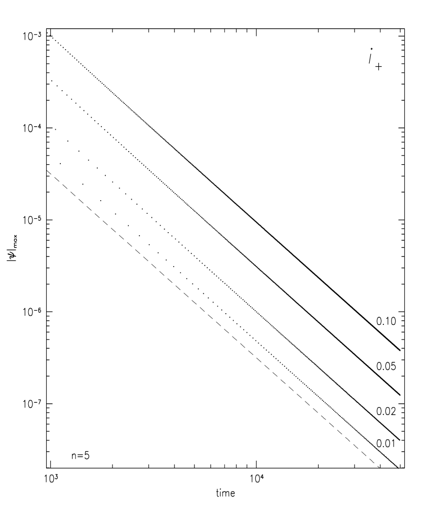
FIG. 7.: Late-time behaviour of the field $|\psi|_{max}$ at future timelike infinity on black hole for $n=5$ and for different masses $m$. The dashed line has slope equal to $-2.0$. The initial data are those of Fig. 1.

FIG. 8.: Late-time behaviour of the field $|\psi|_{max}$ at future timelike infinity on black hole for $n=6$ and for different masses $m$. The dashed line has slope equal to $-2.5$. The rest of the parameters are the same as in Fig. 1.

REFERENCES

- [1]
-
[2]
M.Heusler, Black Holes Uniqueness Theorems
(Cambridge University Press, Cambridge, England, 1996),
K.S.Thorne, Black Holes and Time Warps (W.W.Norton and Company, New York, 1994),
P.O.Mazur, Black Hole Uniqueness Theorem hep-th 0101012 (2001). - [3] R.H.Price, Phys. Rev. D 5, 2419 (1972).
- [4] C.Gundlach, R.H.Price and J.Pullin, Phys. Rev. D 49, 883 (1994).
- [5] J.Bicak, Gen. Rel. Grav. 3, 331 (1972).
- [6] S.Hod and T.Piran, Phys. Rev. D 58, 024017 (1998).
- [7] S.Hod and T.Piran, Phys. Rev. D 58, 024018 (1998).
- [8] S.Hod and T.Piran, Phys. Rev. D 58, 024019 (1998).
- [9] L.M.Burko, Abstracts of plenary taks and contributed papers, 15th International Conference on General Relativity and Gravitation, Pune, 1997, p.143, unpublished.
- [10] S.Hod and T.Piran, Phys. Rev. D 58, 044018 (1998).
- [11] H.Koyama and A.Tomimatsu, Phys. Rev. D 63, 064032 (2001).
- [12] H.Koyama and A.Tomimatsu, Phys. Rev. D 64, 044014 (2001).
- [13] R.Moderski and M.Rogatko, Phys. Rev. D 63, 084014 (2001).
- [14] R.Moderski and M.Rogatko, Phys. Rev. D 64, 044024 (2001).
-
[15]
G.W.Gibbons, D.Ida and T.Shiromizu, Prog. Theor. Phys. Suppl. 148, 284 (2003),
G.W.Gibbons, D.Ida and T.Shiromizu, Phys. Rev. Lett. 89, 041101 (2002),
G.W.Gibbons, D.Ida and T.Shiromizu, Phys. Rev. D 66, 044010 (2002),
M.Rogatko, Class. Quantum Grav. 19, L151 (2002),
M.Rogatko, Phys. Rev. D 67, 084025 (2003),
M.Rogatko, Phys. Rev. D 70, 044023 (2004),
M.Rogatko, Phys. Rev. D 71, 024031 (2005). - [16] V.Cardoso, S.Yoshida and O.J.C.Dias, Phys. Rev. D 68, 061503 (2003).
- [17] H.Kodama and A.Ishibashi, Prog. Theor. Phys. 110, 701 (2003).
- [18] R.A.Konoplya, Phys. Rev. D 68, 124017 (2003).
- [19] E.W.Leaver, Phys. Rev. D 34, 384 (1986).
- [20] N.Anderson, Phys. Rev. D 51, 353 (1995).