T-Duality and the Spectrum of Gravitational Waves

Abstract

In the inflationary universe scenario, the physical wavelength of cosmological fluctuation modes which are currently probed in observations was shorter than the Hubble radius, and in fact shorter than the Planck and string lengths, at the beginning of the period of inflation. Thus, during the early stages of evolution, the fluctuations are subject to Planck scale physics. In the context of an inflationary cosmological background, we examine the signatures of a specific modified dispersion relation motivated by the T-duality symmetry of string theory on the power spectrum of gravitational waves. The modified dispersion relation is extracted from the asymptotic limit of the string center of mass propagator.

I Introduction

The inflationary universe acts as a microscope which allows us, by means of cosmological observations performed today, to probe scales which at the beginning of the period of inflation were sub-Hubble (i.e. the wavelength was smaller than the Hubble radius), and in fact sub-Planckian (wavelength smaller than the Planck scale) RHBrev . This is possible since during the period of inflation (which we for concreteness take to be almost exponential) the physical wavelength of fixed perturbation modes increases exponentially, whereas the Hubble radius remains approximately constant. Thus, in principle, it is possible to probe Planck-scale or string-scale physics using current observations.

Crucial to the study of trans-Planckian effects on current cosmological observations is the ability to track the cosmological fluctuations from the earliest times and smallest scales to late times. Signatures of trans-Planckian physics then emerge via encoding the new physics which is effective at the Planck scale on the initial conditions and early evolution of the linearized fluctuations. This program was initially carried out Jerome1 ; Niemeyer making use of ad-hoc modified dispersion relations for the cosmological perturbations. These dispersion relations are linear (i.e. the usual ones) for physical wavenumbers smaller than a cutoff value which corresponds to the energy scale of the new physics, and deviates for larger wavenumbers. This approach has the advantage that it is easily computationally tractable. It was shown Jerome1 that observable effects are possible provided that the dispersion relation violates the adiabaticity condition, i.e. that the early evolution of the fluctuations is non-adiabatic from the point of view of the evolution which would have been obtained had the dispersion relation been the un-modified one. There are some constraints on the magnitude of trans-Planckian effects which come from back-reaction analyses Jerome2 , but these are less severe than initially conjectured in Tanaka ; Starob .

There are other approaches to studying the possible imprints of trans-Planckian physics on cosmological observations. In a “minimal” approach, initial conditions on the fluctuations are imposed not at some early initial time which is the same for all wavenumbers, but for each wavenumber at the time when the corresponding wavelength equals the scale of the new physics minimal . There are approaches which attempt to include crucial features of candidate theories of quantum gravity, e.g. via space-space uncertainty relations Columbia , space-time uncertainty relations Ho , Q-deformed structures Sera , and minimal length effects Kempf . Analyses based on an effective field theory approach have also been performed Cliff (see Jerome4 for a review and a more complete list of references).

In this paper we work under the hypothesis that superstring theory is the correct description of physics on the smallest length scales. A key feature which distinguishes string theory from point particle-based quantum field theory is the new symmetry of T-duality Tduality . We will explain this symmetry in the context of a theory with closed strings only, although the symmetry extends to theories with open strings Pol ; Boehm . Let us assume that each spatial direction is a torus with radius $R$. Closed strings have various degrees of freedom: momentum modes which correspond to the center of mass motion of the strings and whose energies are quantized in units of $1/R$ (setting the string length equal to 1 for this discussion), oscillatory modes which correspond to wiggles of the strings and whose energies are independent of $R$, and winding modes which count the number of times the string winds the torus, whose energies are quantized in units of $R$.

The string mass spectrum is

$$M^{2}\,=\,\frac{n^{2}}{R^{2}}+w^{2}R^{2}+2\left(\tilde{N^{\bot}}+N^{\bot}-2\right)$$ (1)

where $n$ is the integer which determines the Kaluza-Klein momentum modes, $w$ is the string winding number, and $N^{\bot}$ and $\tilde{N^{\bot}}$ are integers which denote the number of excited oscillation modes on a closed string in the right-moving and left-moving directions around the string. Note that in the case of several compact dimensions, $n$ and $w$ are vectors of integers, and the squares $n^{2}$ and $w^{2}$ appearing above are scalar products of the respective vectors. The quantum numbers are constrained by the level matching condition $\tilde{N^{\bot}}-N^{\bot}=nw$. In what follows we ignore the last term which is only a constant when only the leading terms with $n,w=1$ are considered.

T-duality is the transformation which takes the compactified radius to its inverse, and exchanges the quantum numbers $n$ and $w$:

$$R\longleftrightarrow{1\over R}\,,\,\,\,\,\,n\longleftrightarrow w\,.$$ (2)

The mass spectrum is invariant under this transformation. The T-duality symmetry has been used BV to argue that a stringy early universe will be nonsingular and the special effects of winding modes could also explain why there are only three large spatial dimensions (see also Perlt for an early paper, and ABE ; BEK for more recent developments). This approach to the stringy early universe is called “string gas cosmology”.

To date, effects of T-duality on the spectrum of gravitational waves have not been studied. It is the aim of this paper to perform this study in the context of the hypothesis that there was a period of cosmological inflation. Note that at the moment one of the outstanding challenges in the field of string gas cosmology is to obtain a period of inflation (see Moshe ; Damien ; Tirtho for some recent ideas).

In what follows we propose to study the effects of T-duality on the power spectrum of a test scalar field on an expanding background (the equation of such a test scalar field is equivalent to the equation satisfied by the polarization modes of gravitational waves). We will begin with a modified propagator which encodes the consequences of T-duality Smailagic:2003hm and Fourier transform to obtain a modified dispersion relation. We then use the techniques of Jerome1 ; Jerome3 to follow the perturbations from the initial time (when we assume that they start out in the state that minimizes the Hamiltonian) until they cross the Hubble radius. From then on, their evolution is standard (see e.g. MFB for a review of the theory of cosmological perturbations and RHBrev2 for a pedagogical overview).

II Preliminaries: A New Modified Dispersion Relation

Our starting point is the result of Smailagic:2003hm , which shows that the T-duality symmetry results in the following propagator of the string center of mass (after Fourier transforming):

$$G_{reg}\left(\,k^{2}\,\right)\,\approx\,\frac{1}{(2\pi)^{2}}\frac{l_{s}K_{1}\left(\,l_{s}\sqrt{\,k^{2}+m^{2}}\,\right)}{\,\sqrt{\,k^{2}+m^{2}}}$$ (3)

where $K_{n}(z)$ is the modified Bessel function of order $n$, and $l_{s}$ is the length scale below which trans-Planckian physics is important (in our case it is the string length). This is the same result found earlier in padma2 under the assumption that quantum gravity effects lead to a modification of the space-time interval on short distance scales, the modified formula for the interval being $(x-y)^{2}+l_{s}^{2}$ instead of $(x-y)^{2}$ .

Making use of the asymptotic forms of the Bessel functions, the propagator has the following limiting forms

$$G_{reg}\left(k^{2}\right)\rightarrow\ \begin{cases}\displaystyle{\frac{1}{k^{2}+m^{2}}}\,,&\mbox{$l_{s}\sqrt{k^{2}+m2}\ll 1$}\,,\cr&\cr\exp(-l_{s}\sqrt{k^{2}+m^{2}})\,,&\mbox{$l_{s}\sqrt{k^{2}+m2}\gg 1$}\,.\end{cases}$$ (4)

As is evident, for momenta small compared to $l_{s}^{-1}$, the propagator approaches the usual one, whereas for large wavenumbers it decays exponentially with $k$. This decay is a reflection of the fact that T-duality smoothes out the usual ultraviolet divergences of the theory. Writing the propagator in momentum space as $\omega^{-2}$, where $\omega$ is the effective frequency, we can read off from (4) the modified dispersion relation. In the high energy regime $l_{s}\sqrt{k^{2}+m2}\gg 1$ it takes the form

$$\omega\,=\,F(k)\,=\,\frac{1}{l_{s}}\exp(l_{s}\sqrt{k^{2}+m^{2}})\,.$$ (5)

Note that in the above (3), (4) and (5), $k$ and $\omega$ denote the physical momenta and frequencies and not the comoving quantities. The comoving wavenumber will be denoted by $n$.

In cosmology we follow the evolution of fluctuations which correspond to waves with a fixed comoving wavenumber. For these waves, the dispersion relation is time dependent. Instead of the simple linear form

$$\omega^{2}\,=\,k^{2}\,\equiv\,\frac{n^{2}}{a^{2}}$$ (6)

it takes the form

$$\omega\,=\,F\left[\frac{n}{a(\eta)}\right]\,,$$ (7)

where $\eta$ denotes conformal time, in terms of which the background metric is

$$ds^{2}\,=\,a^{2}(\eta)\bigl{[}d\eta^{2}-d{\bf x}^{2}\bigr{]}\,,$$ (8)

$d{\bf x}^{2}$ denoting the metric of flat Euclidean three space, and $a(\eta)$ being the scale factor of the universe.

To study the effects this modified dispersion relation has on the power spectrum of gravitational waves, we follow the approach of Jerome1 . We start with a free massless scalar field $\phi(\eta,\bf{x})$ living in the above background space-time. The Fourier modes evolve independently, as do the Fourier modes of the cosmological perturbations in linear theory. After introducing the re-scaled field $\mu$ defined via

$$\phi(\eta,\bf{x})\,\equiv\,\frac{1}{(2\pi)^{3/2}}\int d\bf{n}(\mu/a)e^{i\bf{n}.\bf{x}}\,,$$ (9)

the equation of motion for the Fourier modes of $\mu$ reads

$$\mu^{\prime\prime}+\left[n^{2}-\frac{a^{\prime\prime}}{a}\right]\mu\,=\,0\,.$$ (10)

Note that gravitational waves in an expanding space obey precisely this equation, whereas the scalar metric fluctuations obey an equation which is very similar. The only change is that the time-dependent negative square mass $-\frac{a^{\prime\prime}}{a}$ in the above equation is replaced by $-\frac{z^{\prime\prime}}{z}$, where $z(\eta)$ is a more general function of the cosmological background (which, in fact, is proportional to $a(\eta)$ if the equation of state of the background does not change in time - see e.g. MFB ; RHBrev2 for reviews).

To take into account the modification of the dispersion relation, we need to replace (10) by

$$\mu^{\prime\prime}+\left[n_{eff}^{2}-\frac{a^{\prime\prime}}{a}\right]\mu\,=\,0\,,$$ (11)

where the effective comoving frequency $n_{eff}$ is given by

$$n_{eff}^{2}\,=\,a^{2}(\eta)F^{2}[n/a(\eta)]$$ (12)

II.1 Trans-Planckian Region

In an inflationary background, any Fourier mode passes through three different intervals of time which are depicted in Figure 1. These regions are:

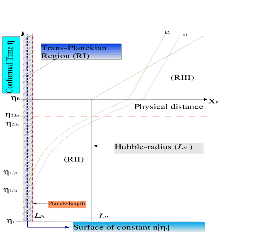
Figure 1: Sketch of the relevant regions for our model including the Trans-Planckian region where the WKB approximation for the mode equation breaks down. The horizontal axis is physical distance, the vertical axis conformal time. The red (dotted) line indicates the Planck or string length, the distance where the usual dispersion relation becomes invalid. The green (solid) line which is vertical during the period of inflation which lasts from $\eta_{i}$ to $\eta_{R}$, is the boundary between Regions II and III, the regions where the mode evolution is oscillatory or frozen, respectively. The two thin lines for which the distance grows exponentially during the period of inflation indicate the physical wavelengths of two fixed comoving modes $k_{1}$ and $k_{2}$. As is evident, they start out in Region I, the Trans-Planckian region, at early times, and then cross Region II to end up in Region III during the later stages of inflation.

• Region I: when the physical wavelength of a given mode, $\lambda(\eta)\equiv(2\pi/n)a(\eta)$ is smaller than the cutoff length where the dispersion relation begins to deviate from its usual linear form. Here, it is taken to be the string length $l_{s}$: $\lambda<l_{S}$.

• Region II: when the wavelength is longer than $l_{s}$ but smaller than the Hubble radius: $l_{S}<\lambda<l_{H}$

• Region III: when the wavelength exceeds $l_{H}$, the mode has frozen out and is being squeezed as a consequence of the negative square mass term in the equation of motion: (i.e crosses the Hubble radius): $l_{H}<\lambda$.

A special feature of our dispersion relation is that, in Region I (RI), the non-linearity of the dispersion relation leads to a violation of the adiabaticity (WKB) condition. This can be quantified in the following manner. We need to compare the rate of change of the physical frequency $\omega_{phys}$, namely $\frac{d}{d\eta}(\ln w_{phys})$, with the Hubble expansion rate $\hbox{{$\cal H$}}\equiv a^{\prime}/a$. If the former is larger than the latter, then adiabaticity is violated. Thus, one defines an adiabaticity coefficient Jerome3 by:

$$\alpha(n,\eta)\,\equiv\,\left|\frac{\hbox{{$\cal H$}}}{\frac{1}{w_{phys}}\frac{dw_{phys}}{d\eta}}\right|\,.$$ (13)

If $\alpha\ll 1$ then the adiabaticity condition is violated. The solution to the modified mode equation has no time to adjust itself such that an initial lowest energy state always tracks the instantaneous lowest energy state of the time-dependent Hamiltonian of the mode. Thus, even if the initial mode wave function minimizes the energy density, it is possible that it is in an excited state when it enters the second region (RII). In this case, the initial conditions for the evolution of the mode in Regions II and III will be different than what is assumed in the usual linear theory of gravitational waves. Since short wavelength modes spend more time in the region of non-adiabatic evolution than longer wavelength ones, one could expect a change in the slope of the power spectrum of cosmological fluctuations, as initially argued in Jerome1 .

For both power law inflation when

$$a(\eta)\,=\,\frac{l_{0}}{|\eta|^{1+\alpha}}$$ (14)

with some constant $\alpha\geq 0$, and for exponential inflation when

$$a(\eta)\,=\,\frac{l_{0}}{|\eta|}$$ (15)

we see that

$$\hbox{{$\cal H$}}\,\equiv\,\frac{a^{\prime}}{a}\,=\,(1+\alpha)\frac{1}{|\eta|}\,.$$ (16)

From Eqs. (5) and (7), and neglecting the mass term for now, it follows immediately that

$$\left|\frac{w_{phys}^{\prime}}{w_{phys}}\right|\,=\,\hbox{{$\cal H$}}kl_{s}\,.$$ (17)

Thus, the adiabaticity coefficient is

$$\alpha(n,\eta)\,\simeq\,\frac{\lambda}{l_{S}}\,,$$ (18)

where $\lambda$ is the physical wavelength corresponding to $k$. It follows that the adiabaticity condition is violated in Region I and we should hence expect modifications to the power spectrum.

II.2 Minimum Energy Density Initial Conditions

In Ref.Jerome1 , following Ref.Brown78 , it was argued that since the WKB approximation is not valid in the Trans-Planckian regime, we cannot choose as our initial conditions the Bunch-Davies vacuum. Instead we have to choose the state which initially minimizes the energy density of the field. With this prescription, the initial value of the mode function becomes Jerome1

$$\mu(\eta=\eta_{i})\,=\,\frac{1}{\sqrt{2\omega(\eta_{i})}}=\frac{1}{\sqrt{2n_{eff}}}\,,$$ (19)

and from the minimal energy density requirement we obtain:

$$\mu^{\prime}(\eta=\eta_{i})\,=\,\pm i\sqrt{\frac{n_{eff}}{2}}\,.$$ (20)

Here, $\eta_{i}$ is the initial time at which we choose to minimize the energy density.

Other relevant mode-dependent times are:

• $\eta_{1}$, the time when the mode labeled by a fixed comoving wavenumber $n$ crosses from Region I to Region II, is given by

  $$|\eta_{1}|^{1+\alpha}\,=\,{{l_{0}}\over{l_{s}}}{{2\pi}\over n}\,\equiv\,\frac{2\pi}{n\epsilon}\,,$$ (21)

  thus defining a constant $\epsilon\ll 1$.

• $\eta_{2}$, the time when the mode crosses the Hubble radius, i.e. exits from Region II into Region III, is given by

  $$|\eta_{2}|\,=\,\frac{2\pi}{n}(1+\alpha)$$ (22)

III Spectrum in the Case of Minimal Energy Initial Conditions

In this section, we present approximate analytical solutions for the mode functions obtained using the modified dispersion relation derived above, and compute the resulting power spectrum. For each mode, we solve the mode equation in each of the three regions (see Figure 1) and apply the standard matching conditions at the boundaries between the regions.

III.1 Region I (RI)

Inserting the dispersion relation (12) into the mode equation (11) and making use of (5) and of the form of the scale factor for an exponentially expanding background (15) - for simplicity we will focus on this case, i.e. on $\alpha=0$ - we obtain

$$\mu^{\prime\prime}(\eta)+\left[\frac{\exp(2n\epsilon|\eta|)}{\epsilon^{2}|\eta|^{2}}-\frac{a^{\prime\prime}}{a}\right]\mu(\eta)\,=\,0\,.$$ (23)

In Region I, the argument in the exponential in (23) is large, i.e. $2n\epsilon|\eta|>1$, and hence we can approximate the equation of motion in the following way: we can drop the second term - the squeezing term - in the square parentheses of (23) since it is suppressed compared to the first term. In the first term, we replace $\eta$ by $\eta_{1}$ in the denominator since the time dependence in the exponential overwhelms the time dependence of the other factors. Thus, the approximate form of the equation of motion Eq.(24) in Region I becomes:

$$\mu^{\prime\prime}(\eta)\,+\,\frac{e^{2n\epsilon|\eta|}n^{2}}{4\pi^{2}}\mu(\eta)\,=\,0\,.$$ (24)

After the change of variables

$$x\,\equiv\,\frac{\exp(n\epsilon|\eta|)}{2\pi\epsilon}\,,$$ (25)

the equation (24) takes the form

$$x^{2}\mu^{\prime\prime}\,+\,x\mu^{\prime}\,+\,x^{2}\mu\,=\,0\,,$$ (26)

which is nothing but Bessel’s differential equation of zeroth order. The solution can be written as

$$\mu(x)\,=\,AJ_{0}(x)\,+\,BY_{0}(x)\,,$$ (27)

where $J_{0}$ and $Y_{0}$ denote the Bessel functions and $A$ and $B$ are constants.

Since we are interested in the high energy behavior of this solution (recall that we are in the Trans-Planckian regime), we need the asymptotic representations for large arguments of the zeroth-order Bessel functions.

$$J_{0}(x)\,\sim\,\sqrt{\frac{2}{\pi x}}\left[\cos(x-\frac{\pi}{4})\right]\,, \forall\ x\gg 1$$ (28)

$$Y_{0}(x)\,\sim\,\sqrt{\frac{2}{\pi x}}\left[\sin(x-\frac{\pi}{4})\right]\,, \mbox{$\forall\ x\gg 1$}\,.$$ (29)

Recalling the expression for $x$, the asymptotic solution $\mu=\mu_{I}$ in (RI) reads

$$\mu_{I}(\eta)=2\sqrt{\epsilon}\ e^{-n\epsilon|\eta|/2}\left[A_{1}\cos\left(\frac{e^{n\epsilon|\eta|}}{2\pi\epsilon}-\pi/4\right)+A_{2}\sin\left(\frac{e^{n\epsilon|\eta|}}{2\pi\epsilon}-\pi/4\right)\right]$$ (30)

Note that in terms of the variable $x$, the two distinguished mode-dependent times $\eta_{1}$ and $\eta_{2}$ take the form

$$x_{1}\, = \,\frac{e^{n\epsilon|\eta_{1}|}}{2\pi\epsilon}=\frac{e^{2\pi}}{2\pi\epsilon}\gg 1$$ (31)

$$x_{2}\, = \,\frac{e^{n\epsilon|\eta_{2}|}}{2\pi\epsilon}=\frac{e^{2\pi\epsilon}}{2\pi\epsilon}$$ (32)

In terms of $x$, the solution reads

$$\mu_{I}(x)\,=\,\sqrt{\frac{2}{\pi x}}\left(A_{1}\cos(x-\pi/4)+A_{2}\sin(x-\pi/4)\right)$$ (33)

The coefficients $A_{1}$ and $A_{2}$ are determined by the initial conditions. We choose minimal energy density initial conditions. To implement these, we compute the derivative of $\mu$ and use

$$\frac{d}{d\eta}\mu(\eta)\,=\,\frac{dx}{d\eta}\frac{d}{dx}\mu(x)=n\epsilon x\frac{d}{dx}\mu(x)$$ (34)

From Eqs. (28) and (29)

$$J_{0}^{\prime}(x)\,\simeq\,-n\epsilon\sqrt{\frac{2x}{\pi}}\left[\sin(x-\pi/4)+\frac{1}{2x}\cos(x-\pi/4)\right]$$ (35)

and

$$Y_{0}^{\prime}(x)\,\simeq\,n\epsilon\sqrt{\frac{2x}{\pi}}\left[\cos(x-\pi/4)-\frac{1}{2x}\sin(x-\pi/4)\right]$$ (36)

and the asymptotic form of $\mu_{I}^{\prime}$ becomes

$$\mu_{I}^{\prime}(x)\,\simeq\,n\epsilon\sqrt{\frac{2x}{\pi}}\left[-A_{1}\sin(x-\pi/4)+A_{2}\cos(x-\pi/4)\right]$$ (37)

To solve for $A_{1}$ and $A_{2}$ we need to apply the minimum energy density conditions Eqs. (19) and (20), but cast in terms of $x_{i}$ instead of $|\eta_{i}|$.

$$A_{1}\cos(x_{i}-\pi/4)+A_{2}\sin(x_{i}-\pi/4)\, = \,\sqrt{\frac{\pi x_{i}}{4n_{eff_{i}}}}$$ (38)

$$-A_{1}\sin(x_{i}-\pi/4)+A_{2}\cos(x_{i}-\pi/4)\, = \,\pm\frac{i}{n\epsilon}\sqrt{\frac{\pi n_{eff_{i}}}{4x_{i}}}$$ (39)

We can now use the fact that $\epsilon\ll 1$ and the condition that $n\epsilon|\eta|\gg 1$ to guide us through our approximations. Solving for $A_{1}$ and $A_{2}$ we get

$$A_{1}\, = \,\sqrt{\frac{\pi x_{i}}{4n_{eff_{i}}}}\cos(x_{i}-\pi/4)\mp\frac{i}{n\epsilon}\sqrt{\frac{\pi n_{eff_{i}}}{4x_{i}}}\sin(x_{i}-\pi/4)$$ (40)

$$A_{2}\, = \,\sqrt{\frac{\pi x_{i}}{4n_{eff_{i}}}}\sin(x_{i}-\pi/4)\pm\frac{i}{n\epsilon}\sqrt{\frac{\pi n_{eff_{i}}}{4x_{i}}}\cos(x_{i}-\pi/4)$$ (41)

Comparing the two terms in each expression, we find that

$$A_{1}\, \simeq \,\sqrt{\frac{\pi x_{i}}{4n_{eff_{i}}}}\cos(x_{i}-\pi/4)$$ (42)

$$A_{2}\, \simeq \,\sqrt{\frac{\pi x_{i}}{4n_{eff_{i}}}}\sin(x_{i}-\pi/4)$$ (43)

Eq. (33) thus gives us the following solution in Region I

$$\mu_{I}(x)\,=\,\frac{1}{\sqrt{2n_{eff_{i}}}}\sqrt{\frac{x_{i}}{x}}\left[\cos(x_{i}-\pi/4)\cos(x-\pi/4)+\sin(x_{i}-\pi/4)\sin(x-\pi/4)\right]$$ (44)

or, more compactly,

$$\mu_{I}(x)\,=\,\frac{1}{\sqrt{2n_{eff_{i}}}}\sqrt{\frac{x_{i}}{x}}\cos(x_{i}-x)$$ (45)

III.2 Region II (RII)

In Region II, the adiabaticity condition is not violated, and thus the mode functions $\mu=\mu_{II}$ are oscillatory, i.e.

$$\mu_{II}(\eta)\,=\,B_{1}e^{in\eta}+B_{2}e^{-in\eta}$$ (46)

or equivalently in terms of $x$

$$\mu_{II}(x)\,=\,B_{1}(2\pi\epsilon)^{i/\epsilon}x^{i/\epsilon}+B_{2}(2\pi\epsilon)^{-i/\epsilon}x^{-i/\epsilon}$$ (47)

$$\mu_{II}^{\prime}(x)\,=\,in\left[B_{1}(2\pi\epsilon)^{i/\epsilon}x^{i/\epsilon}-B_{2}(2\pi\epsilon)^{-i/\epsilon}x^{-i/\epsilon}\right]\,.$$ (48)

The coefficients $B_{1}$ and $B_{2}$ are determined by the matching conditions at the time $|\eta_{1}|=\frac{2\pi}{n\epsilon}$

$$\mu_{I}(|\eta_{1}|)=\mu_{II}(|\eta_{1}|)$$

$$\mu^{\prime}_{I}(|\eta_{1}|)=\mu^{\prime}_{II}(|\eta_{1}|)$$ (49)

or their equivalent in terms of the variable $x$. Recall that, in terms of the $x$ variable, $\mu_{I}(x_{1})$ and $\mu_{I}^{\prime}(x_{1})$ are given by

$$\mu_{I}(x_{1})\, = \,\sqrt{\frac{\ln|2\pi\epsilon x_{i}|}{4\pi n\epsilon}}x^{-1/2}\cos(x_{1}-x_{i})$$ (50)

$$\mu_{I}^{\prime}(x)\, \simeq \,\sqrt{\frac{n\epsilon\ln|2\pi\epsilon x_{i}|}{4\pi}}\sin(x_{i}-x_{1})\,,$$ (51)

where we have again used the fact that $\epsilon\ll 1$ and $n\epsilon|\eta|\gg 1$. To abbreviate the notation, we introduce the variable

$$\hbox{{$\cal A$}}_{i}\,\equiv\,\sqrt{\ln|2\pi\epsilon x_{i}|}\,.$$ (52)

Then, the matching conditions (III.2) (making use of the explicit value of $x_{1}$ from Eq.(31)) read

$$\frac{e^{-\pi}}{\sqrt{2n}}\hbox{{$\cal A$}}_{i}\cos(x_{i}-x_{1})\,=\,B_{1}(2\pi\epsilon)^{i/\epsilon}x_{1}^{i/\epsilon}+B_{2}(2\pi\epsilon)^{-i/\epsilon}x_{1}^{-i/\epsilon}$$ (53)

$$\frac{-ie^{\pi}}{\sqrt{2n}}\frac{\hbox{{$\cal A$}}_{i}}{2\pi}\sin(x_{i}-x_{1})\,=\,B_{1}(2\pi\epsilon)^{i/\epsilon}x^{i/\epsilon}-B_{2}(2\pi\epsilon)^{-i/\epsilon}x^{-i/\epsilon}$$ (54)

The coefficients $B_{1}$ and $B_{2}$ are thus given by

$$B_{1}\,=\,\frac{\hbox{{$\cal A$}}_{i}}{2\sqrt{2n}}((2\pi\epsilon)^{-i/\epsilon}x_{1}^{-i/\epsilon}\left[e^{-\pi}\cos(x_{i}-x_{1})-i\frac{e^{\pi}}{2\pi}\sin(x_{i}-x_{1})\right]$$ (55)

$$B_{2}\,=\,\frac{\hbox{{$\cal A$}}_{i}}{2\sqrt{2n}}((2\pi\epsilon)^{i/\epsilon}x_{1}^{i/\epsilon}\left[e^{-\pi}\cos(x_{i}-x_{1})+i\frac{e^{\pi}}{2\pi}\sin(x_{i}-x_{1})\right]\,.$$ (56)

This time, we must keep all the terms in the coefficients since they are all of the same order. Thus, the solution of the mode function in (RII), Eq.(47), reads

$$\mu_{II}(x)\,=\,\frac{\hbox{{$\cal A$}}_{i}}{2\sqrt{2n}}\left[\left(\frac{x}{x_{1}}\right)^{i/\epsilon}\left(e^{-\pi}\cos(x_{i}-x_{1})-i\frac{e^{\pi}}{2\pi}\sin(x_{i}-x_{1})\right)+\left(\frac{x}{x_{1}}\right)^{-i/\epsilon}\left(e^{-\pi}\cos(x_{i}-x_{1})+i\frac{e^{\pi}}{2\pi}\sin(x_{i}-x_{1})\right)\right]$$

or, more compactly,

$$\mu_{II}(x)\,=\,\frac{\hbox{{$\cal A$}}_{i}}{\sqrt{2n}}\left[e^{-\pi}\cos(x_{i}-x_{1})\cos\left(\frac{\ln|x/x_{1}|}{\epsilon}\right)+\frac{e^{\pi}}{2\pi}\sin(x_{i}-x_{1})\sin\left(\frac{\ln|x/x_{1}|}{\epsilon}\right)\right]$$ (57)

III.3 The Power Spectrum

Now we are in a position to compute the power spectrum. Assuming ${\cal O}(1)$ coupling between the growing mode in Region III and $\mu_{II}$, the non-decaying mode mode in Region III is

$$\mu_{III}(\eta)\,\simeq\,Ca(\eta)$$ (58)

where the constant $C$ is fixed by matching $\mu_{III}$ with $\mu_{II}$ at the Hubble-crossing time $|\eta_{2}|$ (see Eq.(22))

$$\mu_{III}(|\eta_{2}|)\,=\,Ca(|\eta_{2}|)\,=\,C\frac{l_{0}}{|\eta_{2}|}$$ (59)

In terms of the variable $x$ the matching conditions are

$$\mu_{III}(x_{2})\,=\,Cn\frac{l_{0}}{2\pi}\,=\,\mu_{II}(x_{2})\,,$$ (60)

and hence

$$C\,=\,\frac{2\pi}{nl_{0}}\mu_{II}(x_{2})\,.$$ (61)

The power spectrum $P_{\phi}$ for our scalar field $\phi$ is defined as

$$P_{\phi}(n)\,=\,n^{3}|\phi(k)|^{2}\,=\,n^{3}a^{-2}|\mu(n)|^{2}\,.$$ (62)

The spectral index $n_{T}$ for gravitational waves is defined by

$$P_{\phi}(n)\,=\,A_{\rm T}n^{n_{\rm T}}\,,$$ (63)

where $A_{\rm T}$ is the amplitude of the spectrum.

Combining (62) and (58) we obtain

$$P_{\phi}(n)\,=\,n^{3}\left|\frac{\mu}{a}\right|^{2}\,=\,n^{3}|C|^{2}\,.$$ (64)

Making use of (61) and (57) we get

$$P_{\phi}(n)\, = \,\frac{(2\pi)^{2}n}{l_{0}^{2}}\left|\mu_{II}(|\eta_{2}|)\right|^{2}$$ (65)

$$= \,\frac{2\pi^{2}}{l_{0}^{2}}|\hbox{{$\cal A$}}_{i}|^{2}\hbox{{$\cal J$}}(|\eta_{i}|,|\eta_{1}|,|\eta_{2}|)|^{2}$$ (66)

where $\hbox{{$\cal J$}}(|\eta_{i}|,|\eta_{1}|,|\eta_{2}|)$ will yield oscillations in the spectrum of a particular form, and is given by

$$\hbox{{$\cal J$}}(|\eta_{i}|,|\eta_{1}|,|\eta_{2}|)\,=\,e^{-\pi}\cos\left(\frac{e^{n\epsilon|\eta_{i}|}-e^{n\epsilon|\eta_{1}|}}{2\pi\epsilon}\right)\cos\left(\frac{n\epsilon|\eta_{2}|}{n\epsilon|\eta_{1}|}\right)+\frac{e^{\pi}}{2\pi}\sin\left(\frac{e^{n\epsilon|\eta_{i}|}-e^{n\epsilon|\eta_{1}|}}{2\pi\epsilon}\right)\sin\left(\frac{n\epsilon|\eta_{2}|}{n\epsilon|\eta_{1}|}\right)$$ (67)

Plugging in the values for $|\eta_{1}|$ and $|\eta_{2}|$ and making more transparent the $n\epsilon|\eta_{i}|$-dependence of $\hbox{{$\cal J$}}(n,\epsilon,|\eta_{i}|)$, we obtain

$$\hbox{{$\cal J$}}(n,\epsilon,|\eta_{i}|)\,=\,\cos\left(\frac{e^{n\epsilon|\eta_{i}|}}{2\pi\epsilon}\right)\left[e^{-\pi}\cos\left(\frac{2\pi}{\epsilon}\right)\cos\left(\frac{e^{2\pi}}{2\pi\epsilon}\right)-\frac{e^{\pi}}{2\pi}\sin\left(\frac{e^{2\pi}}{2\pi\epsilon}\right)\right]$$

$$+\sin\left(\frac{e^{n\epsilon|\eta_{i}|}}{2\pi\epsilon}\right)\left[e^{-\pi}\cos\left(\frac{2\pi}{\epsilon}\right)\sin\left(\frac{e^{2\pi}}{2\pi\epsilon}\right)-\frac{e^{\pi}}{2\pi}\cos\left(\frac{e^{2\pi}}{2\pi\epsilon}\right)\right]$$ (68)

The amplitude and spectral index of the power spectrum can be read off by inserting the expression (52) for $\hbox{{$\cal A$}}_{i}$ and making use of the definition (25) of the variable $x$, yielding

$$A_{\rm T}n^{n_{\rm T}}\,=\,\frac{2\pi^{2}}{l_{0}^{2}}\ n\epsilon|\eta_{i}|\ |\hbox{{$\cal J$}}(n,\epsilon,|\eta_{i}|)|^{2}\,.$$ (69)

III.4 Discussion

From our main result (69) we draw the following conclusions. Given our modified dispersion relation for fluctuations, the spectrum of gravitational waves in an exponentially expanding background is characterized by a non-vanishing spectral tilt of $n_{\rm T}=1$. In addition, there are oscillations in the spectrum with a characteristic dependence on $n$. This result was obtained working to leading order in $\epsilon$.

The fact that the spectrum is not scale-invariant but blue-shifted is due to the fact that the shorter wavelengths are subject to the modified dispersion relation for a longer time, leading to a higher excitation level of the modes when their wavelength is equal to the cutoff scale after which the dispersion relation becomes linear. This is similar to what happens in models with a discrete space-time, or in analog models from condensed matter physics where the modes feel the granular nature of matter on scales of the order of the atomic separation resulting in a departure from the linear dispersion relation.

We would like to point to an important observation regarding Eq.(69). We made it explicit to show how the combination $n\epsilon|\eta_{i}|$ appears both in the oscillatory function $\cal J$ and in Eq.(69). We see that to get a scale invariant spectrum without oscillations, it suffices to modify the prescription for the initial conditions and postulate that the modes are created at a mode-dependent initial time $|\eta_{i}|$ for which $n|\eta_{i}|\equiv$constant (this is similar to what is postulated to occur in the analyses of minmal; Ho ). We will discuss later on a better derivation of what the initial conformal time might be by linking the fact that having T-duality at the basis of our dispersion relation, i.e. as our Trans-Planckian physics, is similar as modifying our space-time metric by adding to it a minimal length which is of the order of the string length $l_{S}$. This could be linked to non-commutative space-time or to a stringy space-time uncertainty relation which was studied earlier in Ref.Ho . We will return to that point at the end of our article since it is of a more speculative nature.

IV Spectrum in the Case of an Instantaneous Minkowski Vacuum

To test the dependence of our previous result on the initial conditions we adopt another choice of initial conditions, the instantaneous Minkowski vacuum as an alternative to Eqs.(19) and (20). That is, at $|\eta|=|\eta_{i}|$ the mode function now satisfy:

$$\mu(|\eta_{i}|)=\frac{1}{\sqrt{2n}}$$ (70)

$$\mu^{\prime}(|\eta_{i}|)=\pm\sqrt{\frac{n}{2}}$$ (71)

IV.1 The Trans-Planckian Region (RI)

Following the same steps as in the case of the minimum energy density initial state, we set the initial conditions at a fixed time $\eta_{i}$ in the Trans-Planckian region (RI). We start with the general solution in Region I from Eqs.(33) and (37) and match them to the initial values (70) in order to determine the new coefficients $A_{1}$ and $A_{2}$. The result is

$$A_{1}\,\simeq\,\sqrt{\frac{\pi x_{i}}{4n}}\cos(x_{i}-\pi/4)$$ (72)

$$A_{2}\,\simeq\,\sqrt{\frac{\pi x_{i}}{4n}}\sin(x_{i}-\pi/4)\,,$$ (73)

and the mode function $\mu_{I}(x)$ is thus given by

$$\mu_{I}(x)\,=\,\frac{1}{\sqrt{2n}}\sqrt{\frac{x_{i}}{x}}\cos(x_{i}-x)\,.$$ (74)

IV.2 Region II

In Region II where the WKB approximation is valid, we have plane wave solutions for the mode functions as in Eqs. (47) and (48). The mode functions are matched at the time $|\eta_{1}|$ when the physical wavelength of a mode equals the minimal length $l_{S}$, that is

$$\mu_{I}(x_{1})\,=\,\mu_{II}(x_{1})$$ (75)

$$\mu_{I}^{\prime}(x_{1})\,=\,\mu_{II}^{\prime}(x_{1})$$ (76)

These yield two equations for the coefficients $B_{1}$ and $B_{2}$ which can be solved to get

$$B_{1}\,\simeq\,\frac{-i}{2}\sqrt{\frac{x_{i}x_{1}}{2n}}\frac{\sin(x_{i}-x_{1})}{(2\pi\epsilon x_{1})^{i/\epsilon}}$$ (77)

$$B_{2}\,\simeq\,\frac{i}{2}\sqrt{\frac{x_{i}x_{1}}{2n}}\sin(x_{i}-x_{1})(2\pi\epsilon x_{1})^{i/\epsilon}$$ (78)

The mode solution $\mu_{II}(x)$ in Region II is thus given by:

$$\mu_{II}(x)\,=\,\sqrt{\frac{x_{i}x_{1}}{2n}}\sin(x_{i}-x_{1})\sin\left[\frac{\ln|x/x_{1}|}{\epsilon}\right]\,.$$ (79)

IV.3 The Power Spectrum Revisited

Again assuming that the growing mode in Region III picks up ${\cal O}(1)$ of the amplitude of $\mu_{II}$ at the matching time $x_{2}$, the solution $\mu_{III}$ in Region III is given by

$$\mu_{III}\,=\,Ca(\eta)\,,$$ (80)

with the constant $C$ determined by $C=\frac{2\pi}{l_{0}n}\mu_{II}(x_{2})$ or, expanded out

$$C\,=\,\frac{2\pi}{l_{0}n}\sqrt{\frac{x_{i}x_{1}}{2n}}\sin(x_{i}-x_{1})\sin\left[\frac{\ln|x_{2}/x_{1}|}{\epsilon}\right]$$ (81)

The power spectrum $P_{\phi}(n)$ thus becomes

$$P_{\phi}(n)\, = \,A_{S}n^{n_{T}}\,=\,n^{3}|C|^{2}$$ (82)

$$= \,\frac{2\pi^{2}}{l_{0}^{2}}x_{i}x_{1}\sin^{2}(x_{i}-x1)\sin^{2}\left[\frac{\ln|x_{2}/x_{1}|}{\epsilon}\right]$$ (83)

In terms of conformal time,

$$P_{\phi}(n)\,=\,\frac{e^{2\pi}e^{n\epsilon|\eta_{i}|}}{2l_{S}^{2}}\sin^{2}\left[\frac{e^{n\epsilon|\eta_{i}|}-e^{2\pi}}{2\pi\epsilon}\right]\cos^{2}\left(\frac{2\pi}{\epsilon}\right)$$ (84)

IV.4 Discussion

The striking difference between our previous result obtained using the minimum energy density calculations and that found here using the instantaneous Minkowski vacuum initial conditions is the dependence of the power spectrum on the comoving wave number $n$. We see from Eq. (84) that the dependence on $n$ is exponential while from Eq. (69) the dependence on $n$ is linear. Thus, for the instantaneous Minkowski vacuum we get an exponentially blue spectrum (note that the quantity $n\epsilon|\eta_{i}|$ which appears in the exponential is much greater than one).

If, instead of imposing initial conditions for all modes at a fixed time, we use the alternative discussed section III.4, namely assume a minimal length in our theory and argue that initial conditions should be set on a surface of constant $n|\eta_{i}|$ which would correspond to the surface on which the physical mode are created, and setting

$$n|\eta_{i}|\,=\,\frac{\ln|2\pi^{2}\epsilon\delta|}{\epsilon}\,,$$ (85)

(for some fixed number $\delta$) we would obtain the following spectrum:

$$A_{\rm S}n^{n_{\rm S}-1}\,=\,\frac{e^{2\pi}\pi^{2}\delta}{l_{S}^{2}}\sin^{2}\left(\pi\delta-\frac{e^{2\pi}}{2\pi\epsilon}\right)\cos^{2}\left(\frac{2\pi}{\epsilon}\right)$$ (86)

which is scale invariant spectrum without any oscillations which depend on the comoving wavenumber $n$. Thus, for this initial time prescription we arrive at the same conclusion as in the case of minimal energy initial conditions. This is not a real surprise since in this case all modes spend the same amount of time in the trans-Planckian region.

V Conclusions

In this paper we have studied the spectrum of gravitational waves which results when the usual linear dispersion relation for the wave equation is replaced by the non-linear dispersion relation which results when assuming that the wave propagator is consistent with the T-duality symmetry of string theory. This modified dispersion relation differs from the linear one on length scales smaller than the string scale.

We have shown that the modified dispersion relation leads to a non-adiabatic evolution of the mode functions in the trans-Planckian region. If, as is usual in an inflationary cosmology, the initial conditions for fluctuations are set for all modes at the same initial time, this modification, in turn, leads to a change in the slope of the spectrum of gravitational waves. Instead of a scale-invariant spectrum, a spectrum with blue tilt given by a spectral index $n_{T}=1$ results. In addition, the spectrum has characteristic oscillations.

Our results are based on studying the evolution of a test scalar field on our expanding inflationary background. According to the theory of cosmological perturbations, each gravitational wave polarization mode obeys the same equation as such a test scalar field. The scalar metric fluctuations, in turn, obey an equation with a slightly different squeezing factor MFB ; RHBrev2 . The difference in the equations of motion, however, is in general only important on scales larger than the Hubble radius, and even then only if the equation of state of the background is changing in time. Thus, it is reasonable to expect that a similar analysis to the one given in this paper applies to scalar metric fluctuations. The result for scalar metric fluctuations would then be a spectrum with blue tilt $n_{S}=2$, inconsistent with recent data WMAP . If the only change to the equation of motion for cosmological fluctuations in the context of string theory on trans-Planckian scales were the change in the dispersion relation discussed in this paper, our results would imply a deep problem in realizing successful inflation in the context of string theory. However, as discussed in Ho , there are other aspects of string theory, e.g. the space-time uncertainty relation, which must be considered, and these considerations could well restore the prediction of a scale-invariant spectrum in the case when the background space in exponentially expanding.

In conclusion, we hope to have convinced the reader that, assuming that there was a period of cosmological inflation, the basic principles of string theory are clearly testable in cosmological observations. Final predictions, however, will have to await a better understanding of the equations of string theory on trans-Planckian scales.