Quantum fluctuations on a thick de Sitter brane

Abstract

We investigate quantum fluctuations on a de Sitter (dS) brane, which has its own thickness, in order to examine whether or not the finite thickness of the brane can act as a natural cut-off for the Kaluza-Klein (KK) spectrum. We calculate the amplitude of the KK modes and the bound state by using the zeta function method after a dimensional reduction. We show that the KK amplitude is finite for a given brane thickness and in the thin wall limit the standard surface divergent behavior is recovered. The strength of the divergence in the thin wall limit depends on the number of dimensions, e.g., logarithmic on a two dimensional brane and quadratic on a four dimensional brane. We also find that the amplitude of the bound state mode and KK modes depends on the choice of renormalization scale; and for fixed renormalization scales the bound state mode is insensitive to the brane thickness both for two and four-dimensional dS branes.

I Introduction

Recent progress in string theory suggests that our universe is not four-dimensional, in reality, but is a four-dimensional submanifold, called a “brane” embedded into a higher dimensional spacetime, called the “bulk”. The model which was proposed by Randall and Sundrum (RS) succeeds in the localization of gravity around the brane due to a fascinating process, i.e., through the warping of the extra-dimension Randall:1999vf . This model has been given phenomenological grounds from various aspects of higher-dimensional theories of gravity, e.g., in terms of cosmology, higher-dimensional black holes and the AdS/CFT correspondence (see e.g., Maartens:2003tw ; Brax:2004xh for reviews).

In spite of much effort by various authors, there seem to be few theoretical predictions of such a braneworld with cosmological observations. In the RS type brane model, information from a higher-dimensional gravity theory is carried by Kaluza-Klein (KK) modes, which are massive modes from the observers’ point of view, who are living on the brane. Thus, if KK modes are detected in future observations this may uniquely determine whether or not our universe is a brane.

The quantum fluctuations that are usually assumed to be produced during the inflationary phase are considered as natural seeds for the perturbations, which form the various cosmological structures and produce the CMB anisotropy we see today. Thus, in the braneworld scenario, the quantum fluctuations may imprint information from the KK modes on today’s cosmological observations.

In some braneworld models, the inflaton whose dynamics induces inflation on the brane is naturally set into the bulk as a result of a dimensional reduction of some higher-dimensional gravitational theory, e.g., dilaton or moduli fields, as discussed in Kobayashi:2000yh ; Himemoto:2000nd ; Koyama:2003yz . In various bulk inflaton models, quantum fluctuations have been well examined Kobayashi:2000yh ; Koyama:2003yz ; Sago:2001gi ; Naylor:2004ua ; Pujolas:2005mu . However, it is well-known that a Casimir surface divergence remains on the brane even after UV regularization. This type of divergence prevents us from evaluating quantum fluctuations exactly on the brane, though there are approaches to deal with such a problem, e.g., see Naylor:2004ua ; Pujolas:2005mu . In all previous cases mentioned above it was assumed that the brane was infinitesimally thin, which is inherited from the original proposal by RS.

From a more realistic point of view; however, it is rather natural for the brane to have a thickness. Furthermore, string theory, which brane world is based upon, has a minimum length scale, i.e., the string length scale $l_{s}=\sqrt{\alpha^{\prime}}$, where $\alpha^{\prime}$ is the inverse of string tension. This supports the possibility that, in reality, the brane has a finite thickness, rather than being infinitesimally thin. Various thick brane models have been discussed, see e.g., DeWolfe:1999cp ; Gremm:1999pj ; Csaki:2000fc ; Arefeva:2000qv ; Giovannini:2001xg ; Kobayashi:2001jd ; Sasakura:2002tq ; Sasakura:2002hv ; Ghoroku:2003kc ; Bronnikov:2003gg . Then, we are interested in whether or not “the finite thickness of the brane, if it exists, acts as a natural cut-off for the KK spectrum.” In this article, we discuss this speculative idea by investigating the behavior of the KK modes in an explicit thick de Sitter (dS) brane model.

We consider a simple thick dS brane model which is supported by a bulk scalar field $\phi$ with an axion-like potential, originally discussed by Wang Wang:2002pk ; Guerrero:2005xx . Then, we introduce another scalar field $\chi$ as a bulk inflaton Kobayashi:2000yh ; Himemoto:2000nd type field and investigate its quantum fluctuations. We use the zeta function method in conjunction with the dimensional reduction approach developed in Naylor:2004ua . We show that the brane thickness regularizes the UV behavior of the KK modes and compare its amplitude with that of the bound state mode, which is relevant from the observational point of view.

This article is organized as follows: in Sec. II, we introduce a thick dS brane model supported by a bulk scalar field. In Sec. III, bearing the bulk inflaton model in mind, we introduce another quantized scalar field and make the necessary preparations to evaluate the amplitude. We take the dimensional reduction approach and calculate the amplitude using generalized zeta functions. In Sec. IV, focusing on a two dimensional dS brane (three-dimensional bulk), we calculate the amplitude of quantum fluctuations and show that the brane thickness acts as a natural cut-off for the KK spectrum. The surface divergence in the thin wall limit is logarithmic. We also show that the bound state amplitude depends on the renormalization scale; however, for a fixed renormalization scale it is almost independent of the brane thickness. Then in Sec. V, we discuss quantum fluctuations on a four dimensional dS brane (five-dimensional bulk) and obtain results similar to that for the two-dimensional case. The leading order surface divergence in the thin wall limit is quadratic in this case. In Sec. VI, we summarize our results and mention future work related to these issues. In Appendix A, we derive the fluctuation amplitude of the bound state on two and four dimensional dS branes, respectively. In Appendix B, we demonstrate the classical stability of the thick brane model both against tensor and scalar perturbations.

II A thick de Sitter brane model

We consider the Einstein theory coupled to a bulk scalar field,

$$S=\frac{1}{2}\int d^{d+1}x\sqrt{-g}\Bigl{(}\stackrel{{\scriptstyle(d+1)}}{{R}}-\bigl{(}\partial\phi\bigr{)}^{2}-2V(\phi)\Bigr{)}\,,$$ (1)

where the potential of the scalar field is given by the axion like form Wang:2002pk ; Guerrero:2005xx ,

$$V(\phi)=V_{0}\Bigl{(}\cos\Bigl{[}\frac{\phi}{\phi_{0}}\Bigr{]}\Bigr{)}^{2(1-\sigma)}\,.$$ (2)

Note that we shall set $\kappa_{d+1}^{2}=1$ in this article.

We shall assume a static configuration, namely $\phi$ depends on only the bulk coordinate and make the following metric ansatz

$$ds^{2}=b(z)^{2}(dz^{2}+\gamma_{\mu\nu}dx^{\mu}dx^{\nu})\,,$$ (3)

where $\gamma_{\mu\nu}$ denotes the metric of $d$-dimensional de Sitter (dS) spacetime. Following the above ansatz, we obtain the Einstein equations

$$\frac{d(d-1)}{2}\Bigl{(}\frac{b^{\prime}}{b}\Bigr{)}^{2}-\frac{d(d-1)}{2}H^{2}=\frac{1}{2}\phi^{\prime 2}-b^{2}V\,,$$

$$(d-1)\Bigl{[}\frac{b^{\prime\prime}}{b}+\frac{1}{2}(d-4)\Bigl{(}\frac{b^{\prime}}{b}\Bigr{)}^{2}-\frac{1}{2}(d-2)H^{2}\Bigr{]}=-\frac{1}{2}\phi^{\prime 2}-b^{2}V$$ (4)

and the field equation for the scalar field is

$$\phi^{\prime\prime}+(d-1)\frac{b^{\prime}}{b}\phi^{\prime}-b^{2}\frac{\partial V}{\partial\phi}=0\,,$$ (5)

where the prime $\,{}^{\prime}\,$ denotes the derivative with respect to $z$. Note that only two of these three equations are independent. For this potential, we find the solutions

$$b(z)=\left(\cosh\left(\frac{Hz}{\sigma}\right)\right)^{-\sigma}\,,\qquad\phi(z)=\phi_{0}\sin^{-1}\left(\tanh\left(\frac{Hz}{\sigma}\right)\right)\,,$$ (6)

where

$$H^{2}=\frac{2\sigma V_{0}}{(d-1)[1+(d-1)\sigma]}\,,\quad\phi_{0}=\sqrt{(d-1)\sigma(1-\sigma)}~{}.$$ (7)

This solution represents a dS domain wall whose energy is localized at $z=0$, i.e., the center of the wall. The parameter $\sigma$ has the meaning of the thickness of the wall (brane) from the physical point of view. In order to keep the positivity in the square root, we should restrict the range to Wang:2002pk

$$0<\sigma<1~{}.$$ (8)

III Quantized scalar field perturbations

Our purpose is to discuss the quantized scalar field perturbations on a thick, inflating brane model. We achieve this by introducing another scalar field $\chi$, which is coupled to the domain wall configuration and its fluctuations. Hence, we add the action of the scalar field $\chi$ to the original action Eq. (1), i.e.,

$$S=\frac{1}{2}\int d^{d+1}x\sqrt{-g}\Bigl{(}\stackrel{{\scriptstyle(d+1)}}{{R}}-\bigl{(}\partial\phi\bigr{)}^{2}-2V(\phi)\Bigr{)}+\frac{1}{2}\int d^{d+1}x\sqrt{-g}\Bigl{(}-\bigl{(}\partial\chi\bigr{)}^{2}-\xi\stackrel{{\scriptstyle(d+1)}}{{R}}\chi^{2}\Bigr{)}\,,$$ (9)

where $\xi$ is the scalar curvature coupling.

As discussed in Olum:2002ra ; Graham:2002yr the coupling of the field $\chi$ to $\phi$ can be ignored because its backreaction to the domain wall geometry is only important at higher order, $O(\chi^{2})$. This assumption allows us to treat the $\chi$-field contribution perturbatively. The minimally coupled case, $\xi=0$, will be of particular interest, because the perturbation equations are very similar to those for tensor perturbations of the metric (see Appendix B).

III.1 Dimensional reduction approach

We shall evaluate the amplitude of the quantum field $\chi$ based on a dimensional reduction of the higher dimensional canonically quantized field. This method has been already discussed in Naylor:2004ua and we refer the reader to this reference for more details.

In this method, the action of $\chi$ is rewritten as

$$S_{\chi}=\frac{1}{2}\int d^{d+1}x\sqrt{-g}\,\chi\Bigl{(}\Box_{d+1}-\xi\stackrel{{\scriptstyle(d+1)}}{{R}}\Bigr{)}\chi\,,$$ (10)

where we set a regulator boundary at $z=L$ in order to obtain a well-posed quantum field theory on the dimensionally reduced spacetime. Then, the bulk modes become discrete and the solution is written as

$$\chi(z,x^{\mu})=\sum_{n}F_{n}(z)\varphi_{n}(x^{\mu})H^{1/2}\,,$$ (11)

where $\varphi_{n}$ has the dimension of a scalar field in the $d$-dimensional dS spacetime. Due to the maximal symmetry of dS spacetime, we can integrate out the dependence on the transverse directions, $x^{\mu}$, assuming that the vacuum respects the dS invariance. Hence, we shall drop it in the amplitude.

Integrating the action with respect to $z$, it is reduced to the summation of theories of a $d$-dimensional massive scalar field with mass $m_{n}$:

$$S_{\chi}=\frac{1}{2}\sum_{n}\int d^{d}x\sqrt{-\gamma}\,\varphi_{n}(x^{\mu})\Bigl{(}\Box_{d}-m_{n}^{2}\Bigr{)}\varphi_{n}(x^{\mu})\,,$$ (12)

where we employed the normalization condition

$$2\int^{L}_{0}(H\,dz)\,b^{d-1}(z)F_{q_{n}}(z)F_{q_{n}^{\prime}}(z)=\delta_{nn^{\prime}}\,.$$ (13)

Note that the multiplying factor of two is due to the ${\mathbb{Z}}_{2}$-symmetry. The mass-squared $m_{n}^{2}$ is given by

$$m_{n}^{2}=q_{n}^{2}H^{2}+\frac{(d-1)^{2}}{4}H^{2}\,.$$ (14)

We introduce a new function $f_{q_{n}}(z):=b^{(d-1)/2}(z)F_{q_{n}}(z)$, which obeys the Schrödinger like equation

$$-f_{q_{n}}^{\prime\prime}(z)+\tilde{V}(z)H^{2}f_{q_{n}}=q_{n}^{2}H^{2}f_{q_{n}}(z)\,,$$ (15)

where

$$\tilde{V}(z):=-\bigl{(}\xi_{c}-\xi\bigr{)}\Bigl{\{}d(d-1)+\frac{2d}{\sigma}\Bigr{\}}\frac{1}{\cosh^{2}(Hz/\sigma)}\,.$$ (16)

For the minimally coupled case, $\xi=0$, this potential reduces to the one for the tensor metric perturbations (i.e., gravitons), Eq. (104). The reason that we choose a massless scalar field as a probe in this article is to obtain some insight into the graviton case (and also for technical simplicity). In Fig. 1, we plot the potential for the $d=4$ case explicitly for $\xi=0$. It is evident that the potential becomes deeper for smaller values of $\sigma$.

Figure 1: The potential for a minimally coupled bulk scalar field perturbation is shown as a function of $Hz$ for a four-dimensional dS wall. The thick, thick-dashed and dashed curves correspond to the cases of $\sigma=0.01,0.05,0.1$, respectively.

Figure 2: $\nu/\sigma$ is plotted as a function of thickness, $\sigma$. The thick, thick-dashed and dashed curves correspond to the cases for $\xi=0,3/32,3/20$, respectively.

The solution of the KK modes is

$$f_{q_{n}}(z)=C_{1}P^{i\sigma q_{n}}_{\nu}(x)+C_{2}P^{-i\sigma q_{n}}_{\nu}(x)\,,$$ (17)

where $P^{\mu}_{\nu}(x)$ denotes the Legendre functions of the first kind, $x:=\tanh(Hz/\sigma)$ and

$$\nu:=\frac{\sqrt{1+4(\xi_{c}-\xi)(d(d-1)\sigma^{2}+2d\sigma)}-1}{2}\,.$$ (18)

The coupling

$$\xi_{c}=\frac{d-1}{4d}$$ (19)

denotes the conformal coupling strength, e.g., for the $d=2$ case $\xi_{c}=1/8$ and for the $d=4$ case $\xi_{c}=3/16$. In this article, we restrict the coupling to the range $0\leq\xi\leq\xi_{c}$.

The mass of the bound state mode is given by

$$q_{0}=\frac{i\nu}{\sigma}\,,$$ (20)

which has a maximal value of $(d-1)/2$ at $\xi=0$. For $\xi<0$, the bound state becomes tachyonic and non-normalizable. For $\xi=0$, it is the zero mode and for $\xi=\xi_{c}$ it becomes the lowest mass KK mode, irrespective of the choice of $\sigma$. In Fig. 2, we plot $\nu/\sigma$ as a function of $\sigma$ for several choice of $\xi$. We find that this ratio is almost independent of $\sigma$. Note that the $\xi=0$ case is equivalent to the bulk tensor perturbations.

III.2 The zeta function method

Given the functions $f_{q_{n}}(z)$, the vacuum expectation value is defined by

$$\langle\chi^{2}(z)\rangle=\frac{2H}{b^{d-1}(z)}\sum_{n}f_{q_{n}}^{2}(z)\langle\varphi_{q_{n}}^{2}(x)\rangle\,,$$ (21)

where the factor of two is due to the ${\mathbb{Z}}_{2}$-symmetry. From now on, we shall discuss the quantized field theory in Euclidean space, i.e., the metric is

$$ds^{2}=b^{2}(z)\bigl{(}dz^{2}+d\Omega_{d}^{2}\bigr{)}\,,$$ (22)

where $d\Omega_{d}$ is the line element of $S^{d}$ with unit radius, whose volume is given by

$$V_{S^{d}}=\frac{2\pi^{\frac{d+1}{2}}}{\Gamma(\frac{d+1}{2})}\,.$$ (23)

Thus, in order to consider the quantum fluctuations of a $d$-dimensional field, we assume that the vacuum is given by the Euclidean vacuum, which corresponds to the dS invariant, Bunch-Davis vacuum in the original Lorentzian spacetime.

For the $d$-sphere, $S^{d}$, any local quantities are related to global ones by simply dividing by the volume of the sphere (a property of maximally symmetric spaces; see Naylor:2004ua ). Thus, we are particularly interested in the local vacuum expectation value as only a function of $z$ (one non-trivial dimension), implying

$$K_{n}(t)=\int d^{d}{x}\sqrt{\gamma}K_{n}(x,x;t)\,,$$ (24)

where $K_{n}$ is the dS heat kernel for each mode $n$, see Naylor:2004ua . Thus, due to the maximal symmetry of dS space, the global heat kernel is simply related to the local one by

$$K_{n}(t)=\frac{V_{S^{d}}}{H^{d}}K_{n}(x,x;t)~{}.$$ (25)

At this stage it is convenient to rescale the amplitude as

$$\langle\tilde{\chi}^{2}(z)\rangle=\frac{b(z)^{d-1}V_{S^{d}}}{H^{d+1}}\langle\chi^{2}(z)\rangle\,,$$ (26)

where overall factors can be restored at the end of the calculation. Now we may sum up all the KK modes in Eq. (21); however, as is well known, a naive summation over all the KK modes gives rise to unwanted divergences.

To deal with such a problem, we construct the local zeta function, $\zeta(z,s)$, along the lines of reference Naylor:2004ua , where the parameter $s$ is initially assumed to be $s>(d+1)/2$ in $(d+1)$-dimensions. Once we obtain such a zeta function, after analytic continuation to $s\to 1$, we end up with

$$\langle\tilde{\chi}^{2}(z)\rangle=\lim_{s\to 1}\tilde{\zeta}(z,s)\,,$$ (27)

where

$$\tilde{\zeta}(z,s):=\frac{b(z)^{d-1}V_{S^{d}}}{H^{d+1}}\zeta(z,s)=\frac{1}{\Gamma(s)}\int^{\infty}_{0}dt\,t^{s-1}K(z,t)\,.$$ (28)

$K(z,t)$ is the local heat kernel defined as

$$K(z,t)=2\sum_{n=1}^{\infty}f_{q_{n}}^{2}(z)K_{n}(t)\,,$$ (29)

and

$$K_{n}(t)=\sum_{j=0}^{\infty}d_{j}\,e^{-[q_{n}^{2}+(j+1/2)^{2}]H^{2}t}\,,$$ (30)

where $d_{j}$ is the degeneracy for each mode $j$ given by

$$d_{j}=\left(2j+d-1\right)\frac{(j+d-2)!}{j!(d-1)!}\,,$$ (31)

is the global heat kernel for each KK mode. Note that the dimension of $\tilde{\zeta}$ is slightly different to the case discussed in Naylor:2004ua , because of a difference in dimension of the warp factor.

III.3 Contour integral representation of the local zeta function

First, as a resolution to the subtle nature of the continuous modes, we introduce another boundary at $z=L$. This then enables us to evaluate the zeta function using the residue theorem, based on certain assumptions relating to the zeros of the function in the contour. Then, after constructing such a zeta function we show that we can take the one brane limit $L\to\infty$ in a well defined manner.

The solution for the scalar field perturbations in general dimensions is given by

$$f_{q}(z)=N_{q}\Bigl{(}\alpha_{q}P^{iq\sigma}_{\nu}(x)-\beta_{q}R^{iq\sigma}_{\nu}(x)\Bigr{)}\,,$$ (32)

where for convenience, we choose the second solution $R^{iq\sigma}_{\nu}(x)$ to satisfy

$$P^{iq\sigma}_{\nu}(x)R^{iq\sigma}_{\nu}{}^{\prime}(x)-R^{iq\sigma}_{\nu}(x)P^{iq\sigma}_{\nu}{}^{\prime}(x)=\frac{1}{1-x^{2}}\,,$$ (33)

where $x=\tanh(Hz/\sigma)$. There are several candidates for $R^{iq\sigma}_{\nu}(x)$ such as

$$\frac{\Gamma(-iq\sigma+\nu+1)}{\Gamma(iq\sigma+\nu+1)}Q^{iq\sigma}_{\nu}(x)\,,\quad-\frac{\pi}{2i\sinh(\pi q\sigma)}P^{-iq\sigma}_{\nu}(x)\,,$$ (34)

and so on. For now we do not need to specify the explicit form of the second solution $R^{iq\sigma}_{\nu}(x)$, but only use the property of the Wronskian in Eq. (33).

To be specific, let us consider the case of Neumann boundary conditions. The boundary conditions at the center of the thick brane and the second boundary are respectively

$$f_{q}^{\prime}(z)|_{z=0}=0\,,\quad f_{q}^{\prime}(z)|_{z=L}=0\,.$$ (35)

Note, the thick brane is not a boundary, we just fix the $z$ derivative of the field at a point to obtain a well-posed eigenvalue equation. From these boundary conditions, we get an equation which determines the KK mass spectrum as

$$P^{iq\sigma}_{\nu}{}^{\prime}(0)R^{iq\sigma}_{\nu}{}^{\prime}(x_{L})-P^{iq\sigma}_{\nu}{}^{\prime}(x_{L})R^{iq\sigma}_{\nu}{}^{\prime}(0)=0\,.$$ (36)

We denote the solutions for the eigen-equation as $q_{n}~{}(n=1,2,3,\cdots)$ whose eigenfunctions are

$$f_{q_{n}}(z)=N_{q_{n}}\Bigl{(}\alpha_{q_{n}}P^{iq_{n}\sigma}_{\nu}(x)-\beta_{q_{n}}R^{iq_{n}\sigma}_{\nu}(x)\Bigr{)}\,,$$ (37)

where

$$\frac{\alpha_{q_{n}}}{\beta_{q_{n}}} = \frac{R^{iq_{n}\sigma}_{\nu}{}^{\prime}(0)}{P^{iq_{n}\sigma}_{\nu}{}^{\prime}(0)}=\frac{R^{iq_{n}\sigma}_{\nu}{}^{\prime}(x_{L})}{P^{iq_{n}\sigma}_{\nu}{}^{\prime}(x_{L})}\,.$$ (38)

We assume $q_{1}<q_{2}<q_{3}<\cdots$, respectively. Note that the final equality is satisfied only for $q=q_{n}$. Without loss of generality, we can choose $\alpha_{q}=R^{iq\sigma}_{\nu}{}^{\prime}(0)$ and $\beta_{q}=P^{iq\sigma}_{\nu}{}^{\prime}(0)$. We shall also require the normalization constant for $n$-th mode which is found to be

$$N^{-2}_{q_{n}} = 2\int^{L}_{0}(H\,dz)\Bigl{(}\alpha_{q_{n}}P^{iq_{n}\sigma}_{\nu}(x)-\beta_{q_{n}}R^{iq_{n}\sigma}_{\nu}(x)\Bigr{)}^{2}$$ (39)

$$= -\frac{1}{\sigma q_{n}}\frac{R^{iq_{n}\sigma}_{\nu}{}^{\prime}(0)}{R^{iq_{n}\sigma}_{\nu}{}^{\prime}(x_{L})}\partial_{q}\Bigl{(}R^{iq\sigma}_{\nu}{}^{\prime}(0)P^{iq\sigma}_{\nu}{}^{\prime}(x_{L})-P^{iq\sigma}_{\nu}{}^{\prime}(0)R^{iq\sigma}_{\nu}{}^{\prime}(x_{L})\Bigr{)}_{q=q_{n}}\,.$$

Note that in the second step we used Eq. (3.8) and integrated by parts.

Now we have all the necessary tools to calculate the zeta function by applying the residue theorem as follows: from the equations given above, the normalized mode functions can be written as

$$f_{q_{n}}^{2}(z)=\frac{\sigma q_{n}G(q_{n},z)}{\partial_{q}F(q)|_{q=q_{n}}}\,,$$ (40)

where,

$$F(q)=-\Bigl{(}R^{iq\sigma}_{\nu}{}^{\prime}(0)P^{iq\sigma}_{\nu}{}^{\prime}(x_{L})-P^{iq\sigma}_{\nu}{}^{\prime}(0)R^{iq\sigma}_{\nu}{}^{\prime}(x_{L})\Bigr{)}$$ (41)

and

$$G(q,z)=\Bigl{(}R^{iq\sigma}_{\nu}{}^{\prime}(0)P^{iq\sigma}_{\nu}(x)-P^{iq\sigma}_{\nu}{}^{\prime}(0)R^{iq\sigma}_{\nu}(x)\Bigr{)}\Bigl{(}R^{iq\sigma}_{\nu}{}^{\prime}(x_{L})P^{iq\sigma}_{\nu}(x)-P^{iq\sigma}_{\nu}{}^{\prime}(x_{L})R^{iq\sigma}_{\nu}(x)\Bigr{)}\,.$$ (42)

This form is essential in order to apply the residue theorem. Whence, the zeta function can be written as a contour integral in the complex $u$ plane

$$\tilde{\zeta}(z,s) = 2\mu^{2(s-1)}\sum_{n=1}^{\infty}\,\sum_{j=0}^{\infty}\frac{d_{j}\,f_{q_{n}}^{2}(z)}{\bigl{[}q_{n}^{2}+(j+{d-1\over 2})^{2}\bigr{]}^{s}H^{2s}}$$ (43)

$$= 2\mu^{2(s-1)}\sum_{n=1}^{\infty}\sum_{j=0}^{\infty}\frac{\sigma q_{n}G(q_{n},z)}{\partial_{q}F(q)|_{q=q_{n}}}{d_{j}\over\bigl{[}q_{n}^{2}+(j+{d-1\over 2})^{2}\bigr{]}^{s}H^{2s}}$$

$$= 2\mu^{2(s-1)}\oint_{C}\frac{du}{2\pi i}\frac{\sigma uG(u,z)}{F(u)|_{u=q_{n}}}\sum_{j=0}^{\infty}\frac{d_{j}}{[u^{2}+(j+{d-1\over 2})^{2}]^{s}H^{2s}}\,\,,$$

where the poles at $u=q_{n}$ are on the positive side of real axis and therefore, the closed contour $C$ has to be taken around the positive real axis in general. Note that we have introduced a mass scale $\mu$ to keep the dimension. This term is in fact the renormalization scale and groups with any divergent terms in the expression for the amplitude. Then, given the fact that there are no poles in the complex $u$-plane, besides those on the real axis, we can naturally deform the contour $C$ into $C^{\prime}$ (see Fig. 3)

$$\tilde{\zeta}(z,s)=2\mu^{2(s-1)}\oint_{C^{\prime}}\frac{du}{2\pi i}\frac{\sigma uG(u,z)}{F(u)|_{u=q_{n}}}\sum_{j=0}^{\infty}\frac{d_{j}}{[u^{2}+(j+{d-1\over 2})^{2}]^{s}H^{2s}}\,,$$ (44)

which is composed of a line parallel to the imaginary axis with a small real part and a large semi circle on the positive real half of the complex plane, which is depicted in Fig 3. As we mentioned previously, initially keeping $s$ larger than $(d+1)/2$, the contribution from the larger semi-circle becomes negligible.

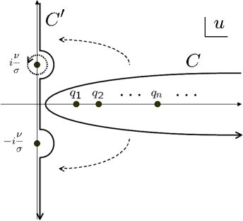
Figure 3: The contour $C$, used to evaluate the KK amplitude. The poles on the real axis $q_{i}\,(i=1,2,\cdots)$ correspond to the KK modes, while those on the imaginary axis correspond to the bound state. We can deform $C$ into $C^{\prime}$ because there are no poles in the complex plane besides those on the real and imaginary axes. The closed contour depicted by the dotted line is used to evaluate the bound state amplitude.

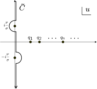
Figure 4: The contour $\tilde{C}$, used to evaluate the total amplitude.

A similar approach has been used e.g., in Saharian:2004ih for infinitely thin Minkowski branes in a bulk AdS space; however, in our case the contour we have to construct is complicated by the presence of the poles which come from the bound state; and as we shall see, it will be convenient to evaluate the bound state contribution separately. Therefore, as it turns out, we shall only focus on the total amplitude from now on.

In particular, we are primarily interested in calculating the mode functions on the brane at $z=0\,(x=0)$, i.e.,

$$\left.\frac{G(u,z)}{F(u)}\right|_{z=0} = \frac{\bigl{(}R^{iu\sigma}_{\nu}{}^{\prime}(0)P^{iu\sigma}_{\nu}(0)-P^{iu\sigma}_{\nu}{}^{\prime}(0)R^{iu\sigma}_{\nu}(0)\bigr{)}\bigl{(}R^{iu\sigma}_{\nu}{}^{\prime}(x_{L})P^{iu\sigma}_{\nu}(0)-P^{iu\sigma}_{\nu}{}^{\prime}(x_{L})R^{iu\sigma}_{\nu}(0)\bigr{)}}{-\bigl{(}R^{iu\sigma}_{\nu}{}^{\prime}(0)P^{iu\sigma}_{\nu}{}^{\prime}(x_{L})-P^{iu\sigma}_{\nu}{}^{\prime}(0)R^{iu\sigma}_{\nu}{}^{\prime}(x_{L})\bigr{)}}$$ (45)

$$= \frac{P^{iu\sigma}_{\nu}{}^{\prime}(x_{L})R^{iu\sigma}_{\nu}(0)-R^{iu\sigma}_{\nu}(x_{L}){}^{\prime}P^{iu\sigma}_{\nu}(0)}{\bigl{(}R^{iu\sigma}_{\nu}{}^{\prime}(0)P^{iu\sigma}_{\nu}{}^{\prime}(x_{L})-P^{iu\sigma}_{\nu}{}^{\prime}(0)R^{iu\sigma}_{\nu}{}^{\prime}(x_{L})\bigr{)}}$$

$$= \frac{P^{iu\sigma}_{\nu}{}^{\prime}(x_{L})P^{-iu\sigma}_{\nu}(0)-P^{-iu\sigma}_{\nu}{}^{\prime}(x_{L})P^{iu\sigma}_{\nu}(0)}{\bigl{(}P^{-iu\sigma}_{\nu}{}^{\prime}(0)P^{iu\sigma}_{\nu}{}^{\prime}(x_{L})-P^{iu\sigma}_{\nu}{}^{\prime}(0)P^{-iu\sigma}_{\nu}{}^{\prime}(x_{L})\bigr{)}}\,,$$

where in the first step we used the Wronskian relation Eq. (33) and in the final step we specified the second mode function as

$$R^{iq\sigma}_{\nu}(x)=-\frac{\pi}{2i\sinh(\pi q\sigma)}P^{-iq\sigma}_{\nu}(x)\,.$$ (46)

Two types of decomposition are possible:

$$\frac{P^{iu\sigma}_{\nu}{}^{\prime}(x_{L})P^{-iu\sigma}_{\nu}(0)-P^{-iu\sigma}_{\nu}{}^{\prime}(x_{L})P^{iu\sigma}_{\nu}(0)}{P^{-iu\sigma}_{\nu}{}^{\prime}(0)P^{iu\sigma}_{\nu}{}^{\prime}(x_{L})-P^{iu\sigma}_{\nu}{}^{\prime}(0)P^{-iu\sigma}_{\nu}{}^{\prime}(x_{L})}$$ (47)

$$= \frac{P^{iu\sigma}_{\nu}(0)}{P^{iu\sigma}_{\nu}{}^{\prime}(0)}-\frac{P^{iu\sigma}_{\nu}{}^{\prime}(x_{L})}{P^{iu\sigma}_{\nu}{}^{\prime}(0)}\frac{2i\sinh(\pi u\sigma)}{\pi}\frac{1}{P^{iu\sigma}_{\nu}{}^{\prime}(0)P^{-iu\sigma}_{\nu}{}^{\prime}(x_{L})-P^{iu\sigma}_{\nu}{}^{\prime}(x_{L})P^{-iu\sigma}_{\nu}{}^{\prime}(0)}$$

$$= \frac{P^{-iu\sigma}_{\nu}(0)}{P^{-iu\sigma}_{\nu}{}^{\prime}(0)}+\frac{P^{-iu\sigma}_{\nu}{}^{\prime}(x_{L})}{P^{-iu\sigma}_{\nu}{}^{\prime}(0)}\frac{2i\sinh(\pi u\sigma)}{\pi}\frac{1}{P^{-iu\sigma}_{\nu}{}^{\prime}(0)P^{iu\sigma}_{\nu}{}^{\prime}(x_{L})-P^{-iu\sigma}_{\nu}{}^{\prime}(x_{L})P^{iu\sigma}_{\nu}{}^{\prime}(0)}\,.$$

It is important to note that the second term on the second line is negligible in the $x_{L}\to 1$ limit on the upper half of the complex $u$-plane, while the second term on the third line is negligible in the same limit on the lower-half of complex $u$-plane. Thus, in the single brane limit we use the first term on the second and third lines as the single brane propagator on the upper and lower half of the complex plane, respectively.

In the single brane propagator given above, $P^{iu\sigma}_{\nu}(0)/P^{iu\sigma}_{\nu}{}^{\prime}(0)$ has poles that are situated on the negative imaginary axis, corresponding to purely decaying modes, plus the bound state contribution at $u=i\nu/\sigma$. However, as we mentioned above, $P^{iu\sigma}_{\nu}(0)/P^{iu\sigma}_{\nu}{}^{\prime}(0)$ is used for the upper half of the complex plane and we need not worry about the purely decaying modes. Thus, we only need to deal with the bound state mode at $u=i\nu/\sigma$ in the calculation of the KK amplitude. Similarly, the exact opposite occurs for $P^{-iu\sigma}_{\nu}(0)/P^{-iu\sigma}_{\nu}{}^{\prime}(0)$ and we only need to deal with the pole at $u=-i\nu/\sigma$.

The remaining problem then concerns the avoidance of the bound state poles at $u=\pm i{\nu}/{\sigma}$. We avoid the bound state poles by deforming the contour to $C^{\prime}$, as depicted in Fig. 3, when we evaluate the KK amplitude. However, this contour gives a non-zero contribution (from the bound state poles) when taking the Cauchy principal value on the imaginary axis. This contribution simply corresponds to the subtraction of the bound state from the total amplitude; we can calculate the bound state amplitude separately, see Appendix A. Thus, it will be rather convenient for us to shift the contour over the upper pole to $\tilde{C}$, as depicted in Fig. 4. This is equivalent to adding the bound state contribution with a counter-clockwise contour (the closed dotted line in Fig. 3) to $C^{\prime}$. Then, by integrating along the contour $\tilde{C}$ and subtracting the bound state contribution, we can obtain the desired KK amplitude. This is the approach we shall take to evaluate the KK amplitude in this article.

IV Kaluza-Klein Amplitude: $d=2$ Case

To demonstrate the method discussed in the previous section as simply as possible, we first evaluate the amplitude of the quantum fluctuations on the brane for $d=2$. That is, we construct the zeta function for the case of the two-sphere in the transverse dimensions with one non-trivial bulk dimension.

IV.1 Amplitude of the KK modes

The zeta function for total amplitude at the center of the wall is

$$\tilde{\zeta}(0,s) = 4\mu^{2(s-1)}\oint_{\tilde{C}}\frac{du}{2\pi i}\frac{\sigma uG(u,0)}{F(u)}\sum_{j=0}^{\infty}\frac{(j+1/2)}{[u^{2}+(j+1/2)^{2}]^{s}H^{2s}}$$ (48)

$$= \frac{4\mu^{2(s-1)}}{\pi H^{2s}}\sin[\pi(s-1)]\,\,{\rm P}\int_{0}^{2\nu/\sigma}dUU\frac{\sigma G(e^{\pi i/2}U,0)}{F(e^{\pi i/2}U)}\sum_{j=0}^{\infty}\frac{(j+1/2)}{\bigl{[}U^{2}-(j+1/2)^{2}\bigr{]}^{s}}\,,$$

where $U=e^{-\pi i/2}u$ and we use the property

$$\frac{G(e^{\pi i/2}U,0)}{F(e^{\pi i/2}U)}=\frac{G(e^{-\pi i/2}U,0)}{F(e^{-\pi i/2}U)}=\frac{P^{-U\sigma}_{\nu}(0)}{2P^{-U\sigma}_{\nu}{}^{\prime}(0)}\,.$$ (49)

Here, Roman “${\rm P}$” (not to be confused with the Legendre function of the first kind) means taking the Cauchy principal value in order to deal with the pole at $U=\nu/\sigma$. In Fig. 4, the contribution from the anti-clockwise semi-circle around $u=i\nu/\sigma$ cancels with that from the clockwise semi-circle around $u=-i\nu/\sigma$.

In the following, we shall divide the integral into two; i.e., for $U>2\nu/\sigma$ which we denote as the “UV piece” and that for $0<U<2\nu/\sigma$ which we denote as the “IR piece.” We emphasize that the reason for this splitting is solely for technical reasons and that the choice of division has no physical significance. We can set the split at any value of $O(1)$.

To begin with, for the UV piece we will use the following asymptotic expansion formula, e.g., see Ref. Elizalde:1996zk , for large $U$, i.e.,

$$\sum_{j=0}^{\infty}\frac{(j+1/2)}{\bigl{[}U^{2}-(j+1/2)^{2}\bigr{]}^{s}}=-\frac{1}{2}U^{-2s+2}\Bigl{[}\frac{1}{s-1}-\frac{1}{\Gamma(s)}\sum_{j=1}^{\infty}\frac{\Gamma(j+s-1)}{j!}U^{-2j}\partial_{a}{\zeta}_{H}(-2j,a)\Big{|}_{a=1/2}\Bigr{]}\,.$$ (50)

Then, for the IR piece we employ the standard binomial expansions:

$$\sum_{j=0}^{\infty}\frac{j+1/2}{\bigl{[}(j+1/2)^{2}-U^{2}\bigr{]}^{s}}=\sum_{J=0}^{\infty}\frac{\Gamma(s+J)}{J!\Gamma(s)}U^{2J}\zeta_{H}(2s+2J-1,\frac{1}{2})\,,$$ (51)

which is valid for the range $0<U<1/2$; while for the range $1/2<U<2\nu/\sigma<1$ we must use Elizalde:1996zk ; CREP

$$\sum_{j=0}^{\infty}\frac{j+1/2}{\bigl{[}(j+1/2)^{2}-U^{2}\bigr{]}^{s}}=\frac{1}{2}\left(\frac{1}{(\frac{1}{4}-U^{2})^{s}}+\sum_{J=0}^{\infty}\frac{\Gamma(s+J)}{J!\Gamma(s)}U^{2J}\left(2\zeta_{H}(2s+2J-1,\frac{1}{2})-\left(\frac{1}{2}\right)^{-2s-2J}\right)\right)\,.$$ (52)

Then, the total amplitude on the center at the wall is given by the summation of both pieces

$$\tilde{\zeta}(0,s) = \tilde{\zeta}_{\rm UV}(0,s)+\tilde{\zeta}_{\rm IR}(0,s)\,.$$ (53)

First, let us consider the analytic continuation of the UV piece

$$\tilde{\zeta}_{\rm UV}(0,s) = -\frac{2\mu^{2(s-1)}\sin[\pi(s-1)]}{\pi H^{2s}}$$

$$\times \int^{\infty}_{2\nu/\sigma}dU\frac{\sigma G(e^{\pi i/2}U,0)}{F(e^{\pi i/2}U)}U^{-2s+3}\left[\frac{1}{s-1}-\frac{1}{\Gamma(s)}\sum_{j=1}^{\infty}\frac{\Gamma(j+s-1)}{j!}U^{-2j}\partial_{a}\zeta_{H}(-2j,a)\Big{|}_{a=1/2}\right]\,.$$

Given the following relation ab

$$\frac{P^{-U\sigma}_{\nu}(0)}{P^{-U\sigma}_{\nu}{}^{\prime}(0)}=-{1\over 2}\frac{\Gamma(-\frac{\nu}{2}+\frac{U\sigma}{2})\Gamma(\frac{\nu}{2}+\frac{U\sigma}{2}+\frac{1}{2})}{\Gamma(\frac{\nu}{2}+\frac{U\sigma}{2}+1)\Gamma(-\frac{\nu}{2}+\frac{U\sigma}{2}+\frac{1}{2})}\,$$ (55)

and by employing the asymptotic expansion for large $U$ of the Gamma functions ab we find the following asymptotic series, which in $d$-dimensions is

$$\frac{P^{-U\sigma}_{\nu}(0)}{P^{-U\sigma}_{\nu}{}^{\prime}(0)}=\sum_{\ell=0}^{\infty}w_{\ell}(\sigma,\xi)U^{-1-2\ell}\,,$$ (56)

where $\nu$ is given by Eq. (18) and

$$w_{0}(\sigma,\xi) = -\frac{1}{\sigma}\,,$$

$$w_{1}(\sigma,\xi) = \frac{(2+\sigma(d-1))(1+d(-1+4\xi))}{8\sigma^{2}}=\frac{1}{2\sigma}\tilde{V}(0)\,,$$ (57)

$$w_{2}(\sigma,\xi) = -\frac{(2+\sigma(d-1))(1+d(-1+4\xi))\left(8+6\sigma\left(1+d\left(-1+4\xi\right)\right)+3\sigma^{2}\left(-1+d\right)\left(1+d\left(-1+4\xi\right)\right)\right)}{128\sigma^{4}}\,.$$

The subtraction of the $w_{0}$ term just corresponds to that of the trivial background, whereas the $w_{1}$ term corresponds to the tadpole graph, see Olum:2002ra ; Graham:2002yr . Here, we require only the term $w_{0}$, in order to regularize the $d=2$ case. For the $d=4$ case, terms up to $w_{1}$ are required.

Thus, after analytic continuation to $s\to 1$, we obtain the UV amplitude

$$H^{2}\lim_{s\to 1}\tilde{\zeta}_{\rm UV}(0,s) = -2\Bigl{\{}\int^{\infty}_{2\nu/\sigma}dUU\,\sigma\Bigl{[}\frac{P^{-U\sigma}_{\nu}(0)}{P^{-U\sigma}_{\nu}{}^{\prime}(0)}-\frac{w_{0}(\sigma,\xi)}{U}\Bigr{]}-w_{0}(\sigma,\xi)\left(\frac{2\nu}{\sigma}\right)\Bigr{\}}\,.$$ (58)

As for the IR piece it is already finite in the limit $s\to 1$; however, because of the poles on the imaginary axis we make the principle value prescription, i.e.,

$$\tilde{\zeta}_{\rm IR}(0,s) = \frac{4\mu^{2(s-1)}}{\pi H^{2s}(-1)^{s}}\sin[\pi(s-1)]\,{\rm P}\int^{1/2}_{0}dU\frac{\sigma UG(e^{\pi i/2}U,0)}{F(e^{\pi i/2}U)}\sum_{J=0}^{\infty}\frac{\Gamma(s+J)}{J!\Gamma(s)}U^{2J}\zeta_{H}(2s+2J-1,\frac{1}{2})$$ (59)

$$+ \frac{2\mu^{2(s-1)}}{\pi H^{2s}(-1)^{s}}\sin[\pi(s-1)]\,{\rm P}\int^{2\nu/\sigma}_{1/2}dU\frac{\sigma G(e^{\pi i/2}U,0)}{F(e^{\pi i/2}U)}$$

$$\times \left(\frac{1}{(\frac{1}{4}-U^{2})^{s}}+\sum_{J=0}^{\infty}\frac{\Gamma(s+J)}{J!\Gamma(s)}U^{2J}\left(2\zeta_{H}(2s+2J-1,\frac{1}{2})-\left(\frac{1}{2}\right)^{-2s-2J}\right)\right)\,,$$

where if $2\nu/\sigma<1/2$ the second term is to be dropped. Then, given the Laurent expansion of the Hurwitz zeta function

$$\zeta_{H}(2s-1,\frac{1}{2})=\frac{1}{2(s-1)}-\psi(1/2)+O(s-1)\,,$$ (60)

we find that there is only a contribution from $J=0$ in both terms. Thus, in the limit $s\rightarrow 1$, we obtain

$$H^{2}\lim_{s\to 1}\tilde{\zeta}_{\rm IR}(0,s) = -{\rm P}\int^{2\nu/\sigma}_{0}dU\frac{2\sigma G(e^{\pi i/2}U,0)}{F(e^{\pi i/2}U)}U$$

$$= 2\int^{2\nu/\sigma}_{0}\frac{dU}{U-\nu/\sigma}\left(U\frac{\Gamma(-\nu/2+U\sigma/2+1)\Gamma(\nu/2+U\sigma/2+1/2)}{\Gamma(\nu/2+U\sigma/2+1)\Gamma(-\nu/2+U\sigma/2+1/2)}-\frac{1}{\sqrt{\pi}}\frac{\nu}{\sigma}\frac{\Gamma(\nu+1/2)}{\Gamma(\nu+1)}\right)\,,$$

where in the final step, we used the fact that

$${\rm P}\int_{0}^{2x_{0}}dx\frac{f(x)}{x-x_{0}} = {\rm P}\int_{0}^{2x_{0}}dx\frac{f(x)}{x-x_{0}}-{\rm P}\int_{0}^{2x_{0}}dx\frac{f(x_{0})}{x-x_{0}}$$ (62)

$$= \int^{2x_{0}}_{0}dx\frac{f(x)}{x-x_{0}}-\int^{2x_{0}}_{0}dx\frac{f(x_{0})}{x-x_{0}}\,,$$

where $f(x)$ is an arbitrary regular function. The second term, which is equal to zero, eliminates the singularity at $x=x_{0}$ in the first term. This technique will also be used for the $d=4$ case.

Finally, we obtain the regularized total amplitude

$$\langle\tilde{\chi}^{2}(0)\rangle_{\rm tot} = \lim_{s\to 1}\left(\tilde{\zeta}_{\rm UV}(0,s)+\tilde{\zeta}_{\rm IR}(0,s)\right)\,.$$ (63)

As discussed in the preceding section the KK amplitude is obtained by subtracting the bound state amplitude, which is evaluated in Appendix A,

$$\langle\tilde{\chi}^{2}(0)\rangle_{\rm KK}=\langle\tilde{\chi}^{2}(0)\rangle_{\rm tot}-\langle\tilde{\chi}^{2}(0)\rangle_{\rm bs}\,.$$ (64)

Interestingly, the total amplitude $\langle\tilde{\chi}^{2}(0)\rangle_{\rm tot}$ does not depend on the renormalization scale $\mu$, whereas as shown in Appendix $A$ the bound state contribution $\langle\tilde{\chi}^{2}(0)\rangle_{\rm bs}$ does depend on it. Thus, the KK amplitude $\langle\tilde{\chi}^{2}(0)\rangle_{\rm KK}$ will also depend on $\mu$ as can be readily seen from Eq. (64). In other words, the dependence on $\mu$ in the bound state and KK contribution cancels when they are summed up.

IV.2 Results of numerical calculations

The total amplitude $\langle\chi^{2}(0)\rangle_{\rm tot}$ is shown in Fig. 5. For small thicknesses, the UV piece dominates the total amplitude. The leading order divergent behavior can be estimated as follows: by changing variables from $U$ to $x=U\sigma$, the UV piece can be written as

$$H^{2}\lim_{s\to 1}\tilde{\zeta}_{\rm UV}(0,s)=-2\left(\frac{1}{\sigma}\int^{\infty}_{2\nu}dx\,x\left(\frac{P^{-x}_{\nu}(0)}{P^{-x}_{\nu}{}^{\prime}(0)}+\frac{1}{x}\right)+\frac{2\nu}{\sigma}\right)\,.$$ (65)

As shown previously (see Fig. 2), $\nu/\sigma$ is almost independent of $\sigma$ and $\nu=O(\sigma)$ for $\sigma\ll 1$. Then by Taylor expanding the Gamma functions in Eq. (55) about $\nu$ we find that

$$\frac{P^{-x}_{\nu}(0)}{P^{-x}_{\nu}{}^{\prime}(0)}=-\frac{1}{x}+\frac{\nu}{2x}\left(\psi(\frac{x}{2})-2\psi(\frac{x+1}{2})+\psi(\frac{x}{2}+1)\right)+O(\sigma^{2})\,.$$ (66)

Therefore,

$$H^{2}\lim_{s\to 1}\tilde{\zeta}_{\rm UV}(0,s)=-\frac{\nu}{\sigma}\int^{\infty}_{2\nu}dx\left(\psi(\frac{x}{2})-2\psi(\frac{x+1}{2})+\psi(\frac{x}{2}+1)\right)+O(\sigma^{0}).$$ (67)

In the case of $d=2$ the divergence arises only from the leading order. Furthermore, for $x\gg 1$ the integrand behaves as $x^{-2}$ and thus, the contribution from the upper bound vanishes. However, in the opposite limit, $x\ll 1$,

$$\psi(\frac{x}{2})-2\psi(\frac{x+1}{2})+\psi(\frac{x}{2}+1)=-\frac{2}{x}+\left(-2\gamma-2\psi(1/2)\right)+O(x)\,,$$ (68)

where $\gamma=0.57721\cdots$ is Euler’s constant, and therefore

$$H^{2}\lim_{s\to 1}\tilde{\zeta}_{\rm UV}(0,s)=-\frac{2\nu}{\sigma}\ln\left(2\nu\right)+O(\sigma^{0}).$$ (69)

Thus, we find a positive logarithmic divergence in the thin wall limit.

The amplitude of the bound state is derived separately in Appendix A. Here, we recapitulate the final result,

$$H^{2}\langle\tilde{\chi}^{2}(0)\rangle_{\rm bs} = \frac{1}{\sigma}\Bigl{(}2\ln\left(\frac{\mu}{H}\right)-2\psi(1/2)-\delta_{\xi\,,0}\left(\frac{1}{2}\right)^{-2}+\sum_{J=1}^{\infty}\Big{[}2\left(\frac{\nu}{\sigma}\right)^{2J}\zeta_{H}(2J+1,\frac{1}{2})-\delta_{\xi\,,0}\left(\frac{1}{2}\right)^{-2}\Big{]}\Bigr{)}$$ (70)

$$\times \left(\int^{\infty}_{0}dy\cosh^{-2\nu}(y)\right)^{-1}\,.$$

In Fig. 6, the amplitude of the bound state is plotted as a function of the brane thickness for each coupling, with $\mu=H$. Interestingly, the resulting amplitude is almost independent of the brane thickness $\sigma$ and still finite in the thin wall limit.

Thus, as expected, the divergence of the total amplitude in the thin wall limit arises solely from the KK contribution. Regardless, for finite values of $\sigma\sim 0.1$ the total amplitude settles down to finite positive values. The result shows that the surface divergence for the KK modes can be regularized by introducing a finite brane thickness. This is one of the main results of this article.

Figure 5: The total amplitude is shown as a function of the brane thickness, $\sigma$, in the case of $d=2$. The thick, thick-dashed and dashed curves correspond to the cases of $\xi=0,1/32,1/16$, respectively.

Figure 6: The amplitude of the bound state is shown as a function of the brane thickness, $\sigma$, in the case of $d=2$, with $\mu=H$. The thick, thick-dashed and dashed curves correspond to the cases of $\xi=0,1/32,1/16$, respectively.

Figure 7: The running of the bound state is shown as a function of the renormalization scale $\ln\,\mu$ in the case of $d=2$, with $\sigma=0.01$. The vertical and horizontal axes show the bound state amplitude and $\log_{10}(\mu/H)$, respectively. The thick, thick-dashed and dashed curves correspond to the cases of $\xi=0,1/32,1/16$, respectively.

Figure 8: The relative amplitude of the KK modes to the bound state mode is shown as a function of the brane thickness, $\sigma$, for minimal coupling, $\xi=0$, for $d=2$, with $\mu=H$.

The bound state amplitude depends on the choice of renormalization scale, $\mu$. In Fig. 7, the running of the scale is shown as a function of $\mu$. It is essentially proportional to $\ln\,\mu$. The tilt becomes steeper for smaller coupling parameter $\xi$. There are several possible choices for the renormalization scale, for example, one could choose the expansion rate of the brane $\mu=H$ or another choice is the brane thickness $\mu=H/\sigma$. We still have no signature from braneworld today and therefore no quantity that we can renormalize into. The renormalization scale $\mu$ should be determined by future observations and/or experiments. In this article we just plot the running of the scale and take the optimal choice $\mu=H$ for cases where one has to make a choice. Note that from Eq. (64) the KK amplitude is also proportional to $\ln(\mu)$ with negative tilts.

It is also interesting to compare the relative amplitude of the KK modes to the bound state mode. The relative amplitude is given by

$$r:=\frac{\langle\chi^{2}(0)\rangle_{\rm KK}}{\langle\chi^{2}(0)\rangle_{\rm bs}}\ =\frac{\langle\tilde{\chi}^{2}(0)\rangle_{\rm KK}}{\langle\tilde{\chi}^{2}(0)\rangle_{\rm bs}}=\frac{\langle\tilde{\chi}^{2}(0)\rangle_{\rm tot}}{\langle\tilde{\chi}^{2}(0)\rangle_{\rm bs}}-1\,,$$ (71)

where in the final step we used Eq. (64). The result depends on the choice of the renormalization scale $\mu$ and brane thickness, $\sigma$. It is meaningful to show the plot for physically reasonable cases. As an example, in Fig. 8, we have plotted $r$ as a function of $\sigma$ for the minimally coupled case, $\xi=0$, i.e., for tensor perturbations, with $\mu=H$.

V Kaluza-Klein Amplitude: $d=4$ case

In this section, we perform the calculation for the more realistic case of $d=4$. The calculation follows in an identical manner to the $d=2$ case, if only for more tedium.

V.1 Amplitude of the KK modes

In this case the degeneracy factor for the four-sphere ($d=4$) is

$$d_{j}=\frac{1}{3}\left(j+\frac{3}{2}\right)\left(j+1\right)\left(j+2\right)\,$$ (72)

and hence, the zeta function for the total amplitude can be reduced to

$$\tilde{\zeta}(0,s) = \frac{2}{3}\mu^{2(s-1)}\oint_{\tilde{C}}\frac{du}{2\pi i}\frac{\sigma uG(u,0)}{F(u)}\sum_{j=0}^{\infty}\frac{(j+3/2)(j+1)(j+2)}{[u^{2}+(j+1/2)^{2}]^{s}H^{2s}}$$ (73)

$$= \frac{2\mu^{2(s-1)}}{3\pi H^{2s}}\sin[\pi(s-1)]\,{\rm P}\int^{\infty}_{0}dU\frac{\sigma UG(e^{\pi i/2}U,0)}{F(e^{\pi i/2}U)}\sum_{j=0}^{\infty}\frac{(j+1)(j+2)(j+\frac{3}{2})}{\bigl{[}U^{2}-(j+\frac{3}{2})^{2}\bigr{]}^{s}}\,,$$

where we used the properties of bulk propagator Eq. (49). Again, Roman “${\rm P}$” represents taking the Cauchy principal value to deal with the pole at $U=\nu/\sigma$. As for the $d=2$ case, we divide the total zeta function into a UV piece, i.e., for $U>2\nu/\sigma$; and an IR piece, i.e., for $0<U<2\nu/\sigma$. Similarly, the choice of the division is just for later convenience.

To begin with, for the UV piece we shall use the asymptotic formula Elizalde:1996zk

$$\frac{2}{3}\sum_{j=0}^{\infty}\frac{(j+3/2)(j+1)(j+2)}{\bigl{[}U^{2}-(j+3/2)^{2}\bigr{]}^{s}} = \frac{2}{3}\sum_{j=0}^{\infty}\frac{(j+3/2)^{3}}{\bigl{[}U^{2}-(j+3/2)^{2}\bigr{]}^{s}}-\frac{1}{6}\sum_{j=0}^{\infty}\frac{(j+3/2)}{\bigl{[}U^{2}-(j+3/2)^{2}\bigr{]}^{s}}\,$$ (74)

$$= (-1)^{s}\Bigg{(}-\frac{1}{12(s-1)(s-2)(s-3)}\partial_{a}^{3}\theta(-U^{2},a,s-2)+\frac{1}{12(s-1)}\partial_{a}\theta(-U^{2},a,s)$$

$$- \frac{1}{2(s-1)(s-2)}\partial_{a}\theta(-U^{2},a,s-1)\Bigg{)}_{a=3/2}\,$$

$$= -\frac{1}{12\Gamma(s)}\Bigl{[}U^{-2(s-1)}\sum_{j=0}^{\infty}\frac{\Gamma(j+s-1)}{j!}U^{-2j}\partial_{a}\zeta_{H}(-2j,a)\Big{|}_{a=3/2}$$

$$- U^{-2(s-3)}\sum_{j=0}^{\infty}\frac{\Gamma(j+s-3)}{j!}U^{-2j}\partial_{a}^{3}\zeta_{H}(-2j,a)\Big{|}_{a=3/2}$$

$$+ 6U^{-2(s-2)}\sum_{j=0}^{\infty}\frac{\Gamma(j+s-2)}{j!}U^{-2j}\partial_{a}\zeta_{H}(-2j,a)\Big{|}_{a=3/2}\Bigr{]}\,,$$

where

$$\theta(q^{2},a,s):=\sum_{j=0}^{\infty}\frac{1}{\bigl{[}(j+a)^{2}+q^{2}\bigr{]}^{s-1}}\,.$$ (75)

Then, for the IR piece, we use the following binomial expansions Elizalde:1996zk ; CREP :

$$\frac{1}{3}\sum_{j=0}^{\infty}\frac{(j+1)(j+2)(j+3/2)}{\bigl{[}(j+3/2)^{2}-U^{2}\bigr{]}^{s}}=\frac{1}{3}\sum_{J=0}^{\infty}\frac{\Gamma(s+J)}{J!\Gamma(s)}U^{2J}\left(\zeta_{H}(2s+2J-3,\frac{3}{2})-\frac{1}{4}\zeta_{H}(2s+2J-1,\frac{3}{2})\right)\,,$$ (76)

which is valid for the range $0<U<3/2$; while for the range $3/2<U<5/2$ we must use

$$\frac{1}{3}\sum_{j=0}^{\infty}\frac{(j+1)(j+2)(j+3/2)}{\bigl{[}(j+3/2)^{2}-U^{2}\bigr{]}^{s}}=\frac{1}{\left(\frac{9}{4}-U^{2}\right)^{s}}$$

$$\qquad+\sum_{J=0}^{\infty}\frac{\Gamma(s+J)}{J!\Gamma(s)}U^{2J}\left[\frac{1}{3}\left(\zeta_{H}(2s+2J-3,\frac{3}{2})-\frac{1}{4}\zeta_{H}(2s+2J-1,\frac{3}{2})\right)-\left(\frac{3}{2}\right)^{-2s-2J}\right]\,,$$

and finally, for the range $5/2<U<\frac{2\nu}{\sigma}$ we have

$$\frac{1}{3}\sum_{j=0}^{\infty}\frac{(j+1)(j+2)(j+3/2)}{\bigl{[}(j+3/2)^{2}-U^{2}\bigr{]}^{s}}=\frac{1}{\left(\frac{9}{4}-U^{2}\right)^{s}}+\frac{5}{\left(\frac{25}{4}-U^{2}\right)^{s}}$$

$$\quad+\sum_{J=0}^{\infty}\frac{\Gamma(s+J)}{J!\Gamma(s)}U^{2J}\Bigg{[}\frac{1}{3}\left(\zeta_{H}(2s+2J-3,\frac{3}{2})-\frac{1}{4}\zeta_{H}(2s+2J-1,\frac{3}{2})\right)-\left(\frac{3}{2}\right)^{-2s-2J}-5\left(\frac{5}{2}\right)^{-2s-2J}\Bigg{]}\,.$$ (78)

The total zeta function is obtained from Eq. (53).

First, let us focus on the analytic continuation of the UV piece. Some simple manipulations lead to the following expression

$$\tilde{\zeta}_{\rm UV}(0,s) = \frac{1}{12}\frac{\mu^{2(s-1)}}{H^{2s}}\int_{2\nu/\sigma}^{\infty}dU\frac{\sigma G(e^{\pi i/2}U,0)}{F(e^{\pi i/2}U)}$$ (79)

$$\times \Bigl{\{}U^{-2s+3}\sin[\pi(s-2)]\Bigl{[}\frac{1}{s-1}\partial_{a}\zeta_{H}(0,a)\Big{|}_{a=3/2}+\sum_{j=1}^{\infty}\frac{\Gamma(j+s-1)}{j!\Gamma(s)}U^{-2j}\partial_{a}\zeta_{H}(-2j,a)\Big{|}_{a=3/2}\Bigr{]}$$

$$- U^{-2s+7}\sin[\pi(s-4)]\Bigl{[}\frac{1}{(s-1)(s-2)(s-3)}\partial_{a}^{3}\zeta_{H}(0,a)\Big{|}_{a=3/2}+\frac{U^{-2}}{(s-1)(s-2)}\partial_{a}^{3}\zeta_{H}(-2,a)\Big{|}_{a=3/2}$$

$$+\frac{U^{-4}}{2(s-1)}\partial_{a}^{3}\zeta_{H}(-4,a)\Big{|}_{a=3/2}+\sum_{j=3}^{\infty}\frac{\Gamma(j+s-3)}{j!\Gamma(s)}U^{-2j}\partial_{a}^{3}\zeta_{H}(-2j,a)\Big{|}_{a=3/2}\Bigr{]}$$

$$- 6U^{-2s+5}\sin[\pi(s-3)]\Bigl{[}\frac{1}{(s-1)(s-2)}\partial_{a}\zeta_{H}(0,a)\Big{|}_{a=3/2}+\frac{U^{-2}}{s-1}\partial_{a}\zeta_{H}(-2,a)\Big{|}_{a=3/2}$$

$$+ \sum_{j=2}^{\infty}\frac{\Gamma(j+s-2)}{j!\Gamma(s)}U^{-2j}\partial_{a}\zeta_{H}(-2j,a)\Big{|}_{a=3/2}\Bigr{]}\Bigr{\}}\,.$$

Like for the $d=2$ case, after analytic continuation to $s\to 1$, this leads to

$$H^{2}\lim_{s\to 1}\tilde{\zeta}_{\rm UV}(0,s) = -\frac{1}{3}\sigma\left(\int_{2\nu/\sigma}^{\infty}dUU^{3}\Bigl{(}\frac{P^{-U\sigma}_{\nu}(0)}{P^{-U\sigma}_{\nu}{}^{\prime}(0)}-\sum_{\ell=0}^{1}w_{\ell}(\sigma,\xi)U^{-1-2\ell}\Bigr{)}+\sum_{\ell=0}^{1}\frac{2^{3-2\ell}w_{\ell}(\sigma,\xi)}{2\ell-3}\left(\frac{\nu}{\sigma}\right)^{3-2\ell}\right)$$ (80)

$$+ \frac{1}{12}\sigma\left(\int_{2\nu/\sigma}^{\infty}dUU\Bigl{(}\frac{P^{-U\sigma}_{\nu}(0)}{P^{-U\sigma}_{\nu}{}^{\prime}(0)}-w_{0}(\sigma,\xi)U^{-1}\Bigr{)}-2w_{0}(\sigma,\xi)\left(\frac{\nu}{\sigma}\right)\right)\,,$$

where $w_{\ell}(\xi,\sigma)$ are the coefficients of the asymptotic expansion in Eq. (56) given by Eq. (57), for $d=4$.

The IR piece is already finite for $s\to 1$, and some calculation shows that

$$\tilde{\zeta}_{\rm IR}(0,s) = \frac{2\mu^{2(s-1)}}{3\pi H^{2s}(-1)^{s}}\sin[\pi(s-1)]\,{\rm P}\int^{3/2}_{0}dU\frac{\sigma UG(e^{\pi i/2}U,0)}{F(e^{\pi i/2}U)}$$

$$\times \sum_{J=0}^{\infty}\frac{\Gamma(s+J)}{J!\Gamma(s)}U^{2J}\left(\zeta_{H}(2s+2J-3,\frac{3}{2})-\frac{1}{4}\zeta_{H}(2s+2J-1,\frac{3}{2})\right)$$

$$+ \frac{2\mu^{2(s-1)}}{\pi H^{2s}(-1)^{s}}\sin[\pi(s-1)]\,{\rm P}\int^{5/2}_{3/2}dU\frac{\sigma UG(e^{\pi i/2}U,0)}{F(e^{\pi i/2}U)}\Biggl{(}\frac{1}{\left(\frac{9}{4}-U^{2}\right)^{s}}$$

$$+ \sum_{J=0}^{\infty}\frac{\Gamma(s+J)}{J!\Gamma(s)}U^{2J}\left[\frac{1}{3}\left(\zeta_{H}(2s+2J-3,\frac{3}{2})-\frac{1}{4}\zeta_{H}(2s+2J-1,\frac{3}{2})\right)-\left(\frac{3}{2}\right)^{-2s-2J}\right]\Biggr{)}$$

$$+ \frac{2\mu^{2(s-1)}}{\pi H^{2s}(-1)^{s}}\sin[\pi(s-1)]\,{\rm P}\int^{2\nu/\sigma}_{5/2}dU\frac{\sigma UG(e^{\pi i/2}U,0)}{F(e^{\pi i/2}U)}\Bigg{(}\frac{1}{\left(\frac{9}{4}-U^{2}\right)^{s}}+\frac{5}{\left(\frac{25}{4}-U^{2}\right)^{s}}$$

$$+ \sum_{J=0}^{\infty}\frac{\Gamma(s+J)}{J!\Gamma(s)}U^{2J}\Bigg{[}\frac{1}{3}\left(\zeta_{H}(2s+2J-3,\frac{3}{2})-\frac{1}{4}\zeta_{H}(2s+2J-1,\frac{3}{2})\right)-\left(\frac{3}{2}\right)^{-2s-2J}-\frac{5}{\left(5/2\right)^{2s+2J}}\Bigg{]}\Biggr{)}\,.$$

Note that the number of terms depends on the range of $U$. For $3/2<2\nu/\sigma<5/2$ the third term should be dropped; while both the second and third terms should be dropped if $2\nu/\sigma<3/2$.

In the $s\to 1$ limit, as before, just terms with leading order

$$\zeta_{H}(2s-1,\frac{3}{2})=\frac{1}{2(s-1)}-\psi(3/2)+O(s-1)\,,$$ (82)

contribute to the resulting IR amplitude. Thus, taking the limit $s\to 1$, we obtain the IR amplitude as

$$H^{2}\lim_{s\to 1}\tilde{\zeta}_{\rm IR}(0,s) = -\frac{1}{3}\sigma\,{\rm P}\int^{2\nu/\sigma}_{0}dU\frac{U^{3}G(e^{\pi i/2}U,0)}{F(e^{\pi i/2}U)}+\frac{1}{12}\sigma\,{\rm P}\int^{2\nu/\sigma}_{0}dU\frac{UG(e^{\pi i/2}U,0)}{F(e^{\pi i/2}U)}$$ (83)

$$= \frac{1}{3}\int^{2\nu/\sigma}_{0}dU\frac{1}{U-\frac{\nu}{\sigma}}\left(U^{3}\frac{\Gamma(-\frac{\nu}{2}+\frac{U\sigma}{2}+1)\Gamma(\frac{\nu}{2}+\frac{U\sigma}{2}+\frac{1}{2})}{\Gamma(\frac{\nu}{2}+\frac{U\sigma}{2}+1)\Gamma(-\frac{\nu}{2}+\frac{U\sigma}{2}+\frac{1}{2})}-\frac{1}{\sqrt{\pi}}\left(\frac{\nu}{\sigma}\right)^{3}\frac{\Gamma(\nu+\frac{1}{2})}{\Gamma(\nu+1)}\right)$$

$$- \frac{1}{12}\int^{2\nu/\sigma}_{0}dU\frac{1}{U-\frac{\nu}{\sigma}}\left(U\frac{\Gamma(-\frac{\nu}{2}+\frac{U\sigma}{2}+1)\Gamma(\frac{\nu}{2}+\frac{U\sigma}{2}+\frac{1}{2})}{\Gamma(\frac{\nu}{2}+\frac{U\sigma}{2}+1)\Gamma(-\frac{\nu}{2}+\frac{U\sigma}{2}+\frac{1}{2})}-\frac{1}{\sqrt{\pi}}\left(\frac{\nu}{\sigma}\right)\frac{\Gamma(\nu+\frac{1}{2})}{\Gamma(\nu+1)}\right)\,,$$

where in the final step Eq. (62) was used.

Finally, we obtain the total regularized amplitude from Eq. (63). Furthermore, the KK amplitude is obtained by subtracting the bound state amplitude (evaluated in Appendix A) obtained from Eq. (64). Note that the KK amplitude again has a dependence on the renormalization scale $\mu$.

V.2 Results of numerical calculations

In Fig. 9, a numerical plot of $\langle\chi^{2}(0)\rangle_{\rm tot}$ is shown. Again, the divergence for the thin wall limit can be seen. The power of the divergence can be estimated as follows: the dominant contribution in the thin wall limit comes from the first term on the right hand side of Eq. (80). By changing variables to $x=U\sigma$ and following the same steps as for $d=2$, we obtain

$$\sigma\left(\int_{2\nu/\sigma}^{\infty}dUU^{3}\Bigl{(}\frac{P^{-U\sigma}_{\nu}(0)}{P^{-U\sigma}_{\nu}{}^{\prime}(0)}-\sum_{\ell=0}^{1}w_{\ell}(\sigma,\xi)U^{-1-2\ell}\Bigr{)}+\sum_{\ell=0}^{1}\frac{2^{3-2\ell}w_{\ell}(\sigma,\xi)}{2\ell-3}\left(\frac{\nu}{\sigma}\right)^{3-2\ell}\right)$$ (84)

$$= \frac{1}{\sigma^{2}}\int^{\infty}_{2\nu}dx\,\left(\frac{1}{2}x^{2}\left(\frac{\nu}{\sigma}\right)\left(\psi(\frac{x}{2})-2\psi(\frac{x+1}{2})+\psi(\frac{x}{2}+1)\right)-\frac{(-3+16\xi)}{4}\right)+O(\sigma^{-1})\,.$$

In this case, the contribution from the lower bound of the integration does not contribute to any power of $\sigma$. Thus, in the thin wall limit the regularized amplitude diverges as $\sigma^{-2}$. This is more divergent than the case of $d=2$ and is related to the fact that in higher dimensions we need higher powers of UV subtraction.

The amplitude of the bound state is calculated in Appendix A and is

$$H^{2}\langle\tilde{\chi}^{2}(0)\rangle_{\rm bs} = \frac{1}{2\sigma}\left(\int^{\infty}_{0}dy\cosh^{-2\nu}(y)\right)^{-1}$$ (85)

$$\times \Bigl{\{}\left(-\frac{1}{6}+\frac{2}{3}\left(\frac{\nu}{\sigma}\right)^{2}\right)\ln\left(\frac{\mu}{H}\right)+\frac{2}{3}\zeta_{H}(-1,\frac{3}{2})+\frac{1}{6}\psi(3/2)-\left(\frac{\nu}{\sigma}\right)^{2}\left(-\frac{1}{3}+\frac{2}{3}\psi(3/2)+\frac{1}{6}\zeta_{H}(3,\frac{3}{2})\right)$$

$$+ \frac{2}{3}\sum_{J=2}^{\infty}\left(\frac{\nu}{\sigma}\right)^{2J}\left(\zeta_{H}(2J-1,\frac{3}{2})-\frac{1}{4}\zeta_{H}(2J+1,\frac{3}{2})\right)-2\sum_{J=0}^{\infty}\delta_{\xi\,,0}\left(\frac{3}{2}\right)^{-2}\Bigr{\}}\,.$$

This is plotted in Fig. 10 and we see that the bound state is almost independent of the brane thickness and still finite in the thin wall limit. Thus, like for $d=2$, the divergence in the total amplitude arises solely from the KK modes.

Figure 9: The total amplitude is shown as a function of the brane thickness, $\sigma$, in the case of $d=4$. The vertical axis shows $\log_{10}(-H^{2}\langle\chi^{2}(0)\rangle_{\rm KK})$. The thick, thick-dashed and dashed curves correspond to the cases of $\xi=0,3/32,3/20$, respectively.

Figure 10: The amplitude of the bound state mode is shown as a function of the brane thickness, $\sigma$, in the case of $d=4$, with $\mu=H$. The thick, thick-dashed and dashed curves correspond to the cases of $\xi=0,3/64,3/32$, respectively.

Again, the amplitude depends on the choice of the renormalization scale $\mu$. As we stated in the previous section, we have no signature from braneworld as yet and no way to determine the renormalization scale. In certain cases the amplitude of the bound state can become negative. In Fig. 11, the running of the bound state amplitude is shown as a function of $\mu$. It is basically the same as the case of $d=2$; however, a new feature is that negative tilts of the running are realized for larger values of coupling $\xi$ which satisfy

$$\xi>\frac{2\sigma+1}{4(3\sigma+2)}\,,$$ (86)

as can be seen from Eq. (85). The critical coupling parameter in Eq. (86) is smaller than conformal coupling, $\xi_{c}=3/16$, for any choice of brane thickness, $\sigma$. This fact means that there always exist coupling parameters which realize negative tilts of the running.

Figure 11: The running of the amplitude of the bound state is shown as a function of the brane thickness, $\sigma$, in the case of $d=4$, with $\sigma=0.01$. The vertical and horizontal axes show the bound state amplitude and $\log_{10}(\mu/H)$, respectively. The thick, thick-dashed and dashed curves correspond to the cases of $\xi=0,3/32,3/20$, respectively.

Figure 12: The relative amplitude of the KK modes to the bound state mode is shown as a function of the brane thickness, $\sigma$, for the minimal coupling, $\xi=0$, for $d=4$, with $\mu=H$. The vertical axis shows $\log_{10}|r(\mu)|$ given by Eq. (71).

The relative amplitude of the KK to bound state ratio, defined by Eq. (71), depends on the choice of renormalization scale $\mu$. Again as one of the possible physical choices, in Fig. 12, we plot the relative amplitude in the case of $\mu=H$ for minimal coupling, $\xi=0$.

VI Summary and discussion

We discussed the quantum fluctuations in a thick brane model in order to examine whether or not a finite brane thickness can act as a natural cut-off of for the Kaluza-Klein (KK) mode spectrum. The thick brane model we examined was supported by a scalar field with an axion-type potential. The thin brane limit of this model is smoothly matched to the system of a de Sitter (dS) brane in a Minkowski bulk. As we showed for general $d+1$ dimensions, this model is classically stable both against classical tensor and scalar metric perturbations (see Appendix B).

Next, we introduced a test quantized scalar field, $\chi$, into this model and calculated its amplitude. This scalar field is assumed to have a zero bulk mass and non-zero coupling to the background domain wall geometry. For simplicity we ignore any explicit coupling of $\chi$ to the geometry; namely, to the geometry or the supporting scalar field $\phi$. A particularly interesting case is that for minimal coupling, $\xi=0$, which (for $d=4$) is equivalent to that of the tensor perturbations for a possible low energy realization of general relativity.

The squared amplitude of the KK modes was evaluated by using the dimensional reduction approach developed in Ref. Naylor:2004ua . In order to obtain a well-posed quantum field theory, we introduced a regulator boundary into the set up implying that the KK modes become discrete. We worked in Euclidean space rather than the original Lorentzian space. For the purpose of the calculation of the amplitude, we used the local zeta function method, where by “local” we mean that the quantity is integrated out over the volume of the $d$-sphere, $S^{d}$ (which is $d$-dimensional dS spacetime in Euclidean space), but not over the extra-dimension, $z$. This quantity is described by a summation over all the KK modes and internal modes associated with dS space. Then, given the residue theorem, we can convert the summation of all the KK modes into a contour integral representation. The KK modes correspond to poles on the real axis and the contour $C$ is taken to enclose them, which is depicted in Fig. 3. Furthermore, as in Fig. 3, it can be deformed to the contour $C^{\prime}$. Then, by keeping the index of the zeta function $s$ large, we can obtain an integral along the imaginary axis with two clockwise semi-circles to avoid the bound state poles. Such a contour, $C^{\prime}$, corresponds to the subtraction of the bound state contribution from the total amplitude, i.e., the KK contribution. However, for technical reasons it was convenient to integrate along the contour $\tilde{C}$, depicted in Fig. 4, by adding the bound state contour onto the contour $C^{\prime}$. The quantity obtained from the integration along $\tilde{C}$ is the total amplitude. Thus, after subtracting the bound state part, evaluated in Appendix A, we were able to get the desired KK amplitude.

The bulk propagator can then be decomposed into two parts, where one is regulator-brane independent and the other is regulator dependent. Then, by sending the regulator-brane away from the domain wall to infinity, the regulator dependent part vanishes and we can take a well-defined single brane limit.

We decomposed the total zeta function into a high frequency (UV) piece and a low frequency (IR) piece to accomplish a successful regularization. Then, we summed these pieces up to get the total amplitude.

As an exercise, we first calculated the quantum fluctuations for the $d=2$ case. For extremely small thicknesses the UV piece dominates and exhibits a logarithmic divergence in the thin wall limit. For larger thicknesses the total amplitude settles down to finite positive values. Furthermore, we also calculated the amplitude of the bound state, which depends on the renormalization scale. However, for a fixed scale we find that its amplitude is almost independent of the brane thickness and is finite in the thin wall limit. Thus, only the KK modes lead to surface divergences in this limit. In other words, the KK amplitude is regularized by the presence of a finite brane thickness. This is one of the main results in this article. We also discussed the running of the bound state amplitude and (of particular physical significance) the relative amplitude of the KK modes to the bound state contribution.

Then, we calculated the same quantities in the more realistic case of $d=4$. The main results are very similar to the $d=2$ case and need not be recapitulated. The main difference is the divergent behavior in the thin wall limit. We showed that the KK amplitude diverges quadratically, as opposed to logarithmically for $d=2$. We also showed that the KK amplitude has an overall negative magnitude. Regardless, for $d=4$ the amplitude of the KK modes is also free of surface divergences for a finite brane thickness. We have no signature from braneworld today and the renormalization scale should be determined by future observations and/or experiments.

In this article we investigated the quantum fluctuations in a particular model of thick braneworld. However, the qualitative behaviour of the quantum fluctuations should be independent of the choice of the model. This can be understood as follows. For a thick brane model, for which the spacetime is smooth everywhere, there will be no divergence. Now if we look at the behaviour of the background solution, Eq. (6), when $\sigma$ is sufficiently small, we find $\phi\sim\phi_{0}(Hz/\sigma)$ for $Hz\ll\sigma$. This is a very general behaviour that one finds at the center of any domain wall solution, independent of the global features of the bulk potential. Thus the divergence in the thin wall limit is due to the spacetime singularity caused by the divergence of $d\phi/dz=0$ at $z=0$, which is common to any thick brane model supported by a bulk scalar field.

We are also interested in the amplitude of the bulk tensor metric perturbations, i.e., gravitons. As we mentioned in Sec. III A the wave equation for the massless, minimally coupled, test scalar field discussed in this article, is equivalent to that of the tensor perturbations and we therefore expect a similar result; though an explicit demonstration is left for future work.

In summary, in this article we have shown that a finite brane thickness acts as a natural cut-off for the KK spectrum. This fact implies that brane models which have a finite thickness are more plausible than infinitesimally thin ones.

Some issues remain. In this article, we focused on the fluctuation amplitude just at the center of the wall $z=0$, i.e., the brane position in the thin wall limit, but the configuration of the fluctuations in the bulk, i.e., the $z$ dependence of the amplitude, especially close to the brane, is also important. Moreover, we should also evaluate the Hamiltonian density, which is an important quantity in its own right, particularly concerning the back-reaction of the KK modes (especially for small brane thicknesses). Employing the method developed here, it is possible to evaluate such quantities Minamitsuji:2005sm .

The more realistic case of a thick brane model which is embedded in an asymptotically AdS spacetime or into a bulk with higher dimensions, is also of interest. We hope to report on such topics in the near future.

Appendix A Quantum fluctuations of the bound state mode

In the following two sub-sections we evaluate the amplitude for the bound state zero mode. The integration here is done along the closed contour with the dotted line as depicted in Fig. 3.

A.1 The two-sphere

First, we note that the bound state for the minimally coupled case is given by

$$q_{0}=\frac{i\nu}{\sigma}~{},$$ (87)

where the bound state zeta function is defined as

$$\tilde{\zeta}_{\rm bs}(s) = 4f_{0}^{2}(0)\frac{\mu^{2(s-1)}}{H^{2s}}\sum_{j=0}^{\infty}(j+1/2)\left((j+1/2)^{2}-\left(\frac{\nu}{\sigma}\right)^{2}\right)^{-s}$$ (88)

$$= 4f_{0}^{2}(0)\frac{\mu^{2(s-1)}}{H^{2s}}\bar{\zeta}_{\rm bs}(s)~{}.$$

Here, $f_{0}(z)$ is the normalized mode function of the bound state. Quite clearly we have a zero mode (by zero mode we mean that the lowest eigenvalue $\lambda_{0}$ is a null eigenvalue, i.e., $\lambda_{0}=0$) and in such a case we have to project out this mode to evaluate the bound state contribution. However, in general the bound state varies from the top of the mass gap at $(\nu/\sigma)^{2}=1/4$ down to $\nu/\sigma=0$, which is for the massless conformally coupled case. In the following we shall focus on a general bound state mass $\nu/\sigma$ taking care when dealing with the bound state zero mode.

It is straightforward to evaluate the above $\zeta$-function by employing the binomial expansion method which follows identically to that of Allen Allen , see CREP for the case when null eigenvalues are present. Thus, subtracting out the null eigenvalue we obtain the following:

$$\bar{\zeta}_{\rm bs}(s)=\frac{1}{2}\sum_{J=0}^{\infty}{\Gamma(s+J)\over J!~{}\Gamma(s)}\Big{[}\left(\frac{\nu}{\sigma}\right)^{2J}\zeta_{c}(s+J)-\delta_{\xi\,,0}\left(\frac{1}{2}\right)^{-2s}\Big{]}\,,$$ (89)

with $\zeta_{c}(s)$ for $S^{2}$ defined by

$$\zeta_{c}(s) = 2\zeta_{H}\Big{(}2s-1,\frac{1}{2}\Big{)}~{},$$ (90)

which is the zeta function for the bound state mode in the conformally coupled case, evaluated explicitly in Naylor:2004ua in the case of $d+1=3$. Essentially the minimally coupled case requires summing from $J=1$ instead of $J=0$ in (89), i.e. we have to subtract out the null eigenvalue.

Similar to the case discussed in CREP (section 11.3, Eq. (11.73), pp. 80) there is a pole in the above Hurwitz zeta function at $s=1$, which can be simply inferred from the relation Eq. (60). As discussed in Naylor:2004ua a suitable way to deal with the the pole at $s=1$ is to apply the improved zeta function method, described in IM ; CEZ , which leads to a expression for the amplitude

$$\langle\chi^{2}(x)\rangle_{\rm bs} = \lim_{s\to 1}\frac{d}{ds}\left[(s-1)\,\zeta_{\rm bs}(s)(x)\right]\,.$$ (91)

Note, the above expression agrees with the usual definition when there is no pole at $s=1$.

Applying the above equation to our case we obtain

$$H^{2}\langle\tilde{\chi}^{2}(0)\rangle_{bs} = 2f_{0}^{2}(0)\Bigl{(}2\ln\left(\frac{\mu}{H}\right)-2\psi(1/2)-\delta_{\xi\,,0}\left(\frac{1}{2}\right)^{-2}+\sum_{J=1}^{\infty}\Big{[}2\left(\frac{\nu}{\sigma}\right)^{2J}\zeta_{H}(2J+1,\frac{1}{2})-\delta_{\xi\,,0}\left(\frac{1}{2}\right)^{-2}\Big{]}\Bigr{)}.$$

Next, we determine $f_{0}(0)$. The normalized bound state solution is

$$f_{0}^{2}(z)=\frac{1}{2\sigma}\cosh^{-2\nu}(x)\left(\int^{\infty}_{0}dy\cosh^{-2\nu}(y)\right)^{-1}\,.$$ (93)

Thus,

$$f_{0}^{2}(0)=\frac{1}{2\sigma}\left(\int^{\infty}_{0}dy\cosh^{-2\nu}(y)\right)^{-1}\,.$$ (94)

Note that for the conformally coupled case $\xi=\xi_{c}$, $\nu=0$ and therefore, the amplitude of the bound state vanishes. This agrees with the result found in Naylor:2004ua , for the thin brane case. In fact numerical plots of the amplitude for the bound state mode versus the brane thickness show that the bound state mode is independent of the brane thickness.

Finally, for the bound state mode, we obtain the normalized amplitude as

$$H^{2}\langle\tilde{\chi}^{2}(0)\rangle_{\rm bs} = \frac{1}{\sigma}\Bigl{(}2\ln\left(\frac{\mu}{H}\right)-2\psi(1/2)-\delta_{\xi\,,0}\left(\frac{1}{2}\right)^{-2}+\sum_{J=1}^{\infty}\Big{[}2\left(\frac{\nu}{\sigma}\right)^{2J}\zeta_{H}(2J+1,\frac{1}{2})-\delta_{\xi\,,0}\left(\frac{1}{2}\right)^{-2}\Big{]}\Bigr{)}$$ (95)

$$\times \left(\int^{\infty}_{0}dy\cosh^{-2\nu}(y)\right)^{-1}\,.$$

This can now be compared with the result for that of the KK modes.

A.2 The four-sphere

The zeta function for the bound state can be written as

$$\tilde{\zeta}_{\rm bs}(s) = 2\frac{1}{H^{2}}\left(\frac{\mu}{H}\right)^{2(s-1)}f_{0}^{2}(0)\bar{\zeta}_{\rm bs}(s)\,,$$ (96)

where

$$\bar{\zeta}_{\rm bs}(s):=\frac{1}{3}\sum_{j=0}^{\infty}\frac{(j+3/2)(j+1)(j+2)}{[(j+3/2)^{2}-(\nu/\sigma)^{2}]^{s}}$$ (97)

is the zeta function for a massive scalar field on $S^{4}$. For the $S^{4}$ geometry, the zeta function for a massless, conformally coupled scalar field is given by

$$\zeta_{c}(z)=\frac{1}{3}\Bigl{[}\zeta_{H}(2s-3,\frac{3}{2})-\frac{1}{4}\zeta_{H}(2s-1,\frac{3}{2})\Bigr{]}\,.$$ (98)

Thus, the dS zeta function for a general mass can be written as a summation over the massless conformal zeta functions (by employing the binomial expansion)

$$\bar{\zeta}_{\rm bs}(s) = \sum_{J=0}^{\infty}{\Gamma(s+J)\over J!~{}\Gamma(s)}\Big{[}\left(\frac{\nu}{\sigma}\right)^{2J}\zeta_{c}(s+J)-\delta_{\xi\,,0}\left(\frac{3}{2}\right)^{-2s}\Big{]}$$ (99)

$$= \sum_{J=0}^{\infty}{\Gamma(s+J)\over J!~{}\Gamma(s)}\Big{[}\frac{1}{3}\left(\frac{\nu}{\sigma}\right)^{2J}\Bigl{\{}\zeta_{H}(2s-3+2J,\frac{3}{2})-\frac{1}{4}\zeta_{H}(2s-1+2J,\frac{3}{2})\Bigr{\}}-\delta_{\xi\,,0}\left(\frac{3}{2}\right)^{-2s}\Big{]}$$

$$= \frac{1}{3}\Bigl{[}\zeta_{H}(2s-3,\frac{3}{2})+s\left(\frac{\nu}{\sigma}\right)^{2}\zeta_{H}(2s-1,\frac{3}{2})-\frac{1}{4}\zeta_{H}(2s-1,\frac{3}{2})-\frac{1}{4}s\left(\frac{\nu}{\sigma}\right)^{2}\zeta_{H}(2s+1,\frac{3}{2})$$

$$+ \sum_{J=2}^{\infty}{\Gamma(s+J)\over J!~{}\Gamma(s)}\left(\frac{\nu}{\sigma}\right)^{2J}\zeta_{H}(2s-3+2J,\frac{3}{2})-\frac{1}{4}\sum_{J=2}^{\infty}{\Gamma(s+J)\over J!~{}\Gamma(s)}\left(\frac{\nu}{\sigma}\right)^{2J}\zeta_{H}(2s-1+2J,\frac{3}{2})\Bigr{]}$$

$$- \sum_{J=0}^{\infty}\frac{\Gamma(s+J)}{J!\Gamma(s)}\delta_{\xi\,,0}\left(\frac{3}{2}\right)^{-2s}\,.$$

Now, we can evaluate the squared amplitude of the bound state from Eq. (91). The normalization of the bulk mode is the same as the $d=2$ case and at $z=0$ we obtain Eq. (94) with $\nu$ for $d=4$,

$$\nu=\frac{1}{2}\left(\sqrt{1+(3-16\xi)(3\sigma+2\sigma^{2})}-1\right)\,.$$ (100)

The resultant bound state amplitude is

$$H^{2}\langle\tilde{\chi}^{2}(0)\rangle_{\rm bs} = \frac{1}{2\sigma}\left(\int^{\infty}_{0}dy\cosh^{-2\nu}(y)\right)^{-1}$$ (101)

$$\times \Bigl{\{}\left(-\frac{1}{6}+\frac{2}{3}\left(\frac{\nu}{\sigma}\right)^{2}\right)\ln\left(\frac{\mu}{H}\right)+\frac{2}{3}\zeta_{H}(-1,\frac{3}{2})+\frac{1}{6}\psi(3/2)-\left(\frac{\nu}{\sigma}\right)^{2}\left(-\frac{1}{3}+\frac{2}{3}\psi(3/2)+\frac{1}{6}\zeta_{H}(3,\frac{3}{2})\right)$$

$$+ \frac{2}{3}\sum_{J=2}^{\infty}\left(\frac{\nu}{\sigma}\right)^{2J}\left(\zeta_{H}(2J-1,\frac{3}{2})-\frac{1}{4}\zeta_{H}(2J+1,\frac{3}{2})\right)-2\sum_{J=0}^{\infty}\delta_{\xi\,,0}\left(\frac{3}{2}\right)^{-2}\Bigr{\}}\,.$$

Appendix B Classical Stability against tensor and scalar perturbations

Here, we briefly discuss the stability of the thick brane model both against tensor and scalar perturbations for general $d$-dimensions.

B.1 Tensor perturbations

We first discuss the tensor perturbations about the domain wall background. Here we shall assume a Randall-Sundrum (RS) type gauge Randall:1999vf in which the components of the extra-dimension are zero, i.e.,

$$ds^{2}=b^{2}(z)\left[dz^{2}+\left(\gamma_{\mu\nu}+h_{\mu\nu}\right)dx^{\mu}dx^{\nu}\right]\,,$$ (102)

where $h_{\mu\nu}$ satisfies the usual transverse-traceless gauge about the background dS metric; $D^{\mu}h_{\mu\nu}=h^{\mu}{}_{\mu}=0$, where $D^{\mu}$ is the covariant derivative associated with $\gamma_{\mu\nu}$.

In this case, the perturbation is separable and we obtain the equation of motion in the bulk direction, which can be written in the standard quantum mechanical form as

$$\Bigl{[}-\frac{d^{2}}{dz^{2}}+V_{T}(z)\Bigr{]}\psi(z)=m^{2}\psi(z)\,,$$ (103)

where $\psi(z)\propto b(z)^{-(d-1)/2}h_{\mu\nu}$ and

$$V_{T}(z)=\frac{(d-1)^{2}}{4}H^{2}-\frac{d-1}{4}H^{2}\frac{d-1+\frac{2}{\sigma}}{\cosh^{2}(Hz/\sigma)}\,.$$ (104)

The thin wall limit can be obtained from the limit $\sigma\to 0$, which leads to a system composed of a thin dS brane embedded in a flat Minkowski bulk (for quantum fluctuations in such a model, see e.g., Pujolas:2004uj ). The potential for the tensor perturbations in the thin wall limit is then

$$V_{T}(z)=\frac{(d-1)^{2}}{4}H^{2}-(d-1)H\delta(z)\,,$$ (105)

where we used for $\sigma\to 0$

$$\frac{1}{2\sigma\cosh^{2}(x/\sigma)}\to\delta(x)\,.$$ (106)

In this limit the solution for the tensor perturbations reduces to the standard exponential form.

The general solution can be decomposed into a zero mode with mass $m=0$, which may realize four-dimensional gravity on the brane, and a continuous spectrum of Kaluza-Klein (KK) modes with $m>3/2$ (in the five-dimensional case). Thus, the model is classically stable against the tensor perturbations.

B.2 Scalar perturbations

Next, we discuss the stability of the model against scalar perturbations. We consider a scalar metric perturbation of the form

$$ds^{2}=b(z)^{2}\Bigl{[}\Bigl{(}1+2A\Bigr{)}dz^{2}+2D_{\mu}Bdx^{\mu}dz+\Bigl{(}\gamma_{\mu\nu}\Bigl{(}1+2{\cal R}\Bigr{)}+2D_{\mu}D_{\nu}E\Bigr{)}dx^{\mu}dx^{\nu}\Bigr{]}$$ (107)

and also a perturbation of the field $\phi(z)\to\phi(z)+\delta\phi(x)$, which supports the domain wall.

In the bulk longitudinal gauge, $B=E=0$, the perturbed Einstein equations can be written as follows:

$$d(d-1)\frac{b^{\prime}}{b}{\cal R}^{\prime}+(d-1)\Box{\cal R}+d(d-1)H^{2}{\cal R}-d(d-1)\Bigl{(}\frac{b^{\prime}}{b}\Bigr{)}^{2}A = \phi^{\prime}\delta\phi^{\prime}-A\phi^{\prime 2}-b^{2}\frac{\partial V}{\partial\phi}\delta\phi\,,$$

$$-(d-1)D_{\mu}\Bigl{(}{\cal R}^{\prime}-\frac{b^{\prime}}{b}A\Bigr{)} = \phi^{\prime}D_{\mu}\delta\phi\,,$$

$$(d-1){\cal R}^{\prime\prime}+(d-1)^{2}\frac{b^{\prime}}{b}{\cal R}^{\prime}+(d-2)\Box{\cal R}+(d-2)(d-1)H^{2}{\cal R}-(d-1)\frac{b^{\prime}}{b}A^{\prime} - 2(d-1)\frac{b^{\prime\prime}}{b}A+\Box A$$

$$= A\phi^{\prime 2}-\phi^{\prime}\delta\phi^{\prime}-b^{2}\frac{\partial V}{\partial\phi}\delta\phi\,,$$

$$D^{\alpha}D_{\beta}\Bigl{(}(d-2){\cal R}+A\Bigr{)} = 0\,.$$ (108)

The perturbed equation of motion of the scalar field is found to be

$$\delta\phi^{\prime\prime}+(d-1)\frac{b^{\prime}}{b}\delta\phi^{\prime}+\Box\delta\phi-2A\Bigl{(}\phi^{\prime\prime}+(d-1)\frac{b^{\prime}}{b}\phi^{\prime}\Bigr{)}+\Bigl{(}-A^{\prime}+d{\cal R}^{\prime}\Bigr{)}\phi^{\prime}-b^{2}\frac{\partial^{2}V}{\partial\phi^{2}}\delta\phi=0\,.$$ (109)

Next, we derive the evolution equation for the curvature perturbation ${\cal R}$. By defining

$$\Psi={\cal R}\Bigl{(}\frac{\phi^{\prime 2}}{b^{d-1}}\Bigr{)}^{-1/2}$$ (110)

the equation for the curvature perturbations can be reduced to the form

$$-\Psi^{\prime\prime}+V_{S}\Psi=\Box_{d}\Psi$$ (111)

with potential

$$V_{S}=\frac{d^{2}+4d-13}{4}\Bigl{(}\frac{b^{\prime}}{b}\Bigr{)}^{2}-\frac{3d-7}{2}\frac{b^{\prime\prime}}{b}+(d-3)\frac{b^{\prime}}{b}\frac{\phi^{\prime\prime}}{\phi^{\prime}}-\frac{\phi^{\prime\prime\prime}}{\phi^{\prime}}+2\Bigl{(}\frac{\phi^{\prime\prime}}{\phi^{\prime}}\Bigr{)}^{2}-2(d-1)H^{2}\,.$$ (112)

For the dS thick brane case, which is considered in this article, we obtain

$$V_{S}=\frac{\beta^{2}}{4\cosh^{2}(\beta z)}\Bigl{\{}2\bigl{[}2+(3d-7)\sigma-(4d-4)\sigma^{2}\bigr{]}+\Bigl{[}4+4(d-3)\sigma+(d^{2}-10d+9)\sigma^{2}\bigr{]}\sinh^{2}(\beta z)\Bigr{\}}\,.$$ (113)

Thus, it is simple to see that at least both for the cases of interest, $d=2$ and $d=4$, $V_{S}>0$ and therefore, the model is always stable against scalar perturbations. The $d=4$ case was originally derived in Wang:2002pk .

References

• (1) L. Randall and R. Sundrum, Phys. Rev. Lett.  83, 4690 (1999) [arXiv:hep-th/9906064].
• (2) R. Maartens, Living Rev. Rel.  7, 7 (2004) [arXiv:gr-qc/0312059].
• (3) P. Brax, C. van de Bruck and A. C. Davis, Rept. Prog. Phys.  67, 2183 (2004) [arXiv:hep-th/0404011].
• (4) S. Kobayashi, K. Koyama and J. Soda, Phys. Lett. B 501, 157 (2001) [arXiv:hep-th/0009160].
• (5) Y. Himemoto and M. Sasaki, Phys. Rev. D 63, 044015 (2001) [arXiv:gr-qc/0010035].
• (6) K. Koyama and K. Takahashi, Phys. Rev. D 67, 103503 (2003) [arXiv:hep-th/0301165].
• (7) N. Sago, Y. Himemoto and M. Sasaki, Phys. Rev. D 65, 024014 (2002) [arXiv:gr-qc/0104033].
• (8) W. Naylor and M. Sasaki, Prog. Theor. Phys.  113, 535 (2005) [arXiv:hep-th/0411155].
• (9) O. Pujolas and M. Sasaki, arXiv:hep-th/0507239.
• (10) O. DeWolfe, D. Z. Freedman, S. S. Gubser and A. Karch, Phys. Rev. D 62, 046008 (2000) [arXiv:hep-th/9909134].
• (11) M. Gremm, Phys. Lett. B 478, 434 (2000) [arXiv:hep-th/9912060].
• (12) C. Csaki, J. Erlich, T. J. Hollowood and Y. Shirman, Nucl. Phys. B 581, 309 (2000) [arXiv:hep-th/0001033].
• (13) I. Y. Arefeva, I. V. Volovich, W. Muck, K. S. Viswanathan and M. G. Ivanov, “Quantization, gauge theory, and strings,” Vol. 1, pp. 271 (Moscow, 2000).
• (14) M. Giovannini, Phys. Rev. D 65, 064008 (2002) [arXiv:hep-th/0106131].
• (15) S. Kobayashi, K. Koyama and J. Soda, Phys. Rev. D 65, 064014 (2002) [arXiv:hep-th/0107025].
• (16) N. Sasakura, JHEP 0202, 026 (2002) [arXiv:hep-th/0201130].
• (17) N. Sasakura, Phys. Rev. D 66, 065006 (2002) [arXiv:hep-th/0203032].
• (18) K. Ghoroku and M. Yahiro, arXiv:hep-th/0305150.
• (19) K. A. Bronnikov and B. E. Meierovich, Grav. Cosmol.  9, 313 (2003) [arXiv:gr-qc/0402030].
• (20) A. Z. Wang, Phys. Rev. D 66, 024024 (2002) [arXiv:hep-th/0201051].
• (21) R. Guerrero, R. Ortiz, R. O. Rodriguez and R. Torrealba, arXiv:gr-qc/0504080.
• (22) O. Pujolas and T. Tanaka, JCAP 0412 (2004) 009 [arXiv:gr-qc/0407085].
• (23) K. D. Olum and N. Graham, Phys. Lett. B 554, 175 (2003) [arXiv:gr-qc/0205134].
• (24) N. Graham and K. D. Olum, Phys. Rev. D 67, 085014 (2003) [Erratum-ibid. D 69, 109901 (2004)] [arXiv:hep-th/0211244].
• (25) N. Graham, R. L. Jaffe, V. Khemani, M. Quandt, M. Scandurra and H. Weigel, Nucl. Phys. B 645 (2002) 49 [arXiv:hep-th/0207120].
• (26) A. A. Saharian, Phys. Rev. D 70, 064026 (2004) [arXiv:hep-th/0406211].
• (27) E. Elizalde, Lect. Notes Phys.  M35 (1995) 1.
• (28) R. Camporesi, Phys. Rept.  196 (1990) 1.
• (29) M. Abramowtz and I. A. Stegun, “Handbook of Mathematical Functions,” (Dover, New York, 1972).
• (30) M. Minamitsuji, W. Naylor and M. Sasaki, arXiv:hep-th/0510117.
• (31) A. Scardicchio, Phys. Rev. D 72, 065004 (2005) [arXiv:hep-th/0503170].
• (32) A. A. Saharian and M. R. Setare, arXiv:hep-th/0505224.
• (33) A. A. Saharian, arXiv:hep-th/0508038.
• (34) B. Allen, Nucl. Phys. B 226 (1983) 228.
• (35) D. Iellici and V. Moretti, Phys. Lett. B 425 (1998), 33 [arXiv:gr-qc/9705077].
• (36) G. Cognola, E. Elizalde and S. Zerbini, Phys. Rev. D 65, 085031 (2002), [arXiv:hep-th/0201152].