D0-brane tension in string field theory

Abstract:

We compute the D0-brane tension in string field theory by representing it as a tachyon lump of the D1-brane compactified on a circle of radius $R$. To this aim, we calculate the lump solution in level truncation up to level $L=8$. The normalized D0-brane tension is independent on $R$. The compactification radius is therefore chosen in order to cancel the subleading correction $1/L^{2}$. We show that an optimal radius $R^{*}$ indeed exists and that at $R^{*}$ the theoretical prediction for the tension is reproduced at the level of $10^{-5}$. As a byproduct of our calculation we also discuss the determination of the marginal tachyon field at $R\to 1$.

1 Introduction

The critical bosonic open string admits Dp-branes for all $p\leq 26$, and each brane has a tachyonic mode with squared mass $M^{2}=-1$ in units where the string tension is $\alpha^{\prime}=1$. Since 1999, Ashoke Sen proposed in several steps important new insights into the non perturbative dynamics of string theory [1]. He claimed three fundamental conjectures related to the physical meaning of the tachyon and identifying it as an instability mode leading to condensation.

The first conjecture claims that the tachyon effective potential has a locally stable minimum whose energy precisely cancel the D25 brane tension. After condensation, the D25 brane is eaten by the new vacuum.

The second conjecture deals with the fate of the lower dimensional branes. It claims that they can be identified with solitonic lump-like solutions of string field theory in the background of the D25 brane. The energy of these solitonic solutions is conjectured to match the lower dimensional brane tensions [2, 1].

These conjectures naturally lead to the third one claiming that the stable vacuum can be identified with the closed string vacuum with no open string states, in particular D-branes.

These conjectures have been analyzed also in the superstring. Here, we shall not deal with this important issue, and refer the interested reader to the recent reviews [3].

The check of the first conjecture has been performed by exploiting the level truncation method first proposed in [4]. Several tests have been performed [5, 6, 7, 8] with very good agreement.

The history of the second conjecture is somewhat less complete. Its foundation lies in previous works based on Renormalization Group flows in the first quantized theory [9]. The analysis in the framework of string field theory is quite interesting since it attacks the problem in a very explicit way with the hope of building the actual lump profile. Also, the method can be extended to superstring theory where the arguments of [9] should be extended.

Following the initial ideas of [10, 11], it has been proposed to study the problem by expanding the lump in a discrete series of modes obtained after compactification on a circle with radius $R$ [12]. In this way, the second conjecture has been verified at the level of 0.1 %. A remarkable fact is that the compactification radius is a free parameter, a feature not totally exploited in [12].

The nice results of [12] implicitly show that an extrapolation to infinite level would be rather difficult. The calculation is done at level (3,6) with 11 states. This means that all states with level up to 3 are kept in the quadratic term of the string field action, while the cubic interaction is computed only for triples of states with total level up to 6. Further work presented the lump potential at level (4,8), but with the focus on the $R\to 1$ limit where the first tachyon harmonic is marginal and no attempt to improve the check of second conjecture [14].

In this paper, we extend the above calculation pushing it to the level (8, 16) where the typical number of states is $\sim 300$. Apart from this brute force calculation, we also explore the dependence on the free parameter $R$ and its interplay with the convergence issue of the level expansion.

We discover that there is an optimal radius $R^{*}\simeq\sqrt{1.34}$ (in units of $\sqrt{\alpha^{\prime}}$) where the subleading correction $1/L^{2}$ to the level truncation error is quite small, if not vanishing. At this special point the convergence of the level expansion is rather smooth and dominated by the leading $1/L$ term. Due to the improved scaling behavior, we are able to extrapolate safely our moderately extended calculation and check the second conjecture with an accuracy at the level of $10^{-5}$.

As a byproduct of our exploration in the $R$ variable, we also try to extrapolate the value of the marginal tachyon field in the limit $R\to 1$. We present some results on this important issue discussing in particular the extrapolation to infinite level. These results should be useful in a future extension of the analysis and further conjectures of [15].

2 Basic Definitions and calculation setup

We follow [12, 13] for the general framework. Space time is factored as

$${\cal M}_{23,0}\times{\cal B}_{2,1},$$ (1)

where ${\cal M}_{23,0}$ is a purely euclidean spectator space and ${\cal B}_{2,1}$ is the relevant $2+1$ dimensional space relevant to the calculation. From the point of view of ${\cal B}_{2,1}$ we study the D1 brane condensation and the representation of the D0 brane as a lump. We take space time coordinates $(X,X^{0},Y)$ on ${\cal B}$, the two fields $X$, $X^{0}$ have Neumann boundary conditions and $X$ is wrapped on a circle of radius $R$. The role of the second spatial coordinate $Y$ is just that of providing the brane a direction to move.

The conformal field theory that enter the calculation is

$$\mbox{CFT}(X)\oplus\mbox{CFT}^{\prime},$$ (2)

where $\mbox{CFT}(X)$ with central charge 1 is relative to the field $X$ and $\mbox{CFT}^{\prime}$ is a $c=25$ conformal field theory describing the other degrees of freedom. This part if fully universal in the calculation in the sense that it appears only through Virasoro operators $L_{n}^{\prime}$. We complete the theory by adding the ghosts.

About $\mbox{CFT}(X)$, it is possible to maintain a certain amount of universality exploiting the Virasoro $L^{X}_{n}$. However, this leads to some complications due to possible null states. We prefer to work exclusively with $X$ oscillators $\alpha_{n}$, a point at variance with respect to [12] providing a partial cross check of those results at low levels.

In this general framework, the D1 brane tension ${\cal T}_{1}$ is

$$2\pi R\ {\cal T}_{1}=\frac{1}{2\pi^{2}g_{o}^{2}},$$ (3)

where $g_{o}$ is the open string coupling. The potential energy of a string field configuration $\Psi$ is

$$\mbox{potential energy}=\frac{1}{g_{0}^{2}}V(\Psi)=2\pi R\ {\cal T}_{1}\ 2\pi^{2}V(\Psi),$$ (4)

where

$$V(\Psi)=\frac{1}{2}\langle\Psi,Q\Psi\rangle+\frac{1}{3}\langle\Psi,\Psi\star\Psi\rangle.$$ (5)

The potential $V$ is the standard Witten action for the open string field theory [16]. The bracket $\langle\cdot,\cdot\rangle$ denotes the BPZ scalar product. $Q$ is the BRST charge and for the string field we adopt the Feynman Siegel gauge fixing.

The mass of the D1 brane is $M_{1}=2\pi R{\cal T}_{1}$. Adding the potential energy, we find the total energy

$$E(\Psi)=2\pi R{\cal T}_{1}(1+2\pi^{2}V(\Psi)).$$ (6)

Since the tension of the D0 brane is ${\cal T}_{0}=2\pi{\cal T}_{1}$, we find the following form of Sen’s second conjecture

$$r=\frac{E(\Psi_{\rm lump})}{{\cal T}_{0}}=R(1+2\pi^{2}V(\Psi_{\rm lump}))=1.$$ (7)

In principle, we know that for the vacuum solution $\Psi_{\rm vacuum}$, Sen’s first conjecture predicts $2\pi^{2}V(\Psi_{\rm vacuum})=-1$. Hence, the previous relation can also be written

$$r=2\pi^{2}R(V(\Psi_{\rm lump})-V(\Psi_{\rm vacuum}))=1.$$ (8)

This second form differs from the former at finite level where also $V(\Psi_{\rm vacuum})$ is computed at a certain level. It is more accurate at low levels, but rather erratic as the level increases. We shall not exploit it and analyze instead the better behaved quantity $r$ defined at each level as in Eq. (7).

2.1 Hilbert space

The relevant Hilbert space is the $\mathbb{R}$-linear span of the elementary states

$$s^{\alpha}s^{\prime}s^{gh}|n\rangle_{\pm},$$ (9)

where

$$s^{\alpha}=\cdots\alpha_{-l^{\alpha}_{3}}\ \alpha_{-l^{\alpha}_{2}}\ \alpha_{-l^{\alpha}_{1}},\qquad 1\leq l^{\alpha}_{1}\leq l^{\alpha}_{2}\leq\cdots,$$ (10)

$$s^{\prime}=\cdots L^{\prime}_{-l^{\prime}_{3}}\ L^{\prime}_{-l^{\prime}_{2}}\ L^{\prime}_{-l^{\prime}_{1}},\qquad 2\leq l^{\prime}_{1}\leq l^{\prime}_{2}\leq\cdots,$$ (11)

and

$$s^{gh}=\cdots b_{-l^{b}_{3}}\ b_{-l^{b}_{2}}\ b_{-l^{b}_{1}}\ \cdots c_{-l^{c}_{3}}\ c_{-l^{c}_{2}}\ c_{-l^{c}_{1}}\ c_{1},\quad 1\leq l^{b}_{1}<l^{b}_{2}<\cdots,\ 1\leq l^{c}_{1}<l^{c}_{2}<\cdots.$$ (12)

The state $|n\rangle_{\pm}$ is defined as

$$|n\rangle_{\pm}=\frac{1}{2}\left(\exp\frac{inX(0)}{R}\pm\exp\frac{-inX(0)}{R}\right)|0\rangle,$$ (13)

and notice the relation ($\varepsilon\in\mathbb{Z}_{2}$)

$$\alpha_{0}|n\rangle_{\varepsilon}=\frac{\sqrt{2}n}{R}|n\rangle_{-\varepsilon}.$$ (14)

Of course, the modes with $n>0$ provide the desired $X$ dependence needed in order to construct a non trivial lump.

We still have to impose a certain set of conditions on the relevant string fields for our calculation. Let us define

$$N^{\alpha}=\sum_{i}l^{\alpha}_{i},\quad N^{\prime}=\sum_{i}l^{\prime}_{i},\quad N^{b}=\sum_{i}l^{b}_{i},\quad N^{c}=\sum_{i}l^{c}_{i},$$ (15)

and the full level $N=N^{\alpha}+N^{\prime}+N^{b}+N^{c}$, not including the winding contribution. The additional conditions are

1. Twist symmetry: $N$ even, as discussed for instance in [17];

2. $X$ parity: $\varepsilon\cdot(-1)^{N^{\alpha}}=+1$;

3. ghost number 1: #b+1 = #c, where #b and #c denote the number of b and c ghosts.

We now give an explicit example of this construction by considering the string field at the generic value $R^{2}=1.3$ which is in the typical range that we shall discuss in the next Sections. The set of states satisfying the above requirements and with level $L=N+n^{2}/R^{2}\leq 4$, including now the winding contribution from the state $|n\rangle_{\pm}$, is

$$\psi_{1,n} = c_{1}|n\rangle_{+},\quad n=0,1,2,$$ (16)

$$\psi_{2,n} = b_{-1}c_{-1}c_{1}|n\rangle_{+},\quad n=0,1,$$ (17)

$$\psi_{3,n} = {L^{\prime}}_{-2}c_{1}|n\rangle_{+},\quad n=0,1,$$ (18)

$$\psi_{4} = \alpha_{-1}\alpha_{-1}c_{1}|0\rangle_{+},$$ (19)

$$\psi_{5} = \alpha_{-2}c_{1}|1\rangle_{-},$$ (20)

$$\psi_{6} = \alpha_{-1}\alpha_{-1}c_{1}|1\rangle_{+},$$ (21)

$$\psi_{7} = b_{-1}c_{-3}c_{1}|0\rangle_{+},$$ (22)

$$\psi_{8} = b_{-2}c_{-2}c_{1}|0\rangle_{+},$$ (23)

$$\psi_{9} = b_{-3}c_{-1}c_{1}|0\rangle_{+},$$ (24)

$$\psi_{10} = {L^{\prime}}_{-2}b_{-1}c_{-1}c_{1}|0\rangle_{+},$$ (25)

$$\psi_{11} = {L^{\prime}}_{-4}c_{1}|0\rangle_{+},$$ (26)

$$\psi_{12} = {L^{\prime}}_{-2}{L^{\prime}}_{-2}c_{1}|0\rangle_{+},$$ (27)

$$\psi_{13} = \alpha_{-1}\alpha_{-1}b_{-1},c_{-1}c_{1}|0\rangle_{+},$$ (28)

$$\psi_{14} = \alpha_{-1}\alpha_{-1}{L^{\prime}}_{-2}c_{1}|0\rangle_{+},$$ (29)

$$\psi_{15} = \alpha_{-3}\alpha_{-1}c_{1}|0\rangle_{+},$$ (30)

$$\psi_{16} = \alpha_{-2}\alpha_{-2}c_{1}|0\rangle_{+},$$ (31)

$$\psi_{17} = \alpha_{-1}\alpha_{-1},\alpha_{-1},\alpha_{-1}c_{1}|0\rangle_{+}.$$ (32)

Notice that in our counting of levels, we do not include the operator $c_{1}$ which is always present. Also, the state $\psi_{5}$ is odd under $X\to-X$ and therefore it is built with the odd state $|n=1\rangle_{-}$.

2.2 Evaluation of the Witten action

The Witten action can be written in the Feynman-Siegel gauge as

$$S=\frac{1}{2}\mbox{bpz}(\Psi)\ L_{0}\ \Psi+\frac{1}{3}\langle V_{3}|\Psi^{(1)}\otimes\Psi^{(2)}\otimes\Psi^{(3)}.$$ (33)

The vertex $\langle V_{3}|$ is the cubic vertex coupling the three strings state $\Psi^{(1)}\otimes\Psi^{(2)}\otimes\Psi^{(3)}$. We shall provide later precise rules to evaluate its contribution. Notice that twist symmetry implies that the cubic vertex is symmetric in the three arguments, not just cyclically symmetric. Also three elementary states can be coupled if the combination has a projection on the zero momentum sector, i.e. the winding numbers $(n_{1},n_{2},n_{3})$ satisfy

$$n_{1}+n_{2}+n_{3}=0\ \mbox{mod}\ 2.$$ (34)

2.2.1 BPZ conjugation

The rules to evaluate the BPZ conjugate of a generic state are well known [3]. Here, for completeness we summarize the recipe. Of course, BPZ is linear, so we simply need its action on the elementary states. We have

$$\mbox{bpz}\{\varphi_{1}\cdots\varphi_{N}|n\rangle_{\varepsilon}\}=(-1)^{\frac{1}{2}g(g-1)}\ \varepsilon\langle n|\widetilde{\varphi_{N}}\cdots\widetilde{\varphi_{1}},$$ (35)

where $g=\#b+\#c$, and

$$\widetilde{\alpha_{n}}=(-1)^{n+1}\alpha_{-n},\quad\widetilde{L^{\prime}_{n}}=(-1)^{n}L^{\prime}_{-n},\quad\widetilde{b_{n}}=(-1)^{n}b_{-n},\quad\widetilde{c_{n}}=(-1)^{n-1}c_{-n}.$$ (36)

2.2.2 Kinetic terms

The kinetic term can only couple states with the same winding $n$ and with the same level $L$. For two such states we perform the $\alpha$, $L^{\prime}$, $b$, $c$ algebra (notice that no $\alpha_{0}$ can arise) and we are left with the overall factor depending on the winding and the $X\to-X$ parity of the basic state $|n\rangle_{\varepsilon}$

$$\frac{1}{2}\cdot\frac{1}{2}(\langle-n|+\varepsilon_{1}\langle n|)L_{0}(|n\rangle+\varepsilon_{2}|-n\rangle)=$$ (37)

$$= \frac{1}{4}\left(L-1+\frac{n^{2}}{R^{2}}\right)\ \varepsilon_{1}\ [1+\varepsilon_{1}\varepsilon_{2}+(\varepsilon_{1}+\varepsilon_{2})\delta_{n,0}].$$ (38)

2.3 Cubic vertex: conservation rules

The evaluation of the cubic interaction is conveniently done by means of the conservation rules discussed in [18]. That paper deals with all fields we are interested in. These are the b, c ghosts, the $L^{\prime}$ Virasoro and the primary $\partial X$, i.e. the $\alpha$ oscillators. Of course, the conservation rules for the $\alpha$ oscillators are those for an anomaly free current, see [18], Section 4.2.

The conservation rules permit to apply a negatively modded field on the cubic vertex. The result is an infinite series of $\alpha_{0}$ and positively modded operators applied to the three string state $\Psi^{(1)}\otimes\Psi^{(2)}\otimes\Psi^{(3)}$. Due to the fact that we work at a fixed order in the level expansion, the infinite series truncate and we obtain a closed result just by repeatedly applying the operator algebra as well as the conservation laws.

The basic ingredients of the algorithm are certain meromorphic functions with various conformal transformation properties (i.e. purely vector, quadratic differentials, or scalar). We do not repeat the full discussion in [18] where all the relevant definitions can be found. Appendix B of [8] provide expressions to evaluate the conservation rules quickly in the $\mbox{CFT}^{\prime}$ and ghost sectors. Here we provide the analogous result for the current $\partial X$. As discussed in Section 4.2 of [18], the conservation laws in the $\alpha$ sector are determined by a sequence of meromorphic scalar functions $f_{n}(z)$. The general form of $f_{n}(z)$ is

$$f_{n}(z)=\frac{Z_{n}(z)}{z^{n}},$$ (39)

where $Z_{n}(z)$ is a polynomial. An explicit form of $f_{n}(z)$ for all $n$ is obtained as follows. Let us define for each $n$, the sequence $c_{n,n},\dots,c_{n,1}$ as

$$\frac{1}{z^{2}-3}\frac{1}{[\tan(3/2\ \arctan z)]^{n}}=\frac{c_{n,n}}{z^{n}}+\cdots+\frac{c_{n,1}}{z}+\cdots,$$ (40)

and

$${\cal F}_{n}=\frac{c_{n,n}}{z^{n}}+\cdots+\frac{c_{n,1}}{z}.$$ (41)

Then we have simply

$$f_{n}(z)=\left\{\begin{array}[]{ll}\mbox{pole part of}\ [(z^{2}-3){\cal F}_{n}]&:n\ \mbox{odd}\\ (z^{2}-3)\ {\cal F}_{n}&:n\ \mbox{even}\end{array}\right.$$ (42)

Evaluation on Eq. (42) reproduces immediately the results Eq. (4.17) in [18].

After the repeated use of the conservation laws, the full cubic interaction between three elementary states is reduced to the evaluation of the basic coupling

$$V_{3}(n_{1},\varepsilon_{1};n_{2},\varepsilon_{2};n_{3},\varepsilon_{3})=\langle V_{3}|c_{1}^{(1)}|n_{1}\rangle_{\varepsilon_{1}}\otimes c_{1}^{(2)}|n_{2}\rangle_{\varepsilon_{2}}\otimes c_{1}^{(3)}|n_{3}\rangle_{\varepsilon_{3}}.$$ (43)

From the conformal field theory definition of the three string vertex, we obtain the following explicit value of this quantity

$$V_{3}(n_{1},\varepsilon_{1};n_{2},\varepsilon_{2};n_{3},\varepsilon_{3})=\frac{1}{8}K^{3-\frac{1}{R^{2}}(n_{1}^{2}+n_{2}^{2}+n_{3}^{2})}(1+\varepsilon_{1}\varepsilon_{2}\varepsilon_{3})\times$$

$$(\delta_{n_{1}+n_{2}+n_{3},0}+\varepsilon_{1}\ \delta_{-n_{1}+n_{2}+n_{3},0}+\varepsilon_{2}\ \delta_{n_{1}-n_{2}+n_{3},0}+\varepsilon_{3}\ \delta_{n_{1}+n_{2}-n_{3},0}),$$

where $K=3\sqrt{3}/4$.

3 Check of Sen’s Second Conjecture

We compute the full string field potential at level $(L,2L)$. This means that we keep all fields with level $\leq L$ in the kinetic terms and all triples of fields with total level $\leq 2L$ in the cubic interaction. The level $L$ includes now the contribution $n^{2}/R^{2}$ from the winded vacuum $|n\rangle_{\pm}$. In principle there are many possibilities for the level $L$, not necessarily integer due to the $R$ dependence However, in the following we shall consider only data with integer $L$ since these are the ones leading to a smoother behavior, as we shall discuss.

We work up to level (8, 16) with various choices for $R^{2}$, that we use as free parameter. Notice that the full tachyon potential indeed is a function of $R^{2}$ (due to the action of an even number of $\alpha_{0}$ on the various vacua $|n\rangle_{\pm}$).

We report in Table (1) the value of $r$ for various levels and radii.

$R^{2}$	L=2	4	6	8	3	5	7
1.1	1.0250974	1.0168271	1.0127142	1.0102891	1.02305	1.0157092	1.0120622
1.2	1.0348878	1.020224	1.0141754	1.0109664	1.0305817	1.0184029	1.0132774
1.3	1.0415691	1.0218355	1.0145796	1.0109855	1.0355189	1.019546	1.0135689
1.4	1.0478705	1.0227330	1.0148347	1.0110258	1.0320652	1.018971	1.013272
2.0	1.0666106	1.0285166	1.0176278	1.0126815	1.0465622	1.0240124	1.0159179

Table 1: Ratio $r$ computed at various different radii $R$ and levels $L$. The approximation in the evaluation of the Witten action is always $(L,2L)$.

In Table (1) we have separated the results with even $L$ from those with odd $L$. The reason can be understood by looking at the following Fig. (1) where we have shown the behavior of $r$ at four representative values of $R^{2}$.

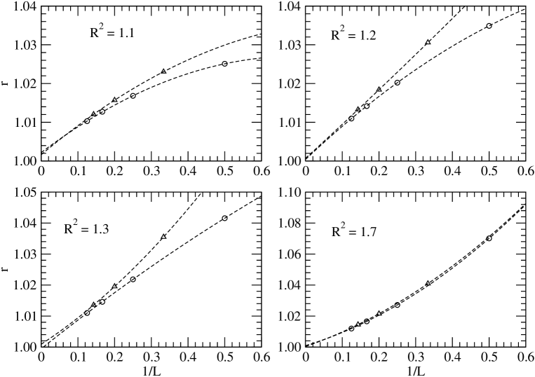
Figure 1: Convergence of the ratio as $L\to\infty$ for four representative values of the compactification radius. Circles and triangles denote the even and odd values of $L$ respectively.

It is clear that the two subsequences with even or odd $L$ belong to different smooth curves and any extrapolation procedure to the $L\to\infty$ limit must take this fact into account. In particular, we shall attempt a polynomial extrapolation in the variable $1/L$ on the two separate curves. Since we have a small number of points, we simply use a quadratic fit of the form

$$r^{\pm}(L,R)=r^{\pm}_{0}(R)+\frac{r^{\pm}_{1}(R)}{L}+\frac{r^{\pm}_{2}(R)}{L^{2}},$$ (45)

where $+(-)$ refers to the subsequence with even (odd) $L$. The results of such a fit are shown in Table (2).

$R^{2}$	$r^{+}_{0}$	$r^{+}_{1}$	$r^{+}_{2}$	$r^{-}_{0}$	$r^{-}_{1}$	$r^{-}_{2}$
1.1	1.00218	0.0715072	-0.051347	1.00163	0.0796027	-0.0460251
1.15	1.00117	0.0834426	-0.0486889	1.00099	0.086692	-0.0218726
1.2	1.00042	0.0894727	-0.0410577	1.00071	0.0867362	0.00863399
1.25	0.999862	0.0927268	-0.0314023	1.0007	0.083104	0.0427123
1.3	0.999438	0.0946927	-0.020853	1.00091	0.0772442	0.0797859
1.34	0.999939	0.0880721	0.000373569	0.999099	0.100666	-0.0158489
1.35	0.999921	0.0879025	0.00329091	0.999045	0.100956	-0.0144504
1.4	0.99988	0.0867754	0.018415	0.998795	0.102482	-0.00801743
2	0.998946	0.101013	0.0686399	0.999802	0.0922072	0.144219

Table 2: Fit of the ratio $r$ with a quadratic function of $1/L$. The fit is done separately on the even and odd subsequences.

The coefficient $r^{+}_{2}$ changes sign at about $R=R^{*}=\sqrt{1.34}$. The change of convexity of the even subsequence can also be seen in Fig. (1). It is clear that at this special radius, the subleading correction $1/L^{2}$ is very small. Therefore, we can consider the associated value of $r_{0}^{+}(R^{*})$ as the best estimate for the ratio $r$ at infinite level. Indeed, we see from the table, that at $R^{*}$, the obtained estimate $r_{0}^{+}(R^{*})=0.999939$ is quite near the theoretical prediction $r=1$ with a difference at the level of $10^{-5}$.

Similar considerations can be done working on the odd subsequence. Indeed, when $|r^{-}_{2}(R)|$ is small, the estimate $r^{-}_{0}$ is nearer $r=1$. The precision is smaller than in the case of the even subsequence because there are only 3 point to be fit.

In conclusion, the above procedure shows the existence of an optimal compactification radius to test the second conjecture. For any degree of accuracy in the level expansion, at $R^{*}$ the subleading corrections in $1/L$ are suppressed and an improvement in the extrapolation to $L\to\infty$ is assured.

3.1 The Marginal Tachyon Mode

As a byproduct of our calculation, we can try to estimate the $R\to 1$ value of the tachyon first harmonic in the lump solution. This is the coefficient $t_{1}$ of the state $c_{1}|1\rangle_{+}$ in the string field solution. The problem is that now we cannot vary $R$ and we must resort to the extrapolation. A sample of data for $t_{1}$ is reported in Table (3)

$R^{2}$	L=2	4	6	8
1.10	0.29707354	0.33624683	0.35166239	0.35971677
1.15	0.32330778	0.35715693	0.36893321	0.37467583
1.20	0.33995093	0.37021406	0.37973651	0.38411374
1.25	0.35139367	0.37925396	0.38730232	0.39080940
1.30	0.35964714	0.38590964	0.39295642	0.39587931
1.35	0.36579239	0.39143043	0.39744044	0.39989409
1.40	0.37047136	0.39547722	0.40095305	0.40310957
1.70	0.38349706	0.40818453	0.41199685	0.41325659
2.00	0.39340980	0.41116312	0.41404162	0.41489224
$R^{2}$	L=3	5	7
1.10	0.31126782	0.34191381	0.35450203
1.15	0.33696675	0.36177155	0.37101530
1.20	0.35296316	0.37411389	0.38134968
1.25	0.36390617	0.38268707	0.38862042
1.30	0.37183202	0.38904484	0.39408725
1.35	0.38428460	0.39469223	0.39856274
1.40	0.38915108	0.39853680	0.40196426
1.70	0.40194383	0.41043369	0.41261409
2.00	0.40620485	0.41309274	0.41461733

Table 3: Marginal tachyon field $|t_{1}|$ computed at various different radii $R$ and levels $L$. The approximation in the evaluation of the Witten action is always $(L,2L)$.

Again, we show in Fig. (2) the behavior of $t_{1}$ as a function of $1/L$ at four representative radii, together with a quadratic fit as before

$$t_{1}^{\pm}(L,R)=t^{\pm}_{1,0}(R)+\frac{t^{\pm}_{1,1}(R)}{L}+\frac{t^{\pm}_{1,2}(R)}{L^{2}}.$$ (46)

We have estimated the extrapolated $t_{1}(R)$ and its theoretical error as

$$\frac{1}{2}(t^{+}_{1,0}+t^{-}_{1,0})\pm\frac{1}{2}(t^{+}_{1,0}-t^{-}_{1,0}).$$ (47)

The result is shown in Fig. (3). We have performed a fit of $t_{1}(R^{2})$ of the form $(a_{0}+a_{1}R^{2})/(1+a_{2}R^{2})$. Our estimate for $t_{1}(R=1)$ is $0.351(5)$.

The quality of the fit is not bad. However, this result depends of course on the choice of the fitting function and also on the rather arbitrary choice of the representation Eq. (47). In our opinion, a safe determination of $t_{1}(R=1)$ would require in our opinion a better accuracy in the level expansion as well as additional analytical information about the $t_{1}$ dependence on $R$ at least in the critical region $R\simeq 1$.

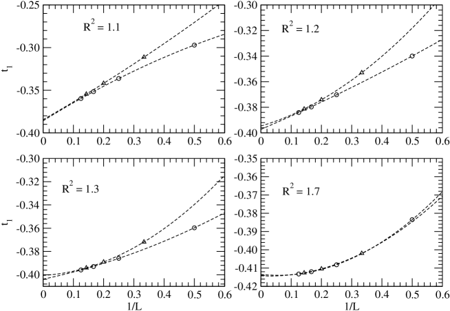
Figure 2: Convergence of the marginal tachyon $t_{1}$ as $L\to\infty$ for four representative values of the compactification radius. Circles and triangles denote the even and odd values of $L$ respectively.

4 Conclusions

In this brief paper we have tried to improve the available accuracy in the check of Sen’s second conjecture predicting the existence of lump solutions in the background of a Dp-brane and representing a lower dimensional D-(p-1) brane. The conjecture asserts that the lump solution energy excess with respect to the non perturbative vacuum precisely matches the D-(p-1) brane tension. The ratio of these two quantities is thus predicted to take the unit value. Previous checks of this prediction confirmed $r=1$ with a precision of about 0.1 %.

We have extended the level expansion of $r$ up to (8, 16). In principle the extension could be further improved . However, we think that it would be convenient to explore also alternative approaches to the $L\to\infty$ limit. In particular, better extrapolation techniques have been shown to be effective in other similar problems in the past [8].

In this spirit, we have analyzed the compactification radius dependence of the ratio $r$, which is expected to be $R$ independent in the infinite $L$ limit. We have shown numerically the existence of an optimal radius $R^{*}\simeq\sqrt{1.34}$ at which the subleading corrections $1/L^{2}$ are suppressed. At this special radius we have obtained the estimate $r=0.999939$ from our moderate (8, 16) data.

Since we explored different radii, it has been natural to analyze the extrapolation of the lump solution in the $R\to 1$ limit. In particular, it is interesting to analyze the first tachyon harmonic which is exactly marginal at $R=1$. Our best estimate is $t_{1}(R=1)=0.351(5)$, but with a rather large theoretical uncertainty.

We hope that this investigation as well as the explicit (8, 16) potential (available on request to the author) will be useful to clarify the precise relation between the D1 $\to$ D0 marginal transition on a circle and the large marginal deformation driven by a Wilson line as investigated in [14, 15].

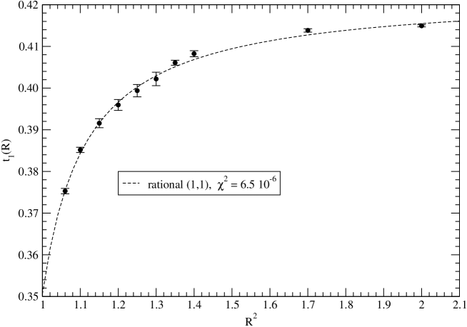
Figure 3: Extrapolated marginal tachyon field $t_{1}(R)$ and rational (1,1) fit.

References

- [1] A. Sen, “Descent relations among bosonic D-branes,” Int. J. Mod. Phys. A 14, 4061 (1999) [arXiv:hep-th/9902105].
- [2] A. Recknagel and V. Schomerus, “Boundary deformation theory and moduli spaces of D-branes,” Nucl. Phys. B 545, 233 (1999) [arXiv:hep-th/9811237]. C. G. . Callan, I. R. Klebanov, A. W. W. Ludwig and J. M. Maldacena, “Exact solution of a boundary conformal field theory,” Nucl. Phys. B 422, 417 (1994) [arXiv:hep-th/9402113]. J. Polchinski and L. Thorlacius, “Free fermion representation of a boundary conformal field theory,” Phys. Rev. D 50, 622 (1994) [arXiv:hep-th/9404008].
- [3] A. Sen, “Tachyon dynamics in open string theory,” arXiv:hep-th/0410103. L. Rastelli, “Open string fields and D-branes,” Fortsch. Phys. 52, 302 (2004). W. Taylor and B. Zwiebach, “D-branes, tachyons, and string field theory,” arXiv:hep-th/0311017. W. Taylor, “Lectures on D-branes, tachyon condensation, and string field theory,” arXiv:hep-th/0301094.
- [4] V. A. Kostelecky and S. Samuel, “The Static Tachyon Potential In The Open Bosonic String Theory,” Phys. Lett. B 207, 169 (1988). V. A. Kostelecky and R. Potting, “Expectation Values, Lorentz Invariance, and CPT in the Open Bosonic String,” Phys. Lett. B 381, 89 (1996) [arXiv:hep-th/9605088].
- [5] A. Sen and B. Zwiebach, “Tachyon condensation in string field theory,” JHEP 0003, 002 (2000) [arXiv:hep-th/9912249].
- [6] W. Taylor, “D-brane effective field theory from string field theory,” Nucl. Phys. B 585, 171 (2000) [arXiv:hep-th/0001201].
- [7] N. Moeller and W. Taylor, “Level truncation and the tachyon in open bosonic string field theory,” Nucl. Phys. B 583, 105 (2000) [arXiv:hep-th/0002237].
- [8] M. Beccaria and C. Rampino, “Level truncation and the quartic tachyon coupling,” JHEP 0310, 047 (2003) [arXiv:hep-th/0308059].
- [9] P. Fendley, H. Saleur and N. P. Warner, “Exact solution of a massless scalar field with a relevant boundary interaction,” Nucl. Phys. B 430, 577 (1994) [arXiv:hep-th/9406125]. J. A. Harvey, D. Kutasov, E. J. Martinec and G. W. Moore, “Localized tachyons and RG flows,” arXiv:hep-th/0111154. J. A. Harvey, D. Kutasov and E. J. Martinec, “On the relevance of tachyons,” arXiv:hep-th/0003101.
- [10] J. A. Harvey and P. Kraus, “D-branes as unstable lumps in bosonic open string field theory,” JHEP 0004, 012 (2000) [arXiv:hep-th/0002117].
- [11] R. de Mello Koch, A. Jevicki, M. Mihailescu and R. Tatar, “Lumps and p-branes in open string field theory,” Phys. Lett. B 482, 249 (2000) [arXiv:hep-th/0003031].
- [12] N. Moeller, A. Sen and B. Zwiebach, “D-branes as tachyon lumps in string field theory,” JHEP 0008, 039 (2000) [arXiv:hep-th/0005036].
- [13] A. Sen, “Universality of the tachyon potential,” JHEP 9912, 027 (1999) [arXiv:hep-th/9911116].
- [14] A. Sen and B. Zwiebach, “Large marginal deformations in string field theory,” JHEP 0010, 009 (2000) [arXiv:hep-th/0007153].
- [15] A. Sen, “Energy momentum tensor and marginal deformations in open string field theory,” JHEP 0408, 034 (2004) [arXiv:hep-th/0403200].
- [16] E. Witten, “Non-commutative Geometry And String Field Theory,” Nucl. Phys. B 268, 253 (1986).
- [17] M. R. Gaberdiel and B. Zwiebach, “Tensor constructions of open string theories. II: Vector bundles, D-branes and orientifold groups,” Phys. Lett. B 410, 151 (1997) [arXiv:hep-th/9707051]. M. R. Gaberdiel and B. Zwiebach, “Tensor constructions of open string theories I: Foundations,” Nucl. Phys. B 505, 569 (1997) [arXiv:hep-th/9705038].
- [18] L. Rastelli and B. Zwiebach, “Tachyon potentials, star products and universality,” JHEP 0109, 038 (2001) [arXiv:hep-th/0006240]. D. Gaiotto and L. Rastelli, “Experimental string field theory,” JHEP 0308, 048 (2003) [arXiv:hep-th/0211012].