Rational foundation of GR in terms of statistical mechanic in the AdS/CFT framework

Abstract:

In this article, we work out the microscopic statistical foundation of the supergravity description of the simplest 1/2 BPS sector in the AdS(5)/CFT(4). Then, all the corresponding supergravity observables are related to thermodynamical observables, and General Relativity is understood as a mean-field theory. In particular, and as an example, the Superstar is studied and its thermodynamical properties clarified.

1 Introduction

The AdS/CFT correspondence is a powerful framework to study the microscopic structure of space-time [1]. In this setting the gravitational field theory can be regarded as a mean-field theory, resulting from a coarse graining of the microscopic degrees of freedom. In this form, the role of General Relativity is more alike to an equation of state, a derived effective theory , that is obtained from thermodynamical arguments. Note that from this point of view, its direct quantization is as useful as the quantization of an effective theory, and therefore has little to tell about the ultraviolet degrees of freedom that have been integrated out. In fact, it was notice in [2] that from generalized Black Hole entropy laws, Einstein equations can be deduce. Of course, this last point does not prove our point of view, but it certainly reinforce it and show its consistency.

In this setting, we have to face the fact that observables in general relativity are all intrinsically thermodynamical, and that our main quest should be to find a statistical mechanics arguments to give a rationale foundation to General Relativity.

In particular, Black Holes (BH) should be seen in the same light. Here General Relativity shows more explicitly its thermodynamical aspects (e.g. the BH thermodynamical laws) and its limits, like the pathological singularities at its core or the possible lost of unitarity. Following the above line of reasoning, we have to revised our concepts of BH physics, to find out up to what extent we can push the classical picture (like for example the concept of event horizon), into quantum process. At this point, we have to make reference to a particular incarnation of this framework, in the work of Mathur et. al. ( see[3] and reference there in), where the actual definition of a BH is replaced by a sort of coarse grained geometry, where the meaningful concept seems to rely on the emergence of semiclassical microstates geometries. Here, the event horizon and basically any classical observable are just a blur picture resulting from a measurement of a system in a mixed state in the underlying ultraviolet partons. Nevertheless, we should also recalled that this particular incarnation is not fully understood and checked for realistic BH, and more work needs to be done to bring it into more firm grounds. In any case, it is clear the BH physics begs for a rational foundation in terms of statistical arguments of the ultraviolet degrees of freedom.

A particulary useful sector in the AdS/CFT duality is the one that deals with the simples 1/2 supersymmetric configurations. In the CFT side it is describe by a Matrix quantum mechanics that can be recast in terms of many non-interacting fermions in a quantum Hall effect, coffined to stay in the lowest Landau level (see [4, 5]). The Gravity side is describe by the LLM construction [6], where only the metric and the Ramond-Ramond 5-form are switched on. The beauty of this sector is that the classical limit of the CFT theory (i.e. the form of the corresponding droplets in phase space) sources the space-time solutions, in a one to one correspondence. Unfortunately this sector does not contain any BH, but a poor relative called superstar [7] (SS), with no horizon and a naked singularity at its center. Nevertheless, the SS develops a horizon as soon as it is perturbed by non bps states, and it has been argue in [8] that it actually grows a small horizon after stringy corrections are taken into account. In any case, this solution is the responds of space-time to a distribution of D3-branes (in this context named Giant gravitons), that has an associated degeneracy of states that scales exponentially with its energy and therefore gives a non vanishing entropy.

Here we study a model, based on statistical mechanics of the dual CFT system of the LLM sector, to give a rational foundation of its thermodynamical properties or as it was formally known, its GR description. For definiteness, we study the statistical properties of all the states in the CFT Hilbert space, of fixed Energy, that source the SS as an example. Therefore we work in the Microcanonical ensemble. To make a connection to the classical phase space we use the phase space formulation of quantum mechanics of Weyl [9]and Wigner [10] and the associated inverse operators of Groenewold [11].

The result of the study are a clear picture of the emergence of the mean-field description, underlying the thermodynamical properties of the SS and in general extendable to the whole 1/2 BPS sector.

We are aware of two works where the SS has been studied using the fermion picture, [8, 12]. In the first work, the entropy of the dual system to the SS is calculated in a particular regime, to conclude that is consistent with the appearance of an stretch horizon (following Mathur ideas), defined by the microstate with lower energy. In the second article, it is shown the the naive Microcanonical ensemble does not reproduced the correct semiclassical density of states and that the definition of the stretch horizon is subtle. Here, we find a solution to the ensemble problem, giving the form of the distribution, leaving open the definition of the will-be stretched horizon.

Also, the idea that General relativity is an effective theory, is really a definition within string theory. Here, we are giving a explicit scenario, with examples, were the quantum nature of the microscopic degrees of freedom are studied and the thermodynamical nature of General Relativity observed with clarity. There are other two works with similar intentions [13, 14]. The first one using a formalism that is different, recovers the semiclassical vacuum density and also propose a method to study less symmetric sectors in the AdS/CFT (i.e. with less supersymmetry). The second is a titanic effort to understand the foundations of GR, and certainly study in detail the SS. Nevertheless, their approach is again different to our approach. In [14] a connection between the semiclassical form of the fermionic droplets and the form of Young diagrams representing the ensemble of fermions is established (basically both are pictorial representations of energy dependent ensembles of states).

The articles [12, 13, 14] appeared while we where at the final stage of this work. There is overlap and we discuss similar matter, although our focus is different. We believe that our point of view is valuable, and adds for a more complete understanding of this matters.

2 Quantum Mechanics, Phase Space and Classical limit

The basic idea we are using, is that the semiclassical limit of the different states of $N$ non-interacting fermions, are the boundary conditions the uniquely defines the dual gravity configuration. To be more precise, in the semiclassical limit fermions have a minimal area of order $\hbar$ in phase space. Due to Pauli exclusion principle, they can not be at the same point, therefore spread forming droplets. This droplets are in turn the boundary data that specifies uniquely the dual supergravity configuration. It is important to make notice that many different quantum states may form the same classical droplet, and in fact, in the correspondence it is used that measurements of order $\hbar$ are not possible to be resolved. This is the essence for the coarse graining picture.

In order to understand the duality, we need to get a grip of the classical limit of the fermion system in term of phase space variables incorporating the notion of ensembles of states, since the supergravity measurements will in general, only define a subspace of the total Hilbert space. To this end, we use Weyl and Wigner formalism, where in short, quantum mechanics is rewritten in term of a phase space operator density.

One particle case

For simplicity, we start with a single particle Hilbert space, that gives a two-dimensional phase space. A particulary useful operator to investigate on thermodynamical properties is the density operator $\hat{\rho}$. For a mixed state in a n-dimensional subspace of the Hilbert space, we have that

$$\hat{\rho}=\sum_{n}P_{n}|\psi_{n}><\psi_{n}|\quad\quad\sum_{n}P_{n}=1,,$$ (2.1)

where the expectation value of an operator $\hat{A}$ is given by $<\hat{A}>=Tr(\hat{A}\hat{\rho})$.

Then, given an operator $\hat{A}$ the Weyl transformation associates to it, a function $A(q,p)$ as follows

$$A(q,p)=\int dy<q+\hbox{${y\over 2}$}|\hat{A}|q-\hbox{${y\over 2}$}>e^{-ipy/\hbar}\,,$$ (2.2)

where the $|q>$ is the usual position basis. Then, the Wigner density is just the Weyl transformation of $\hat{\rho}$,

$$W(q,p)={1\over 2\pi\hbar}\int dy<q+\hbox{${y\over 2}$}|\hat{\rho}|q-\hbox{${y\over 2}$}>e^{-ipy/\hbar}\,,$$ (2.3)

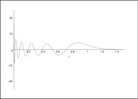
Figure 1: plot for n=10

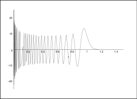
Figure 2: plot for n=40

There are many interesting properties of $W$ that deserved attention but here we will just say that for Harmonic oscillators, its dynamics is identical to the dynamics of the classical Liouville density. On the other hand it is well known that this operator has negative eigenvalues, a feature not very pleasant for a candidate to a classical density. Nevertheless, we are interested in the semiclassical limit of a harmonic oscillator, and here, $W$ behaves much more nicely. Consider the harmonic oscillator, with Hamiltonian $\bar{H}=p^{2}/2m+(mw^{2}/2)q^{2}$, with energy eigenstates $|n>$ and energy levels $E_{n}=\hbar w(n+1/2)$. then $W$ for one of these pure states is given by

$$W(n;q,p)=\left[(-1)^{n}\over\pi\hbar\right]e^{[-2H(q,p)/\hbar w]}L_{(n)}[4H(q,p)/\hbar w]\,,$$ (2.4)

where $L_{(n)}$ is the Laguerre polynomial of order $n$. To study the classical behavior is useful to define the dimensionless quantity $\tau={2H\over\hbar w}=\left(\beta^{2}q^{2}+\hbox{${1\over\hbar^{2}\beta^{2}}$}p^{2}\right)$ with $\beta^{2}={mw\over\hbar}$. Then we have that

$$\lim_{\hbar\rightarrow 0}W(n;p,q)=(1/\pi)\delta(t)$$ (2.5)

This is expected since in this limit $E_{n}\rightarrow 0$. Nevertheless we are interested in a different classical limit where the energy of our states $E$, is kept constant. In this case, we have to send $n\rightarrow\infty$ as $\hbar\rightarrow 0$. This is a more subtle limit and care should be taken to understand what is going on. For large $n$ and small $\hbar$ we get a rapidly oscillatory behavior, and a final lump at the value of the fixed energy $t_{0}=E_{0}/w$ (see fig. 1 and fig.2 where we plot the Wigner density for different values of $n$).

To preform a measurement of an observable $A$, we have to integrate $W\times A$ on phase space. Basically, the oscillatory part of $W$ cancels out, and only the last lump gives a meaningful contribution. Therefore we can write to good approximation that

$$\lim_{Efixed}W(n;p,q)=(1/\pi)\delta(t-t_{0})\,.$$ (2.6)

Summarizing, for a single particle in a harmonic potential, the Wigner density reproduce the desiderate classical limit when $\hbar$ goes to zero and the Energy is fixed constant. In particular we have only consider the energy, and therefore, our classical density defines a ring on phase space. To talk about more localized classical limits in phase space, coherent states should be used. The presented developments are enough for the scope of this work.

Many particles case

Consider now, the case of $N$ fermions. This time, the Hilbert space is the tensor product of $N$ single particle Hilbert spaces, $\mathcal{H}_{total}=\mathcal{H}_{1}\otimes\mathcal{H}_{2}\ldots\otimes\mathcal{H}_{N}$. Due to the Dirac statistics, any physical state has to be anti-symmetric on each single particle Hilbert space. Using the creation and annihilation operators $a^{{\dagger}}_{i},a_{i}$ acting on $\mathcal{H}_{i}$, a basis for the physical states, can be label by a N-dimensional vector $\vec{n}$ where its coordinates $n_{i}$ corresponds to the number of times the creation operator $a^{\dagger}_{i}$ acts on the vacuum. In this notation, anti-symmetrization is understood, where $n_{i}>n_{j}$ if $i<j$ and when written explicitly the Slater determinant of the following form is obtained

$$|\vec{n}>={\det\pmatrix{&({a^{\dagger}_{1}})^{n_{1}}&({a^{\dagger}_{1}})^{n_{2}}&\cdots&({a^{\dagger}_{1}})^{n_{N}}\cr&({a^{\dagger}_{2}})^{n_{1}}&({a^{\dagger}_{2}})^{n_{2}}&\cdots&({a^{\dagger}_{2}})^{n_{N}}\cr&\vdots&;\vdots&;\ddots&;\vdots\cr&({a^{\dagger}_{N}})^{n_{1}}&({a^{\dagger}_{N}})^{n_{2}}&\cdots&({a^{\dagger}_{N}})^{n_{N}}\cr}}|0>.$$ (2.7)

The above notation also has a closed connection to $U(N)$ Young diagrams where each $n_{i}$ is associated to the number of boxes of on the row $"i"$, in a given diagram. Note that each of these states has a definite energy $E_{n}=\hbar w\sum_{i=1}^{N}(n_{i}+1/2)$, and the energy of the fermionic vacuum or Fermi sea is $\hbar w{N^{2}\over 2}$.

Let us write the form of the Wigner density for one of the above states $|\vec{n}>$, following our previous definitions we write

$$W(\vec{n},\vec{q},\vec{p})={1\over 2\pi\hbar}\int(dy)^{N}<\vec{q}+\hbox{${\vec{y}\over 2}$}|\vec{n}><\vec{n}|\vec{q}-\hbox{${\vec{y}\over 2}$}>e^{-i\vec{p}\vec{y}/\hbar}\,,$$ (2.8)

where the integration is taken over an $N$-dimensional space, and therefore $W$ is a function of the vectors $(\vec{q},\vec{p})$.

To have an idea of the form of $W$, let s consider the Fermi vacuum state for $N=2$. In this case the vacuum is given by

$$|1,0>={1\over\sqrt{2}}(a^{{\dagger}}_{1}-a^{{\dagger}}_{2})|0>\quad,\quad<\vec{q}+\hbox{${\vec{y}\over 2}$}|\vec{n}>={\beta\over 2\sqrt{\pi}}\,e^{-{\beta^{2}\over 2}\,\vec{q}^{2}}[H_{1}(\beta q_{1})-H_{2}(\beta q_{2})]$$

and hence, after some algebra we get

$$W(v_{2};\vec{q},\vec{p})=-\left(2\over\pi\hbar\right)e^{-\left(\beta^{2}\vec{q}^{2}+\hbox{${1\over\hbar^{2}\beta^{2}}$}\vec{p}^{2}\right)}\left\{1-\left[\beta^{2}(\Delta q)^{2}+{1\over\hbar^{2}\beta^{2}}(\Delta p)^{2}\right]\right\},$$ (2.9)

where the $v_{2}$ stand for the two-dimensional vacuum and $\Delta a=a_{1}-a_{2}$. At this point, to recover the density function, depending only on one pair of canonical coordinates $(q,p)$, we just have to integrate over the other canonical pairs, since what we want to define, is the probability to measure a fermion, doesn’t matter which one, in a given position in phase space. After integration, with proper care on the anti-symmetrization properties, we get

$$W(v_{2};q,p)={1\over\pi\hbar}\left[e^{-\tau}-e^{-\tau}(1-\,2\tau)\right],$$ (2.10)

where $\tau$ is defined as in the single particle case. The above calculation when generalized to $N$ fermions gives

$$W(v_{N};q,p)={1\over 2\pi\hbar}\sum_{n=0}^{N-1}(-1)^{n}2e^{-\tau}L_{n}(2\tau)$$ (2.11)

where the $v_{2}$ stand for the N-dimensional vacuum. This same expression can be found by a complete different approach, where the quantization program is based on a non-commutative star product $*$ (see for a review with application to this picture [15]). In this framework $W$ has to satisfies the equation

$$W*W(p,q)=W(p,q)$$

where

$$W*W(p,q)=e^{i\hbar/2(\partial_{q1}\partial_{p2}-\partial_{q2}\partial_{p1})}W(q_{1},p_{1})\,W(q_{2},p_{2})|_{(q_{1}=q_{2}=q;p_{1}=p_{2}=p)}.$$

Now, in the classical limit where the higher energy level is kept constant, this Wigner density produces a step function, that translates into a circular droplet in phase space. A insightful way to understand this is from the single particle picture, as follows: The classical limit is taken, in such a way that the higher energy level remains constant i.e. the $\hbar\sim N^{-1}$ while $N\rightarrow\infty$. The last term of the sum in equation (2.11), behaves more and more like a delta function center at the corresponding $\tau_{0}$, but the other terms also tend to delta functions, only that they are centered at lower $\tau_{i}$, forming a chain of delta functions, one after the other. In the large $N$ limit, they become indistinguishable from a step function, since we can not resolve distances of order $1/N$ (see fig. 3 and fig .4).

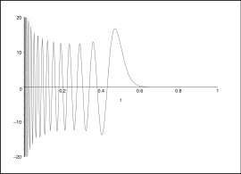
Figure 3: The delta distribution is center at $\tau=30/60$

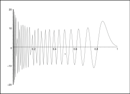
Figure 4: The delta distribution is center at $\tau=54/60$

Therefore we see the emergence of the vacuum configuration out of the quantum theory in a very explicit way. Each term of the sum should be identified with a given fermion, since in the classical limit these terms collapse into $N$ delta functions, forming a circular droplet out of infinitesimal concentric rings.

At this point, we are ready to write the form of the Wigner function, for general pure states of the form $|\vec{n}>$. The result is clearly a sum of $N$ terms of the form $e^{-\tau}L_{n_{i}}(2\tau)$ where each one has the same coefficient, i.e.

$$W(\vec{n};q,p)={1\over 2\pi\hbar}\sum_{n_{i}}(-1)^{n_{i}}2e^{-\tau}L_{n_{i}}(2\tau)\,.$$ (2.12)

This picture is in complete agreement with the slater determinant picture studied in [4, 5]. For example, the Wigner density of a giant graviton with energy $m$, growing in AdS (corresponding to a schur polynomial in the symmetric representation of $S_{N}$ of degree $m$ with vector $\vec{n}_{m}=(m+N-1,N-2,\ldots,0)$) has the expected form

$$W(\vec{n}_{m};q,p)={1\over 2\pi\hbar}\sum_{n=0}^{N-2}(-1)^{n}2e^{-\tau}L_{n}(2\tau)+{1\over 2\pi\hbar}(-1)^{N-1}2e^{-\tau}L_{m+N-1}(2\tau)$$ (2.13)

which also agrees with the picture of concentric rings, exited above the fermi sea level.

Another very interesting feature that we point out, is that the $N$-Fermion Wigner function can be understood as a mixed state of a single particle, where the coefficient of the sum in equation (2.11), correspond to the probability of occurrence of each single pure state with a funny normalization.

$$W(v_{N};q,p)=\sum_{n=0}^{\infty}P_{n}{1\over\hbar}(-1)^{n}e^{-\tau}L_{n}(2\tau)\quad,\quad\sum_{n=0}^{\infty}P_{n}=N\,.$$ (2.14)

Summarizing, as in the single particle case, we have been able to reproduce the classical limit of the Wigner density for the $N$-fermion system. In this case, The final form of the density is obtain by integrating out the extra $(N-1)$ canonical pair of coordinates $(q_{i},p_{i})$. The resulting function is the superposition of $N$ single particles in different eigenstates of the energy, defined by either its Young diagrams, or the vector $\vec{n}$. We have reproduced in the classical limit, the vacuum configuration corresponding to the round droplet, and also all the droplets form by the superposition of concentric rings. Also, the above pure states can be reinterpreted as a Wigner density of a mixed state for a single particle. This interpretation justifies and translates into the superposition properties characteristic of the GR regime, where the solutions are found by superposition of different droplets configurations.

3 Statistical analysis and GR

One of the more interesting outcomes of the previous analysis was that the Wigner function for $N$ Fermions, can be reinterpreted as a Wigner function of a single particle in a mixed state. As long a we are in the quantum regime this is no more than a nice observation. Nevertheless, as soon as we take the classical limit, and the number of fermions grows, nearby fermions forms indistinguishable drops, and many different initial configurations result in the same final drop. Therefore, we lose the trace of the true quantum state, to end up with a classical density that only selects subspaces in the original Hilbert space. At this point, due to our ignorance, we rather have an ensemble of states or a mixed state. The fact that we interpret Wigner as a single particle mixed state makes this transition smooth since or statistical Wigner function of the classical system will be of the same form, with a infinite sum or an integral if you prefer.

Therefore our proposal is that the thermodynamical nature of GR comes about due to the coarse graining of the classical limit, that at the end, translates in our incapability to resolve the specific quantum state that produces the classical observable.

To test this conjecture, we study the nearest classical soliton in this 1/2 BPS sector of supergravity to a BH, the superstar (SS).

Superstar as a mixed state

The SS solution has been much studied lately, here we just need that it is a 1/2 BPS solution with energy $E=N^{2}Q/2L=\Delta/L$, with a naked singularity an the center of $AdS?5$, that extends all over $S^{5}$ and that has been interpreted as the space-time responds of a particular distribution of giant gravitons [7].

From the point of view of the LLM construction, the above solution corresponds to a circular drop of larger radius $R_{Q}$ than the vacuum radius $R_{0}$, forcing the classical fermion density $\rho_{c}$, to attain lower values than 1. To be more exact, $R_{0}^{2}=2\hbar N$, and $R_{Q}^{2}=2\hbar N(1+Q)$, in fact we have that

$$\rho_{c}={1\over 2\pi\hbar(1+Q)}\theta(r^{2}-R^{2}_{Q})\,.$$

In this case the drop is said to be grey in contrast to black drops, where $\rho_{c}=1$.

We would like to see this gray density as the outcome of a Wigner density in the Microcanonical ensemble. Hence we write that

$$\hat{\rho}=\sum_{i=1}^{d}P_{i}|\vec{n}_{\Delta}><\vec{n}_{\Delta}|\quad,\quad\sum_{i=1}^{d}P_{i}=1$$ (3.1)

where $|\vec{n}_{\Delta}>$ are $N$-Fermion eigenstate of the Hamiltonian introduced before, with total energy $\Delta$ and degeneracy $d$.

Equiprobable distribution

The particular form of $P_{i}$, depends on the character or the statistical nature of the mixed state in the ensemble. A very natural option will be the case where all $P_{i}$ are equal, i.e.

$$P_{i}=\left({1\over d}\right)\,,$$

nevertheless, it is not difficult to see that this ”natural guess ” can not be correct for al values of $Q$. To show this, consider the case when $Q<N$, and make notice that when Wigner density is computed, we get the following structure

$$W(\vec{n}_{\Delta},q,p)={1\over 2\pi\hbar}\sum_{m=0}^{N-\Delta}(-1)^{m}2e^{-\tau}L_{2\tau}+{1\over 2\pi\hbar}\left({1\over d}\right)\sum_{d}\delta W$$ (3.2)

where $\delta W$ is the contribution of the exited states over the Fermi sea of level $N-\Delta$ that is left unperturbed. In this case the corresponding classical density $\rho_{c}$ would rather be a black droplet with an external ring of variable density (not equal 1).

What is going on, is that in the equiprobable case, there are many possible ways to have a large number of giant gravitons say $m$, with an energy of the same range, in comparison to the case where we have a small number of very energetic giants or a large number of giants with little energy. Basically, this tails of the probability density spoil the result. What we need is a distribution where the states that appear, have the same order of energy and number of Giants. In terms of Young diagrams, we need an ensemble of almost triangular diagrams.

$$\btexdraw\drawdim cm\move(0.5)\lvec(4.5)\move(00)\lvec(40)\move(0-.5)\lvec(3-.5)\move(0-1.5)\lvec(2.2-1.5)\move(0-2)\lvec(2.2-2)\move(0-2.5)\lvec(1.5-2.5)\move(0.5)\lvec(0-2.5)\move(.5-2.5)\lvec(.5-1.5)\move(.5-.5)\lvec(.5.5)\move(1-.5)\lvec(1.5)\move(1-.0)\lvec(1.5)\move(1.5-.0)\lvec(1.5.5)\move(4.0)\lvec(4.5)\move(3-.5)\lvec(30)\move(2.2-2.0)\lvec(2.2-1.5)\move(1.5-2)\lvec(1.5-2.5)\move(1.8.25)\fcir f:0r:.01\move(2.0.25)\fcir f:0r:.01\move(2.2.25)\fcir f:0r:.01\move(2.4.25)\fcir f:0r:.01\move(2.6.25)\fcir f:0r:.01\move(2.8.25)\fcir f:0r:.01\move(2.8.25)\fcir f:0r:.01\move(1.2-.25)\fcir f:0r:.01\move(1,4-.25)\fcir f:0r:.01\move(1.6-.25)\fcir f:0r:.01\move(1.8-.25)\fcir f:0r:.01\move(2-.25)\fcir f:0r:.01\move(.6-1.75)\fcir f:0r:.01\move(.8-1.75)\fcir f:0r:.01\move(1-1.75)\fcir f:0r:.01\move(.6-2.25)\fcir f:0r:.01\move(.8-2.25)\fcir f:0r:.01\move(.7-.6)\fcir f:0r:.01\move(.7-.8)\fcir f:0r:.01\move(.7-1)\fcir f:0r:.01\move(.7-1.2)\fcir f:0r:.01\move(.7-1.4)\fcir f:0r:.01\htext(3.5.1){n_{1}}\htext(2.5-.4){n_{2}}\htext(1.2-1.9){n_{N-1}}\htext(.9-2.4){n_{N}}\etexdraw$$

Classical densities and the Groenewold operator

In order to check our conclusions on the form of the mixed state representing the SS, we use the embedding of classical functions into quantum mechanic operators, develop by Groenewold [11]. Basically, to define this quantization method, it is used the fact that the Weyl map of equation (2.2) has a well defined inverse map. Then, given a classical density $\rho_{c}$ the associated operator density is defined as follows

$$\hat{\rho}=\int{dpdq\,\rho_{c}}\,\hat{\Delta}(q,p)\quad\hbox{where}\quad\hat{\Delta}(q,p)=e^{i(q\hat{p}-p\hat{q})}\,\hat{P}\,e^{-i(q\hat{p}-p\hat{q})}$$ (3.3)

and $\hat{P}$ is the parity operator.

In this formalism, the calculation of expectation values corresponding to classical average, takes the familiar quantum mechanic form $Tr(\hat{A}\hat{\rho})$. Also, it is easy to prove that for the Hilbert space basis $\{|n>\}$ corresponding to eigenfunctions of the Hamiltonian of the single particle, $\hat{\rho}$ is diagonal i.e. $<m|\hat{\rho}|n>=\delta_{(m,n)}\lambda_{n}$.

Consider in particular, the form of the SS density in the LLM framework,

$$\rho_{c}=\left\{\begin{array}[]{cc}{N\over(\pi R_{Q}^{2})}&\quad r^{2}<R_{Q}^{2}\\ 0&\quad r^{2}>R_{Q}^{2}\end{array}\right.$$ (3.6)

where by definition, integrating over the phase space gives the total number of particles $N$. To make a clear connection with previous results we recall that the Hamiltonian of a Harmonic oscillator can be written as $H=wr^{2}/2$, where $r^{2}=\hbar\tau$ and we also define $\tau_{Q}=\hbar R_{Q}^{2}$ to obtain

$$\rho_{c}=\left\{\begin{array}[]{cc}{N\over\pi\hbar\tau_{Q}}&\;\;\tau<\tau_{Q}\\ 0&\quad\tau>1\end{array}\right.$$ (3.9)

Then, it is not difficult to compute the eigenvalues of $\hat{\rho}$ when expressed in terms of energy eigenvectors $|n>$, obtaining

$$<m|\hat{\rho}|n>=\left\{\begin{array}[]{cc}{2N(-1)^{m}\over\tau_{Q}}\int_{0}^{\tau_{Q}}d\tau\,[e^{-\tau}L_{(n)}(2\tau)]&\quad m=n\\ \\ 0&\quad m\neq 0\end{array}\right.$$ (3.13)

That should be plug in the final form of $\hat{\rho}$,

$$\hat{\rho}=\sum_{n=0}^{\infty}\lambda_{n}|n><n|$$ (3.14)

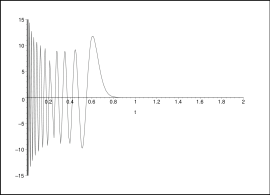
Figure 5: The delta distribution is center at $\tau=26/40$ and hence since in this normalization we integrate up to 1, the integral is not zero

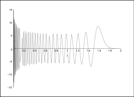
Figure 6: The delta distribution is center at $\tau=66/40$, and the integration gives zero

At this point, it is important to note that $\lambda_{n}$ has a very interesting behavior. For large N, $\lambda_{n}$ approaches zero if $n>N(1+Q)$! and approaches $1/(1+Q)$ if $n<N(1+Q)$. The reason behind this behavior is that the integrand of equation (3.13) tends to $1/(1+Q)$ times the delta function with support in the interval $(0,1)$ if $n<N(1+Q)$ and out of the interval if $n>N(1+Q)$ (see fig. 5 and fig. 6).

Summarizing, We have embedded the classical density for the SS into a single particle quantum mechanic system. We have found that the corresponding density operator is given by a mixed state that is built using the hole tower of states $|n>$. Nevertheless, out of the this infinite set of $\lambda_{n}$, only those that have $n<N(1+Q)$, give a sizable contribution. Hence we can approximate our density operator as follows,

$$\hat{\rho}\simeq\sum_{n=0}^{N(1+Q)}{1\over(1+Q)}|n><n|$$ (3.15)

Therefore, using our result of the previous sections that the density operator of a single particle can be understood as the density operator of N-fermions, we have found the density operator of the SS, has as expected the form of a statistical ensemble, that does not correspond to the equiprobable ansatz. Note that, all the energy levels are populated with the same probability in the single particle picture!, and that doest not corresponds to an equiprobable ensemble in the N-fermion picture, but to a triangular young diagram!.

4 Discussion

In this work adopt the perspective that GR is a mean-field approximation of the microscopic structure defined by the true ultraviolet degrees of freedom. In this approach, GR observables are thermodynamical in nature, an should be understood in terms of statistical mechanics of the ultraviolet degrees of freedom.

As an example of the above ideas, we focus on the simplest 1/2 BPS sector of the $AdS_{5}/CFT$ duality. Here due to the simplicity of the CFT sector, we are able to study the corresponding statistical mechanics to give a rational foundation to the GR dual observables.

We found necessary to use Weyl and Wigner formalism to incorporate the phase-space picture into the quantum mechanics formalism. In particular we found that the Wigner density correspondent to a $N$-fermions pure state, can be understood as a mixed state of a single particle. Then, all types of Wigner densities corresponding to pure or mixed states can be recast in terms of mixed states of the single particle.

Classical limit is surprisingly easy to take, the unpleasant features of the Wigner density cancel out, showing a clear picture where the classical point particles emerge as delta functions. In particular we recover in this form, the vacuum configuration, giant gravitons and in general al the previous known configurations single out in GR that where built out of concentric rings.

As a bonus of the above construction, we explain why the GR description is linear in the droplets. Basically, each drop is related to classical limit of mixed state, and the Wigner density of the system is the sum or linear superposition of all mixed states.

At last, we have analyzed the SS solution of GR from the statistical mechanics point of view. We found that the corresponding mixed state, is not describe by an equiprobable distribution of states with fixed energy, but rather a distribution where only those states with almost triangular Young diagram are present. Nevertheless, when the distribution is rewritten in terms of the single particle states, we obtain an equiprobable distributions as final result. It seems to us, that in this sector the theory is telling that the natural variables to be used are the single particle ones.

The sector study in this work, has received some attention lately, in particular research on its quantum structure and consequences to the GR picture result in a chronology protection mechanism based on the Pauli exclusion principle [16]. Also, the direct quantization of the LLM solutions has been studied. Here, the collective coordinate quantization can be reproduced by the D3-branes effective action in the LLM background [17]. A more canonical scenario was considered in [18], where a pure GR approach with no mention to stringy tools was undertaken. In this case, the bosonization of the underlying microscopic femionic theory is recovered. Nevertheless, from our point of view, it is hard to see how the full quantum structure would be recovered once the coarse graining is done in this case not to mention in other more general cases. At last ”Bubbling AdS” have been exported to other systems, like the D1/D5 case [19], and again has brought more understanding on the quantum structure of GR [20]. Unfortunately, in this case we do not have a good idea of what is the equivalent of the $N$-fermions picture for the microscopic degrees of freedom. Definitively more study should be done in this directions.

We believe that this work is ”a nice example” where the underlying structure of space-time is exposed, and that with some luck, nature works in a similar fashion. In any case, there are plenty of things to uncover in this context, not to talk about the general case.

References

- [1] J. M. Maldacena, Adv. Theor. Math. Phys. 2 (1998) 231 [Int. J. Theor. Phys. 38 (1999) 1113] [arXiv:hep-th/9711200].
- [2] T. Jacobson, Phys. Rev. Lett. 75 (1995) 1260 [arXiv:gr-qc/9504004].
- [3] O. Lunin, S. D. Mathur and A. Saxena, Nucl. Phys. B 655 (2003) 185 [arXiv:hep-th/0211292]. O. Lunin and S. D. Mathur, Nucl. Phys. B 642 (2002) 91 [arXiv:hep-th/0206107]. O. Lunin and S. D. Mathur, Nucl. Phys. B 623 (2002) 342 [arXiv:hep-th/0109154].
- [4] S. Corley, A. Jevicki and S. Ramgoolam, Adv. Theor. Math. Phys. 5 (2002) 809 [arXiv:hep-th/0111222]. D. Berenstein, JHEP 0407 (2004) 018 [arXiv:hep-th/0403110].
- [5] M. M. Caldarelli and P. J. Silva, JHEP 0408 (2004) 029 [arXiv:hep-th/0406096].
- [6] H. Lin, O. Lunin and J. Maldacena, JHEP 0410 (2004) 025 [arXiv:hep-th/0409174].
- [7] R. C. Myers and O. Tafjord, JHEP 0111 (2001) 009 [arXiv:hep-th/0109127].
- [8] N. V. Suryanarayana, arXiv:hep-th/0411145.
- [9] Weyl, H., (Dover, New York) 1930, p. 274.
- [10] Wigner E. P. Physi. Rev. 40 (1932) 749
- [11] Groenewold, H. Phisica, 12 (1946) 405.
- [12] P. G. Shepard, arXiv:hep-th/0507260.
- [13] D. Berenstein [arXiv:hep-th/0507203].
- [14] V. Balasubramanian, J. de Boer, V. Jejjala and J. Simon, arXiv:hep-th/0508023.
- [15] A. Dhar, arXiv:hep-th/0505084.
- [16] M. M. Caldarelli, D. Klemm and P. J. Silva, arXiv:hep-th/0411203.
- [17] G. Mandal, arXiv:hep-th/0502104.
- [18] L. Gran, L. Maoz, J. Marsano, K. Popadodimas and V.S.Rycohkov [arXiv:hep-th/0505079]
- [19] J. T. Liu, D. Vaman and W. Y. Wen, arXiv:hep-th/0412043. D. Martelli and J. F. Morales, JHEP 0502 (2005) 048 [arXiv:hep-th/0412136]. J. T. Liu and D. Vaman, arXiv:hep-th/0412242.
- [20] M. Boni and P. J. Silva, arXiv:hep-th/0506085.