Thermal Operator Representation of Finite Temperature Graphs

Abstract

Using the mixed space representation $(t,\vec{p}\,)$ in the context of scalar field theories, we prove in a simple manner that the Feynman graphs at finite temperature are related to the corresponding zero temperature diagrams through a simple thermal operator, both in the imaginary time as well as in the real time formalisms. This result is generalized to the case when there is a nontrivial chemical potential present. Several interesting properties of the thermal operator are also discussed.

I Introduction

In a series of recent papers Espinosa:2003af ; Espinosa:2005gq ; Blaizot:2004bg , it was shown for theories involving scalar as well as fermion fields that every graph in momentum space at finite temperature in the imaginary time formalism kapusta:book89 ; lebellac:book96 ; das:book97 is related to the corresponding graph of the zero temperature Euclidean field theory through a thermal operator which has a rather simple form. Namely, for a scalar $N$-point amplitude (at any loop) at temperature $T$ one has

$$\int\prod_{i=1}^{I}\frac{\mathrm{d}^{3}k_{i}}{(2\pi)^{3}}\ \prod_{v=1}^{V}{(2\pi)^{3}}\delta^{(3)}_{v}(k,p)\,\gamma_{N}^{(T)}=\int\prod_{i=1}^{I}\frac{\mathrm{d}^{3}k_{i}}{(2\pi)^{3}}\ \prod_{v=1}^{V}{(2\pi)^{3}}\delta^{(3)}_{v}(k,p)\,{\cal O}^{(T)}\ \gamma_{N}^{(T=0)},$$ (1)

where

$${\cal O}^{(T)}=\prod_{i=1}^{I}\left(1+n_{i}(1-S_{i})\right).$$ (2)

Here $I$ characterizes the total number of internal propagators and $V$ denotes the total number vertices in the graph (with the usual relation for the number of loops $L=I-V+1$), $n_{i}=n(E_{i})$ corresponds to the thermal distribution associated with the internal propagator carrying energy $E_{i}=\sqrt{\vec{k}_{i}^{\ 2}+m^{2}}$ and $S_{i}=S(E_{i})$ is a reflection operator that changes $E_{i}\rightarrow-E_{i}$ (namely, it gives a term with $E_{i}\rightarrow-E_{i}$). We denote the internal and the external three momenta of a graph generically by $(\vec{k},\vec{p}\ )$ respectively and $\delta_{v}^{(3)}(k,p)$ enforces the appropriate three momentum conservation at the vertex $v$. For simplicity, we have included in (1) a delta function which reflects the overall conservation of the external three momenta. Furthermore, $\gamma_{N}^{(T=0)}$ represents the zero temperature graph in momentum space obtained from the Euclidean field theory. This remarkable result is, of course, calculationally quite useful since the worrisome sum over the internal discrete energy values (particularly at higher loops) has already been reduced to evaluating zero temperature energy integrals. More than that, this allows us to study many questions of interest at finite temperature such as Ward identities, analyticity braaten ; frenkel more directly. The original proof of this result in momentum space Espinosa:2005gq ; Blaizot:2004bg however, is quite involved and uses regularization procedures that obscure the origin of such a relation. Furthermore, the proof leaves one with the feeling that such a relation is particular to the imaginary time formalism. In this paper, we discuss a simpler proof of the thermal operator representation both in the imaginary time formalism kapusta:book89 ; lebellac:book96 ; das:book97 as well as in the real time formalisms das:book97 . Furthermore, we also extend this relation to the case when there is a nontrivial chemical potential lebellac:book96 and point out various interesting aspects of this relation.

At finite temperature, it is already noted that simplifications arise when one works not in the energy-momentum space, but rather in a mixed space where energy has been Fourier transformed das:book97 ; Bedaque:1993fa ; Das:1997gg . We exploit this feature to give a simpler derivation of the thermal operator representation in both imaginary time and the real time formalisms with and without a chemical potential. In this paper, we will discuss in detail theories involving scalar fields only to bring out the essential underlying features. The remarkable feature of the thermal operator relation, in such a representation, is that while the finite temperature graph depends on

$$\gamma_{N}^{(T)}=\gamma_{N}^{(T)}(T,E_{i},\tau_{\alpha}),$$ (3)

where $\tau_{\alpha},\alpha=1,2,\cdots,N$ represent the external time coordinates of the graph, the thermal operator depends only on $(T,E_{i})$ but not on the external time coordinates (the zero temperature graph depends on $(E_{i},\tau_{\alpha})$ but not on $T$). As a result, the time derivative operator (with respect to external times) commutes with the thermal operator and the discussion of our results holds equally well for theories with fermions as well as Yang-Mills fields which we will discuss in detail in a separate publication. Our paper is organized as follows. In section II, we first discuss the thermal operator representation in the imaginary time formalism without a chemical potential and then with a nontrivial chemical potential. In this section, we also point out various properties of the thermal operator which are quite interesting. In section III, we derive the thermal operator representation in the closed time path formalism das:book97 ; Schwinger:1961qe ; Bakshi:1962dvKeldysh:1964ud , again with and without a chemical potential, where the general proof is really much simpler than the imaginary time formalism. In section IV, we discuss the thermal operator representation for a general time contour, that includes the case of thermofield dynamics das:book97 ; umezawa:1982nv , where the thermal operator, in general, is not as simple as in the imaginary time and the closed time path formalisms. We conclude with a brief summary of our results in section V.

II Imaginary Time Formalism

Let us consider a massive real scalar field theory in Euclidean space. In this case, we know that the zero temperature propagator in momentum space is given by

$$\Delta^{(T=0)}(p_{E},E)=\frac{1}{p^{2}+m^{2}}=\frac{1}{p_{E}^{2}+E^{2}},$$ (4)

where we have defined

$$E=\sqrt{\vec{p}^{\ 2}+m^{2}}.$$ (5)

The energy variable can now be Fourier transformed to give the propagator in the mixed space at zero temperature to be

$$\Delta^{(T=0)}(\tau,E)=\int\frac{\mathrm{d}p_{E}}{2\pi}\ \frac{e^{-ip_{E}\tau}}{p_{E}^{2}+E^{2}}=\frac{1}{2E}\left[\theta(\tau)e^{-E\tau}+\theta(-\tau)e^{E\tau}\right],\quad-\infty\leq\tau\leq\infty.$$ (6)

At finite temperature in the imaginary time formalism (we will set the Boltzmann constant to unity for simplicity), the propagator in the momentum space has the same form as in (4) with $p_{E}=2\pi kT$ where $k$ is an integer. In this case, the Fourier transform of the propagator leads to

$$\Delta^{(T)}(\tau,E)=T\sum_{k}\frac{e^{-i2\pi kT\tau}}{(2\pi kT)^{2}+E^{2}}=\frac{1}{2E}\left[\left(\theta(\tau)+n(E)\right)e^{-E\tau}+\left(\theta(-\tau)+n(E)\right)e^{E\tau}\right]$$

$$\quad=\frac{1}{2E}\left[\theta(\tau)\left\{(1+n(E))e^{-E\tau}+n(E)e^{E\tau}\right\}+\theta(-\tau)\left\{n(E)e^{-E\tau}+(1+n(E))e^{E\tau}\right\}\right],\quad-\frac{1}{T}\leq\tau\leq\frac{1}{T},$$ (7)

which is symmetric under $\tau\rightarrow-\tau$. It is important to recognize that, in the imaginary time formalism, time is rotated to the negative imaginary axis and lies between the interval $(0,\frac{1}{T})$ so that the propagator (being a difference of time coordinates) is defined only within the interval $(-\frac{1}{T},\frac{1}{T})$. Furthermore, let us note that, in this mixed space representation, the thermal propagator (7) can be naturally written as the sum of a zero temperature part and a finite temperature part much like in the real time formalisms das:book97

$$\Delta^{(T)}(\tau,E)=\Delta^{(T=0)}(\tau,E)+\overline{\Delta}(\tau,E),$$ (8)

where the finite temperature part has the form

$$\overline{\Delta}(\tau,E)=\frac{n(E)}{2E}\left(e^{-E\tau}+e^{E\tau}\right).$$ (9)

Furthermore, we note that both the zero temperature propagator (6) and the finite temperature propagator (7) satisfy the same equation

$$\left(\frac{\partial^{2}}{\partial\tau^{2}}-E^{2}\right)\Delta(\tau,E)=-\delta(\tau),$$ (10)

but the finite temperature propagator satisfies the periodicity condition

$$\Delta^{(T)}(\tau<0,E)=\Delta^{(T)}(\tau+\frac{1}{T},E),$$ (11)

following from the KMS condition Kubo:1957xxMartin:1959jp . It follows, therefore, that $\overline{\Delta}$ in (8) satisfies the homogeneous equation

$$\left(\frac{\partial^{2}}{\partial\tau^{2}}-E^{2}\right)\overline{\Delta}(\tau,E)=0,$$ (12)

and is responsible for incorporating the periodicity condition (11).

It follows now from the forms of the propagators in (6) and (7) that we can write

$$\Delta^{(T)}(\tau,E) = \left(1+n(E)(1-S(E))\right)\Delta^{(T=0)}(\tau,E)$$ (13)

$$= {\cal O}^{(T)}(E)\,\Delta^{(T=0)}(\tau,E),\quad-\frac{1}{T}\leq\tau\leq\frac{1}{T},$$

where we note that the basic thermal operator ${\cal O}^{(T)}(E)$ is independent of the time coordinate of the propagator. As we will see, this basic factorization of the finite temperature propagator in terms of a thermal operator (that contains all the temperature dependence, but no time) and the zero temperature propagator (which carries all the time dependence) is at the heart of the thermal operator representation of any finite temperature graph. Given the factorization in (13), it immediately follows that any one loop graph with $N$ external lines (see figure 1) would lead to the thermal operator representation (we consider the $\phi^{3}$ theory for simplicity, neglect the overall coupling constants, assume that all momenta are incoming and identify $k_{N+1}=k_{1},p_{N+1}=p_{1}$)

Figure 1: One loop diagram in the $\phi^{3}$ theory with $N$ external time coordinates.

$$\int\prod_{i=1}^{N}{\mathrm{d}^{3}k_{i}}\ \delta^{(3)}(k_{i}-k_{i+1}+p_{i+1})\gamma_{N}^{(T)}$$

$$\quad=\int\prod_{i=1}^{N}{\mathrm{d}^{3}k_{i}}\ \delta^{(3)}(k_{i}-k_{i+1}+p_{i+1})\Delta^{(T)}(\tau_{1}-\tau_{2},E_{1})\cdots\Delta^{(T)}(\tau_{N}-\tau_{1},E_{N})$$

$$\quad=\int\prod_{i=1}^{N}{\mathrm{d}^{3}k_{i}}\ \delta^{(3)}(k_{i}-k_{i+1}+p_{i+1})\prod_{i=1}^{N}\left(1+n_{i}(1-S_{i})\right)\Delta^{(T=0)}(\tau_{1}-\tau_{2},E_{1})\cdots\Delta^{(T=0)}(\tau_{N}-\tau_{1},E_{N})$$

$$\quad=\int\prod_{i=1}^{N}{\mathrm{d}^{3}k_{i}}\ \delta^{(3)}(k_{i}-k_{i+1}+p_{i+1}){\cal O}^{(T)}\gamma_{N}^{(T=0)},$$ (14)

where we have identified

$${\cal O}^{(T)}=\prod_{i=1}^{N}{\cal O}^{(T)}(E_{i})=\prod_{i=1}^{N}\left(1+n_{i}(1-S_{i})\right).$$ (15)

Similarly, the thermal operator representation immediately follows from the factorization of the propagator (13) for any higher loop graph where all the vertices have only external times (no internal vertices present). It is obvious, for example, in the case of the graphs shown in figure 2 in the $\phi^{4}$ theory.

Figure 2: Two loop diagrams in the $\phi^{4}$ theory without internal time coordinates.

The difficulty in establishing the thermal operator representation for an arbitrary graph arises when there are internal vertices present for which the internal time coordinates have to be integrated over all allowed values. For example, in the $\phi^{3}$ theory the self-energy graph at two loops can have diagrams containing internal vertices of the form shown in figure 3 ($\tau,\tilde{\tau}$ in this case correspond to internal time coordinates that have to be integrated over the allowed values).

Figure 3: Two loop self-energy diagrams in the $\phi^{3}$ theory with internal time coordinates $\tau,\tilde{\tau}$.

Keeping in mind our earlier comments, we note that at finite temperature, the time integration goes over

$$\int_{0}^{\frac{1}{T}}\mathrm{d}\tau,$$ (16)

while in zero temperature graphs, the internal time needs to be integrated over

$$\int_{-\infty}^{\infty}\mathrm{d}\tau,$$ (17)

and it is not clear a priori how the range of integration (16) can be extended to (17) in order to establish the thermal operator relation. Furthermore, the finite temperature propagator is only defined in the interval $(-\frac{1}{T},\frac{1}{T})$, and it is not clear if it can be analytically continued to other regions (preliminary analysis indicates it cannot be done so consistently). Before giving a general proof that such an extension of the range of integration can, in fact, be made, let us work out a simple example to bring out some of the essential features.

Let us first consider the product of $N$ propagators with a common time that is being integrated, namely,

$$I_{1}=\int_{0}^{\frac{1}{T}}\mathrm{d}\tau\prod_{i=1}^{N}\Delta^{(T)}(\tau-\tau_{i},E_{i}),$$ (18)

where $\tau_{i},i=1,2,\cdots,N$ are assumed to be external times that lie between the interval $(0,\frac{1}{T})$. Using (13), we can write the above expression also as

$$I_{1} = \prod_{i=1}^{N}\left(1+n_{i}(1-S_{i})\right)\int_{0}^{\frac{1}{T}}\mathrm{d}\tau\prod_{i=1}^{N}\Delta^{(T=0)}(\tau-\tau_{i},E_{i})$$ (19)

$$= \prod_{i=1}^{N}\left(1+n_{i}(1-S_{i})\right)\int_{-\infty}^{\infty}\mathrm{d}\tau\prod_{i=1}^{N}\Delta^{(T=0)}(\tau-\tau_{i},E_{i})-\overline{I}_{1},$$

where we have defined

$$\overline{I}_{1}=\prod_{i=1}^{N}\left(1+n_{i}(1-S_{i})\right)\left[\int_{-\infty}^{0}\mathrm{d}\tau\prod_{i=1}^{N}\Delta^{(T=0)}(\tau-\tau_{i},E_{i})+\int_{\frac{1}{T}}^{\infty}\mathrm{d}\tau\prod_{i=1}^{N}\Delta^{(T=0)}(\tau-\tau_{i},E_{i})\right].$$ (20)

We note here that it is because the basic thermal operator in the factorization of the propagator is independent of the time coordinate that it can be taken out of the time integral. Furthermore, although the finite temperature propagator cannot be extended beyond its domain, once we have extracted the thermal operators, the zero temperature propagators are defined on the entire real axis, a fact which we have used in the above. Since the external times satisfy $0\leq\tau_{i}\leq\frac{1}{T}$, using the definition of the zero temperature propagator in (6) the integrals in the bracket above can be evaluated in a simple manner and lead to

$$= \left(\prod_{i=1}^{N}\frac{1}{2E_{i}}\right)\left(\int_{-\infty}^{0}\mathrm{d}\tau\ e^{\sum_{i}E_{i}(\tau-\tau_{i})}+\int_{\frac{1}{T}}^{\infty}\mathrm{d}\tau\ e^{-\sum_{i}E_{i}(\tau-\tau_{i})}\right)$$ (21)

$$= \left(\prod_{i=1}^{N}\frac{1}{2E_{i}}\right)\frac{1}{\sum_{i}E_{i}}\left(e^{-\sum_{i}E_{i}\tau_{i}}+e^{-\sum_{i}\frac{E_{i}}{T}}\times e^{\sum_{i}E_{i}\tau_{i}}\right)$$

$$= \frac{1}{\sum_{i}E_{i}}\left[\prod_{i=1}^{N}\frac{e^{-E_{i}\tau_{i}}}{2E_{i}}+\prod_{i=1}^{N}\frac{n_{i}}{1+n_{i}}\frac{e^{E_{i}\tau_{i}}}{2E_{i}}\right]$$

$$= \left(1-\prod_{i=1}^{N}\frac{n_{i}}{1+n_{i}}(-S_{i})\right)\frac{1}{\sum_{i}E_{i}}\prod_{i=1}^{N}\frac{e^{-E_{i}\tau_{i}}}{2E_{i}}.$$

It is now straightforward to show that the thermal operator annihilates (21), namely,

$$\prod_{i=1}^{N}\left(1+n_{i}(1-S_{i})\right)\left(1-\prod_{i=1}^{N}\frac{n_{i}}{1+n_{i}}(-S_{i})\right)\frac{1}{\sum_{i}E_{i}}\prod_{i=1}^{N}\frac{e^{-E_{i}\tau_{i}}}{2E_{i}}=0.$$ (22)

This, therefore, establishes that for a product of $N$ propagators integrated over a single common time which is integrated, we can extend the range of integration to write

$$\int_{0}^{\frac{1}{T}}\mathrm{d}\tau\prod_{i=1}^{N}\Delta^{(T)}(\tau-\tau_{i},E_{i})=\prod_{i=1}^{N}\left(1+n_{i}(1-S_{i})\right)\int_{-\infty}^{\infty}\mathrm{d}\tau\prod_{i=1}^{N}\Delta^{(T=0)}(\tau-\tau_{i},E_{i}).$$ (23)

(We want to emphasize here that even though the basic thermal operator is independent of time, it is improper to take the products of the thermal operators inside the integral in (23) and write it as a product of thermal operators being integrated over the interval $(-\infty,\infty)$ since the thermal propagators are not defined outside of their domain. Such an attempt would lead to various divergences as well as inconsistency problems.) The case when there is a single internal time integration works out in a simple manner because the extra terms in (20) do not involve any nontrivial time ordering as is clear from (21). This is no longer the case when there are two or more internal time integrations. We can always extend one of the time integrations to the entire real axis as discussed above. But, once this is done, the subsequent integrals will involve nontrivial time ordering. Nonetheless, case by case, one finds explicitly that the integration range can be extended to the entire real axis (after factoring out the thermal operator) when two internal time integrations are involved. This, in turn, suggests that there must be a general proof for such an equivalence for an arbitrary number of internal time integrations which we discuss next.

II.1 General Proof

We have already seen that when there is one internal time coordinate that is being integrated, the range of the integration can be extended from $(0,\frac{1}{T})$ to $(-\infty,\infty)$ under the action of the thermal operator. The generalization of this result to an arbitrary number of internal times that are being integrated can be carried out in the following way. First, let us note that since the zero temperature (as well as the finite temperature) propagator satisfies (10), it follows that

$$\left(-\frac{\partial^{2}}{\partial\tau_{k}^{2}}+E_{k}^{2}\right)\int_{-\infty}^{\infty}\mathrm{d}\tau\prod_{i=1}^{N}\Delta^{(T=0)}(\tau-\tau_{i},E_{i})$$

$$\quad=\int_{-\infty}^{\infty}\mathrm{d}\tau\sideset{}{{}^{\prime}}{\prod}_{i=1}^{N}\Delta^{(T=0)}(\tau-\tau_{i},E_{i})\left(-\frac{\partial^{2}}{\partial\tau_{k}^{2}}+E_{k}^{2}\right)\Delta^{(T=0)}(\tau-\tau_{k},E_{k})$$

$$\quad=\int_{-\infty}^{\infty}\mathrm{d}\tau\sideset{}{{}^{\prime}}{\prod}_{i=1}^{N}\Delta^{(T=0)}(\tau-\tau_{i},E_{i})\delta(\tau-\tau_{k})$$

$$\quad=\sideset{}{{}^{\prime}}{\prod}_{i=1}^{N}\Delta^{(T=0)}(\tau_{k}-\tau_{i},E_{i}).$$ (24)

Here $\tau_{k}$ is any external time coordinate and the prime on the product implies the absence of the term with $i=k$. As a result of this identity, we can write

$$\int_{-\infty}^{\infty}\mathrm{d}\tau\prod_{i=1}^{N}\Delta^{(T=0)}(\tau-\tau_{i},E_{i})=\left(-\frac{\partial^{2}}{\partial\tau_{k}^{2}}+E_{k}^{2}\right)^{-1}\left(\sideset{}{{}^{\prime}}{\prod}_{i=1}^{N}\Delta^{(T=0)}(\tau_{k}-\tau_{i},E_{i})\right).$$ (25)

In general, a homogeneous term (a term annihilated by the differential operator) is allowed on the right hand side of (25). However, since a Feynman diagram is a time ordered quantity, a homogeneous term is not expected on physical grounds. That this is true mathematically can also be seen as follows. Let us evaluate the integral (25) in the momentum space. Using the definition of the Euclidean propagator in momentum space in (4), we obtain

$$\int_{-\infty}^{\infty}\mathrm{d}\tau\prod_{i=1}^{N}\Delta^{(T=0)}(\tau-\tau_{i},E_{i})$$

$$\quad=\int\mathrm{d}\tau\prod_{i=1}^{N}\frac{\mathrm{d}p_{iE}}{2\pi}\prod_{i=1}^{N}\frac{e^{-ip_{iE}(\tau-\tau_{i})}}{(p_{iE}^{2}+E_{i}^{2})}$$

$$\quad=\int\prod_{i=1}^{N}\frac{\mathrm{d}p_{iE}}{2\pi}\ 2\pi\delta(p_{1E}+\cdots+p_{NE})\prod_{i=1}^{N}\frac{e^{ip_{iE}\tau_{i}}}{(p_{iE}^{2}+E_{i}^{2})}.$$ (26)

The delta function allows us to eliminate one of the $p_{iE}$ variables and let us choose the dependent variable to be $p_{kE}$ related to $\tau_{k}$. Eliminating this variable, we obtain

$$\int_{-\infty}^{\infty}\mathrm{d}\tau\prod_{i=1}^{N}\Delta^{(T=0)}(\tau-\tau_{i},E_{i})$$

$$\quad=\int\sideset{}{{}^{\prime}}{\prod}_{i=1}^{N}\frac{\mathrm{d}p_{iE}}{2\pi}\ \frac{1}{\left((\sum_{i}^{\prime}p_{iE})^{2}+E_{k}^{2}\right)}\sideset{}{{}^{\prime}}{\prod}_{i=1}^{N}\frac{e^{-ip_{iE}(\tau_{k}-\tau_{i})}}{(p_{iE}^{2}+E_{i}^{2})}$$

$$\quad=\left(-\frac{\partial^{2}}{\partial\tau_{k}^{2}}+E_{k}^{2}\right)^{-1}\int\sideset{}{{}^{\prime}}{\prod}_{i=1}^{N}\frac{\mathrm{d}p_{iE}}{2\pi}\sideset{}{{}^{\prime}}{\prod}_{i=1}^{N}\frac{e^{-ip_{iE}(\tau_{k}-\tau_{i})}}{(p_{iE}^{2}+E_{i}^{2})}$$

$$\quad=\left(-\frac{\partial^{2}}{\partial\tau_{k}^{2}}+E_{k}^{2}\right)^{-1}\sideset{}{{}^{\prime}}{\prod}_{i=1}^{N}\Delta^{(T=0)}(\tau_{k}-\tau_{i},E_{i}),$$ (27)

which is the result obtained in (25). We would like to note here that the operator $\left(-\frac{\partial^{2}}{\partial\tau_{k}^{2}}+E_{k}^{2}\right)^{-1}$ can be thought of in terms of the standard integral representation as

$$\left(-\frac{\partial^{2}}{\partial\tau_{k}^{2}}+E_{k}^{2}\right)^{-1} = \int_{0}^{\infty}\mathrm{d}\alpha\ e^{-\alpha(-\frac{\partial^{2}}{\partial\tau_{k}^{2}}+E_{k}^{2})}$$ (28)

$$= \sum_{N=0}^{\infty}\int_{0}^{\infty}\mathrm{d}\alpha\ \frac{e^{-\alpha E_{k}^{2}}}{N!}\alpha^{N}\frac{\partial^{2N}}{\partial\tau_{k}^{2N}}$$

$$= \frac{1}{E_{k}^{2}}\left[1+\sum_{N=1}^{\infty}\left(\frac{1}{E_{k}^{2}}\frac{\partial^{2}}{\partial\tau_{k}^{2}}\right)^{N}\right].$$

The relation (25) is quite useful in proving that the range of the finite temperature integration can be extended to the entire real axis under the action of the thermal operator for any number of internal time integrations. The important thing to note here is that the differential operator commutes with the thermal operator (since it is independent of time) and that the equivalence can be established recursively as follows. First, we note from (23) that for a single time integration this is true. Let us assume that we have a product of propagators with two internal times that are integrated. The most general form for such a product can be written as

$$\int_{0}^{\frac{1}{T}}\mathrm{d}\tau\mathrm{d}\tilde{\tau}\left(\prod_{i=1}^{N_{1}}\Delta^{(T)}(\tau-\tau_{i},E_{i})\right)\left(\prod_{\alpha=1}^{N_{2}}\Delta^{(T)}(\tau-\tilde{\tau},\tilde{E}_{\alpha})\right)\left(\prod_{\mu=1}^{N_{3}}\Delta^{(T)}(\tilde{\tau}-\bar{\tau}_{\mu},\bar{E}_{\mu})\right)$$

$$\quad={\cal O}^{(T)}\int_{0}^{\frac{1}{T}}\mathrm{d}\tau\mathrm{d}\tilde{\tau}\left(\prod_{i=1}^{N_{1}}\Delta^{(T=0)}(\tau-\tau_{i},E_{i})\right)\left(\prod_{\alpha=1}^{N_{2}}\Delta^{(T=0)}(\tau-\tilde{\tau},\tilde{E}_{\alpha})\right)\left(\prod_{\mu=1}^{N_{3}}\Delta^{(T=0)}(\tilde{\tau}-\bar{\tau}_{\mu},\bar{E}_{\mu})\right)$$

$$\quad={\cal O}^{(T)}\int_{-\infty}^{\infty}\mathrm{d}\tau\int_{0}^{\frac{1}{T}}\mathrm{d}\tilde{\tau}\left(\prod_{i=1}^{N_{1}}\Delta^{(T=0)}(\tau-\tau_{i},E_{i})\right)\left(\prod_{\alpha=1}^{N_{2}}\Delta^{(T=0)}(\tau-\tilde{\tau},\tilde{E}_{\alpha})\right)\left(\prod_{\mu=1}^{N_{3}}\Delta^{(T=0)}(\tilde{\tau}-\bar{\tau}_{\mu},\bar{E}_{\mu})\right)$$

$$\quad={\cal O}^{(T)}\left(-\frac{\partial^{2}}{\partial\tau_{1}^{2}}+E_{1}^{2}\right)^{-1}\!\!\!\left(\prod_{i=2}^{N_{1}}\Delta^{(T=0)}(\tau_{1}-\tau_{i},E_{i})\!\right)\!\!\int_{0}^{\frac{1}{T}}\mathrm{d}\tilde{\tau}\left(\prod_{\alpha=1}^{N_{2}}\Delta^{(T=0)}(\tau_{1}-\tilde{\tau},\tilde{E}_{\alpha})\!\right)\!\!\left(\prod_{\mu=1}^{N_{3}}\Delta^{(T=0)}(\tilde{\tau}-\bar{\tau}_{\alpha},\bar{E}_{\mu})\!\right),$$

where $N_{1},N_{2},N_{3}$ are arbitrary integers. Here we have identified

$${\cal O}^{(T)}=\left(\prod_{i=1}^{N_{1}}\left(1+n_{i}(1-S_{i})\right)\right)\left(\prod_{\alpha=1}^{N_{2}}\left(1+\tilde{n}_{\alpha}(1-\tilde{S}_{\alpha})\right)\right)\left(\prod_{\mu=1}^{N_{3}}\left(1+\bar{n}_{\mu}(1-\bar{S}_{\mu})\right)\right),$$ (30)

as well as used (25) with $\tau_{1}$ as the external time coordinate for simplicity. This shows that the case of two internal time integrations can be reduced to that of a single time integration where we know from (23) that the range of integration can be extended to the entire real axis (under the action of the thermal operator) so that we have

$$\int_{0}^{\frac{1}{T}}\mathrm{d}\tau\mathrm{d}\tilde{\tau}\left(\prod_{i=1}^{N_{1}}\Delta^{(T)}(\tau-\tau_{i},E_{i})\right)\left(\prod_{\alpha=1}^{N_{2}}\Delta^{(T)}(\tau-\tilde{\tau},\tilde{E}_{\alpha})\right)\left(\prod_{\mu=1}^{N_{3}}\Delta^{(T)}(\tilde{\tau}-\bar{\tau}_{\alpha},\bar{E}_{\mu})\right)$$

$$\quad={\cal O}^{(T)}\left(-\frac{\partial^{2}}{\partial\tau_{1}^{2}}+E_{1}^{2}\right)^{-1}\!\!\left(\prod_{i=2}^{N_{1}}\Delta^{(T=0)}(\tau_{1}-\tau_{i},E_{i})\right)\!\!\int_{-\infty}^{\infty}\!\mathrm{d}\tilde{\tau}\left(\prod_{\alpha=1}^{N_{2}}\Delta^{(T=0)}(\tau_{1}-\tilde{\tau},\tilde{E}_{\alpha})\right)\!\!\left(\prod_{\mu=1}^{N_{3}}\Delta^{(T=0)}(\tilde{\tau}-\bar{\tau}_{\alpha},\bar{E}_{\mu})\right)$$

$$\quad={\cal O}^{(T=0)}\int_{-\infty}^{\infty}\mathrm{d}\tau\mathrm{d}\tilde{\tau}\left(\prod_{i=1}^{N_{1}}\Delta^{(T=0)}(\tau-\tau_{i},E_{i})\right)\left(\prod_{\alpha=1}^{N_{2}}\Delta^{(T=0)}(\tau-\tilde{\tau},\tilde{E}_{\alpha})\right)\left(\prod_{\mu=1}^{N_{3}}\Delta^{(T=0)}(\tilde{\tau}-\bar{\tau}_{\alpha},\bar{E}_{\mu})\right),$$ (31)

where we have used (23) to restore the $\tau$ integration. This process can be used recursively to show that the range of integration can be extended to the entire real axis (under the action of the thermal operator) for any number of internal time integrations. This, therefore, proves the thermal operator representation for any arbitrary graph with $N$ external legs, namely,

$$\int\prod_{i=1}^{I}\frac{\mathrm{d}^{3}k_{i}}{(2\pi)^{3}}\prod_{v=1}^{V}{(2\pi)^{3}}\delta_{v}^{(3)}(k,p)\gamma_{N}^{(T)}=\int\prod_{i=1}^{I}\frac{\mathrm{d}^{3}k_{i}}{(2\pi)^{3}}\prod_{v=1}^{V}{(2\pi)^{3}}\delta_{v}^{(3)}(k,p){\cal O}^{(T)}\gamma_{N}^{(T=0)}.$$ (32)

There are several things to note here. The proof of the thermal operator representation in the mixed space is more direct and the origin of this relation can be traced to the factorization of the thermal propagator in terms of the basic thermal operator which is independent of time and the zero temperature propagator. There is no necessity for classifying the graphs into trees or for introducing any regularization as one does in the momentum space analysis (which is quite unusual since the finite temperature results are not expected to be divergent). As we will show later, the derivation of the thermal operator representation in the mixed space is even simpler in the closed time path formalism. We also note here that although this analysis seems to suggest that this equivalence holds only for graphs with external legs, such a relation holds even for graphs without any external legs which follows in a straight forward manner from the closed time path formalism to be discussed later. Here we simply note that if we are looking at the pressure in the $\phi^{3}$ theory at two loops at finite temperature (see figure 4) we have the explicit result (neglecting the overall factors involving the coupling as well as the symmetry factor)

Figure 4: Pressure diagram in the $\phi^{3}$ theory at two loops.

$$P^{(T)}=\int\left(\prod_{i=1}^{3}\frac{\mathrm{d}^{3}k_{i}}{(2\pi)^{3}}\right){(2\pi)^{3}}\delta^{(3)}(k_{1}+k_{2}+k_{3}){(2\pi)^{3}}\delta^{(3)}(0)J^{(T)},$$ (33)

where

$$J^{(T)} = \int_{0}^{\frac{1}{T}}\mathrm{d}\tau\mathrm{d}\tilde{\tau}\Delta^{(T)}(\tau-\tilde{\tau},E_{1})\Delta^{(T)}(\tau-\tilde{\tau},E_{2})\Delta^{(T)}(\tau-\tilde{\tau},E_{3})$$ (34)

$$= {\cal O}^{(T)}\int_{0}^{\frac{1}{T}}\mathrm{d}\tau\mathrm{d}\tilde{\tau}\Delta^{(T=0)}(\tau-\tilde{\tau},E_{1})\Delta^{(T=0)}(\tau-\tilde{\tau},E_{2})\Delta^{(T=0)}(\tau-\tilde{\tau},E_{3})$$

$$= {\cal O}^{(T)}\int_{0}^{\frac{1}{T}}\mathrm{d}\tau\mathrm{d}\tilde{\tau}\ \frac{2(E_{1}+E_{2}+E_{3})}{(2E_{1})(2E_{2})(2E_{3})}\Delta^{(T=0)}(\tau-\tilde{\tau},E_{1}+E_{2}+E_{3}).$$

The thermal operator for this graph is given by

$${\cal O}^{(T)}=\prod_{i=1}^{3}\left(1+n_{i}(1-S_{i})\right).$$ (35)

As we have discussed earlier, in the case of a single integration over time, the range of integration can be extended to the entire real axis under the action of the thermal operator. Using this as well as shifting variables of integration, we obtain

$$J^{(T)} = {\cal O}^{(T)}\int_{-\infty}^{\infty}\mathrm{d}\tau\int_{0}^{\frac{1}{T}}\mathrm{d}\tilde{\tau}\ \frac{2(E_{1}+E_{2}+E_{3})}{(2E_{1})(2E_{2})(2E_{3})}\Delta^{(T=0)}(\tau-\tilde{\tau},E_{1}+E_{2}+E_{3})$$ (36)

$$= {\cal O}^{(T)}\int_{0}^{\frac{1}{T}}\mathrm{d}\tilde{\tau}\int_{-\infty}^{\infty}\mathrm{d}\tau\ \frac{2(E_{1}+E_{2}+E_{3})}{(2E_{1})(2E_{2})(2E_{3})}\Delta^{(T=0)}(\tau,E_{1}+E_{2}+E_{3})$$

$$= {\cal O}^{(T)}\frac{1}{T}\delta_{k_{0}=0,0}\int_{-\infty}^{\infty}\mathrm{d}\tau\ \frac{2(E_{1}+E_{2}+E_{3})}{(2E_{1})(2E_{2})(2E_{3})}\Delta^{(T=0)}(\tau,E_{1}+E_{2}+E_{3}),$$

where we have used the basic definition of Fourier transform for a finite interval ($k_{0}$ is an integer)

$$\int_{0}^{\frac{1}{T}}\mathrm{d}\tilde{\tau}\ e^{-ik_{0}\tilde{\tau}}=\frac{1}{T}\ \delta_{k_{0},0}.$$ (37)

Recalling that in the continuum limit

$$\frac{1}{T}\delta_{k_{0}=0,0}\rightarrow 2\pi\delta(0),$$ (38)

we immediately identify that

$$J^{(T)}={\cal O}^{(T)}J^{(T=0)},$$ (39)

and the thermal operator representation works even for graphs without any external legs. This is more directly seen in the closed time path formalism that we will discuss later. It is worth noting here that in the imaginary time formalism, the graphs without any external leg always have a factor $\frac{1}{T}\delta_{k_{0}=0,0}$ which must be identified with the continuum case as in (38). This is not necessary in the real time formalism where time is a continuous variable defined over the entire real axis.

Let us also comment here on some interesting aspects of calculations in the mixed space. The calculations in this case are more like the real time calculations in the sense that the amplitudes contain all possible factors of the statistical distribution function. However, when the results are Fourier transformed into energy-momentum space, because of various identities, the number of statistical distribution functions in an amplitude reduce to one per internal loop Espinosa:2003af ; Espinosa:2005gq . We note that given the thermal operator representation (32) of a graph in the mixed space, one can go to the energy-momentum space in the standard manner. Here, we have to simply remember that the zero temperature amplitude $\gamma_{N}^{(T=0)}(E_{i},\tau_{\alpha})$ is a function of external times which are restricted to lie between $0\leq\tau_{\alpha}\leq\frac{1}{T}$. As a result, the Fourier transform needed to go to the energy-momentum space is that over a finite interval (involving integer energy) even though we have a zero temperature amplitude in the Euclidean space.

The thermal operator representation for any graph at finite temperature is a remarkable result. Physically, a Feynman graph at finite temperature represents an ensemble average while a zero temperature graph corresponds to a vacuum expectation value. Therefore, a relation between the two can exist only if the expectation value for a string of operators in any complete set of states (say in the energy eigenbasis) would be proportional to the vacuum expectation value of the same string of operators. Although at first sight this seems unlikely, let us show that this is plausible with the simple example of the propagator for a massive, real scalar field at the tree level (which will also explain the factorization for the thermal propagator). Using the standard field decomposition in the Euclidean space, we note that we can write (in the mixed space)

$$\phi(\tau,\vec{p}\ )=\frac{1}{\sqrt{2E}}\left(e^{-E\tau}\ a(\vec{p}\ )+e^{E\tau}\ a^{\dagger}(-\vec{p}\ )\right),$$ (40)

where as before, $E=\sqrt{\vec{p}^{\ 2}+m^{2}}$. At zero temperature, this leads to

$$\langle 0|T\left(\phi(\tau_{1},\vec{p}_{1})\phi(\tau_{2},\vec{p}_{2})\right)|0\rangle=\delta^{(3)}(\vec{p}_{1}+\vec{p}_{2})\ \frac{1}{2E_{1}}\left(\theta(\tau_{1}-\tau_{2})e^{-E_{1}(\tau_{1}-\tau_{2})}+\theta(\tau_{2}-\tau_{1})e^{E_{1}(\tau_{1}-\tau_{2})}\right).$$ (41)

On the other hand, in any eigenstate of energy containing $N$ quanta of momentum $\vec{p}$, we have the expectation value

$$\langle N,\vec{p}\ |T\left(\phi(\tau_{1},\vec{p}_{1}\ )\phi(\tau_{2},\vec{p}_{2}\ )\right)|N,\vec{p}\ \rangle$$

$$\quad=\frac{1}{\sqrt{4E_{1}E_{2}}}\langle N,\vec{p}\ |\left[\theta(\tau_{1}-\tau_{2})\left(a(\vec{p}_{1})a^{\dagger}(-\vec{p}_{2})e^{-E_{1}\tau_{1}+E_{2}\tau_{2}}+a^{\dagger}(-\vec{p}_{1})a(\vec{p}_{2})e^{E_{1}\tau_{1}-E_{2}\tau_{2}}\right)\right.$$

$$\qquad\left.+\theta(\tau_{2}-\tau_{1})\left(a(\vec{p}_{2})a^{\dagger}(-\vec{p}_{1})e^{E_{1}\tau_{1}-E_{2}\tau_{2}}+a^{\dagger}(-\vec{p}_{2})a(\vec{p}_{1})e^{-E_{1}\tau_{1}+E_{2}\tau_{2}}\right)\right]|N,\vec{p}\ \rangle$$

$$\quad=\delta^{(3)}(\vec{p}_{1}+\vec{p}_{2})\delta^{(3)}(\vec{p}-\vec{p}_{1})\frac{1}{2E_{1}}\left[\theta(\tau_{1}-\tau_{2})\left((1+N)e^{-E_{1}(\tau_{1}-\tau_{2})}+Ne^{E_{1}(\tau_{1}-\tau_{2})}\right)\right.$$

$$\qquad\left.+\theta(\tau_{2}-\tau_{1})\left(Ne^{-E_{1}(\tau_{1}-\tau_{2})}+(1+N)e^{E_{1}(\tau_{1}-\tau_{2})}\right)\right]$$

$$\quad=\delta^{(3)}(\vec{p}_{1}+\vec{p}_{2})\delta^{(3)}(\vec{p}-\vec{p}_{1})\left(1+N(1-S(E_{1})\right)\frac{1}{2E_{1}}\left[\theta(\tau_{1}-\tau_{2})e^{-E_{1}(\tau_{1}-\tau_{2})}+\theta(\tau_{2}-\tau_{1})e^{E_{1}(\tau_{1}-\tau_{2})}\right]$$

$$\quad=\delta^{(3)}(\vec{p}-\vec{p}_{1})\left(1+N(1-S(E_{1})\right)\langle 0|T\left(\phi(\tau_{1},\vec{p}_{1})\phi(\tau_{2},\vec{p}_{2})\right)|0\rangle.$$ (42)

This shows that the expectation value of the time ordered product of two fields in any higher energy state is proportional to the expectation value of the same operators in the vacuum state and the proportionality factor is reminiscent of the basic thermal operator. In fact, carrying out the thermal ensemble average, this proportionality factor indeed becomes the basic thermal operator of (13).

II.2 Some Properties of the Thermal Operator

The basic thermal operator that leads to factorization of the thermal propagator has several interesting features. In this section, we discuss some of them that are relevant to a better understanding of this factorization. This will also be quite useful in connection with the study of factorization in the real time formalisms. Let us note some of the basic properties of the reflection operator. By definition $(S(E))^{2}=1$ and for the bosonic distribution functions we have (this is identical to the well known result $n(-E)=-(1+n(E))$ for a bosonic distribution function)

$$S(E)n(E) = S(E)\frac{1}{e^{\frac{E}{T}}-1}=\frac{1}{e^{-\frac{E}{T}}-1}S(E)=-(1+n(E))S(E),$$

$$S(E)(1+n(E)) = S(E)\frac{e^{\frac{E}{T}}}{e^{\frac{E}{T}}-1}=\frac{e^{-\frac{E}{T}}}{e^{-\frac{E}{T}}-1}S(E)=-n(E)S(E).$$ (43)

Using these basic properties, it is easy to see that the basic thermal operator can be written in various ways as

$${\cal O}^{(T)}(E)=1+n(E)(1-S(E))=(1+S(E))(1+n(E))=-(1+S(E))n(E)S(E).$$ (44)

Furthermore, it follows from the definition that

$$\left({{\cal O}^{(T)}}(E)\right)^{2} = (1+n-nS)(1+n-nS)$$ (45)

$$= (1+n)^{2}-n(1+n)+\left(n^{2}-n(1+n)\right)S$$

$$= \left(1+n-nS\right)={\cal O}^{(T)}(E).$$

The basic thermal operator, therefore, is a projection operator. Consequently, the inverse of this operator does not exist and the thermal operator representation for graphs does not have an inverse relation. We note from (44) that

$$S(E){\cal O}^{(T)}(E)={\cal O}^{(T)}(E),$$ (46)

so that we have

$$\frac{1-S(E)}{2}{\cal O}^{(T)}(E)=0,\quad\frac{1+S(E)}{2}{\cal O}^{(T)}(E)={\cal O}^{(T)}(E).$$ (47)

Let us note that we can define another operator

$${\overline{\cal O}}^{(T)}(E)=1+n(E)(1+S(E)),$$ (48)

which also corresponds to a projection operator and satisfies

$$\left({\overline{\cal O}}^{(T)}(E)\right)^{2}=\overline{\cal O}^{(T)}(E),\quad\frac{(1+S(E))}{2}\overline{\cal O}^{(T)}(E)=0,\quad\frac{(1-S(E))}{2}\overline{\cal O}^{(T)}(E)=\overline{\cal O}^{(T)}(E).$$ (49)

The two projection operators, however, are not orthogonal and satisfy

$$\overline{{\cal O}}^{(T)}(E){{\cal O}}^{(T)}(E)=(1+2n(E)){{\cal O}}^{(T)}(E),\quad{\cal O}^{(T)}(E)\overline{{\cal O}}^{(T)}(E)=(1+2n(E))\overline{{\cal O}}^{(T)}(E).$$ (50)

The thermal operators, of course, depend on the temperature. Denoting the temperature dependence explicitly, we can write

$${{\cal O}}^{(T)}(E)=1+n(E,T)(1-S(E)).$$ (51)

It can now be directly checked that

$${{\cal O}}^{(T_{2})}(E){{\cal O}}^{(T_{1})}(E)={{\cal O}}^{(T_{1})}(E).$$ (52)

At first sight this may seem a bit strange. However, this result is quite consistent with the underlying physics. Let us recall that the effect of the thermal operator is to reproduce an ensemble average. Once the ensemble average has been done through the operator ${{\cal O}}^{(T_{1})}(E)$, the resulting amplitude is a scalar (proportional to the identity operator). The application of a second thermal operator ${{\cal O}}^{(T_{2})}(E)$ to the result is then equivalent to thermal averaging the identity operator which simply results in a multiplicative factor of unity.

Finally, to understand the meaning of the thermal operator ${{\cal O}}^{(T)}(E)$ as a projection operator, let us note from (8) as well as (13) that

$${{\cal O}}^{(T)}(E)\Delta^{(T=0)}(\tau,E)=\Delta^{(T)}(\tau,E)=\Delta^{(T=0)}(\tau,E)+\overline{\Delta}(\tau,E).$$ (53)

We know that the zero temperature propagator does not satisfy the periodicity condition (11). Rather, it is the temperature dependent term $\overline{\Delta}(\tau,E)$ that enforces the periodicity condition. Thus, we can think of the thermal operator as projecting on to the space of functions satisfying the periodicity condition. Of course, it follows from the definition that

$${{\cal O}}^{(T)}(E)\overline{\Delta}(\tau,E)=0,$$ (54)

which is consistent with the fact that $\overline{\Delta}(\tau,E)$ is the homogeneous solution of the Green’s function equation (10) (recall that the thermal operator commutes with the differential operator). The meaning of the projection operator $\overline{\cal O}^{(T)}(E)$ is also now clear since it can be directly checked that

$$\overline{\cal O}^{(T)}(E)\overline{\Delta}(\tau,E)=2(1+n(E))\overline{\Delta}(\tau,E).$$ (55)

II.3 Chemical Potential

So far our discussion has been within the context of a canonical ensemble where there is no chemical potential. Chemical potentials arise when we have a conserved charge and we are dealing with a grand canonical ensemble. In this case, the Hamiltonian in the definition of the partition function is generalized to lebellac:book96

$$H\rightarrow H-\mu Q,$$ (56)

where $Q$ represents the conserved charge and $\mu$ the chemical potential associated with it. In the context of a scalar field we can introduce a chemical potential if we are dealing with a complex scalar field where there is a natural definition of a conserved charge. The free Lagrangian density, for such a theory in the presence of a chemical potential, can be written as

$${\cal L}=\left(\partial_{t}+i\mu\right)\phi^{*}\left(\partial_{t}-i\mu\right)\phi-\vec{\nabla}\phi^{*}\cdot\vec{\nabla}\phi-m^{2}\phi^{*}\phi.$$ (57)

It can be checked that the Lagrangian density (57) leads to the Hamiltonian (56) where $Q$ represents the conserved charge that generates the global phase transformations of the system. We note that the addition of a chemical potential can be viewed as introducing a constant electrostatic potential into the system. We also recall here that for a relativistic massive boson, the chemical potential has to satisfy

$$\mu\leq m.$$ (58)

In Euclidean space, the Lagrangian density (57) takes the form

$${\cal L}_{E}=\left(\partial_{\tau}+\mu\right)\phi^{*}\left(\partial_{\tau}-\mu\right)\phi+\vec{\nabla}\phi^{*}\cdot\vec{\nabla}\phi+m^{2}\phi^{*}\phi,$$ (59)

which leads to the zero temperature propagator in momentum space to be

$$\Delta^{(T=0,\mu)}(p_{E},E)=\frac{1}{(p_{E}-i\mu)^{2}+E^{2}},$$ (60)

where as before we have

$$E^{2}=\vec{p}^{\;2}+m^{2}.$$ (61)

This can be Fourier transformed to give the mixed space representation of the zero temperature propagator to be

$$\Delta^{(T=0,\mu)}(\tau,E) = \int\frac{\mathrm{d}p_{E}}{2\pi}\ \frac{e^{-ip_{E}\tau}}{(p_{E}-i\mu)^{2}+E^{2}}$$ (62)

$$= \frac{1}{2E}\left[\theta(\tau)e^{-(E-\mu)\tau}+\theta(-\tau)e^{(E+\mu)\tau}\right].$$

At finite temperature, the momentum space propagator continues to be given by (60) with $p_{E}=2\pi kT$ where $k$ is an integer. Fourier transforming this, we obtain the mixed space representation for the thermal propagator to be

$$\Delta^{(T,\mu)}(\tau,E) = T\sum_{k}\frac{e^{-2i\pi kT\tau}}{(2\pi kT-i\mu)^{2}+E^{2}}$$ (63)

$$= \frac{1}{2E}\left[(\theta(\tau)+n(E-\mu))e^{-(E-\mu)\tau}+(\theta(-\tau)+n(E+\mu))e^{(E+\mu)\tau}\right]$$

$$= \frac{1}{2E}\left[\theta(\tau)\left\{(1+n_{-})e^{-(E-\mu)\tau}+n_{+}e^{(E+\mu)\tau}\right\}+\theta(-\tau)\left\{n_{-}e^{-(E-\mu)\tau}+(1+n_{+})e^{(E+\mu)\tau}\right\}\right],$$

where, for simplicity of notation we have defined

$$n_{\pm}=n(E\pm\mu).$$ (64)

We note here that when $\mu=0$, this reduces to (7) as it should. However, unlike the real scalar field, here the propagator carries a direction, namely, the direction of the charge flow (from $\phi$ to $\phi^{*}$). The propagator is not symmetric under $\tau\leftrightarrow-\tau$. This is a reflection of the fact that the chemical potential inherently distinguishes between particles and anti-particles. However, under the simultaneous reflection $(\tau,\mu)\leftrightarrow-(\tau,\mu)$, the propagator is invariant. Furthermore, both the zero temperature and the finite temperature propagators satisfy the equation

$$\left((\partial_{\tau}-\mu)^{2}-E^{2}\right)\Delta^{(T,\mu)}(\tau,E)=-\delta(\tau).$$ (65)

The finite temperature propagator, however, satisfies the periodicity condition (11).

The form of the thermal propagator in the presence of a chemical potential is rather complicated and it is not clear whether there will be a factorization in this case. A little bit of analysis, however, shows that the propagator can, in fact, be factorized as

$$\Delta^{(T,\mu)}(\tau,E) = \frac{1}{2E}\left[\theta(\tau)\left\{(1+n_{-})e^{-(E-\mu)\tau}+n_{+}e^{(E+\mu)\tau}\right\}+\theta(-\tau)\left\{n_{-}e^{-(E-\mu)\tau}+(1+n_{+})e^{(E+\mu)\tau}\right\}\right]$$ (66)

$$= {\hat{\cal O}}^{(T,\mu)}(E,\partial_{\tau})\Delta^{(T=0,\mu)}(\tau,E),$$

where

$${\hat{\cal O}}^{(T,\mu)}(E,\partial_{\tau})=\left[1+\frac{n_{+}+n_{-}}{2}(1-S(E))+\frac{n_{+}-n_{-}}{2}(1+S(E))\frac{1}{E}\left(\partial_{\tau}-\mu\right)\right].$$ (67)

We note that the first two terms are similar to the ones in the thermal operator of the earlier section while the last group of terms in the above relation is new and vanishes when $\mu=0$. It is this term that reflects the asymmetry in the chemical potential for particles and anti-particles. This basic thermal operator reduces to the one in (13) and continues to be independent of the time coordinate. However, we would like to point out a further simplification that takes place in this case.

Let us note from (62) and (63) that the dependence of the chemical potential in the exponents of the propagators completely factorizes,

$$\Delta^{(T=0,\mu)}(\tau,E) = e^{\mu\tau}\Delta^{(T=0=\mu)}(\tau,E),$$

$$\Delta^{(T,\mu)}(\tau,E) = e^{\mu\tau}\frac{1}{2E}\left[\theta(\tau)\left\{(1+n_{-})e^{-E\tau}+n_{+}e^{E\tau}\right\}+\theta(-\tau)\left\{n_{-}e^{-E\tau}+(1+n_{+})e^{E\tau}\right\}\right],$$ (68)

where $\Delta^{(T=0=\mu)}(\tau,E)$ is given in (6). Since $e^{\mu\tau}$ factors out in both zero as well as finite temperature propagators, we can write a simpler factorization for the thermal propagator as

$$\Delta^{(T,\mu)}(\tau,E)=e^{\mu\tau}{{\cal O}}^{(T,\mu)}(E,\partial_{\tau})\Delta^{(T=0=\mu)}(\tau,E),$$ (69)

where

$${\cal O}^{(T,\mu)}(E,\partial_{\tau})=\left[1+\frac{n_{+}+n_{-}}{2}(1-S(E))+\frac{n_{+}-n_{-}}{2}(1+S(E))\frac{1}{E}\partial_{\tau}\right].$$ (70)

Furthermore, let us note that in any 1PI graph involving closed loops, the overall factor $e^{\mu\tau}$ would cancel and hence can be ignored. (There are various ways of seeing this. Since the time comes back to itself in a closed loop, this factor reduces to identity. In terms of electrostatic analogy, if the particle comes back to the starting point, there is no change in voltage. Such a simplification, however, would not take place in a tree level graph which is not 1PI.) As we have argued earlier, the thermal operator representation of a graph is a reflection of the factorization of the thermal propagator and so given the factorization in (66) it would seem that we can write a simple thermal operator representation for any finite temperature graph even in the presence of a chemical potential. In general, however, because of the time derivative terms in the basic thermal operator, this factorization is not as simple as in the case without a chemical potential. In the case of graphs, where every propagator is connected to an external time coordinate, the thermal operator representation takes a simple form for any 1PI graph involving closed loops,

$$\int\prod_{i=1}^{I}\frac{\mathrm{d}^{3}k_{i}}{(2\pi)^{3}}\prod_{v=1}^{V}\delta_{v}^{(3)}(k,p)\gamma_{N}^{(T,\mu)}=\int\prod_{i=1}^{I}\frac{\mathrm{d}^{3}k_{i}}{(2\pi)^{3}}\prod_{v=1}^{V}\delta_{v}^{(3)}(k,p){\cal O}^{(T,\mu)}\gamma_{N}^{(T=0=\mu)},$$ (71)

where

$${\cal O}^{(T,\mu)}=\prod_{i=1}^{I}{\cal O}^{(T,\mu)}(E_{i},\pm\partial_{\tau_{\alpha}}),$$ (72)

where $\tau_{\alpha}$ is the external time coordinate to which the propagator with energy $E_{i}$ is connected ($\pm$ in the time derivative represents the phase that may arise in changing the argument to the external time coordinate). This is almost like the case when there is no chemical potential.

However, if there are propagators in a diagram which are not connected to an external time, it is not clear a priori whether a thermal operator representation can be written for such a graph. The difficulty arises because if both the time coordinates associated with a propagator are internal times, it would seem that the basic thermal operator (70) for a propagator cannot be taken out of the time integration and, consequently, it is not clear whether a thermal operator representation of the graph can result. That such a representation, be it nontrivial, may arise can be seen from a simple nontrivial graph like the one shown in figure 5.

Figure 5: A three-loop vertex correction diagram in the $(\phi^{*}\phi)^{2}$ theory with two internal time coordinates.

Let us consider the vertex correction graph at three loops in the complex $\phi^{4}$ theory. The graph involves two internal times $\tau,\tilde{\tau}$ that need to be integrated over and there are two propagators with time coordinates that are completely internal. We consider the graph with the charge flows as shown in the figure. In this case, we note that we can write

$$\gamma_{4}^{(T,\mu)} = \int\mathrm{d}\tau\mathrm{d}\tilde{\tau}\ \Delta^{(T,\mu)}(\tau_{1}-\tau,E_{1})\Delta^{(T,\mu)}(\tau_{2}-\tau,E_{2})\Delta^{(T,\mu)}(\tilde{\tau}-\tau_{1},\tilde{E}_{1})\Delta^{(T,\mu)}(\tilde{\tau}-\tau_{2},\tilde{E}_{2})$$ (73)

$$\qquad\times\Delta^{(T,\mu)}(\tau-\tilde{\tau},E)\Delta^{(T,\mu)}(\tau-\tilde{\tau},\tilde{E})$$

$$= \prod_{i=1}^{2}{\cal O}^{(T,\mu)}(E_{i},\partial_{\tau_{i}}^{(E_{i})}){\cal O}^{(T,\mu)}(\tilde{E}_{i},-\partial_{\tau_{i}}^{(\tilde{E}_{i})})\int\mathrm{d}\tau\mathrm{d}\tilde{\tau}\ \Delta^{(T=0=\mu)}(\tau_{1}-\tau,E_{1})\Delta^{(T=0=\mu)}(\tau_{2}-\tau,E_{2})$$

$$\qquad\times\Delta^{(T=0=\mu)}(\tilde{\tau}-\tau_{1},\tilde{E}_{1})\Delta^{(T=0=\mu)}(\tilde{\tau}-\tau_{2},\tilde{E}_{2})\Delta^{(T,\mu)}(\tau-\tilde{\tau},E)\Delta^{(T,\mu)}(\tau-\tilde{\tau},\tilde{E}),$$

where the superscript on $\partial_{\tau_{i}}$ is to specify on which propagator the time derivative is going to act. To see how the time derivatives in the last two propagators can be taken out of the integral, let us note that we can write

$$\Delta^{(T,\mu)}(\tau-\tilde{\tau},E)=\left(X(E)+Y(E)\frac{1}{E}\partial_{\tau}\right)\Delta^{(T=0=\mu)}(\tau-\tilde{\tau},E),$$ (74)

where we have identified for simplicity

$$X(E)=1+\frac{n_{+}+n_{-}}{2}(1-S(E)),\quad Y(E)=\frac{n_{+}-n_{-}}{2}(1+S(E)).$$ (75)

Using this as well as using the identities

$$\Delta^{(T=0=\mu)}(\tau-\tilde{\tau},E)\Delta^{(T=0=\mu)}(\tau-\tilde{\tau},\tilde{E}) = \frac{2(E+\tilde{E})}{(2E)(2\tilde{E})}\ \Delta^{(T=0=\mu)}(\tau-\tilde{\tau},E+\tilde{E})$$

$$= \frac{1}{E}\partial_{\tau}\Delta^{(T=0=\mu)}(\tau-\tilde{\tau},E)\ \frac{1}{\tilde{E}}\partial_{\tau}\Delta^{(T=0=\mu)}(\tau-\tilde{\tau},\tilde{E}),$$

$$\frac{1}{E}\partial_{\tau}\Delta^{(T=0=\mu)}(\tau-\tilde{\tau},E)\ \Delta^{(T=0=\mu)}(\tau-\tilde{\tau},\tilde{E}) = \frac{1}{E+\tilde{E}}\ \partial_{\tau}\left(\Delta^{(T=0=\mu)}(\tau-\tilde{\tau},E)\Delta^{(T=0=\mu)}(\tau-\tilde{\tau},\tilde{E})\right),$$ (76)

we can write

$$\Delta^{(T,\mu)}(\tau-\tilde{\tau},E)\Delta^{(T,\mu)}(\tau-\tilde{\tau},\tilde{E})$$

$$\quad=\left[X(E)X(\tilde{E})+Y(E)Y(\tilde{E})\right]\Delta^{(T=0=\mu)}(\tau-\tilde{\tau},E)\Delta^{(T=0=\mu)}(\tau-\tilde{\tau},\tilde{E})$$

$$\qquad+\left[X(E)Y(\tilde{E})+X(\tilde{E})Y(E)\right]\frac{1}{E+\tilde{E}}\partial_{\tau}\left(\Delta^{(T=0=\mu)}(\tau-\tilde{\tau},E)\Delta^{(T=0=\mu)}(\tau-\tilde{\tau},\tilde{E})\right).$$ (77)

The $\tau$ derivative can now be integrated by parts inside the integral and put on the other propagators where the argument of the derivative can be changed to an external time coordinate and can be taken outside the integral. This shows that although naively we will not expect a factorization of the graph in figure 5 where there are propagators containing only internal time coordinates, a thermal operator representation does exist. However, it is not as simple as in the case without a chemical potential and furthermore a closed form of the thermal operator can only be determined graph by graph. In view of the above analysis, it seems plausible that such a non-trivial factorization may also hold for general diagrams.

III Closed Time Path Formalism

As we have emphasized several times earlier, the thermal operator representation follows much more directly in the real time formalism of closed time path das:book97 ; Schwinger:1961qe ; Bakshi:1962dvKeldysh:1964ud . Let us recall that in the closed time path formalism, the theory is defined in Minkowski space where time is a continuous real variable defined over $(-\infty,\infty)$, unlike in the imaginary time formalism. Of course, the price one has to pay is to double the number of degrees of freedom, for every field in our theory (we denote the real scalar field of our theory by $\phi_{+}$) we add another field of the same kind $\phi_{-}$. (We refer the readers to das:book97 for details.) As a result, the propagator acquires a $2\times 2$ matrix structure and in the momentum space has the form

$$\Delta^{(T)}(p)=\left(\begin{array}[]{cc}\Delta_{++}^{(T)}(p)&\Delta_{+-}^{(T)}(p)\\ \vskip 2.0pt\cr\Delta_{-+}^{(T)}(p)&\Delta_{--}^{(T)}(p)\end{array}\right),$$ (78)

where, for a massive real scalar field, we have

$$\Delta_{++}^{(T)}(p) = \lim_{\epsilon\rightarrow 0}\ \frac{i}{p^{2}-m^{2}+i\epsilon}+2\pi n(|p_{0}|)\delta(p^{2}-m^{2}),$$

$$\Delta_{+-}^{(T)}(p) = 2\pi\left(\theta(-p_{0})+n(|p_{0}|)\right)\delta(p^{2}-m^{2}),$$

$$\Delta_{-+}^{(T)}(p) = 2\pi\left(\theta(p_{0})+n(|p_{0}|)\right)\delta(p^{2}-m^{2}),$$

$$\Delta_{--}^{(T)}(p) = \lim_{\epsilon\rightarrow 0}\ -\frac{i}{p^{2}-m^{2}-i\epsilon}+2\pi n(|p_{0}|)\delta(p^{2}-m^{2}),$$ (79)

with $n(|p_{0}|)$ denoting the bosonic distribution function. The components at zero temperature follow from this to be

$$\Delta_{++}^{(T=0)}(p) = \lim_{\epsilon\rightarrow 0}\ \frac{i}{p^{2}-m^{2}+i\epsilon},$$

$$\Delta_{+-}^{(T=0)}(p) = 2\pi\theta(-p_{0})\delta(p^{2}-m^{2}),$$

$$\Delta_{-+}^{(T=0)}(p) = 2\pi\theta(p_{0})\delta(p^{2}-m^{2}),$$

$$\Delta_{--}^{(T=0)}(p) = \lim_{\epsilon\rightarrow 0}\ -\frac{i}{p^{2}-m^{2}-i\epsilon}.$$ (80)

These are Minkowski space propagators and the $i\epsilon$ prescription in the diagonal elements specifies the choice of the contour in the complex energy plane (the two diagonal elements simply correspond to time ordered and anti-time ordered propagators). Fourier transforming the energy variable,

$$\Delta(t,\vec{p}\ )=\Delta(t,E)=\int\frac{\mathrm{d}p_{0}}{2\pi}\ e^{-ip_{0}t}\ \Delta(p),$$ (81)

where, as before, $E=\sqrt{\vec{p}^{\ 2}+m^{2}}$, for the zero temperature components we obtain

$$\Delta_{++}^{(T=0)}(t,E) = \lim_{\epsilon\rightarrow 0}\ \frac{1}{2E}\left[\theta(t)e^{-i(E-i\epsilon)t}+\theta(-t)e^{i(E-i\epsilon)t}\right],$$

$$\Delta_{+-}^{(T=0)}(t,E) = \frac{1}{2E}\ e^{iEt},$$

$$\Delta_{-+}^{(T=0)}(t,E) = \frac{1}{2E}\ e^{-iEt},$$

$$\Delta_{--}^{(T=0)}(t,E) = \lim_{\epsilon\rightarrow 0}\ \frac{1}{2E}\left[\theta(t)e^{i(E+i\epsilon)t}+\theta(-t)e^{-i(E+i\epsilon)t}\right].$$ (82)

Similarly, the Fourier transform of the finite temperature propagator yields the components to be

$$\Delta_{++}^{(T)}(t,E) = \lim_{\epsilon\rightarrow 0}\ \frac{1}{2E}\left[\theta(t)e^{-i(E-i\epsilon)t}+\theta(-t)e^{i(E-i\epsilon)t}+n(E)(e^{-iEt}+e^{iEt})\right],$$

$$\Delta_{+-}^{(T)}(t,E) = \frac{1}{2E}\left[n(E)e^{-iEt}+(1+n(E))e^{iEt}\right],$$

$$\Delta_{-+}^{(T)}(t,E) = \frac{1}{2E}\left[(1+n(E))e^{-iEt}+n(E)e^{iEt}\right],$$

$$\Delta_{--}^{(T)}(t,E) = \lim_{\epsilon\rightarrow 0}\ \frac{1}{2E}\left[\theta(t)e^{i(E+i\epsilon)t}+\theta(-t)e^{-i(E+i\epsilon)t}+n(E)(e^{-iEt}+e^{iEt})\right].$$ (83)

We have carefully kept the $i\epsilon$ terms in the exponent resulting from the Feynman prescription which are essential for the convergence of factors in any calculation.

Looking at the components of the propagators in the mixed space in (82) and (83) we see that there is natural factorization of the components of the finite temperature propagator so that we can write

$$\Delta^{(T)}(t,E) = \left(\begin{array}[]{cc}\Delta_{++}^{(T)}(t,E)&\Delta_{+-}^{(T)}(t,E)\\ \vskip 2.0pt\cr\Delta_{-+}^{(T)}(t,E)&\Delta_{--}^{(T)}(t,E)\end{array}\right)=\left(1+n(E)(1-S(E))L(\epsilon)\right)\left(\begin{array}[]{cc}\Delta_{++}^{(T=0)}(t,E)&\Delta_{+-}^{(T=0)}(t,E)\\ \vskip 2.0pt\cr\Delta_{-+}^{(T=0)}(t,E)&\Delta_{-+}^{(T=0)}(t,E)\end{array}\right)$$ (88)

$$= \left(1+n(E)(1-S(E))L(\epsilon)\right)\Delta^{(T=0)}(t,E)={\cal O}^{(T)}(E)\Delta^{(T=0)}(t,E).$$ (89)

Here $L(\epsilon)$ is an operator that takes the limit $\epsilon\rightarrow 0$ in the expression on which it acts. If there is no $\epsilon$ dependence in the expression, the effect of this operator is that of the identity operator. Thus, we see that there is a very simple factorization of the thermal operator in the closed time path formalism where each component of the matrix propagator factorizes by the same factor which does not depend on time and is reminiscent of (13) (we recall that there is no $\epsilon$ dependence in the imaginary time formalism). This is, however, not the case in other real time descriptions such as thermofield dynamics as we will discuss in the next section.

III.1 General Proof

Given the simple factorization (89) of the finite temperature matrix propagators, the thermal operator representation for any $N$-point graph now follows immediately. Let us note that any graph in the closed time path formalism is simply a product of vertices (both “$+$”and “$-$”types) and the corresponding propagators with integrations over internal time coordinates. Since each component of the propagator has the same simple factorization (89), then it follows that for any $N$-point graph (with only “$+$” vertices or “$-$” vertices or mixed vertices) where there are no internal time coordinates,

$$\int\prod_{i=1}^{I}\frac{\mathrm{d}^{3}k_{i}}{(2\pi)^{3}}\ \prod_{v=1}^{V}{(2\pi)^{3}}\delta_{v}^{(3)}(k,p)\gamma_{N}^{(T)}=\int\prod_{i=1}^{I}\frac{\mathrm{d}^{3}k_{i}}{(2\pi)^{3}}\ \prod_{v=1}^{V}{(2\pi)^{3}}\delta_{v}^{(3)}(k,p)\,{\cal O}^{(T)}\,\gamma_{N}^{(T=0)},$$ (90)

where $\gamma_{N}^{(T=0)}$ represents the value of the corresponding Minkowski space graph after the energy integrations have been carried out and

$${{\cal O}}^{(T)}=\prod_{i=1}^{I}{{\cal O}}^{(T)}(E_{i})=\prod_{i=1}^{I}\left(1+n_{i}(1-S_{i})L(\epsilon)\right).$$ (91)

This is exactly the same as in the imaginary time formalism. When there are internal time coordinates that need to be integrated over, however, the proof of the thermal operator representation in the closed time path formalism is much simpler. In fact, note that here time is a real variable defined over the entire real axis independent of whether we are at zero temperature or at finite temperature. This is the difference from the imaginary time formalism. As a result, the thermal operator representation (90) continues to hold even when there are internal time coordinates that need to be integrated over. (Namely, in this case, we do not have to extend the range of integration and thereby avoid the complicated proof of equivalence in extending the range of integration as is needed in the imaginary time.) We find this proof of the thermal operator representation by far the simplest. Furthermore, this result holds for any $N$ point amplitude including the case when $N=0$. (Namely, we have made no assumption about a graph having an external leg.) Therefore, the thermal operator representation clearly holds even for graphs without any external legs (such as pressure). We have not been able to show this directly in the imaginary time formalism although we have argued (based on our result of the closed time path formalism) and shown in simple examples that it must be true.

It is worth pointing out some features of the action of the thermal operator at this point. First of all, let us consider a multi-loop graph with all external vertices only of “$+$”type. At finite temperature, we know that there can be internal vertices of “$-$”type. At zero temperature, however, the “$-$”type internal vertices give vanishing contribution. There are several ways of seeing this. The simplest reason is probably the most physical, namely, at zero temperature any amplitude is simply given by the original theory (one does not need a doubling at zero temperature). Thus, applying the thermal operator representation to such a graph would imply

$$\gamma_{+++\cdots}^{(T)}={{\cal O}}^{(T)}\gamma_{+++\cdots}^{(T=0)}.$$ (92)

Since the zero temperature graphs would not involve any “$-$”type intermediate vertices, this would imply that the finite temperature result for such an amplitude can be obtained only from graphs involving “$+$”type vertices. This is, however, in contradiction with the known fact that we need a doubling of the degrees of freedom at finite temperature. The resolution of this puzzle is interesting, which also clarifies the action of the thermal operator in the following way. Namely, even when a zero temperature graph vanishes, one should not set it to zero before applying the thermal operator to it. Only after the thermal operator has been applied can the relevant terms be set to zero. This is also how new channels of reaction Weldon:1982aq at finite temperature can be seen to arise in the thermal operator representation.

Let us illustrate this with the two loop example in the $\phi^{4}$ field theory shown in figure 6.

Figure 6: A two loop self-energy diagram in the $\phi^{4}$ theory with an internal “$-$” vertex.

At zero temperature, this graph leads to (we factor out overall factors involving coupling and symmetry factors)

$$\gamma_{+}^{(T=0)} = -\int_{-\infty}^{\infty}\mathrm{d}t\ \Delta_{+-}^{(T=0)}(t_{1}-t,E_{1})\Delta_{+-}^{(T=0)}(t_{1}-t,E_{2})\Delta_{--}^{(T=0)}(0,E_{3})$$ (93)

$$= -\frac{1}{(2E_{1})(2E_{2})(2E_{3})}\ 2\pi\delta(E_{1}+E_{2}).$$

Since both $E_{1},E_{2}$ are positive, this is clearly zero and is consistent with our observation that at zero temperature, graphs with internal “$-$”type vertices do not contribute. At finite temperature, however, this graph does contribute and has the value

$$\gamma_{+}^{(T)} = -\int_{-\infty}^{\infty}\mathrm{d}t\ \Delta_{+-}^{(T)}(t_{1}-t,E_{1})\Delta_{+-}^{(T)}(t_{1}-t,E_{2})\Delta_{--}^{(T)}(0,E_{3})$$ (94)

$$= -\frac{1}{(2E_{1})(2E_{2})(2E_{3})}\ 2n_{1}(1+n_{1})(1+2n_{3})\times 2\pi\delta(E_{1}-E_{2}).$$

If we naively set the zero temperature graph to zero, then clearly there is a contradiction. On the other hand, if we apply the thermal operator to the zero temperature result, we obtain

$$\left(1+n_{1}(1-S_{1})\right)\left(1+n_{2}(1-S_{2})\right)\left(1+n_{3}(1-S_{3})\right)(-1)\frac{1}{(2E_{1})(2E_{2})(2E_{3})}\ 2\pi\delta(E_{1}+E_{2})$$

$$= -\frac{2\pi}{(2E_{1})(2E_{2})(2E_{3})}\ (1+2n_{3})\left[\left\{(1+n_{1})(1+n_{2})+n_{1}n_{2}\right\}\delta(E_{1}+E_{2})+\left\{(1+n_{1})n_{2}+n_{1}(1+n_{2})\right\}\delta(E_{1}-E_{2})\right].$$

If we now use the fact that both $E_{1},E_{2}$ are positive to set the first group of terms to zero and use the properties of the second delta function, we obtain the finite temperature result in (94). This simple example is quite illustrative in understanding the action of the thermal operator.

III.2 Chemical Potential

The simplicity of the closed time path formalism continues to hold even in the presence of a chemical potential as we will show without going into too many details. Let us recall that the free Lagrangian density for a complex scalar field with a chemical potential has the form given in (57)

$${\cal L}=\left(\partial_{t}+i\mu\right)\phi^{*}\left(\partial_{t}-i\mu\right)\phi-\vec{\nabla}\phi^{*}\cdot\vec{\nabla}\phi-m^{2}\phi^{*}\phi$$ (96)

In the closed time path formalism, we have to double the degrees of freedom and so introducing the doubled degrees of freedom $(\phi_{-},\phi^{*}_{-})$ (we label the original fields as $(\phi_{+},\phi^{*}_{+})$), we note that the propagator acquires a $2\times 2$ matrix structure (and carries a direction from $\phi$ to $\phi^{*}$)

$$\Delta^{(T,\mu)}(t,E)=\left(\begin{array}[]{cc}\Delta_{++}^{(T,\mu)}(t,E)&\Delta_{+-}^{(T,\mu)}(t,E)\\ \vskip 2.0pt\cr\Delta_{-+}^{(T,\mu)}(t,E)&\Delta_{--}^{(T,\mu)}(t,E)\end{array}\right),$$ (97)

with

$$\Delta_{++}^{(T,\mu)}(t,E) = \lim_{\epsilon\rightarrow 0}\frac{1}{2E}\left[\theta(t)e^{-i(E-\mu-i\epsilon)t}+\theta(-t)e^{i(E+\mu-i\epsilon)t}+n_{-}e^{-i(E-\mu)t}+n_{+}e^{i(E+\mu)t}\right]$$

$$= \lim_{\epsilon\rightarrow 0}\ \frac{e^{i\mu t}}{2E}\left[\theta(t)e^{-i(E-i\epsilon)t}+\theta(-t)e^{i(E-i\epsilon)t}+n_{-}e^{-iEt}+n_{+}e^{iEt}\right],$$

$$\Delta_{+-}^{(T,\mu)}(t,E) = \frac{1}{2E}\left[n_{-}e^{-i(E-\mu)t}+(1+n_{+})e^{i(E+\mu)t}\right]$$

$$= \frac{e^{i\mu t}}{2E}\left[n_{-}e^{-iEt}+(1+n_{+})e^{iEt}\right],$$

$$\Delta_{-+}^{(T,\mu)}(t,E) = \frac{1}{2E}\left[(1+n_{-})e^{-i(E-\mu)t}+n_{+}e^{i(E+\mu)t}\right]$$

$$= \frac{e^{i\mu t}}{2E}\left[(1+n_{-})e^{-iEt}+n_{+}e^{iEt}\right],$$

$$\Delta_{--}^{(T,\mu)}(t,E) = \lim_{\epsilon\rightarrow 0}\frac{1}{2E}\left[\theta(t)e^{i(E+\mu+i\epsilon)t}+\theta(-t)e^{-i(E-\mu+i\epsilon)t}+n_{-}e^{-i(E-\mu)t}+n_{+}e^{i(E+\mu)t}\right]$$ (98)

$$= \lim_{\epsilon\rightarrow 0}\frac{e^{i\mu t}}{2E}\left[\theta(t)e^{i(E+i\epsilon)t}+\theta(-t)e^{-i(E+i\epsilon)t}+n_{-}e^{-iEt}+n_{+}e^{iEt}\right].$$

Here $n_{\pm}$ are the distribution functions introduced earlier in (64).

Once again, it is obvious that component by component, we have a factorization of the thermal operator as

$$\Delta_{ij}^{(T,\mu)}(t,E)=e^{i\mu t}{\cal O}^{(T,\mu)}(E,\partial_{t})\Delta_{ij}^{(T=0=\mu)}(t,E),$$ (99)

where $i,j=\pm$ and

$${\cal O}^{(T,\mu)}(E,\partial_{t})=\left[1+\frac{n_{+}+n_{-}}{2}(1-S(E))L(\epsilon)-\frac{n_{+}-n_{-}}{2}(1+S(E))L(\epsilon)\frac{i}{E}\partial_{t}\right]$$ (100)

This simple factorization of every component of the thermal propagator as well as the fact that in the closed time path formalism, the range of integration over internal time coordinates is the same at zero as well as at finite temperatures immediately leads to the thermal operator representation for any 1PI graph. However, as discussed in the case of the imaginary time formalism, the thermal operator representation in the presence of a chemical potential is nontrivial and more involved because of the presence of the time derivative terms in ${\cal O}^{(T,\mu)}(E,\partial_{t})$.

IV General Real Time Contour

There are two commonly used real time descriptions of finite temperature field theory. In the last section, we have already discussed one of them, namely, the closed time path formalism das:book97 ; Schwinger:1961qe ; Bakshi:1962dvKeldysh:1964ud which is quite useful in calculating various quantities both in thermal equilibrium as well as out of thermal equilibrium. The other commonly used real time formalism goes under the name of thermofield dynamics das:book97 ; umezawa:1982nv which is inherently an operator formalism and is quite useful in understanding various operatorial issues such as the nature of the thermal vacuum and the thermal Hilbert space etc for equilibrium systems. It can also be used for calculations in thermal equilibrium although its main power lies in understanding operatorial issues. Both these formalisms correspond to specific time paths in the complex $t$-plane. In general, one can define a thermal field theory with a time contour in the complex $t$-plane of the form shown in figure 7 .

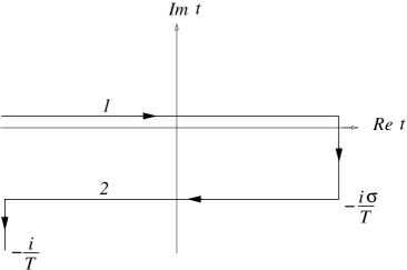
Figure 7: General time contour in the complex $t$-plane.

Here $\sigma$ is a constant and has the value in the range $0\leq\sigma\leq 1$. When $\sigma=0$ the description of the thermal field theory coincides with the closed time path formalism while for $\sigma=\frac{1}{2}$, the description corresponds to thermofield dynamics. In this section, we will show that a simple factorization of the thermal operator and, therefore, of a thermal graph takes place only for the cases when $\sigma=0,1$. In the case of closed time path corresponding $\sigma=0$, we have already seen this. Here we will study the behavior of the thermal propagator for a general time path in the complex $t$-plane.

Let us consider a theory describing a real scalar field. The doubling at finite temperature simply corresponds to introducing the fields $(\phi_{1},\phi_{2})$ on the two paths labelled $1,2$ (the original field that we start out with is considered to be $\phi_{1}$). For a general time contour as shown in Fig.4, it can be shown that

$$\Delta^{(T)}(p)=\left(\begin{array}[]{cc}\Delta_{11}^{(T)}(p)&\Delta_{12}^{(T)}(p)\\ \vskip 2.0pt\cr\Delta_{21}^{(T)}(p)&\Delta_{22}^{(T)}(p)\end{array}\right),$$ (101)

where

$$\Delta_{11}^{(T)}(p) = \Delta_{++}^{(T)}(p),$$

$$\Delta_{12}^{(T)}(p) = e^{\frac{\sigma p_{0}}{T}}\Delta_{+-}^{(T)}(p),$$

$$\Delta_{21}^{(T)}(p) = e^{-\frac{\sigma p_{0}}{T}}\Delta_{-+}^{(T)}(p),$$

$$\Delta_{22}^{(T)}(p) = \Delta_{--}^{(T)}(p),$$ (102)

where $\Delta_{ij}^{(T)}(p),i,j=\pm$ correspond to the propagators in the closed time path formalism that we have already discussed in the earlier section. Fourier transforming these components of the propagator in the energy variable, we obtain the mixed space propagator for the general contour to be

$$\Delta_{11}^{(T)}(t,E) = \Delta_{++}^{(T)}(t,E),$$

$$\Delta_{12}^{(T)}(t,E) = \Delta_{+-}^{(T)}(t+i\frac{\sigma}{T},E)=\frac{1}{\sinh\frac{E}{T}}\left[\sinh\left((1-\sigma)\frac{E}{T}\right)\ \Delta_{+-}^{(T)}(t,E)+\sinh\left(\frac{\sigma E}{T}\right)\ \Delta_{-+}^{(T)}(t,E)\right],$$

$$\Delta_{21}^{(T)}(t,E) = \Delta_{-+}^{(T)}(t-i\frac{\sigma}{T},E)=\frac{1}{\sinh\frac{E}{T}}\left[\sinh\left(\frac{\sigma E}{T}\right)\ \Delta_{+-}^{(T)}(t,E)+\sinh\left((1-\sigma)\frac{E}{T}\right)\ \Delta_{-+}^{(T)}(t,E)\right],$$

$$\Delta_{22}^{(T)}(t,E) = \Delta_{--}^{(T)}(t,E).$$ (103)

We note from (103) that in the limit $T\rightarrow 0$,

$$\Delta_{12}^{(T)}(t,E) \rightarrow e^{-\frac{\sigma E}{T}}\ \Delta_{+-}^{(T=0)}(t,E)+e^{(\sigma-1)\frac{E}{T}}\ \Delta_{-+}^{(T=0)}(t,E)$$

$$= \delta_{\sigma,0}\ \Delta_{+-}^{(T=0)}(t,E)+\delta_{\sigma,1}\ \Delta_{-+}^{(T=0)}(t,E),$$

$$\Delta_{21}^{(T)}(t,E) \rightarrow e^{(\sigma-1)\frac{E}{T}}\ \Delta_{+-}^{(T=0)}(t,E)+e^{-\frac{\sigma E}{T}}\ \Delta_{-+}^{(T=0)}(t,E)$$ (104)

$$= \delta_{\sigma,1}\ \Delta_{+-}^{(T=0)}(t,E)+\delta_{\sigma,0}\ \Delta_{-+}^{(T=0)}(t,E).$$

This shows that if $\sigma\neq 0,1$, the off-diagonal components of the propagator vanish (at $T=0$) leading to a decoupling of the two fields at zero temperature. When $\sigma=0,1$, the off-diagonal elements of the components do not vanish at zero temperature, nonetheless there is decoupling of the two degrees of freedom.

Since each component of the propagator in the closed time formalism has a simple factorization given by (89), it follows from (103) that for a general time contour we can write

$$\Delta^{(T)}(t,E)=\left(1+n(E)(1-S(E))L(\epsilon)\right)\tilde{\Delta}(t,E),$$ (105)

where

$$\tilde{\Delta}_{11}(t,E) = \Delta_{++}^{(T=0)}$$

$$\tilde{\Delta}_{12}(t,E) = \frac{1}{\sinh\frac{E}{T}}\left[\sinh\left((1-\sigma)\frac{E}{T}\right)\Delta_{+-}^{(T=0)}+\sinh\left(\frac{\sigma E}{T}\right)\Delta_{-+}^{(T=0)}\right]$$

$$\tilde{\Delta}_{21}(t,E) = \frac{1}{\sinh\frac{E}{T}}\left[\sinh\left(\frac{\sigma E}{T}\right)\Delta_{+-}^{(T=0)}+\sinh\left((1-\sigma)\frac{E}{T}\right)\Delta_{-+}^{(T=0)}\right]$$

$$\tilde{\Delta}_{22}(t,E) = \Delta_{--}^{(T=0)}.$$ (106)

It is clear from the above result that in the general case, temperature cannot be completely factored out of the matrix in a simple manner unless $\sigma=0,1$. For the case of thermofield dynamics where $\sigma=\frac{1}{2}$, it is easy to show that

$$\Delta^{(T)}(t,E)=\left(1+n(E)(1-S(E))L(\epsilon)\right)\left(\begin{array}[]{cc}1&e^{-\frac{E}{2T}}L(\epsilon)\\ e^{-\frac{E}{2T}}L(\epsilon)&1\end{array}\right)\Delta^{(T=0)}(t,E),$$ (107)

so that, in this case, the basic thermal operator takes a matrix form. As a result, the thermal operator representation for any graph in the formalism of a general contour (where $\sigma\neq 0,1$) is not so simple as in the imaginary time formalism or the closed time path formalism. However, it is worth noting that although in such cases there will be no simple factorization at the level of individual graphs, the simple factorization will occur for the complete set of graphs associated with a given physical amplitude (which follows from the fact that a physical amplitude is the same in any formalism).

V Summary

In this paper, we have systematically studied the interesting question of thermal operator representation for Feynman graphs at finite temperature. By working in a mixed space $(\tau,\vec{p}\ )$ (or $(t,\vec{p}\ )$), we have given a simpler derivation of the thermal operator representation in the imaginary time formalism. We have traced the origin of such a simple relation to the fact that the thermal propagator, in this space, has a basic factorization where the basic thermal operator is independent of time. We have also generalized the thermal operator representation to the case where there is a nontrivial chemical potential. In this case, although the thermal propagator also factorizes, the basic thermal operator involves a time derivative which leads to a thermal operator representation for any graph that is highly nontrivial. We have tried to study various properties of the thermal operator and have shown that it is a projection operator which projects functions into the space where the KMS periodicity condition is satisfied. We have also shown that there is a simple thermal operator representation in the closed time path formalism. The derivation, in this case, is even simpler than that for the imaginary time formalism. For a general time contour (including the one for thermofield dynamics), however, the thermal operator representation is not so simple as in the imaginary time formalism and the closed time path formalism.

Acknowledgment

This work was supported in part by the US DOE Grant number DE-FG 02-91ER40685, by MCT/CNPq as well as by FAPESP, Brazil and by CONICYT, Chile under grant Fondecyt 1030363 and 7040057 (Int. Coop.).

References

(1)
O. Espinosa and E. Stockmeyer, Phys. Rev. D69, 065004 (2004).
(2)
O. Espinosa, Phys. Rev. D71, 065009 (2005).
(3)
J.-P. Blaizot and U. Reinosa, hep-ph/0406109 (2004).
(4)
J. I. Kapusta, Finite Temperature Field Theory (Cambridge University
Press, Cambridge, England, 1989).
(5)
M. L. Bellac, Thermal Field Theory (Cambridge University Press,
Cambridge, England, 1996).
(6)
A. Das, Finite Temperature Field Theory (World Scientific, NY, 1997).
(7) E. Braaten and R. Pisarski, Nuc. Phys. B337,
569 (1990); Nuc. Phys. B339, 310 (1990).
(8) J. Frenkel and J. C. Taylor, Nuc. Phys. B334,
199 (1990), Nuc. Phys. B374, 156 (1992).
(9)
P. F. Bedaque and Ashok Das, Mod. Phys. Lett. A8, 3151 (1993).
(10)
A. K. Das and G. V. Dunne, Phys. Rev. D57, 5023 (1998).
(11)
J. S. Schwinger, J. Math. Phys. 2, 407 (1961).
(12)
P. M. Bakshi and K. T. Mahanthappa, J. Math. Phys. 4, 1
(1963);
L. V. Keldysh, Zh. Eksp. Teor. Fiz. 47, 1515 (1964).
(13) Y. Takahashi and H. Umezawa, Collective Phenomena
2, 55 (1975); H. Umezawa, H. Matsumoto and M. Tachiki, Thermofield Dynamics and Condensed States, North-Holland, Amsterdam
(1982).
(14)
R. Kubo, J. Phys. Soc. Japan 12, 570 (1957);
P. C. Martin and J. S. Schwinger, Phys. Rev. 115, 1342 (1959).